Nonlinear Excitations in Inflationary Power Spectra

Abstract

We develop methods to calculate the curvature power spectrum in models where features in the inflaton potential nonlinearly excite modes and generate high frequency features in the spectrum. The first nontrivial effect of excitations generating further excitations arises at third order in deviations from slow roll. If these further excitations are contemporaneous, the series can be resummed, showing the exponential sensitivity of the curvature spectrum to potential features. More generally, this exponential approximation provides a power spectrum template which nonlinearly obeys relations between excitation coefficients and whose parameters may be appropriately adjusted. For a large sharp step in the potential, it greatly improves the analytic power spectrum template and its dependence on potential parameters. For axionic oscillations in the potential, it corrects the mapping between the potential and the amplitude, phase and zero point of the curvature oscillations, which might otherwise cause erroneous inferences in for example the tensor-scalar ratio, formally even when that amplitude is $10^{3}$ times larger than the slow roll power spectrum. It also estimates when terms that produce double frequency oscillations that are usually omitted when analyzing data should be included. These techniques should allow future studies of high frequency features in the CMB and large scale structure to extend to higher amplitude and/or higher precision.

I Introduction

Features in the inflaton potential produce features in the curvature spectrum that are imprinted into cosmological observables of the cosmic microwave background (CMB) and large scale structure. In particular, the CMB power spectrum places strong, model-independent constraints on the amplitude of broad features that persist over more than an efold in wavenumber (e.g. Hannestad (2001); Hu and Okamoto (2004); Tegmark and Zaldarriaga (2002); Hannestad (2004); Bridle et al. (2003); Mukherjee and Wang (2003); Leach (2006); Peiris and Verde (2010); Hlozek et al. (2012); Gauthier and Bucher (2012); Vazquez et al. (2012); Hunt and Sarkar (2014); Aslanyan et al. (2014); Hazra et al. (2014); Ade et al. (2015)).

Sharp or high frequency features are more difficult to constrain both because they violate the ordinary slow roll approximation and their observable impact in the CMB is suppressed due to projection effects. Such features also have the ability to mimic local statistical fluctuations in data (e.g. Meerburg et al. (2014); Easther and Flauger (2014)) and so require accurate model predictions over a range of scales or observables to detect. This is often undertaken on a case by case basis, for example in axion monodromy Silverstein and Westphal (2008) and step potential models Adams et al. (2001). Indeed predictions for these two models have been extensively developed (e.g. Miranda and Hu (2014); Flauger et al. (2014) for improvements in range required for Planck CMB data) due to their ability to fit various anomalies in the CMB power spectrum Peiris et al. (2003); Flauger et al. (2010).

In this paper, we develop general techniques for predicting the curvature power spectrum for models with large, high frequency features. These features necessitate an extension of the ordinary slow roll approximation where not all slow roll parameters are considered to be slowly varying. Instead the prediction for the inflaton modefunction excitations can be iteratively improved using Green function techniques Stewart (2002a), typically up to at most second order in deviations from slow roll Choe et al. (2004a).

In Ref. Dvorkin and Hu (2010a) these techniques were further developed to predict percent level accurate CMB temperature power spectra for nearly order unity curvature fluctuations. By requiring conservation of superhorizon curvature fluctuations and positive definite power spectra, these techniques also provide a controlled approximation for the amplitude of even larger features but with diminished accuracy for their form. Analyses that utilized this technique imposed a prior on the amplitude of features that were not necessarily required by the data Dvorkin and Hu (2010b, 2011); Miranda et al. (2015). Furthermore the Planck data now require sub-percent level accuracy for small-scale features. Here we present techniques that go beyond second order perturbation theory to describe the fully nonlinear effect of potential features in the curvature power spectrum.

We begin in §II by developing the Green function approach directly for curvature excitations which unlike the inflaton excitations can be straightforwardly iterated to arbitrary order. The form of the resultant series is highly constrained by exact relations between the Bogoliubov excitation coefficients (e.g. Greene et al. (2004)). The first true nonlinearity of excitations generating further excitations occurs only beyond second order for high frequency features. For excitations generated at the same epoch, the series can be resummed to give the fully nonlinear effect of excitations. In §III we apply these model-independent techniques to the step and monodromy potentials and demonstrate that they give accurate predictions for larger than order unity features unlike those in the literature. We discuss these results in §IV.

II Iterating Curvature Excitations

We develop a systematic expansion of comoving curvature fluctuations generated by features in the inflaton potential in §II.1. We then relate this expansion to the excitation or Bogoliubov coefficients of curvature modefunctions to both isolate the superhorizon scale behavior of the curvature fluctuations and to exploit the nonlinear relationship between the positive and negative frequency components in §II.2. In §II.3, we express the observable curvature power spectrum in terms of these coefficients and compare it to second order perturbation theory for the inflaton modefunction. Finally in §II.4, we show that for high frequency features of arbitrary amplitude, the Bogoliubov relation constrains the form of power spectrum features and motivates a nonlinear resummation of the series expansion. This resummation is an exponentiation of the first order excitation that is exact if the excitations are all generated at the same epoch and more generally provides a physically motivated template whose parameters may be adjusted for better accuracy.

II.1 Curvature Modefunctions

For a canonical scalar inflaton $\phi$, comoving curvature fluctuations ${\cal R}$ obey the Mukhanov-Sasaki equation of motion

$$\left(\frac{d^{2}}{dx^{2}}-\frac{2}{x}\frac{d}{dx}+1\right){\cal R}=-\frac{2}{x}\frac{f^{\prime}}{f}\frac{d{\cal R}}{dx},$$ (1)

where $x=k\eta$ with $\eta=\int_{t}^{t_{\rm end}}dt/a(t)$ as the conformal time to the end of inflation, ${}^{\prime}=d/d\ln\eta$ and

$$f^{2}=4\pi^{2}\left(\frac{\dot{\phi}a\eta}{H}\right)^{2}=8\pi^{2}\frac{\epsilon_{H}}{H^{2}}(aH\eta)^{2}$$ (2)

as the source of curvature fluctuations. Here $\epsilon_{H}$ is the Hubble slow roll parameter. Curvature fluctuations are related to inflaton field fluctuations in spatially flat gauge as ${\cal R}=xy/f$, where $y$ satisfies

$$\frac{d^{2}y}{dx^{2}}+\left(1-\frac{2}{x^{2}}\right)y=\left(\frac{f^{\prime\prime}-3f^{\prime}}{f}\right)\frac{y}{x^{2}}.$$ (3)

While Eq. (1) and (3) are mathematically the same, solving this system in ${\cal R}$ vs. $y$ has both practical advantages and disadvantages. The advantage of using $y$ is that for a sufficiently large $x$, or equivalently long time before horizon crossing, the source on the right hand side (rhs) of Eq. (3) can be ignored. Solutions then correspond to de Sitter modefunctions and the choice of the Bunch-Davies vacuum picks out and normalizes the positive frequency solution

$$\lim_{x\rightarrow\infty}y(x)=y_{0}(x)\equiv(1+i/x)e^{ix}.$$ (4)

If variations in the source $f^{\prime}/f$ become comparable to or faster than the modefunction oscillation, i.e. $\Delta\ln\eta\lesssim 1/x$ for $x\gtrsim 1$, they cause non-adiabatic excitations of the modefunction out of the vacuum state. The same simplification of a universal initial form for the modefunction is not true for the curvature since ${\cal R}=xy/f$ depends explicitly on the source $f$.

For this reason, the original formulation of the generalized slow roll approach solved Eq. (3) for the field excitation in $y$ and related these solutions to the curvature fluctuations after horizon crossing Stewart (2002a); Choe et al. (2004b); Dvorkin and Hu (2010a). Starting from the universal $y_{0}$, the GSR approach replaces $y$ in the rhs source of Eq. (3) which then can be solved using Green function techniques. This procedure is then iterated to improve the solution to the desired order in $f^{\prime}/f$. The drawback of this approach is that if the source $f$ continues to vary outside the horizon then so will the inflaton modefunction since both the lhs and rhs of Eq. (3) scale as $y/x^{2}$. For potentials with high temporal frequency sources, this fact would lead to an apparent breakdown in perturbativity.

On the other hand, the curvature modefunction equation (1) has a superhorizon solution of ${\cal R}=$  const. for any source. Ref. Dvorkin and Hu (2010a) exploited this fact by including additional corrections from $f^{\prime}/f$ at each order in $y$ to keep ${\cal R}=xy/f$ constant for $x\ll 1$. This procedure is valid in perturbation theory since these terms already exist at the next order. However it is implemented by hand at each order and obscures the reason why the expansion should work when the inflation modefunction deviates substantially from the de Sitter $y_{0}$.

To eliminate this superhorizon problem and provide a technique where the iterative improvement is straightforwardly implemented, we establish here the equivalent GSR formalism for curvature modefunctions. This trades the superhorizon problem with an equivalent subhorizon problem that can more easily be finessed. As discussed above, on subhorizon scales the curvature depends explicitly on $f$, reflecting the fact that the comoving curvature fluctuation is not defined for a pure de Sitter background. To finesse this issue, let us exploit the fact that although $f$ can have short timescale transient evolution, it cannot have a large net evolution across many efolds without ending inflation. Thus let us assume that from some initial time $x=x_{0}$ through horizon crossing $x\ll 1$, $f$ is perturbatively close to some fiducial value $f_{*}$. At the end of the calculation, we cast the final results in a form that is independent of $f_{*}$ and send $x_{0}\rightarrow\infty$.

We can now iteratively improve the solution. Substituting ${\cal R}\rightarrow{\cal R}_{0}\equiv xy_{0}/f_{*}$ on the rhs of Eq. (1) yields the correction ${\cal R}_{1}$ and we can repeat this procedure to find ${\cal R}=\sum_{n=0}^{n_{\rm max}}{\cal R}_{n}$ to any desired order. From the Green function, the result is

$${\cal R}_{n}(x) = {\cal R}_{n}(x_{0})\frac{{\cal R}_{0}(x)}{{\cal R}_{0}(x_{0})}-i\int_{x}^{x_{0}}\frac{du}{u}\frac{f^{\prime}}{f}\frac{x}{u}\frac{d{\cal R}_{n-1}}{du}$$ (5)

$$\left[y_{0}^{*}(u)y_{0}(x)-y_{0}^{*}(x)y_{0}(u)\right],$$

where the initial value for the homogeneous solution is determined by the requirement that the inflaton modefunction is initially in the Bunch-Davies state,

$${\cal R}(x_{0}) = {\cal R}_{0}(x_{0})\frac{f_{*}}{f_{0}}={\cal R}_{0}(x_{0})\sum_{n=0}^{\infty}\frac{\ln^{n}(f_{*}/f_{0})}{n!}$$ (6)

$$\equiv \sum_{n=0}^{\infty}{\cal R}_{n}(x_{0}).$$

Here $f_{0}\equiv f(\ln x_{0})$ and while we could choose $f_{*}=f_{0}$ to eliminate these differences it is useful to keep these quantities distinct. For temporal sources with high frequency features, we can define $f_{*}$ as the mean over a few efolds rather than the instantaneous value of $f$ since the mean evolves slowly (see §II.4).

II.2 Bogoliubov Coefficients

It is useful to further characterize the positive and negative frequency components of the excitation through Bogoliubov coefficients

$${\cal R}_{n}(x)=\alpha_{n}(x){\cal R}_{0}(x)+\beta_{n}(x){\cal R}_{0}^{*}(x).$$ (7)

Inserting this form into Eq. (5), we obtain the Bogoliubov hierarchy equations

$$\alpha_{n}(x) = \frac{\ln^{n}(f_{*}/f_{0})}{n!}$$

$$+\int_{x}^{x_{0}}\frac{du}{u}\frac{f^{\prime}}{f}y_{0}^{*}[e^{iu}\alpha_{n-1}-e^{-iu}\beta_{n-1}],$$

$$\beta_{n}(x) = -\int_{x}^{x_{0}}\frac{du}{u}\frac{f^{\prime}}{f}y_{0}[e^{iu}\alpha_{n-1}-e^{-iu}\beta_{n-1}],$$ (8)

with $\alpha_{0}=1$, $\beta_{0}=0$. Note that we use the fact that

$$\frac{d{\cal R}_{n}(x)}{dx}=\alpha_{n}(x)\frac{d{\cal R}_{0}(x)}{dx}+\beta_{n}(x)\frac{d{\cal R}_{0}^{*}(x)}{dx}$$ (9)

by virtue of the Green function construction of Eq. (5). To evaluate this series to $n$th order, one simply performs $n$ one dimensional integrals sequentially as each excitation generates new excitations through their interaction with the source.

The two Bogoliubov coefficients $\alpha=\sum\alpha_{n}$, $\beta=\sum\beta_{n}$ are related for any excitation $f^{\prime}/f$. This can be seen more directly from the corresponding inflaton modefunction solutions $y(x)$ and $y^{*}(x)$. The Wronskian formed from the two solutions is constant by virtue of Eq. (3) and given by the $x\rightarrow\infty$ Bunch-Davies limit as

$$y\frac{dy^{*}}{dx}-y^{*}\frac{dy}{dx}=-2i.$$ (10)

Using $y=f{\cal R}/x$ and Eq. (9), we obtain

$$|\alpha(x)|^{2}=|\beta(x)|^{2}+\left(\frac{f_{*}}{f}\right)^{2},$$ (11)

which differs from the usual Bogoliubov relationship between inflaton modefunction coefficients if $f$ evolves away from $f_{*}$. This relationship will play a central role in defining the form of the power spectrum for subhorizon excitations below.

Finally in order to extract the superhorizon behavior of these excitations, it is useful to form a specific linear combination of the Bogoliubov coefficients. Note that

$$\lim_{x\rightarrow 0}\Re(y_{0}) = -\frac{x^{2}}{3},$$

$$\lim_{x\rightarrow 0}\Im(y_{0}) = \frac{1}{x}.$$ (12)

By defining $\alpha^{\pm}=(\alpha\pm\beta)/2$, we isolate the coefficients that multiply these terms. Eq. (8) implies that they obey

$$\alpha^{\pm}_{n}(x) = \frac{1}{2}\frac{\ln^{n}(f_{*}/f_{0})}{n!}+\int_{x}^{x_{0}}\frac{du}{u}\frac{f^{\prime}}{f}[y_{0}^{*}(u)\mp y_{0}(u)]$$ (13)

$$\times\left[\cos u\,\alpha^{-}_{n-1}+i\sin u\,\alpha^{+}_{n-1}\right].$$

By inspection, these coefficients then take the limiting forms

$$\lim_{x\rightarrow 0}\alpha^{+}_{n} = \frac{1}{x}{\cal O}\left(\frac{f^{\prime}}{f}\right)^{n},$$

$$\lim_{x\rightarrow 0}\alpha^{-}_{n} = {\cal O}\left(\frac{f^{\prime}}{f}\right)^{n}.$$ (14)

While $\alpha^{+}_{n}$ diverges outside the horizon, it multiplies the strongly convergent real part of $y_{0}$ and hence the superhorizon curvature,

$$\lim_{x\rightarrow 0}{\cal R}_{n}=\frac{2i}{f_{*}}\alpha^{-}_{n},$$ (15)

depends only on $\alpha^{-}(0)$. Likewise though both $\alpha$ and $\beta$ diverge as $1/x$ outside the horizon, their individual effects on the curvature cancel as is consistent with the Bogoliubov relation (11). A similar issue for the inflaton Bogoliubov coefficients is even more severe with divergences going as $1/x^{3}$ which cancel amongst terms Stewart (2002a); Dvorkin and Hu (2010a). This simple means of calculating the observable curvature fluctuations provides an advantage for the curvature coefficient approach over previous iterative approaches.

II.3 Curvature Power Spectrum

The curvature power spectrum simply follows from the superhorizon form of the curvature modefunction in Eq. (15)

$$\Delta^{2}_{\cal R}=\lim_{x\rightarrow 0}|{\cal R}(x)|^{2}=\frac{\left|2\alpha^{-}\right|^{2}}{f_{*}^{2}}=\frac{1}{f_{*}^{2}}\left|1+2\sum_{n=1}^{\infty}\alpha^{-}_{n}\right|^{2}.$$ (16)

For comparison to results from the inflaton modefunction expansion in the literature and their compatibility with the Bogoliubov relation (11), let us explicitly evaluate the power spectrum to second order

$$\ln\Delta_{\cal R}^{2} = -2\ln f_{*}+4\Re(\alpha^{-}_{1})$$

$$\quad+4[\Im^{2}(\alpha^{-}_{1})-\Re^{2}(\alpha^{-}_{1})+\Re(\alpha^{-}_{2})]+\ldots$$

The use of the log power spectrum facilitates comparisons to the literature and guarantees a positive definite power spectrum even if the excitations become nonperturbative.

From Eq. (13), the first line gives the zeroth and first order contributions as

$$\ln\Delta_{\cal R}^{2(1)} = -2\ln f_{*}+2(\ln f_{*}-\ln f_{0})$$ (18)

$$\quad+4\int_{x}^{x_{0}}\frac{du}{u}\frac{f^{\prime}}{f}\left(\cos^{2}u-\frac{\sin 2u}{2u}\right)$$

$$= -2\ln f_{0}+2\int_{x}^{x_{0}}\frac{du}{u}\frac{f^{\prime}}{f}\left[1-W_{f}(u)\right]$$

$$= -2\ln f-2\int_{x}^{x_{0}}\frac{du}{u}\frac{f^{\prime}}{f}W_{f}(u),$$

where

$$W_{f}(u)=\frac{\sin 2u}{u}-\cos 2u$$ (19)

with $W_{f}(0)=1$.

Thus the end result is independent of both the arbitrary fiducial normalization scale $f_{*}$ and the initial conditions $f_{0}$. We can therefore take $x_{0}\rightarrow\infty$ without loss of generality. The result also does not depend on the arbitrary superhorizon end point $x\ll 1$ as the integral simply represents the freezeout of $-2\ln f$ through the window $W_{f}$. For example, for a slowly varying $f=\bar{f}$, we can interpret this integral as representing a refinement of the leading order slow-roll freezeout condition $\Delta_{\cal R}^{2}=\bar{\Delta}_{\cal R}^{2}\approx 1/\bar{f}^{2}|_{x\approx 1}$. Note that

$$\int_{0}^{x_{0}}\frac{du}{u}\left[1-W_{f}(u)\right]\approx\ln x_{0}-\ln x_{f},$$ (20)

where $\ln x_{f}=2-\gamma_{E}-\ln 2\approx 0.7296$ and so for a constant $\ln\bar{f}^{\prime}$

$$\ln\bar{\Delta}_{\cal R}^{2(1)} \approx -2\ln\bar{f}_{0}-2(\ln\bar{f})^{\prime}(\ln x_{f}-\ln x_{0})$$ (21)

$$\approx -2\ln\bar{f}(\ln x_{f}).$$

Now let us compare the first order result as derived from inflaton modefunction iteration Stewart (2002a)

$$\ln\Delta_{\cal R}^{2}\approx G(\ln x)+\frac{2}{3}\int_{x}^{\infty}\frac{du}{u}W(u)\left(\frac{f^{\prime\prime}-3f^{\prime}}{f}\right),$$ (22)

where

$$G(\ln x) = -2\ln f+\frac{2}{3}(\ln f)^{\prime}.$$ (23)

and

$$W(u)={3\sin 2u\over 2u^{3}}-{3\cos 2u\over u^{2}}-{3\sin 2u\over 2u}.$$ (24)

Note that $W(0)=1$, $W(\infty)=0$ and

$$W_{f}(u)=W(u)+\frac{W^{\prime}(u)}{3}.$$ (25)

As noted in Ref. Dvorkin and Hu (2010a), this form is not well defined in that it depends on the arbitrary evaluation point $x\ll 1$ since the source in the integrand is not the derivative of the boundary term $G$. Even if $f^{\prime}/f$ = const. as in slow roll this would lead to an unphysical logarithmic evolution of the power spectrum outside the horizon. For a model with high frequency temporal features, the problem is much worse and can appear as a breakdown in the perturbation expansion near horizon crossing. Ref. Dvorkin and Hu (2010a) corrected this problem by replacing

$$\frac{2}{3}\left(\frac{f^{\prime\prime}-3f^{\prime}}{f}\right)\rightarrow G^{\prime}=-2(\ln f)^{\prime}+\frac{2}{3}(\ln f)^{\prime\prime},$$ (26)

which differ by a second order $(f^{\prime}/f)^{2}$ term. This brings the power spectrum to Stewart (2002a)

$$\ln\Delta_{\cal R}^{2({\rm GSR})}\approx G(\ln x)+\int_{x}^{\infty}\frac{du}{u}G^{\prime}(\ln u)W(u).$$ (27)

As we shall see this term does indeed appear in the second order expression, and so in perturbation theory, this procedure just amounts to regrouping existing terms. However this regrouping lacks an algorithmic formulation for a given term in the iterative series and obscures what the criteria is for breakdown of the perturbative expansion.

The curvature modefunction expansion provides a better derivation and justification for this procedure. Using Eq. (25) to integrate Eq. (18) by parts and assuming $x\ll 1$ and $x_{0}\gg 1$

$$\ln\Delta_{\cal R}^{2(1)} = -2\ln f+\frac{2}{3}(\ln f)^{\prime}$$ (28)

$$+\int_{x}^{x_{0}}\frac{du}{u}\left[-2(\ln f)^{\prime}+\frac{2}{3}(\ln f)^{\prime\prime}\right]W(u)$$

$$= G(\ln x)+\int_{x}^{x_{0}}\frac{du}{u}G^{\prime}(\ln u)W(u),$$

which agrees exactly with Eq. (27) once $x_{0}\rightarrow\infty$.

Thus the criteria for perturbative validity is that the curvature modefunction remains close to ${\cal R}\approx{\cal R}_{0}$, which is guaranteed outside the horizon if it is close at horizon crossing, as opposed to the inflaton modefunction $y\approx y_{0}$ for all time after horizon crossing. Our new curvature modefunction expansion is explicitly valid out to order unity curvature power spectrum features and can be straightforwardly iterated to arbitrary order.

Since the two forms in Eqs. (18) and (28) are mathematically identical, it is just a matter of convenience as to which representation to use. The $G^{\prime}$ form has some practical advantages since the kernel $W$ decays away inside the horizon whereas the analogous kernel for $(\ln f)^{\prime}$ oscillates out to infinity. Note that under the slow roll assumption of $f^{\prime}/f\approx$ const., $G=\bar{G}$ freezes out at a different epoch than $\bar{f}$ in determining the power spectrum

$$\bar{\Delta}_{\cal R}^{2(1)}\approx e^{\bar{G}(\ln x_{G})},$$ (29)

where $\ln x_{G}$ can be derived either directly or by matching the alternate form $e^{-2\ln\bar{f}(\ln x_{f})}$ so that $\ln x_{G}=\ln x_{f}+1/3$ (e.g. Motohashi and Hu (2015)).

We can likewise explicitly represent the second order terms in Eq. (II.3). The first new term is the square of a first order quantity

$$4\Im(\alpha^{-}_{1}) = 4\int_{x}^{x_{0}}\frac{du}{u}\frac{f^{\prime}}{f}\left(\cos u\sin u-\frac{\sin^{2}u}{u}\right)$$ (30)

$$= 2\int_{x}^{x_{0}}\frac{du}{u}\frac{f^{\prime}}{f}\left[-X(u)-\frac{1}{3}X^{\prime}(u)\right]$$

$$\approx \int_{x}^{\infty}\frac{du}{u}G^{\prime}(\ln u)X(u)\equiv\sqrt{2}I_{1}(x),$$

where

$$X(x)={3\over x^{3}}(\sin x-x\cos x)^{2},$$ (31)

with $X(0)=X(\infty)=0$. The intrinsically second order piece can be isolated as

$$4\Re(\alpha^{-}_{2})=4|\alpha^{-}_{1}|^{2}+I_{2},$$ (32)

where

$$I_{2}=-4\int_{x}^{x_{0}}\frac{du}{u}\frac{f^{\prime}}{f}\left[X(u)+\frac{1}{3}X^{\prime}(u)\right]\int_{u}^{x_{0}}\frac{dv}{v^{2}}\frac{f^{\prime}}{f}.$$ (33)

To second order we obtain

$$\ln\Delta_{\cal R}^{2(2)}=G(\ln x)+\int_{x}^{x_{0}}\frac{du}{u}G^{\prime}(\ln u)W(u)+I_{1}^{2}+I_{2},$$ (34)

which is exactly the same result as derived from the curvature conserving replacement procedure of Eq. (26) Dvorkin and Hu (2010a).

The nested integral in $I_{2}$ contains an extra $1/v$ that suppresses contributions from sources inside the horizon. In fact had we replaced $y_{0}\rightarrow e^{ix}$ in the evaluation of $\Re(\alpha^{-}_{2})$, the $I_{2}$ term would vanish identically, leaving the whole second order term a sum of squares of first order terms. For high frequency transient sources in $f^{\prime}/f$, these contributions are further suppressed by integrating to zero whereas modulation by $W(u)$ or $X(u)$ in the first order terms can generate large excitations out of transient sources as we discuss in the next section. Thus as noted in Ref. Dvorkin and Hu (2010a), for excitations that occur well inside the horizon it is generally a good approximation to neglect the intrinsically second order term $I_{2}$.

II.4 Subhorizon Excitations

For curvature excitations that are imprinted well before horizon crossing at $x\gg 1$, the general treatment of the previous sections simplifies considerably providing useful insights about the form of nonlinear excitations in the power spectrum.

In the Bogoliubov hierarchy equations (8), we can replace $y_{0}(x)\rightarrow e^{ix}$ in this $x\gg 1$ limit. The terms that couple $\alpha_{n}$ to $\alpha_{n-1}$ and $\beta_{n}$ to $\beta_{n-1}$ involve only the source $f^{\prime}/f$ whereas those that couple $\alpha_{n}$ to $\beta_{n-1}$ and $\beta_{n}$ to $\alpha_{n-1}$ modulate the source as $e^{\pm 2ix}f^{\prime}/f$. Let us first consider why the unmodulated pieces appear. Suppose we started the modes at $x_{0}$ with $\alpha_{0}=1$ and an impulsive excitation that provides a constant $\beta_{1}^{({\rm un})}=(f_{*}/f_{0})\beta_{1*}$ where we have scaled the constant $\beta_{1*}$ for reasons that will be clear below. With only the unmodulated terms in Eq. (8), these would evolve as

$$\alpha_{n}^{({\rm un})} = \frac{\ln^{n}(f_{*}/f_{0})}{n!}+\int_{x}^{x_{0}}\frac{du}{u}(\ln f)^{\prime}\alpha_{n-1}^{(\rm un)}=\frac{\ln^{n}(f_{*}/f)}{n!},$$

$$\beta_{n}^{({\rm un})} = \int_{x}^{x_{0}}\frac{du}{u}(\ln f)^{\prime}\beta_{n-1}^{(\rm un)}=\frac{\ln^{n-1}(f_{0}/f)}{(n-1)!}\frac{f_{*}}{f_{0}}\beta_{1*},$$ (35)

and hence resum to

$$\alpha^{({\rm un})} = \sum_{n=0}^{\infty}\alpha_{n}^{({\rm un})}=\frac{f_{*}}{f}\alpha_{0},$$

$$\beta^{({\rm un})} = \sum_{n=1}^{\infty}\beta_{n}^{({\rm un})}=\frac{f_{*}}{f}\beta_{1*}.$$ (36)

Thus we see that these terms in the hierarchy simply renormalize the Bogoliubov coefficients for the net evolution in $f$ in accordance with the Bogoliubov relation Eq. (11). This evolution does not represent a subsequent excitation generated by the original excitation. For example here $\alpha^{({\rm un})}=f_{*}/f$ still represents modes in the Bunch-Davies vacuum. Since the net change in $f$ is responsible for the slow-roll evolution of the curvature modefunctions, we will term this nonlinear rescaling “slow roll renormalization.”

The modulated terms in Eq. (8) represent excitations generating further excitations. For rapid variation in $f^{\prime}/f$, the slow roll renormalization terms can be small, leading to small overall deviations from scale invariance in the power spectrum while the modulated or excitation terms can be large and potentially nonlinear. While we cannot in general resum this series in closed form, we can still exploit the Bogoliubov relation (11) to constrain the form of their resummation. Removing the slow-roll renormalization, we can express the remaining piece in a manner that makes the Bogoliubov relation (11) manifest

$$|\alpha| = \frac{f_{*}}{f}\cosh\frac{B}{2},$$

$$|\beta| = \frac{f_{*}}{f}\sinh\frac{B}{2},$$ (37)

leaving an unspecified relative phase between them

$$\frac{\beta}{\alpha}=e^{i\varphi}\tanh\frac{B}{2}.$$ (38)

Now let us further assume that all of the excitations occur before horizon crossing so that apart from the slow roll renormalization, the source $f^{\prime}/f$ ceases to change $\alpha$ and $\beta$ or $\alpha^{\pm}$ at some $x\gg 1$. The power spectrum then takes the form

$$\Delta_{\cal R}^{2} = \frac{1}{f_{*}^{2}}(|\alpha|^{2}+|\beta|^{2}-2|\alpha||\beta|\cos\varphi)$$ (39)

$$= \frac{1}{f^{2}}(\cosh B-\sinh B\cos\varphi).$$

This form holds for an arbitrary amplitude excitation $B$ and guarantees a positive definite power spectrum since $\cosh B>\sinh B$. In fact it would continue to hold for excitations after horizon crossing, but as we have seen in §II.2, $|\beta|\rightarrow\infty$, and so $\alpha\rightarrow\beta$ and $\varphi\rightarrow 0$. Here the template form simply cancels to leading order.

Let us now see how this form arises in and illuminates the second order calculation. To second order, the Bogoliubov relation (11) gives

$$2\Re(\alpha_{1}) = 2(\ln f_{*}-\ln f),$$

$$2\Re(\alpha_{2}) = |\beta_{1}|^{2}-|\alpha_{1}|^{2}+2(\ln f_{*}-\ln f)^{2},$$ (40)

which makes the power spectrum

$$\Delta_{\cal R}^{2(2)} = \frac{1}{f_{*}^{2}}\Big{[}1+2\Re(\alpha_{1}+\alpha_{2}-\beta_{1}-\beta_{2}-\alpha_{1}\beta_{1}^{*})$$

$$\quad+|\alpha_{1}|^{2}+|\beta_{1}|^{2}\Big{]}$$

$$\approx \frac{1}{f_{*}^{2}}\left[\left(\frac{f_{*}}{f}\right)^{2}-2\Re(\beta_{1}+\beta_{2}+\alpha_{1}\beta_{1}^{*})+2|\beta_{1}|^{2}\right].$$

In the second line, we have exploited slow roll renormalization to replace the perturbative expansion of $f_{*}/f$ with its nonlinear resummation. The only term in the power spectrum that cannot be written in terms of first order quantities is $\Re(\beta_{2})$.

In the subhorizon excitation limit for $y_{0}$, the explicit forms for the coefficients simplify considerably. For the first order quantities,

$$\alpha_{1}(x) = \ln f_{*}-\ln f_{0}+\int_{x}^{x_{0}}\frac{du}{u}\frac{f^{\prime}}{f}$$

$$= \ln f_{*}-\ln f,$$

$$\beta_{1}(x) = -\int_{x}^{x_{0}}\frac{du}{u}\frac{f^{\prime}}{f}e^{2iu}.$$ (42)

Note that $\alpha_{1}$ is consistent with the Bogoliubov relation for $\Re(\alpha_{1})$ in Eq. (40) and is itself a real quantity. It appears as the first term in the slow roll renormalization of $\alpha_{0}=1$ to $\alpha=f_{*}/f$.

Using these quantities in Eq. (8) to define the second order quantities gives

$$\alpha_{2}(x) = \frac{(\ln f_{*}-\ln f)^{2}}{2}+\int_{x}^{x_{0}}\frac{du}{u}\frac{f^{\prime}}{f}e^{-2iu}\int_{u}^{x_{0}}\frac{dv}{v}\frac{f^{\prime}}{f}e^{2iv},$$

$$\beta_{2}(x) = (\ln f_{*}-\ln f_{0})\beta_{1}-\int_{x}^{x_{0}}\frac{du}{u}\frac{f^{\prime}}{f}e^{2iu}\int_{u}^{x_{0}}\frac{dv}{v}\frac{f^{\prime}}{f}$$ (43)

$$\quad-\int_{x}^{x_{0}}\frac{du}{u}\frac{f^{\prime}}{f}\int_{u}^{x_{0}}\frac{dv}{v}\frac{f^{\prime}}{f}e^{2iv}$$

$$= \alpha_{1}\beta_{1}.$$

Since

$$2\Re\left[\int_{x}^{{x_{0}}}duF(u)\int_{u}^{{x_{0}}}{dv}F^{*}(v)\right]=\left|\int_{x}^{{x_{0}}}duF(u)\right|^{2},$$ (44)

we recover Eq. (40) for $\Re(\alpha_{2})$ and in the subhorizon excitation limit $\Re(\beta_{2})$ can also be written in terms of first order quantities. This is of course just a restating of the fact that the $I_{2}$ contribution in Eq. (33) is negligible and comes from the deviation of $y_{0}(u)$ from $e^{iu}$. In fact $\alpha_{1}$ appears here because it is the first term in the slow roll renormalization of $\beta_{1}$, $\beta_{1}+\alpha_{1}\beta_{1}\approx(f_{*}/f)\beta_{1}$ and each further order will contain terms that resum to the full correction as shown in Eq. (36).

We can combine these terms back into the template form of Eq. (39),

$$\Delta_{\cal R}^{2(2)} \approx \frac{1}{f_{*}^{2}}\left[\left(\frac{f_{*}}{f}\right)^{2}+2|\beta_{1}|^{2}-2\left(\frac{f_{*}}{f}\right)^{2}\Re(\beta_{1})\right]$$ (45)

$$\approx \frac{1}{f^{2}}[\cosh(2|\beta_{1}|)-\sinh(2|\beta_{1}|)\cos\varphi],$$

where we have inserted the appropriate cubic and higher order terms that appear due to slow roll renormalization to factor out $(f_{*}/f)^{2}$. We can now associate $B=2|\beta_{1}|$ and $\varphi$ with the absolute phase of $\beta_{1}=e^{i\varphi}B/2$. Phrased in this form, the first order calculation of the power spectrum is in fact accurate to second order.

Eq. (45) automatically accounts for the resummed, slow roll renormalization of $f$ due to its evolution from the excitation epoch to horizon crossing. To make the correspondence between the nonlinearly resummed renormalization and the first order excitation general and explicit, let us model

$$\ln f=\ln\bar{f}+\delta\ln f,$$ (46)

where we take a log-linear evolution

$$\ln\bar{f} = \ln f_{*}+\frac{n_{s}-1}{2}[\ln(k_{0}\eta)-\ln x_{f}]$$ (47)

$$= \ln f_{*}+\frac{n_{s}-1}{2}[\ln x-\ln(k/k_{0})-\ln x_{f}].$$

Here the slope, or as we shall see the power spectrum tilt, $n_{s}=$  const., $k_{0}\eta=x_{f}$ defines the zero point, and the freezeout point $x=x_{f}$ is given by Eq. (20). Through Eq. (21), the model for $\ln\bar{f}$ defines a power spectrum that is a power law to leading order

$$\bar{I}_{0} \equiv \ln\bar{\Delta}_{\cal R}^{2}=-2\ln f_{*}+(n_{s}-1)\ln(k/k_{0}),$$ (48)

which can be used to replace the slow roll term in Eq. (45) $1/f^{2}\rightarrow e^{\bar{I}_{0}}$. For notational convenience let us define

$$\delta I_{0} = \ln\Delta_{\cal R}^{2(1)}-\ln\bar{\Delta}_{\cal R}^{2}$$

$$= -2\delta\ln f_{0}+4\int_{x}^{x_{0}}\frac{du}{u}(\delta\ln f)^{\prime}\left(\cos^{2}u-\frac{\sin 2u}{2u}\right),$$

and similarly

$$\delta I_{1} = I_{1}-\bar{I}_{1}$$

$$= 2\sqrt{2}\int_{x}^{x_{0}}\frac{du}{u}(\delta\ln f)^{\prime}\left(\cos u\sin u-\frac{\sin^{2}u}{u}\right),$$

where

$$\bar{I}_{1}=\frac{\pi}{2\sqrt{2}}(1-n_{s}).$$ (51)

Comparing with Eq. (42) at $u\gg 1$, we see that $\delta I_{0}$ and $\delta I_{1}$ capture the subhorizon excitation as

$$4\alpha^{-}_{1}=2(\alpha_{1}-\beta_{1})\rightarrow\delta I_{0}+i\sqrt{2}\delta I_{1},$$ (52)

whereas $\bar{I}_{0}$ captures the slow-roll renormalization of $\alpha_{1}$ and $\beta_{1}$ from the excitation. The second order power spectrum for subhorizon excitations then becomes

$$\Delta_{\cal R}^{2(2)}=\bar{\Delta}_{\cal R}^{2}\left[\bar{I}_{1}^{2}+\bar{I}_{2}+\cosh B-\sinh B\cos\varphi\right],$$ (53)

where $\bar{I}_{2}=-(n_{s}-1)^{2}$ and

$$B^{2} \approx \delta I_{0}^{2}+2\delta I_{1}^{2},$$

$$\cos\varphi \approx -\frac{\delta I_{0}\cos\bar{\varphi}-\sqrt{2}\delta I_{1}\sin\bar{\varphi}}{\sqrt{\delta I_{0}^{2}+2\delta I_{1}^{2}}}$$ (54)

$$\equiv \cos(\bar{\varphi}+\delta\varphi),$$

with

$$\bar{\varphi}=-\sqrt{2}\bar{I}_{1}=-\frac{\pi}{2}(1-n_{s}).$$ (55)

We include $\bar{I}_{1}$ as a phase shift $\bar{\varphi}$ since it can alternately be derived by keeping track of the phase difference between the positive and negative frequency components using Hankel functions for slow-roll modefunctions in the presence of tilt. This ensures that its effect is well modeled even for high amplitude excitations where the second order approximation has broken down. Finally in Eq. (53), the correction terms to the leading order slow roll power spectrum nearly cancel

$$\bar{I}_{1}^{2}+\bar{I}_{2}=\left(\frac{\pi^{2}}{8}-1\right)(1-n_{s})^{2},$$ (56)

and for viable $1-n_{s}\approx 0.03$ produce $\sim 10^{-4}$ corrections which we can typically neglect.

To summarize the subhorizon second order results, nonlinear effects from excitations generating excitations only appear through $\delta I_{2}$ which is negligible for subhorizon high-frequency excitations. This is a consequence of the Bogoliubov relation (11) for $\Re(\alpha_{2})$ and the fact that $\beta_{2}$ is simply a rescaling of the linear excitation $\beta_{1}$.

Thus the first true effect of subhorizon excitations generating further excitations occurs at third order. Even for subhorizon effects, third order excitations do not reduce exactly to products of first order excitations. In particular since

$$\beta_{3}(x) \approx -\int_{x}^{x_{0}}\frac{du}{u}\frac{f^{\prime}}{f}[e^{2iu}\alpha_{2}-\beta_{2}],$$ (57)

the cubic excitation involves $\Im(\alpha_{2})$, which is not determined by the Bogoliubov relation. On the other hand, these higher order coefficients are repeated integrations of the same fundamental modulated source of excitation $e^{2iu}f^{\prime}/f$ that is responsible for $\beta_{1}$. As shown in Eq. (36), the unmodulated $f^{\prime}/f$ pieces are responsible for slow roll renormalization. Thus the modulated or excitation part of the hierarchy is a function of the first order excitation function $\beta_{1}(u)$

$$\alpha_{n}(x) \approx -\int_{x}^{x_{0}}\frac{du}{u}\beta_{1}^{\prime*}(u)\beta_{n-1}(u),$$

$$\beta_{n}(x) \approx -\int_{x}^{x_{0}}\frac{du}{u}\beta_{1}^{\prime}(u)\alpha_{n-1}(u).$$ (58)

If we take $\beta_{1}=e^{i\varphi}|\beta_{1}|$ and further assume $\varphi\approx$ const. as would be the case if all excitations were generated at one epoch,

$$\alpha_{n}(x) \approx \begin{cases}|\beta_{1}|^{n}/n!&\quad(n={\rm even}),\\ 0&\quad(n={\rm odd}),\\ \end{cases}$$

$$\beta_{n}(x) \approx \begin{cases}0&\quad(n={\rm even}),\\ e^{i\varphi}|\beta_{1}|^{n}/n!&\quad(n={\rm odd}),\\ \end{cases}$$ (59)

which resums into

$$\alpha \approx \cosh|\beta_{1}|,$$

$$\beta \approx e^{i\varphi}\sinh|\beta_{1}|.$$ (60)

Thus we expect excitations to generate further excitations leading to an exponentiation of the linearized effect on the power spectrum. In this constant phase approximation, Eq. (54) for $B$ and $\varphi$ associated with the linear calculation are the fully nonlinear relation for the template power spectrum

$$\Delta^{2({\rm NL})}_{{\cal R}}\approx\bar{\Delta}_{\cal R}^{2}(\cosh B-\sinh B\cos\varphi).$$ (61)

Beyond cases where the constant phase approximation holds, we call the combination of Eqs. (54) and (61) the nonlinear (NL) ansatz. Errors induced by this prescription take the form of changes to $B(k)$ and $\varphi(k)$ rather than extra terms that make the power spectrum unphysical in single field inflation.

This ansatz should be compared with a similar exponentiation of $\delta I_{0}$ proposed in Ref. Dvorkin and Hu (2010a)

$$\Delta^{2({\rm GSR1})}_{{\cal R}} \equiv e^{I_{0}}(1+I_{1}^{2})$$ (62)

$$= \bar{\Delta}_{\cal R}^{2}e^{\delta I_{0}}[1+(\bar{I}_{1}+\delta I_{1})^{2}],$$

which equally well satisfies the second order form Eq. (34) for subhorizon excitations and preserves a positive definite power spectrum but differs in not explicitly enforcing the Bogoliubov relation (11). It is therefore limited in accuracy to order unity excitations $\sqrt{2}|\delta I_{1}|<1$ Dvorkin and Hu (2010b) whereas Eq. (61) is not. We shall next compare the NL ansatz to the exact result for explicit examples of potential features.

III Featured Examples

We apply the formalism developed in the previous section to two examples of high frequency features: sharp steps (§III.1) and axion monodromy oscillations (§III.2) in the inflaton potential. In the sharp step limit, all excitations are generated at the same epoch and the nonlinear resummation of the excitation hierarchy in the template form of Eq. (61) is exact for subhorizon modes. Deviations due to the finite duration of the excitation can be characterized by small changes in the parameters of the template form. For monodromy, in addition to excitations contemporaneously generating excitations that can be resummed, excitations resonantly generate excitations over an extended period of time. These too may be computed from cubic and higher order terms in the hierarchy and mainly produce changes in the parameters of the template form.

III.1 Sharp Steps

A sharp step in the potential provides a simple example where the excitation hierarchy ($\alpha_{n}$, $\beta_{n}$) of Eq. (8) and hence Eq. (61) can be explicitly calculated in closed form. We model the step potential as

$$V(\phi)=\bar{V}(\phi)\{1+2b_{V}[S(\phi-\phi_{s})-1]\},$$ (63)

where $-\infty<b_{V}<1/2$ and $S$ is a step function defined to be 0 before the step at $\phi_{s}$ and 1 after the step. Note that $b_{V}>0$ therefore is a step up, which is bounded by stepping from zero, and $b_{V}<0$ a step down to a fixed $\bar{V}(\phi)$, which is unbounded. Here $\bar{V}(\phi)$ is an underlying smooth slow-roll potential. In numerical comparisons, we take $\bar{V}(\phi)=V_{0}(1-\beta\phi^{2}/6)$ for definiteness.

III.1.1 Nonlinear Excitations

In order to evaluate the excitation hierarchy, we need a model for $(\delta\ln f)^{\prime}$. Since $f^{2}\propto\epsilon_{H}\propto\dot{\phi}^{2}$ with the time evolution of other terms subdominant, this amounts to understanding the change in the kinetic energy of the inflaton due to rolling over a step. Following Ref. Miranda and Hu (2014), we can start by using energy conservation to model the jump across the step

$$\Delta\ln f \equiv \frac{1}{2}\Delta\ln\epsilon_{H}=\frac{1}{2}(\ln\epsilon_{HI}-\ln\epsilon_{HB})$$ (64)

$$= \frac{1}{2}\ln\left(1-6b_{V}/\epsilon_{HB}\right),$$

where $\epsilon_{H}=\epsilon_{HB}$ before the step and $\epsilon_{HI}$ immediately after the step. Given that the step is sharp

$$(\delta\ln f)^{\prime}=(\Delta\ln f)S^{\prime},$$ (65)

where note that ${}^{\prime}=d/d\ln\eta\approx-d/dN$. Integrating to larger values in $\ln x$ goes from after the step to before the step which changes $S$ by $-1$. Thus $S^{\prime}$ is the negative of a delta function

$$\int_{x}^{\infty}\frac{du}{u}S^{\prime}=-S(x).$$ (66)

Using this model we can evaluate the $\alpha$ and $\beta$ hierarchy of coefficients for a sharp step. We assume that the modes in question encounter the step deep within the horizon $x_{s}=k\eta(N_{s})\gg 1$ and that the width of the step $\delta x_{s}=k\delta\eta(N_{s})\ll 1$. We will return to violations of these assumptions at low and high $k$ below. Starting with $\alpha_{0}=1$, $\beta_{0}=0$, we can evaluate the first order excitations with Eq. (8),

$$\alpha_{1} = (-\Delta\ln f)S,$$

$$\beta_{1} = -e^{2ix_{s}}(-\Delta\ln f)S.$$ (67)

Since each successive term adds a factor of $S$ which is then multiplied by $S^{\prime}$ from the source $(\ln f)^{\prime}$, the integrals reduce to evaluating

$$\int_{x}^{\infty}\frac{du}{u}S^{n-1}S^{\prime}=\frac{1}{n}\int_{x}^{\infty}\frac{du}{u}\frac{dS^{n}}{d\ln u}=-\frac{1}{n}S^{n}(x).$$ (68)

Thus the hierarchy of Bogoliubov coefficients is given explicitly by

$$\alpha_{n} = \frac{2^{n-1}}{n!}(-\Delta\ln fS)^{n},$$

$$\beta_{n} = -\frac{2^{n-1}}{n!}(-\Delta\ln fS)^{n}e^{2ix_{s}}.$$ (69)

Summing the series, we have immediately after the step

$$\alpha_{I} \equiv \sum_{n}\alpha_{n}=\frac{1}{2}+\frac{1}{2}e^{-2\Delta\ln f},$$

$$\beta_{I} \equiv \sum_{n}\beta_{n}=\left(\frac{1}{2}-\frac{1}{2}e^{-2\Delta\ln f}\right)e^{2ix_{s}}.$$ (70)

Note that this resummation satisfies the Bogoliubov relation (11)

$$|\alpha_{I}|^{2}-|\beta_{I}|^{2}=e^{-2\Delta\ln f}=\left(\frac{f_{B}}{f_{I}}\right)^{2}.$$ (71)

Now we need to evolve the coefficients from the step through to freezeout. The kinetic energy imparted by the step decays back to the attractor value after several efolds. On the attractor $\bar{\phi}_{,N}\approx-V_{,\phi}/3H^{2}$ and so the excess $\delta\phi_{,N}=\phi_{,N}-\bar{\phi}_{,N}$ evolves under the Klein-Gordon equation as

$$\delta\phi_{,NN}=-3\delta\phi_{,N}.$$ (72)

Thus this excess decays with efolds as

$$\delta\phi_{,N}\propto e^{-3(N-N_{s})}$$ (73)

where $N_{s}$ is the efold at which the inflaton encounters a step. This generalizes the treatment of Ref. Miranda and Hu (2014) to extremely large amplitude steps.

Since $\epsilon_{H}=(\phi_{,N})^{2}/2$, after many efolds $f\rightarrow f_{A}=f_{B}$. Since this evolution is slow compared with $\Delta x=1$, it simply renormalizes the coefficients as discussed in §II.4

$$\alpha_{A} = \frac{f_{I}}{f_{A}}\alpha_{I}=e^{\Delta\ln f}\alpha_{I}=\cosh(\Delta\ln f),$$

$$\beta_{A} = \frac{f_{I}}{f_{A}}\beta_{I}=e^{\Delta\ln f}\beta_{I}=\sinh(\Delta\ln f)e^{2ix_{s}},$$ (74)

which again satisfies the Bogoliubov relation

$$|\alpha_{A}|^{2}-|\beta_{A}|^{2} = \cosh^{2}(\Delta\ln f)-\sinh^{2}(\Delta\ln f)$$ (75)

$$= 1=\left(\frac{f_{B}}{f_{A}}\right)^{2}.$$

From Eqs. (37) and (38), we can read off the nonlinear template amplitude and phase

$$B = 2\Delta\ln f=\ln\left(1-6b_{V}/\epsilon_{HB}\right),$$

$$\delta\varphi = 2x_{s}.$$ (76)

There is no restriction on the amplitude of the step $b_{V}$, save that if $6b_{V}>\epsilon_{HB}$ the initial kinetic energy is insufficient to carry the inflaton over the step up.

This description suffices for modes that were deep inside the horizon when the inflaton rolled over the step but not so deep that the mode oscillates during the transition. Using the first-order-based template prescription for $B$ of Eq. (54) we can extend the description into these regimes. As in Eq. (52), we replace $2(\alpha_{1}-\beta_{1})$ with

$$\delta I_{0} = \frac{2\Delta\ln f}{3}{\cal D}\left(\frac{x_{s}}{x_{d}}\right)W^{\prime}(x_{s}),$$

$$\sqrt{2}\delta I_{1} = \frac{2\Delta\ln f}{3}{\cal D}\left(\frac{x_{s}}{x_{d}}\right)X^{\prime}(x_{s}).$$ (77)

Following Ref. Adshead et al. (2012); Miranda and Hu (2014) we account for a finite width step with a damping function ${\cal D}$, which for a step shape

$$S=\frac{1}{2}\left[\tanh\left(\frac{\phi-\phi_{s}}{d}\right)+1\right]$$ (78)

is given by

$${\cal D}(y)=\frac{y}{\sinh y}.$$ (79)

Here the damping scale

$$x_{d}=\frac{\phi^{\prime}}{\pi d},$$ (80)

and we have assumed for definiteness that the inflaton rolls over the step at $\phi_{s}$ toward larger field values. Thus the amplitude parameter becomes

$$B = \sqrt{\delta I_{0}^{2}+2\delta I_{1}^{2}}$$

$$= \ln\left(1-\frac{6b_{V}}{\epsilon_{HB}}\right){\cal D}\left(\frac{x}{x_{d}}\right)\frac{\sqrt{{W^{\prime}}^{2}(x_{s})+{X^{\prime}}^{2}(x_{s})}}{3}$$

and the phase

$$\cos\varphi=-\frac{W^{\prime}(x_{s})\cos\bar{\varphi}-X^{\prime}(x_{s})\sin\bar{\varphi}}{\sqrt{{W^{\prime}}^{2}(x_{s})+{X^{\prime}}^{2}(x_{s})}}.$$ (82)

This prescription exactly coincides with that given in Ref. Miranda and Hu (2014) to second order in the perturbation to the kinetic energy $6b_{V}/\epsilon_{HB}$ and generalizes it to arbitrarily large steps by matching it to the fully nonlinear calculation in the regime $1\ll x_{s}\ll x_{d}$.

Figure 1: First order curvature response $\delta I_{0}$ to an extremely large, sharp step: $6b_{V}/\epsilon_{HB}=-5.34$, $x_{d}\approx 750$ at $\eta_{s}=3299.780$ Mpc. Compared are the numerical result of integrating the source $f^{\prime}/f$ (exact, solid), the analytic second order approximation from Ref. Miranda and Hu (2014) (MH14, dotted) and the nonlinear analytic approximation of this work (NL, dashed) with differences with exact highlighted (bottom panel). In the region between the start of the oscillations and their damping, the NL provides a highly accurate form whereas MH14 is discrepant at order unity.

III.1.2 Comparisons and Fits

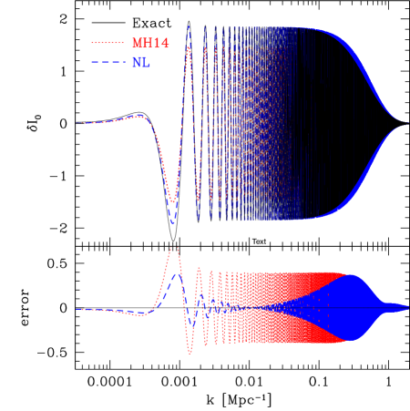
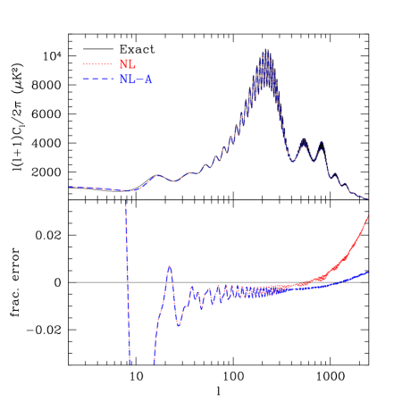
In Fig. 1 we show an example with a very large step $6b_{V}/\epsilon_{HB}=-5.34$ which the inflaton crosses when the horizon is comparable to the current horizon $\eta_{s}=3299.780$ Mpc. We first compare $\delta I_{0}$ as calculated exactly from $f(\ln\eta)$, our nonlinear calculation of Eq. (77) and the second order calculation of Ref. Miranda and Hu (2014). Although $\delta I_{0}$ is the first order response of the curvature modefunctions to the source, the source itself is nonlinear in the sense of imparting a large change in the kinetic energy of the inflaton. In the region $1\ll x_{s}\ll x_{d}$, our nonlinear (NL) analytic calculation accurately models the amplitude of the oscillations whereas that of Ref. Miranda and Hu (2014) (MH14) does not. Here $x_{d}\approx 750$ and $x_{s}=1$ at $k\approx 0.0003$ Mpc^-1. We follow the prescription in Ref. Miranda and Hu (2014) for relating these parameters to those of the potential.

Figure 2: Curvature power spectrum $\Delta_{\cal R}^{2}$ for the extremely large step of Fig. 1 (left, $6b_{V}/\epsilon_{HB}=-5.34$, $\eta_{s}=3299.78$ Mpc) and a large step (right, $6b_{V}/\epsilon_{HB}=0.2$, $\eta_{s}=3299.79$ Mpc) each with $x_{d}\approx 750$. Compared are the numerical result (exact, solid), the GSR1 second order form of Eq. (28) and the nonlinear form of Eq. (61). Both analytic forms use the same nonlinear analytic calculation of $\delta I_{0}$ and $\delta I_{1}$ from Fig. 1. Even at extremely large amplitudes the NL form provides a highly accurate description whereas GSR1 using the same first order responses does not. At amplitudes below unity, both perform well but NL generally exceeds the accuracy of GSR1.

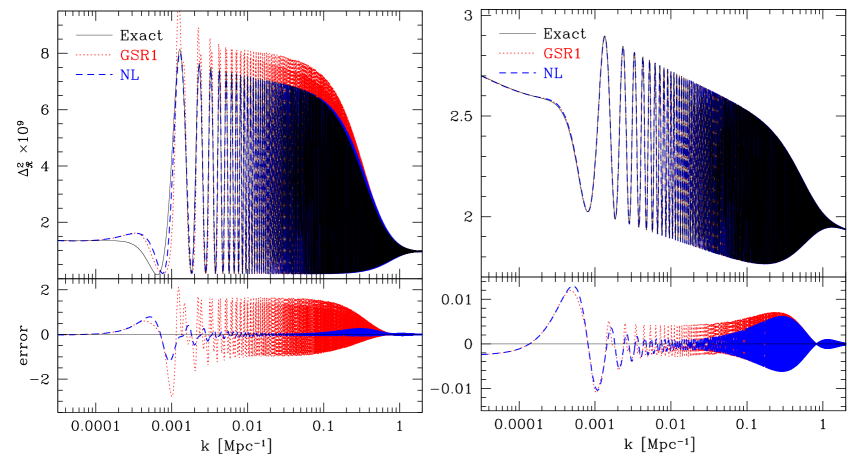
Even with the correct nonlinear $\delta I_{0}$, the GSR1 second order based form of Eq. (28) errs in predicting the power spectrum. In Fig. 2, we compare the exact power spectrum to the GSR1 form and our new nonlinear form. The NL again agrees well with the exact form for $1\ll x_{s}\ll x_{d}$ whereas even with the better analytic calculation of $\delta I_{0}$ from Fig. 1, GSR1 does not. We also show a smaller step ($6b_{V}/\epsilon_{HB}=0.2$) where the second order GSR1 approximation should be valid. In this case both GSR1 and NL perform well but NL is still markedly better in the region $1\ll x_{s}\ll x_{d}$.

Figure 3: CMB temperature power spectrum $C_{\ell}$ for the extremely large step and moderately large step cases of Fig. 2. Errors in $C_{\ell}$ are even smaller than in $\Delta_{\cal R}^{2}$ due to projection effects.

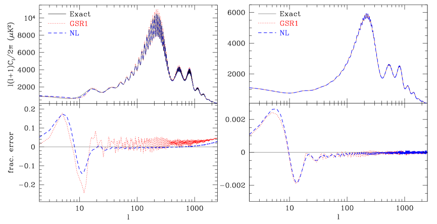
The errors in the CMB power spectrum are even smaller due to projection effects as shown in Fig. 3. Because projection effects also fill in the power at the oscillation troughs, here we plot fractional errors for an easier comparison with cosmic variance limits. Even for the large amplitude step the errors for $x\ll x_{d}$ are comparable to or smaller than cosmic variance errors through the damping tail. For the smaller amplitude step, both are.

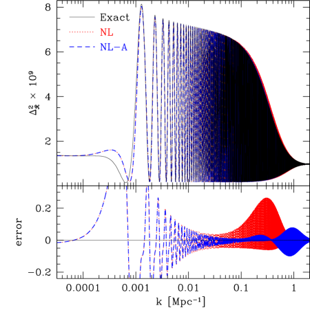
In fact most of the error in NL is not an error in the form of the template but rather a slight misassociation of the location $\eta_{s}$ and damping scale $x_{s}$ of the step given potential parameters. In Fig. 4 we show the result of adjusting these parameters. The main improvement is in the scale at which damping sets in due to a $\sim 7\%$ decrease in $x_{d}$. The small adjustment in $\eta_{s}$ makes the phase a better match for $x<x_{d}$ with only a $3\times 10^{-5}$ change. For the analysis of the observational data, these small corrections can be applied after the constraints on $6b_{V}/\epsilon_{HB}$, $\eta_{s}$ and $x_{d}$ are obtained with the NL template.

Because damping makes a change in how efficiently excitations generate further excitations we expect a change in the phase at $x>x_{d}$ that is not captured by the NL form. Since its effect comes in after the oscillations have already damped, this is a small problem even for extremely large step. If desired it can be fixed by introducing a running to the phase offset $\bar{\varphi}(\ln k)$ in Eq. (54).

Figure 4: Curvature and CMB temperature power spectrum for the extremely large step case of Fig. 2. The error in the damping of the oscillations can be further reduced from the NL model (dotted) by adjusting the location and width of the feature to $\eta_{s}\rightarrow 1.000029\eta_{s}$ and $x_{d}\rightarrow 0.936x_{d}$ with the same form (NL-A, dashed). Remaining errors are comparable to or less than cosmic variance out to the CMB damping scale even for this extremely large amplitude.

III.2 Monodromy

Our second example is axion monodromy where the potential is given by Silverstein and Westphal (2008)

$$V(\phi)=\bar{V}(\phi)+\Lambda^{4}\cos\left(\frac{\phi}{f_{a}}+\theta\right).$$ (83)

We assume that $\Lambda^{4}/\bar{V}\ll\bar{\epsilon}_{H}$ so that the inflaton can roll down the potential through the oscillations and that $f_{a}\ll 1$ in Planck units. Here again $\bar{V}(\phi)$ is an underlying smooth slow-roll potential which in examples we take as $\bar{V}=\lambda\phi$ so that $\bar{\epsilon}_{H}\approx 1/2\phi^{2}$.

III.2.1 Source Model

In order to calculate the excitations due to the oscillatory piece, we again need a model for the $f^{\prime}/f$. Following Refs. Dvorkin and Hu (2010a); Motohashi and Hu (2015) we can in general approximate

$$G^{\prime}+\frac{2}{3}\left(\frac{f^{\prime}}{f}\right)^{2}\approx 3\left(\frac{V_{,\phi}}{V}\right)^{2}-2\left(\frac{V_{,\phi\phi}}{V}\right),$$ (84)

up to $\epsilon_{H}$ suppressed corrections. Since $f_{a}\ll 1$, the $V_{,\phi\phi}$ term from the oscillations is dominant over the slow roll contributions $G^{\prime}\approx\delta G^{\prime}$. The $V_{,\phi}$ term is suppressed compared with the second by ${\cal O}(\sqrt{\bar{\epsilon}_{H}}f_{a})$ which we neglect. Since the oscillatory part of the potential makes only transient changes to the rolling of the inflaton we take Flauger et al. (2010)

$$\phi\approx\phi_{*}+\sqrt{2\bar{\epsilon}_{H}}\ln(x/x_{*}),$$ (85)

where $x_{*}$ is a suitably chosen normalization epoch which we optimize below (see Motohashi and Hu (2015)). For sufficiently small $\Lambda^{4}/\bar{V}$ we can drop the quadratic term $(f^{\prime}/f)^{2}$ in Eq. (84) and integrate

$$\delta G^{\prime}=-2(\delta\ln f)^{\prime}+\frac{2}{3}(\delta\ln f)^{\prime\prime}$$ (86)

to define the oscillatory excitation source

$$\delta\ln f=-3\frac{\Lambda^{4}}{\bar{V}}\frac{\omega\cos(\omega\ln x+\psi)+3\sin(\omega\ln x+\psi)}{f_{a}^{2}\omega(\omega^{2}+9)},$$ (87)

where the log frequency $\omega=\sqrt{2\bar{\epsilon}_{H}}/f_{a}$ and

$$\psi=\frac{\phi_{*}}{f_{a}}-\omega\ln x_{*}+\theta.$$ (88)

Since we are interested in subhorizon excitations we will hereafter assume $\omega>1$. Dropping $(f^{\prime}/f)^{2}$ in Eq. (84) in this limit is equivalent to our original assumption that $\Lambda^{4}/\bar{V}\ll\bar{\epsilon}_{H}$.

III.2.2 Linear Excitations

With these approximations, the first order integrals can be evaluated in closed form Motohashi and Hu (2015)

$$\delta I_{0} \approx -A\cos({\chi}-\psi),$$

$$\delta I_{1} \approx -\frac{A}{\sqrt{2}}\tanh\left(\frac{\pi\omega}{2}\right)\sin({\chi}-\psi),$$ (89)

where

$$A=\frac{3\Lambda^{4}}{\bar{V}\bar{\epsilon}_{H}\sqrt{1+(3/\omega)^{2}}}\sqrt{\frac{\pi\omega}{2}\coth\left({\frac{\pi\omega}{2}}\right)},$$ (90)

and

$$e^{i{\chi}}=-2^{i\omega}\sqrt{\frac{\pi\omega}{(9+\omega^{2})\sinh(\pi\omega)}}\frac{(i+\omega)(3-i\omega)}{\Gamma(2+i\omega)}.$$ (91)

For $\omega\gg 1$

$$\lim_{\omega\rightarrow\infty}(\delta\ln f)^{\prime} \approx A\sqrt{\frac{\omega}{2\pi}}\sin(\omega\ln x+\psi),$$

$$\lim_{\omega\rightarrow\infty}A = \frac{3\Lambda^{4}}{\bar{V}\bar{\epsilon}_{H}}\sqrt{\frac{\pi\omega}{2}},$$

$$\lim_{\omega\rightarrow\infty}{\chi} = \omega[1-\ln(\omega/2)]-\frac{\pi}{4},$$ (92)

where the amplitude $A$ and phase ${\chi}$ reflect the stationary phase evaluation for the integrals over the oscillatory $(\delta\ln f)^{\prime}$ (see below). The condition $\Lambda^{4}/V\ll\bar{\epsilon}_{H}$ requires $A\ll\sqrt{\omega}$ but allows greater than order unity effects in the power spectrum at sufficiently large frequency $\omega$.

Thus given the rapid convergence of $\tanh(\pi\omega/2)$ to unity for $\omega>1$, we can read off of Eq. (89)

$$B \approx A+{\cal O}(A^{3}),$$

$$\delta\varphi \approx {\chi}-\psi+{\cal O}(A^{2}).$$ (93)

Our nonlinear ansatz of Eq. (54) is equivalent to dropping the higher order corrections. Similarly to the step model, if all of the excitations originated from the same resonance point as the first order term, this truncation would provide an exact result according to Eq. (58). Deviations from this approximation occur if the phase of the first order excitation $\beta_{1}$ evolves due to excitation generating excitations away from the resonance point.

III.2.3 Nonlinear Excitations

As with the step model, we can explicitly evaluate the Bogoliubov hierarchy $\alpha_{n}$ and $\beta_{n}$ that define nonlinear excitations for monodromy. In this case there are no simple closed form expressions beyond $n=1$ so before turning to numerical results it is instructive to examine the parts of $\beta_{1}$ which then drive the higher excitations. $\beta_{1}$ itself can be expressed in terms of hypergeometric functions but its main features can be better understood in terms of contributions well before, at and well after resonance.

To simplify this treatment let us take the $\omega\gg 1$ limit of Eq. (92) and ignore slow roll evolution, which just renormalizes the coefficients, and set $\bar{f}=f_{*}=f_{0}$ so that

$$\beta_{1}(x)\approx-A\sqrt{\frac{\omega}{2\pi}}\int_{x}^{\infty}\frac{du}{u}\sin(\omega\ln u+\psi)e^{2iu}.$$ (94)

Resonance occurs where the phase $p=2u\pm(\omega\ln u+\psi)$ reaches a stationary point $dp/du=0$, namely at $u=\omega/2$ Flauger et al. (2010). Using the stationary phase approximation for the integral, we see that the impact of the resonance on $\beta_{1}$ is to give a step like resonant contribution

$$\beta_{1}^{({\rm r})}(x)=\frac{A}{2}e^{i({\chi}-\psi)}S,$$ (95)

where $S=0$ for $x\gg\omega/2$ and $1$ for $x\ll\omega/2$. If this were the only contribution, then like the step potential this would generate further excitations as

$$\alpha_{n}^{({\rm r})}(x) = \frac{1}{n!}\left(\frac{A}{2}S\right)^{n},\quad(n={\rm even}),$$

$$\beta_{n}^{({\rm r})}(x) = e^{i({\chi}-\psi)}\frac{1}{n!}\left(\frac{A}{2}S\right)^{n},\quad(n={\rm odd}),$$ (96)

leading to the resummation

$$\alpha^{({\rm r})}(x) = \cosh(A/2),$$

$$\beta^{({\rm r})}(x) = e^{i({\chi}-\psi)}\sinh(A/2),$$ (97)

after the resonance at $x\approx\omega/2$. However $\beta_{1}$ also has transient oscillatory or nonresonant contributions well before and well after resonance

$$\beta_{1}^{({\rm nr})}\approx\frac{A}{2}\sqrt{\frac{\omega}{2\pi}}e^{2ix}\left[\frac{e^{-i(\omega\ln x+\psi)}}{2x-\omega}{-}\frac{e^{i(\omega\ln x+\psi)}}{2x+\omega}\right],$$ (98)

where $x\gg\omega/2$ or $x\ll\omega/2$. This restriction is due to the fact that away from the resonance the exponential factor oscillates rapidly and the slowly varying portion of the integrand can be pulled out of the integral. While these contributions are transient and do not significantly impact the freezeout value of $\beta_{1}$, they contain the same phase term $2x\pm(\omega\ln x+\psi)$ as the modulated source $(\delta\ln f)^{\prime}e^{2ix}$ and can themselves generate further resonant excitations. In effect, these nonresonant terms in the first order excitation generate new resonances at higher order. Since these now occur for a wide range of $x$ away from $x=\omega/2$, they have a different phase from the first order contribution and therefore break the form of the general resummation in Eq. (59).

We can explicitly see this in its contribution to $\alpha_{2}$. There are terms from $\beta_{1}^{({\rm nr})}$ whose phase cancels or resonates with the modulated source

$$\alpha_{2}^{({\rm nr})} = i\frac{A^{2}\omega}{2\pi}\int du\frac{1}{(2u-\omega)(2u+\omega)}+\ldots.$$ (99)

$$\sim i\frac{A^{2}}{4\pi}\int du\frac{1}{2u-\omega}+\ldots,$$

where in the second line we have approximated the integral around resonance. Note that this integral contains a divergent contribution at resonance due to the approximation in Eq. (98) that would be replaced by the actual resonant terms of Eq. (96). On the other hand, away from the resonance the integral continues to contribute for a $\Delta u\sim\pm\omega$ leading to a net contribution

$$\alpha_{2}^{({\rm nr})}\sim i{\cal O}(A^{2}\ln\omega).$$ (100)

For sufficiently large frequency $\omega$ this contribution can dominate over those that are contemporaneous with the resonance in Eq. (96). Due to cancellation of the net effect on either side of the resonance, this term again is transient and does not survive to horizon crossing. However now $\beta_{3}$ has a source on either side of the resonance that is $\pi/2$ out of phase with the resonant term. The net effect is that the phase $\varphi$ shifts due to nonlinear effects and to a lesser extent the amplitude of the oscillation increases through these out of phase contributions to $B$.

Now let us quantify these considerations by evaluating the cubic term explicitly. To capture the effects at horizon crossing and beyond we integrate the hierarchy in $\alpha^{-}$ rather than $\alpha$ and $\beta$. By direct computation using the full model for $\delta\ln f$ in Eq. (87), we obtain

$$\lim_{x\rightarrow 0}\alpha^{-}_{1}(x) = \frac{1}{4}e^{i({\chi}-\psi+\pi)}A,$$

$$\lim_{x\rightarrow 0}\alpha^{-}_{2}(x) = \left[\frac{1}{16}+{\cal O}(\omega^{-1})\right]A^{2},$$

$$\lim_{x\rightarrow 0}\alpha^{-}_{3}(x) = C_{3}e^{i({\chi}-\psi+\phi_{3})}{A^{3}}.$$ (101)

In $\alpha^{-}_{2}$ the $\omega^{-1}$ terms include contributions from the $I_{2}$ integral that break the nonlinear template form of Eq. (61) but are suppressed at high frequency. We return to estimate these terms in the next section.

We can characterize the frequency dependence of the cubic amplitude and phase as

$$C_{3}\approx 0.009804\ln\omega+0.02188,$$ (102)

and

$$\phi_{3}/\pi\approx a\ln^{2}\omega+b\ln\omega+c,$$ (103)

with $a=-5.40\times 10^{-4}$, $b=0.01356$, $c=-0.62359$ for $25\lesssim\omega\lesssim 1000$. The resonance prediction for these quantities from Eq. (96) would be $C_{3}=1/96$ and $\phi_{3}=\pm\pi$. Notice that the $c$ term means that the phase shift is nearly $\pi/2$ as one might expect from the analytic arguments above. Furthermore the amplitude of the effect in $C_{3}$ grows logarithmically with $\omega$ making it the dominant effect at high frequency. By matching the cubic expansion of the power spectrum template Eq. (61) to Eq. (16), we obtain

$$B(A) = A-\frac{1+96C_{3}\cos\phi_{3}}{24}A^{3}+\ldots,$$

$$\delta\varphi(A) = {\chi}-\psi-4C_{3}\sin\phi_{3}A^{2}+\ldots,$$ (104)

which provides the next to leading order correction to Eq. (93). We use Eq. (104) in the template Eq. (61) as our nonlinear analytic approximation below.

Figure 5: Monodromy curvature (upper) and CMB temperature (lower) power spectra with high frequency ($f_{a}^{-1}=1000$, $\omega\approx 100$), large amplitude ($A\approx 0.9$) oscillations. Compared are the numerical calculation (exact, solid), the analytic template prescription with nonlinear associations with potential parameters (NL, dashed), and with the linearized associations (L, dotted). L errs in the amplitude and zero point of oscillations (upper, offscale lower) whereas NL is accurate to $10^{-3}$ with a remaining error that can be mainly reabsorbed into the slow roll amplitude.

Figure 6: Monodromy curvature (upper) and CMB temperature (lower) power spectra with moderately high frequency ($f_{a}^{-1}=250$, $\omega\approx 25$), large amplitude ($A\approx 0.45$) oscillations (see Fig. 5 for description). Lower frequency oscillations suffer less from projection suppression and allow only a smaller more linear $A$ for the same deviations in the CMB which are accurately captured by the NL prescription.

III.2.4 Neglected Terms

Eq. (104) neglects higher order terms in $B(A)$ and $\delta\varphi(A)$ as well as terms that are suppressed at high frequency that begin at quadratic order. On the other hand through $\sinh B$, the oscillation amplitude contains higher terms in $A$ from $\alpha^{-}_{4}$ and higher. To check when higher order terms in $B(A)$ must be included compare the predictions from Eq. (104) for

$$\lim_{x\rightarrow 0}\alpha^{-}_{4}(x) = C_{4}A^{4},$$

$$\lim_{x\rightarrow 0}\alpha^{-}_{5}(x) = C_{5}e^{i({\chi}-\psi+\phi_{5})}{A^{5}},$$ (105)

to the direct computation of the integrals. For example for $\omega=100$, the prediction for $C_{4}=0.00367$ whereas the integration gives $0.00379$, whereas the prediction for $C_{5}=0.00875$ compared with $0.00870$ and the prediction for $\phi_{5}=-0.149\pi$ compared with $-0.151\pi$. Thus we expect the truncation in Eq. (104) to be a good approximation out to $A\sim{\rm few}$. Since $\sinh B(A)$ exponentiates this quantity, this truncation should be valid out to very high oscillation amplitude in the curvature spectrum.

We can also use this model to estimate the frequency suppressed terms from $I_{2}$ in $\alpha^{-}_{2}$ that break the form of the template constructed from $B$ and $\varphi$ in Eq. (61). For $\omega\lesssim 100$, we can approximate $\delta\alpha^{-}_{2}=\alpha^{-}_{2}-{A^{2}}/16$ as

$${\delta\alpha^{-}_{2}}\approx C_{20}+C_{22}e^{2i({\chi}-\psi)+i\phi_{2}},$$ (106)

where

$$C_{20} \approx -0.0802\omega^{-1}A^{2},$$

$$C_{22} \approx 0.0706\omega^{-3/2}A^{2},$$

$$\phi_{2}/\pi \approx -0.04\omega+0.69.$$ (107)

Since the model in Eq. (87) does not include all of the frequency suppressed contributions, we use this calibration mainly to provide a template to monitor new terms in the power spectrum

$$\Delta_{\cal R}^{2} = \bar{\Delta}_{\cal R}^{2}\Big{[}\cosh B-\sinh B\cos\varphi$$

$$+4C_{20}+4C_{22}\cos(2{\chi}-2\psi+\phi_{2})\Big{]}.$$

The quadratic nature of the sources in $I_{2}$ of Eq. (33) produces oscillations with twice the frequency of the resonant term as would other second order terms from low frequency or horizon scale effects (see Motohashi and Hu (2015)). We use the form of Eq. (III.2.4) in the next section to fit the results of the exact calculation and monitor the neglected terms directly.

III.2.5 Comparisons and Fits

Before comparing our new nonlinear form of Eq. (61) and (104), we review the common technique for fitting the observed power spectrum to a template based on the linearized analysis of Ref. Flauger et al. (2010); Ade et al. (2015)

$$\Delta_{\cal R}^{2}=A_{s}\left(\frac{k}{k_{0}}\right)^{n_{s}-1}\left(1-\delta n_{s}\cos\varphi\right),$$ (109)

where $A_{s}$ $n_{s}$, $\delta n_{s}$ are taken to be constants and the phase is fit to a logarithmic evolution around $\ln k_{0}$ Flauger et al. (2014)

$$\varphi\approx\varphi_{0}+\alpha_{\omega}\left(\ln\frac{k}{k_{0}}+\frac{c_{1}}{N}\ln^{2}\frac{k}{k_{0}}+\frac{c_{2}}{N^{2}}\ln^{3}\frac{k}{k_{0}}\right),$$ (110)

where $N$ is a constant chosen to be of order the number of efolds to the end of inflation to normalize the constants $c_{1}$ and $c_{2}$. In our examples below we take $k_{0}=0.05$ Mpc^-1 which is near the best constrained wavenumber for the Planck temperature data Miranda and Hu (2014).

The phenomenological template in Eq. (109) matches the functional form of the nonlinear template Eq. (61) for $\delta n_{s}<1$, with the associations (NL)

$$A_{s} = \bar{\Delta}_{\cal R}^{2}(k_{0})\cosh B,\quad\delta n_{s}=\tanh B,$$

$$\varphi_{0} = \varphi(k_{0}),\quad\alpha_{\omega}=\frac{d\varphi}{d\ln k}\Big{|}_{k_{0}},$$ (111)

$$\frac{c_{1}}{N}\alpha_{\omega} = \frac{1}{2}\frac{d^{2}\varphi}{d\ln k^{2}}\Big{|}_{k_{0}},\quad\frac{c_{2}}{N^{2}}\alpha_{\omega}=\frac{1}{6}\frac{d^{3}\varphi}{d\ln k^{3}}\Big{|}_{k_{0}},$$

but these differ from the linearized relations (L)

$$A_{s} = \bar{\Delta}_{\cal R}^{2}(k_{0}),\quad\delta n_{s}=A,$$

$$\varphi_{0} = ({\chi}-\psi)\Big{|}_{k_{0}},\quad\alpha_{\omega}=\frac{d({\chi}-\psi)}{d\ln k}\Big{|}_{k_{0}},$$ (112)

$$\frac{c_{1}}{N}\alpha_{\omega} = \frac{1}{2}\frac{d^{2}({\chi}-\psi)}{d\ln k^{2}}\Big{|}_{k_{0}},\quad\frac{c_{2}}{N^{2}}\alpha_{\omega}=\frac{1}{6}\frac{d^{3}({\chi}-\psi)}{d\ln k^{3}}\Big{|}_{k_{0}},$$

which would be used to interpret the constraints as $\delta n_{s}$ approaches unity. Note that the linearized calculation would associate power from the excitations themselves $\bar{\Delta}_{\cal R}^{2}\cosh B$ with the underlying scalar amplitude of the slow roll potential $A_{s}$. Since high frequency potential features largely do not effect tensor modes Hu (2014), this leads to incorrect inferences about the scalar-tensor ratio and its consistency with the tensor tilt.

For example Ref. Ade et al. (2015) restricts searches for monodromy oscillations in the range to $\delta n_{s}<0.7$ and $1<\omega<10^{3}$. In this regime, the nonlinear corrections introduced here are $<40\%$ in $A_{s}$, $<24\%$ in $\delta n_{s}$ and $<0.27$ in the phase. Our NL correspondence would correct these errors in interpretation and allow searches to higher amplitude.

Figure 7: Analytic vs. fitted template parameters $B$ and $\varphi$ at $k_{0}$ for an extremely high frequency monodromy case ($f_{a}^{-1}=2500$, $\omega\approx 250$). Shown are the power spectrum oscillation amplitude $\sinh B$ for the analytic (upper, solid) and fitted (upper, dashed) results, their absolute difference (upper, dotted) and the phase difference (lower, dotted). The analytic form reproduces the oscillation amplitude, zero point, and phase to a fraction of their values even when the former reaches $10^{3}$ times the slow roll power spectrum.

Figure 8: Analytic vs fitted template parameters $B$ and $\varphi$ at $k_{0}$ for the moderately high frequency monodromy case ($f^{-1}=250$, $\omega\approx 25$). Curves are same as in Fig. 7 with agreement extending to oscillation amplitudes that are 10 times the slow roll power spectrum.

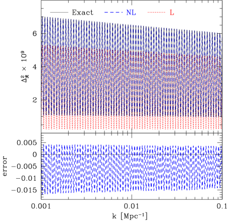
We now compare the analytic predictions with the exact calculation for example cases. In order to better separate out small effects that would be captured by the running of slow roll parameters from the new effects associated with nonlinear excitations, we evaluate the parameters of the template forms as follows. While Eq. (85) for the field position does not include running of slow roll parameters, we can enhance the accuracy of these calculations by choosing the normalization point $\phi_{*}$ as well as the calculation of $\omega$ and $A$ separately for each mode. As discussed in Ref. Motohashi and Hu (2015), for $\omega>1$ the optimal point is the resonance point where $x_{*}=k\eta(\bar{\phi})=\omega(\bar{\phi})/2$. We identify the resonance point by solving this equation where in practice rather we calculate $\bar{\phi}(\ln\eta)$ by convolving the field position $\phi(\ln\eta)$ with a Gaussian of width of order the resonance $\Delta\ln\eta=\sqrt{2/\omega}$ in order to remove the small oscillatory effects.

Likewise, when computing $\bar{\Delta}_{\cal R}^{2}(k)$, we use the exact solution on the $A=0$, $V=\bar{V}$ slow roll potential at the same field value at freezeout for each $k$-mode. Finally we use the full evaluation of $\varphi$ or ${\chi}-\psi$ in the analytic formulae rather than the Taylor expansions in Eq. (111), (112) around $k_{0}=0.05$ Mpc^-1. Thus deviations of the predictions from the exact calculation even at the level of the currently observationally negligible ${\cal O}(n_{s}-1)^{2}$ can be attributed to effects from the excitations rather than slow-roll evolution.

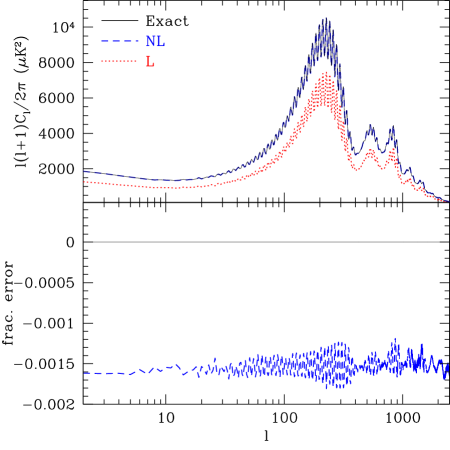
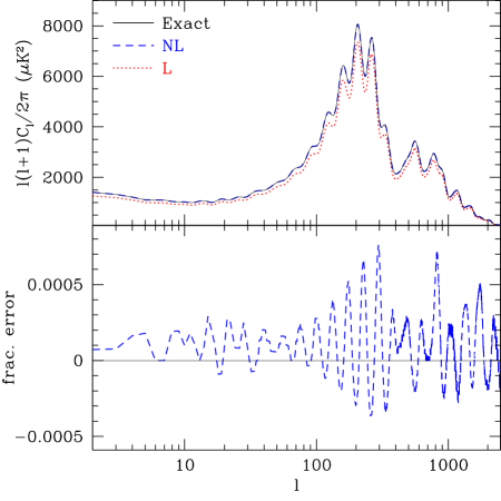
In Fig. 5 we show an example with a very high frequency $f_{a}^{-1}=1000$ or $\omega\approx 100$ and amplitude $A\approx 0.9$. Here and below we choose $\lambda=2.9609\times 10^{-10}$ and $\theta=0.59726$ for definiteness. Using the NL template form, the oscillation amplitude $\delta n_{s}=0.723$ and is near the edge of the region searched in Ref. Ade et al. (2015). Note that the NL template parameters predict the oscillation amplitude, phase and zero point in the curvature power spectrum to high accuracy (upper panel). Using the linearized form errs in all three quantities as expected even after removing slow roll drifts as described above. In the CMB temperature power spectrum, the oscillation amplitude is reduced by projection effects leaving the change in the zero point or effective scalar amplitude even more apparent (lower panel). Fractional errors in the oscillatory part for the NL template are comparable to or smaller than the cosmic variance limit all the way through the CMB damping tail. In fact we shall see that the main source of error can be removed by making small adjustments to the template parameters $B$ and $\varphi$ that merely change their association with the underlying potential amplitude $\Lambda^{4}$ and phase $\theta$ by a comparable amount.

Figure 9: Template parameter adjustment and template breaking terms for the high frequency $\omega\approx 100$ monodromy model of Fig. 5. Shown are the $\Delta_{\cal R}^{2}$ errors vs the exact computation with the analytic template parameters $B,\varphi$ (dashed), best fit template parameters (dotted), and the full fit including $C_{20},C_{22},\phi_{2}$ (long dashed). Most of the error is removed by the template readjustment which uncovers a much smaller offset, double frequency component that breaks the form of the high frequency template. The error after fitting this term is reduced to an entirely negligible level.

Figure 10: Template parameter adjustment and template breaking terms for the moderately high frequency $\omega\approx 25$ monodromy model of Fig. 6. Curves are the same as in Fig. 9.

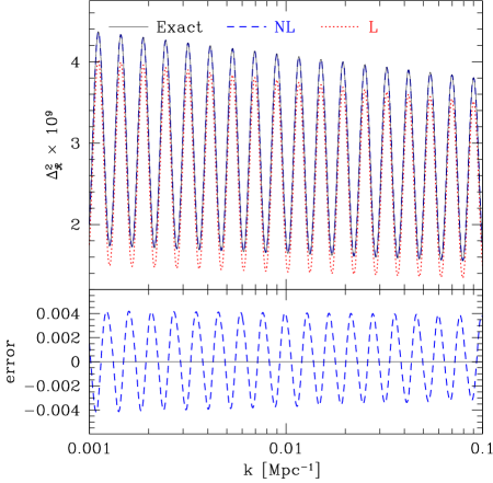
In Fig. 6 we show an example with a more moderate frequency $f_{a}^{-1}=250$ or $\omega\approx 25$ and a smaller amplitude $A\approx 0.45$. The smaller amplitude is chosen both because the smaller projection effects make oscillations in the CMB temperature power spectrum more prominent and because in our approximations we assume $A/\sqrt{\omega}\ll 1$. For this lower amplitude, we achieve comparable precision in both the curvature and temperature power spectrum as in Fig. 5.

To further test the accuracy of the NL template approximation we can fit for the oscillation amplitude, phase and zero point across a wide range in $A$ and $\omega$ and compare them with the predictions. First we consider $B$, $\varphi$, to be fit parameters at each $A$, $\omega$ for the exact power spectrum near $k_{0}$. In order to better capture the effects of the evolution of these quantities away from $k_{0}$ across several oscillations, we use the close agreement with the analytic forms to fit $B_{0}$, $\Delta\varphi_{0}$ and $\Delta\alpha_{\omega}$ as

$$B(k) = B_{0}\frac{B^{(\rm an)}(k)}{B^{(\rm an)}(k_{0})},$$

$$\varphi(k) = \varphi^{(\rm an)}(k)+\Delta\varphi_{0}+\Delta\alpha_{\omega}\ln(k/k_{0}).$$ (113)

We also fit the terms $C_{20}$, $C_{22}$ and $\phi_{2}$ in Eq. (III.2.4) to quantify the frequency suppressed terms that break the nonlinear template. Note that though $C_{20}$ violates Eq. (61), it can be reabsorbed into a change in $A_{s}$ and $\delta n_{s}$ in Eq. (109) whereas $C_{22}$ would break either template.

Figure 11: Template breaking offset double frequency components for the moderately high frequency $(\omega\approx 25)$ monodromy case. The estimates of Eq. (107) are $\sim 4$ times too high but otherwise usefully capture the scaling with $A$ and $\omega$.

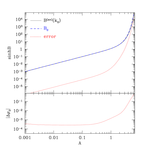
In Fig. 7, we show the result for an extremely high frequency ($f_{a}^{-1}=2500$, $\omega\approx 250$). This is near the highest frequency that is under control in the effective theory that underlies the calculation Behbahani et al. (2012); Adshead and Hu (2014). Remarkably, even when the oscillation amplitude reaches $\sinh B\approx 10^{3}$, or a thousand times the slow roll power spectrum, the analytic approximation for the amplitude and phase are accurate to a fraction of their values. This is consistent with the estimate from the quartic and quintic terms in Eq. (105).

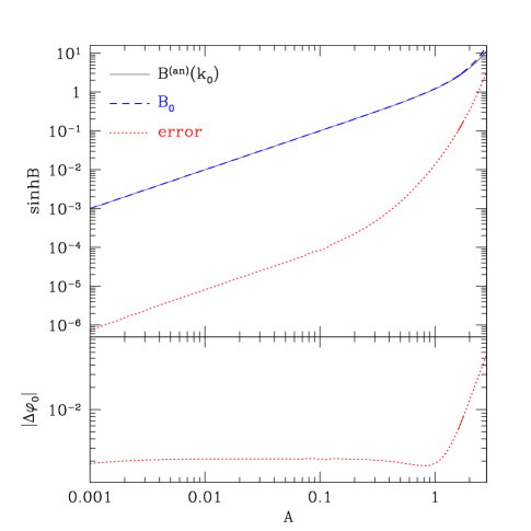
In Fig. 8, we show the same comparison for the moderately high frequency ($\omega\approx 25$) case. Due to neglected terms at low frequency in the model of Eq. (87), the good agreement extends out to a smaller $\sinh B\approx 10$ which is still an order of magnitude larger oscillation amplitude than the slow roll power spectrum.

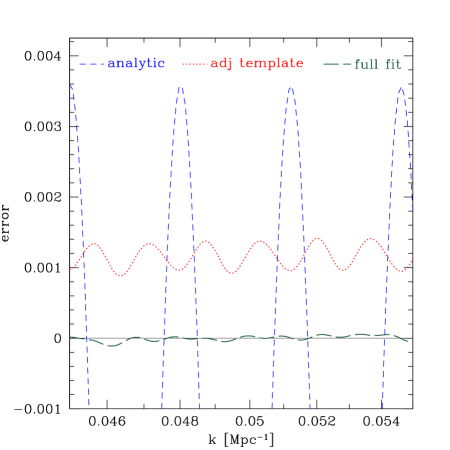
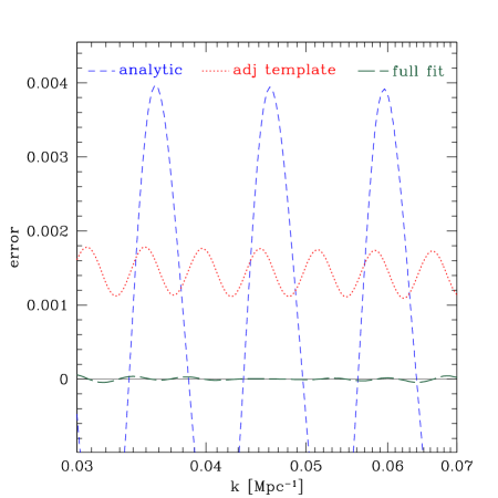
These fits also uncover the offset double frequency terms in Eq. (III.2.4). In Fig. 9, we show the breakdown of the errors in the analytic $\Delta_{\cal R}^{2}$ approximation in the high frequency model of Fig. 5. Once $B$ and $\varphi$ are adjusted with the fitted values of $B_{0}$, $\Delta\phi_{0}$ and $\delta\alpha_{\omega}$, the remaining errors are reduced by an order of magnitude and are of the form of an offset double frequency component. These fit well to the functional form given by $C_{20}$, $C_{22}$ and $\phi_{2}$ leaving the errors in the full fit at a negligible level.

These terms are not part of the high frequency template (61) and their contributions increase at lower frequency for a fixed $A$ at roughly the rate expected from Eq. (107). However due to projection effects, the same level of CMB temperature fluctuations requires a smaller $A$. For the moderate frequency and amplitude model of Fig. 6, the template breaking effects are at a comparable level (cf. Figs. 9,10). More generally we expect that for observationally viable models these terms which are neglected in the template form of fits to CMB data should make little to no impact on current constraints.

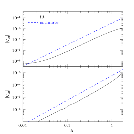
The rough estimate of Eq. (107) can provide a useful guide for deciding when in the future these terms would need to be considered. In Fig. 11, we compare these estimates to the fitted values of $C_{20}$ and $C_{22}$ for the moderately high $(\omega\approx 25)$ case. Eq. (107) overestimates these effects by roughly a factor of 4 but otherwise usefully captures the scaling for $0.03\lesssim A\lesssim 1$ and few $\lesssim\omega\lesssim 100$. For $\omega\lesssim 1$ the fully analytic results from Ref. Motohashi and Hu (2015) can instead be applied to quantify accurately these double frequency terms.

IV Discussion

In this work we have introduced a new formalism to calculate features in the curvature spectrum to arbitrary order in their deviation from the scale-free slow roll form. It improves on previous techniques involving the inflaton modefunction Stewart (2002b) by allowing a straightforward iteration that conserves curvature fluctuations order by order. This is important for models with order unity curvature features and larger where the iterative series must be resummed into a nonlinear form or where precision measurements require higher than second order accuracy.

Using these techniques, we show that for high frequency, or subhorizon, excitation of the curvature modefunction by features, the relationship between Bogoliubov excitation coefficients restricts the nonlinear form of power spectrum features. Due to this relationship, the first nontrivial effect of subhorizon excitations generating further excitations arises at third order. We show that if this process occurs contemporaneously with the original excitation, then the series can be resummed in closed form and is a simple exponentiation of the linearized response. Even for cases where this exact relationship does not hold, this exponentiated form provides a physically motivated and controlled template for fitting features in the power spectrum. It furthermore exactly matches second order perturbation theory in the small feature, high frequency limit. It improves on a similar exponentiation ansatz in Ref. Dvorkin and Hu (2010a) by enforcing the nonlinear relationship between the Bogoliubov excitation coefficients.

Applied to the step and axion monodromy models, these techniques greatly improve the accuracy of predictions for curvature and CMB temperature power spectrum features directly from potential parameters. In the step case, the improved form of the template allows greater than order unity curvature oscillations to be fit to better than cosmic variance accuracy for CMB measurements out through the damping tail. For monodromy, the improvement is mainly in the mapping between potential parameters and phenomenological parameters that describe the amplitude, phase and zero point of the logarithmic oscillations. Remarkably, our analytic description reproduces all three to good approximation even when the oscillation amplitude is $10^{3}$ times the slow roll power spectrum for models with sufficiently high frequency. Of course, this relates only to the formal accuracy of solutions to the Mukhanov-Sasaki equation (1), whereas correct predictions also require the validity of the effective theory that underlies it. We also estimate when terms that produce double frequency oscillations, which are absent in the subhorizon template, should be included when analyzing data.

These techniques will enable future studies of CMB and large scale structure power spectra to extend to high amplitude, high frequency features in specific cases such as steps and axion monodromy as well as in model-independent searches for temporal features during inflation.