The M 4 Core Project with HST - IV. Internal Kinematics from Accurate Radial Velocities of 2771 Cluster Members

Abstract

We present a detailed study of the internal kinematics of the Galactic Globular Cluster M 4 (NGC 6121), by deriving the radial velocities from 7250 spectra for 2771 stars distributed from the upper part of the Red Giant Branch down to the Main Sequence. We describe new approaches to determine the wavelength solution from day-time calibrations and to determine the radial velocity drifts that can occur between calibration and science observations when observing with the GIRAFFE spectrograph at VLT.

Two techniques to determine the radial velocity are compared, after a qualitative description of their advantages with respect to other commonly used algorithm, and a new approach to remove the sky contribution from the spectra obtained with fibre-fed spectrograph and further improve the radial velocity precision is presented. The average radial velocity of the cluster is $\langle v\rangle=71.08\pm 0.08$ km s^-1 with an average dispersion of $\mu_{v_{c}}=3.97$ km s^-1. Using the same dataset and the same statistical approach of previous analyses, 20 additional binary candidates are found, for a total of 87 candidates. A new determination of the internal radial velocity dispersion as a function of cluster distance is presented, resulting in a dispersion of $4.5$ km s^-1 within 2$\arcmin$ from the center of cluster and steadily decreasing outward. We statistically confirm the small amplitude of the cluster rotation, as suggested in the past by several authors. This new analysis represents a significant improvement with respect to previous results in literature and provides a fundamental observational input for the modeling of the cluster dynamics.

1 Introduction

M 4 (NGC 6121) is one of the most studied Galactic Globular Clusters (GGC). Its proximity, brightness and the moderate concentration make possible the study of its inner regions in great detail. This cluster has been the object of several intensive photometric campaigns, both from space (e. g. Bedin et al. 2013, Paper I, Piotto et al. 2015) and from the ground (e. g. Kaluzny et al. 2013, Libralato et al. 2014). Red giant members of this cluster are accessible to high-resolution spectroscopy with even medium-size telescopes, resulting in a wealth of abundance studies (e. g. Brown & Wallerstein 1992, Ivans et al. 1999, Smith & Briley 2005, Yong et al. 2008, Marino et al. 2008, D’Orazi et al. 2013), which have also provided evidences of multiple populations. Only recently the presence of multiple populations has been photometrically observed in the Red-Giant Branch (RGB) (Monelli et al., 2013) and in the Main Sequence (MS) (Milone et al. 2014, Paper II, Nardiello et al. 2015) This cluster also represents a natural benchmark for many theoretical studies, such as numerical simulations of the internal dynamics (Heggie & Giersz, 2008; Heggie, 2014) and the interactions with the Galaxy (e. g.  Dinescu et al. 1999).

Despite being so well-studied, the internal dynamics of this cluster are still poorly known. The kinematics of other GGC’s have been explored in more detail. One purpose of such studies has been to determine the presence of a central intermediate-mass black hole in a cluster center, using integral-field spectroscopy to measure the radial velocity dispersion in the center of the cluster (e.g. within 10$\arcsec$; see for example Feldmeier et al. 2013, Lützgendorf et al. 2013), Theories of gravity have also been tested by measuring radial velocities of individual stars in the outer regions of a cluster (farther than 1$\arcmin$ from the center of the cluster, see for example Baumgardt et al. 2009, Ibata et al. 2011). Both techniques have their disadvantages when determining the kinematical status of a cluster: integral field spectroscopy requires a deconvolution of the observed spectra along the line of sight, while results from individual stars may be hampered by the low statistics, especially near the center of far clusters where it may hard to observe individual stars.

M 4 represents an excellent target for kinematic analysis, thanks to its proximity and the many detailed studies of its properties. Still, the latest determination of the internal radial velocity dispersion as a function of distance dates back to the radial velocity study of Peterson, Rees & Cudworth (1995, hereafter P95) , which sampled 182 members with radial velocity precision 1 km s^-1. Despite the many recent spectroscopic campaigns on M 4, more precise and accurate wavelength calibrations are required for radial velocity determination than for chemical analyses. Spectra obtained for abundance studies may be affected by systematic shifts in radial velocity among different observations, or simply lack the required spectral resolution for a precise determination of velocities. These aspects are usually not important for chemical analyses, but they severely impact the use of spectroscopic data from different instruments for detailed kinematics analyses.

During last decade our group has collected thousands of spectra using the GIRAFFE spectrograph at VLT to estimate the geometrical distance, by comparing the radial velocity dispersion with the proper motion dispersion, and dynamical state of several GGC. Analyses of these spectra have been hampered by systematics in data calibration and radial velocity measurements; see for example Milone et al. (2006) and Sommariva et al. (2009; hereafter S09).

This project is the spectroscopic counter-part of an extensive astrometric and photometric investigation of M 4, involving about 700 WFC3/UVIS and 120 ACS/WFC HST images (GO-12911, PI Bedin), aimed at searching for and characterizing the binary population in the core as well as in the outskirts of the cluster (Bedin et al. 2013, Paper I for a careful description of the HST large program GO-12911).

In this paper we have focused our attention on significantly increasing wavelength calibration accuracies and radial velocity determinations of very low SNR stellar spectra. After introducing the dataset in §2, we devote §3 to a detailed description of the improvements in wavelength calibration. Our methodology to properly account for the geometrical distortions in a CCD chip when determining the drift in radial velocity that may occur between day-time calibration and science observations is described in §4. In §5 three well-known techniques are compared in order to establish which one is the most suitable to the characteristics of the instrument.

Finally, in §6 we discuss the application of these improved data reduction techniques to a dataset comprising 7250 spectra obtained with GIRAFFE for 2771 stars of the GGC M 4 in the wavelength region $5145-5360\,$Å. Only about 300 stars in our sample reside on the RGB. The vast majority of the stars are members of the Sub-Giant Branch (SGB) and MS stars, i. e. relatively faint targets with low SNR spectra. Careful consideration of the continuum placement and the sky contribution for each stellar spectrum is required. These aspects have already been discussed in Malavolta et al. (2014; hereafter LM14). While in our previous work we focused on the determination of atmospheric parameters over a wide range of evolutionary states and spectra of different quality, in this paper we aim to increase the precision of the radial velocities available in the literature and provide new insights into its internal kinematics.

2 The Spectroscopic Data Set

The spectra for our project were originally used by S09 to study the internal velocity dispersion of M 4 and to search for spectroscopic binaries. As described in LM14, the instrumental configuration was the GIRAFFE medium-high resolution spectrograph fed by the VLT Fibre Large Array Multi Element Spectrograph (FLAMES; Pasquini et al. 2000) in MEDUSA multi-fibre mode. This configuration produced single-order spectra for 132 objects (target stars and sky) in each integration. Using the GIRAFFE HR9 setup yielded spectra with dispersion of 0.05 Å/pixel and measured 4-pixel resolving power R $\equiv$ $\lambda/\Delta\lambda$ = 25,800 in the wavelength range $5143$Å $<\lambda<5356$Å. The HR9 wavelength region is particularly useful for radial velocity studies because it contains a large number of iron lines and very strong absorption lines, notably the Mg-b triplet.

The M 4 target stars were selected by S09 from an astrometric and photometric catalog based on Wide Field Imager (WFI) data from the ESO/MPIA 2.2m telescope Anderson et al. (2006). Each fibre’s radius on the sky is 0.6$\arcsec$, so each chosen star was constrained to have no bright neighbors (defined as $V_{neighbor}<V_{target}+2.5$) within an angular distance of 1.2$\arcsec$.

The spatial distribution and photometric properties of our target stars are the same as illustrated in Fig. 1 and 2 of LM14. Our target stars essentially sample all of M 4 spectroscopically up to twice the half-mass radius. The limiting magnitude of the targets, $V\lesssim 17.5$, was chosen to ensure that a single M 4 integration had signal-to-noise $\textrm{\mbox{SNR}}>10$ for each star, which was considered by S09 to be the minimum threshold to determine radial velocities (RVs) with a precision of a few hundred m s^-1, on the basis of previous experience with the instrument.

A total of 2771 stars covering CMD positions from the upper red-giant branch to about one magnitude fainter than the main-sequence turnoff (TO) luminosity were observed between 2003 and 2009, including 306 new spectra obtained in 2009 and targeting MS stars already observed in the previous epochs. Determination of the M 4 velocity dispersion and binary star fraction were the prime motivators for obtaining these data. Therefore nearly all stars were observed at least twice, and three or more spectra were obtained for nearly 40% of the sample. A total of 7250 individual spectra were available for our study, as we summarize in Table 1.

Table 1: Spectroscopic Observation Statistics

No. Observations	No. Stars	No. Total
1	83	83
2	1722	3444
3	501	1503
4	321	1284
5	72	360
6	20	120
7	1	7
8	27	216
9	10	90
10	12	120
11	1	11
12	1	12
Total	2771	7250

Default basic reductions (bias and dark correction, flat fielding) have been performed with the ESO pipeline. Spectral extraction has been performed using the optimal spectral extraction algorithm (Horne, 1986) and the empirical point-spread function concept from photometry (Anderson & King, 2000; Anderson et al., 2006) adapted to spectroscopy (LM14). The extracted spectra are fully consistent with the ones delivered by the ESO pipeline using either the HORNE option or the standard SUM, as a consequence of the fact that scattered light and fiber cross-talk are negligible in this specific setting of the MEDUSA mode. Wavelength calibration is performed by taking a hollow cathode Thorium-Argon lamp (hereafter simply Th-Ar lamp) spectrum with each of the fibres in the MEDUSA plate with the selected instrument setup. These standard calibration frames are usually taken during the day, several hours before observations. During a science exposure five fibres called simultaneous calibration fibres (SimCals) can be dedicated to take additional Th-Ar spectra, in order to correct for changes in the wavelength dispersion solution caused by variations in air pressure and temperature occurred inside the spectrograph between the day-time calibration and night observations. S09 used the ESO Giraffe standard reduction pipeline (Blecha et al., 2000) and the Ancillary Data Analysis Software (Royer et al., 2002) to reduce the M 4 data from raw CCD exposures to wavelength-calibrated 1D spectra, apply the drift correction in the wavelength scale and determine the radial velocities of the observed stars.

A systematic offset of 150 m s^-1 in the radial velocity zero point was observed by in the five simultaneous calibration fibres between 2003 and 2006 data (see §4.1 of S09 for a detailed discussion). Changes in environmental conditions inside the spectrograph (i. e. air pressure and temperature), as well as switching to different instruments modes, could cause an overall shift in wavelength (and hence RV) in the interval of time between observations and calibration exposures and between different nights. These should be automatically taken into account by the ESO pipeline using the simultaneous calibration fibres. After removing this source of systematic error, the only expected variation in RVs of calibration spectra taken in different epochs should have a random distribution, given by the precision in RV of the spectrograph and independent with time.

The dispersion inside a single epoch is several times smaller then the offset (Fig. 6 of S09), and this seems to imply a problem in the original wavelength dispersion solution. Therefore we decided to revisit the basic reductions of the raw data sets, to see if the velocity precision could be significantly improved. In the next sections our different approach to wavelength calibration and drift correction is described. To mark the difference with the ESO pipeline, we will refer to our approach as Direct Calibration.

3 GIRAFFE Wavelength Calibration

ESO provides a pipeline for GIRAFFE as a part of the VLT Data Flow System (DFS). A detailed description of the pipeline can be found at the ESO website; here we provide a brief description of the wavelength calibration subroutine to highlight the differences with our Direct Calibration technique.

3.1 ESO Pipeline calibration

Calibration frames used for dispersion solutions are obtained by illuminating the entrance of the fibres with a hollow cathode Th-Ar lamp using the same setup as for the stellar spectra. A complete GIRAFFE dispersion solution consists of an optical model of the fibre spectra onto the CCD detector, a polynomial fit of the optical model residuals, and the correction of individual fibre offsets.

The solution is determined iteratively, i. e. at each iteration the previous model is updated until the measured emission lines have a negligible radial velocity with respect to the tabulated values. A previous dispersion solution is useful for rapid computations, but, if necessary, a new dispersion solution can be computed from scratch using the average optical model that accompanies the pipeline software.

In detail, for each wavelength calibration procedure, a set of unsaturated Th-Ar emission lines is selected according to the instrumental setup of the images. The position of these lines on the CCD is determined using an analytical optical model. The residuals between these positions and the measured ones are then modeled with a 2D Chebyshev polynomial. The global wavelength solution is then the sum of the optical model and of the polynomial residuals. See Royer et al. (2002) for a detailed description of the ESO pipeline, and Bristow et al. (2010) on the use physical models for instrument calibration.

3.2 Direct Calibration

A more classical, direct approach has been followed in our work. For each individual Th-Ar spectrum, a selected list of emission lines with known wavelengths are measured and then a piecewise polynomial (represented as Basis spline, de Boor 1977) is fitted to determine the wavelength dispersion solution.

The algorithm presented here is designed to automatically perform those steps that in other tools such IRAF require human interaction. Although our reference wavelength range and resolution are the ones defined by the HR9 setting of GIRAFFE, we want to keep our algorithm as general as possible for rapid adaptation to different wavelength GIRAFFE ranges or for spectra obtained with different instruments.

3.2.1 Line lists of Thorium and Argon lines

Several published Th-Ar line lists are available in which lines have been selected according to their stability and strength from high resolution spectra; see for example Murphy et al. (2007); Lovis & Pepe (2007). However, when dealing with medium resolution spectroscopy, blending with close or faint lines becomes important. The centers of lines of interest can be shifted several hundredths of Ångstroms, thus leading to a less precise determination of the wavelength dispersion even with excellent data and a very accurate line list.

To create a line list that takes into account line blending, we proceeded in the following way. We have selected the Th-Ar reference spectrum obtained with ESO’s 3.6m telescope Coude Echelle Spectrometer (CES, Enard 1982) as our reference among several Th-Ar spectrum available in the literature after checking the similarity with GIRAFFE Th-Ar spectra (emission features may change depending on the manufacturer of the lamp). This spectrum has been obtained with a resolving power of $R=200,000$, which is almost nine times the resolving power of GIRAFFE in the HR9 setting. We degraded this spectrum to match the resolution of our spectra; we will refer to this smoothed spectrum as the reference one. All the calibrations will be relative to the reference system given by this spectrum.

Lines have been automatically identified using the first derivative of the reference spectrum. Fig. 1 shows an example of the line identification process, with the smoothed reference spectrum in the upper panel (in arbitrary units $f$) and its first derivative in the lower one (in arbitrary flux units per Ångstrom $f$Å^-1). To separate strong lines from small features and weak emission lines, we have selected only lines with null derivative at the expected central wavelength and inflection points on the side that have a minimum absolute value of 100 $f$Å^-1.

Figure 1: An example of the line identification on the Thorium-Argon reference spectrum, with the smoothed spectrum in the upper panel and its first derivative in the lower one. Very weak lines have been excluded in our analysis if the inflection points of their first derivative are within the two blue dashed lines. Selected lines are denoted by a red vertical line.

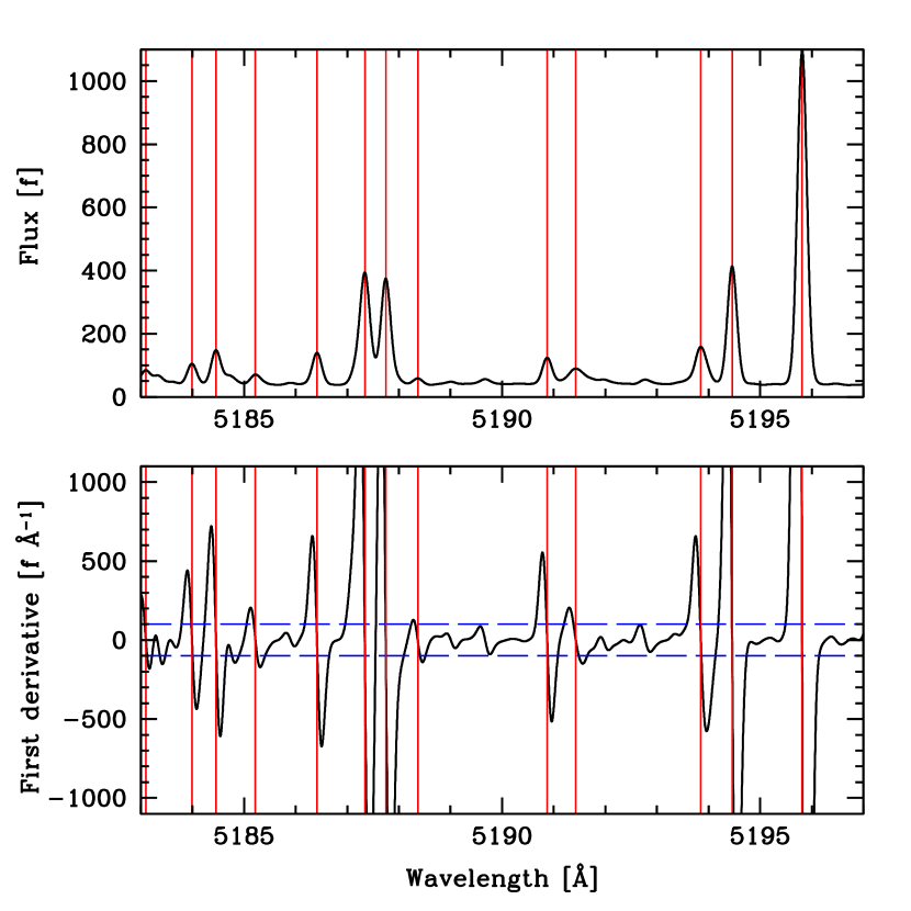
In our wavelength range 178 lines have been identified. The positions of these lines have been measured on the reference spectrum, and their values define our rest-frame system of reference for the determination of the wavelength dispersion solution of GIRAFFE calibration spectra.

3.3 First approximation of the wavelength dispersion solution

A first approximation to the dispersion solution is needed to allow the algorithm to determine the solution.

We start by selecting the ten lines with the largest fluxes from the reference Th-Ar spectrum in the wavelength range of interest. The number of lines has been chosen in a way that the included lines form a subset with mean flux that is at least a few times the flux of the brightest lines not included in the subset. This ensures that the selection in the observed spectra will not be affected by differences in the line flux ratios that may be present when comparing spectra obtained with lamps made by different manufacturers. A very rough pixel position for each line must be provided also: a single value is good enough for all the fibres, despite their shift in the cross-dispersion direction. The wavelength values are used as initial guesses for a Gaussian fit, so a precision of one half of the full-width-at-half-maximum (fwhm) is good enough. This selection can be easily performed by visual inspection directly at the reference spectrum, and must be done only once for a given wavelength range or instrument setup. This is the only human interaction required by the algorithm.

A Gaussian fit on these pre-selected lines is performed on both the pixel space for the observed spectrum and in the wavelength space for the reference one. The values are sorted in increasing order, so that the values in the pixel space have now an associated wavelength. The only precaution to be taken at this step is to check that no strong lines are present close to the border of the wavelength range (e. g. $10$ Å from each limit for our instrument setting), otherwise an error in the association of lines with pixels can occur. In fact, as a result of the optical design of GIRAFFE, the wavelength range of the spectra varies slowly across the CCD, with a maximum shift of about $10$ Å for the fibres close to the center of the sensor respect to the first one.

Before proceeding to the first approximate determination of a wavelength solution, we need an additional step to ensure that cosmic rays or uncorrected hot pixels have not been identified as spectral lines. By inspection of our data frames, we noticed that real spectral lines have a total shift of around 100 pixels in the cross-dispersion direction (i. e. across the fibres). The maximum shift with respect to the first fibre around the center of the frame is 50 pixels, so we set this value as a threshold for checking proposed line identifications in the various fibres. This steady shift in line positions in different fibres is a consequence of the optical design of the instrument and it varies smoothly across the sensor, so for each wavelength value we perform a low-degree polynomial interpolation of the pixel values versus their fibre number. The fit is performed a second time after the removal of outlier pixel values. The approximate wavelength solution is finally obtained interpolating the wavelength values versus the corresponding pixel values with a low-order polynomial (degree=3)

3.4 Wavelength dispersion solution for a single frame

Now that an approximate solution is available, the determination of the final dispersion solution is an iterative process where the resulting precision is increased with each iteration. These are the steps that we followed:

• at each iteration more faint lines are measured in the calibration frame and associated with lines in the reference spectrum.

• Lines with fwhm higher then a given threshold, nominally twice the instrumental fwhm at that wavelength, are excluded from the list;

• The dispersion solution is computed again, and the order of the polynomial can be increased according to the number of added lines.

• Lines that have an interpolated wavelength that differs from the reference value over a given threshold are rejected and not included in next iterations; the threshold is initially very large and it is rescaled at each iteration.

In the last two iterations, the lines are weighted according to their brightness and their width in both the calibration spectra and the reference one. After several tests Equation 1 was found to provide the best combination of these parameters,

$$w_{i}=\left(\sqrt{\sigma_{cal,i}^{2}+\sigma_{ref,i}^{2}}+500/\sqrt{A_{i}}\right)^{-1}$$ (1)

where $w_{i}$ is the weight associated to the line $i$, $\sigma_{cal,i}$ and $\sigma_{ref,i}$ are the widths of the line in the calibration and reference Th-Ar spectrum respectively, and $A_{i}$ is the measured amplitude of the line. An example of the weight association as a function of wavelength is given in the upper panel of Fig. 2 for a randomly selected calibration frame.

In the last two iterations, the polynomial function is substituted with a piecewise polynomial (in the form of Basis splines or B-splines). To fit the curve to our data we made use of the EFC routine included in the SLATEC Common Mathematical Library, a collection of mathematical and statistical routines written in Fortran 77. This procedure is repeated individually for each fibre.

Figure 2: Two quantities associated with pixel-wavelength calibrations are plotted as functions of wavelength. In the upper panel, the weight associated to each line is shown. In the lower panel, the difference between the wavelength determined using the dispersion solution for the measured center of the line, and the reference wavelength from CES spectra is plotted. The standard deviation of this difference is reported in the figure. Points from different fibres are color-coded accordingly.

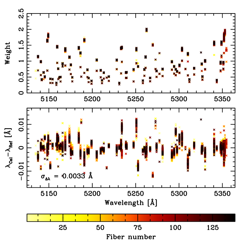
In the lower panel of Fig. 2 the difference between the wavelength obtained with the dispersion solution (from the position in the pixel space) and the reference wavelength from the CES spectrum is shown as a function of wavelength. The standard deviation of this difference, determined using all the lines measured in a calibration frame, is on average $\sigma=0.0033$ Å, which corresponds to $\simeq 1/15^{\textrm{th}}$ of a pixel.

3.5 Overall calibration

After the wavelength calibration of a frame, the lines used for the dispersion solution are stored. Our dataset span a large temporal range, from almost the beginning of the scientific observations of GIRAFFE in 2003 until 2009. The information on emission Th-Ar lines from all these frames is collected in order to identify a stable set of lines and improve the dispersion solution. Only the lines that have been successfully measured on $90\%$ of the fibres are retained. The only exception is for those lines that are closer than $10$ Å to the edge of the spectrum, for the reasons explained in §3.3. The weight associated to each line is the mean of the weights calculated in each calibration fibre using Equation 1. A total of 114 lines has been selected (Table 2). The dispersion solution is then computed again, using the same function of the last iteration in §3.4 but with the improved line list.

Table 2: Lines and Weights used for the Dispersion Solutions

n	Wavelength [Å]	Weight	n	Wavelength [Å]	Weight
1	5134.7457	8.776	58	5239.5502	8.574
2	5136.1202	26.557	59	5241.8563	30.608
3	5137.4775	15.334	60	5243.7542	24.384
4	5140.7642	13.070	61	5247.6542	9.685
5	5141.7838	5.382	62	5250.8742	18.822
6	5143.9137	8.399	63	5252.8043	11.150
7	5145.3047	6.584	64	5254.2542	12.568
8	5148.2122	19.641	65	5258.3603	4.827
9	5149.2102	21.811	66	5260.1046	9.866
10	5151.6104	5.564	67	5261.4763	15.428
11	5154.2434	5.420	68	5262.6055	23.083
12	5157.4512	26.060	69	5264.8003	19.409
13	5158.6042	3.818	70	5266.7102	6.025
14	5159.5911	19.307	71	5269.7842	19.385
15	5160.7159	9.8942	72	5272.9343	14.107
16	5161.5402	4.598	73	5274.1183	9.093
17	5162.2882	6.315	74	5277.4967	13.711
18	5163.4582	6.360	75	5281.0698	9.834
19	5164.4022	23.736	76	5282.4010	23.019
20	5165.7682	12.135	77	5283.6902	24.195
21	5166.6522	23.825	78	5286.8895	15.986
22	5168.9242	18.375	79	5289.9048	21.810
23	5170.2482	23.561	80	5291.8202	13.201
24	5170.2482	25.057	81	5294.3981	11.068
25	5173.6782	14.890	82	5295.0866	17.948
26	5175.3262	11.583	83	5296.2823	9.744
27	5176.9642	6.212	84	5297.7575	8.974
28	5178.4602	21.545	85	5300.5243	11.599
29	5180.7198	22.175	86	5301.4042	13.648
30	5182.5242	15.943	87	5303.4689	18.513
31	5184.4562	19.374	88	5305.6923	16.192
32	5186.4122	16.782	89	5307.4660	14.933
33	5187.3402	5.066	90	5309.6143	20.676
34	5190.8742	19.680	91	5310.2690	16.136
35	5194.4582	9.513	92	5312.0023	5.200
36	5195.8142	5.877	93	5315.2242	19.243
37	5197.2362	21.669	94	5317.4943	10.140
38	5199.1702	4.668	95	5320.7727	21.339
39	5202.0231	21.904	96	5322.9002	20.316
40	5203.8475	19.515	97	5325.4079	17.428
41	5205.1522	13.871	98	5326.2724	11.946
42	5206.5122	19.620	99	5326.9763	6.434
43	5207.7907	24.472	100	5329.3943	10.258
44	5209.7252	9.314	101	5330.0782	13.466
45	5211.2309	4.933	102	5333.3903	24.130
46	5213.3589	8.251	103	5337.0125	24.140
47	5216.6123	6.105	104	5338.2680	23.143
48	5219.1121	6.626	105	5340.5048	19.221
49	5220.9031	8.875	106	5343.5817	4.772
50	5226.5323	24.091	107	5345.3154	22.528
51	5228.2291	14.010	108	5346.3805	20.157
52	5228.9985	22.407	109	5347.9737	12.361
53	5231.1600	3.836	110	5349.0053	19.482
54	5233.2263	18.568	111	5351.1289	12.436
55	5234.1222	19.372	112	5351.8442	21.831
56	5237.9123	28.873	113	5353.0208	22.987
57	5238.8142	8.417	114	5354.6055	17.678

Figure 3: As in Fig. 2, on the same calibration frame but using the refined line list. Note the reduction in the standard deviation compared to the previous figure.

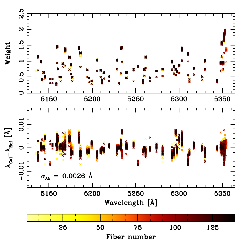
Using the same set of lines and weights to compute the dispersion solution results in a more homogeneous calibration of the entire dataset, while using the more stable lines reduce the scatter around the computed dispersion. In Fig. 3, the resulting overall calibration for the same frame in Fig. 2 is shown. A further reduction of the dispersion from $\sigma=0.0033$ Å to $\sigma=0.0026$ Å of the difference between measured and reference wavelength of individual lines is obtained. To have an idea of the goodness of the dispersion solution, this result can be compared with the average pixel size of $\simeq$0.05 Å, or typically $\lesssim 1/19^{th}$ of the size of a pixel.

4 SimCal calibration

A simultaneous calibration lamp provides a reference system obtained simultaneously with the observations, to take into account drifts of the spectrum in the wavelength space that may occur during the time between the Th-Ar lamp calibration frame and observations.

GIRAFFE has five fibres available for Th-Ar SimCal, homogeneously distributed between the science fibres. In the ESO pipeline, drifts are corrected by cross-correlating the SimCals with the provided numerical mask; the resulting offsets are linearly interpolated across the CCD in the cross-dispersion direction to determine the wavelength offset to be applied for each fibre to the dispersion solution obtained using the day-time calibration frame. Two apparently reasonable assumptions are made here: the drift is constant in the velocity space across the wavelength range of the considered order, and that the overall shift is linear in the spatial direction of the CCD.

We first check if these two assumptions are correct. In order to do so, we need to compare two Th-Ar calibration frames with a measurable drift. We then opted to compare calibration frames from two different nights. Emission line positions for each fibre are measured in both frames and the difference in pixel space is taken. Conversion of differences from pixel space $\Delta x_{i}^{pixel}$ into radial velocity space $\Delta RV_{i}$ for the $i_{th}$ line is given by:

$$\Delta RV_{i}=\Delta x_{i}^{pixel}\delta\lambda(i)\ c/\lambda_{i}$$ (2)

with $\lambda_{i}$ given by the day-time wavelength dispersion solution, $\delta\lambda_{i}$ is the size of the pixel in the wavelength space at the position of the $i_{th}$ line.

Figure 4: Radial velocity shifts between the calibration frames of two typical nights, along the cross-dispersion direction. The position along the wavelength dispersion direction is color-coded. This plot shows that the common practice of assuming a constant value along one axis is not justified.

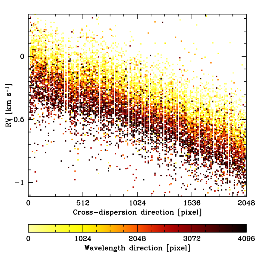
Fig. 4 and the first panel of Fig. 5 show the difference between the calibration frames of two typical nights. Different night combinations show similar results, with the only significant difference being the amount of overall radial velocity shift. It appears clear that both ESO pipeline assumptions here do not hold: the shift is not constant for a single fibre, and it is not a linear function of the cross-dispersion direction. Probably these differential shifts also happen during individual nights, even if in a less pronounced way. We conclude that correcting for a single value of the radial velocity will not provide a good correction for drifts, specially when temperature and air pressure inside the spectrograph are not actively controlled, as in our case.

Figure 5: First panel: Radial velocity shift of Th-Ar emission lines between the calibration frames of two different nights. Second panel: 2-D polynomial fit to the data of the first panel, using all the available fibres in the frame. Third panel: the same fit is performed using only the Simultaneous Calibration fibres. Radial velocity shifts are color-coded. The chosen model is able to reproduce the global shape of the RV shifts while using the SimCals alone, with little influence from outliers.

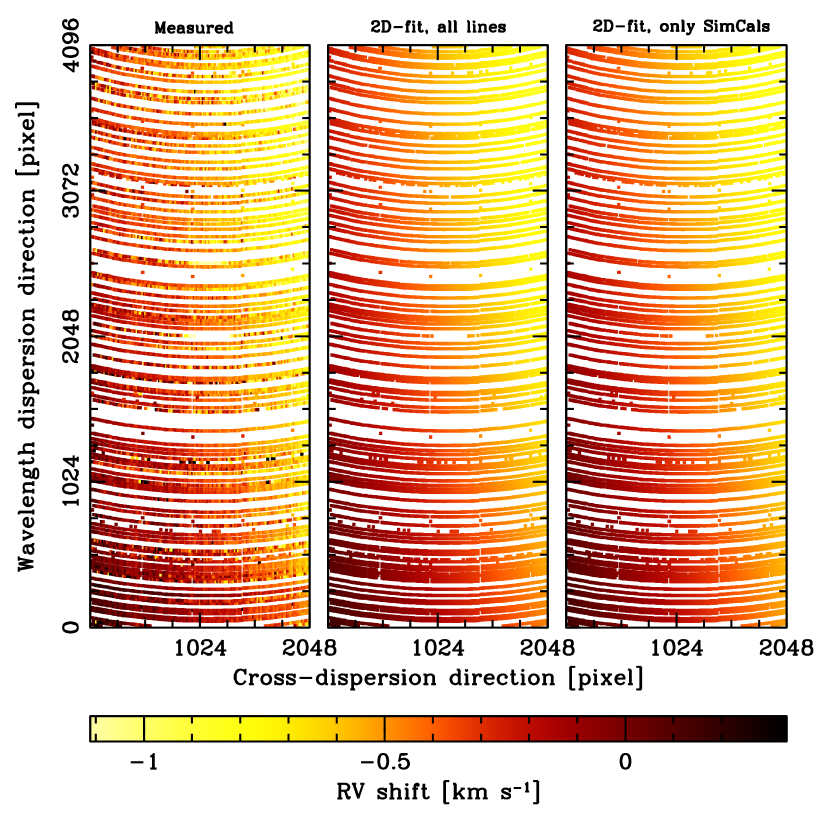
In our new analysis, a 2D polynomial fit (Chebyshev polynomials of the first kind) of degree $(2,2)$ has been chosen to model the shift in radial velocity as a function of pixel coordinates. However, during science observations only five fibres out of 132 are available for simultaneous calibration (fibres 1, 32, 63, 94 and 125). To check if the polynomial fit works as well with a reduced number of fibres, we performed two fits of the measured RV differences for two given nights (first panel of Fig. 5): the first one using all the available fibres (second panel of Fig. 5), and the second one using only the SimCals fibres (third panel of Fig. 5), in both cases using the same function to fit the measured differences.

Figure 6: First panel: differences between the SimCals drift model and the observed radial velocity shift. Second panel: differences between the SimCals drift model and the same model using all the calibration fibres. The same calibration frames of Fig. 4 and 5 have been used. The scatter in RV of individual lines is clearly larger than the error we introduce in the global determination of the drift by using only the SimCals fibres.

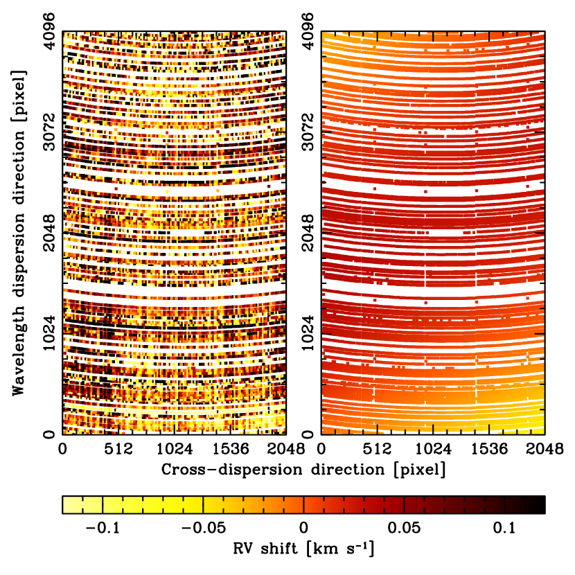
In the example shown in Fig. 6, the difference between the drift model using only SimCal fibres and measured line positions (left panel) has a mean of $\langle{\Delta_{RV}}\rangle$ $<$ 10 m s^-1 and standard deviation $\sigma\simeq 125$ m s^-1 after $5-\sigma$ clipping. The difference with the model obtained using all the fibres (right panel of Fig. 6) shows a systematic of $\langle{\Delta_{RV}}\rangle$ $<$ 10 m s^-1 and a $\sigma\simeq 20$ m s^-1 (after $5-\sigma$ clipping). Considering that we are using only 5 fibres out of 132 to redetermine the drift across the whole detector, this is a reasonable result. Finally, we note that polynomials with higher degrees resulted in fit too sensitive to outliers when using only the five SimCal fibres.

5 Radial velocity determination

In next section the three most popular techniques in radial velocity measurement are briefly described: Classical Cross-Correlation Function (CCF), Numerical CCF (nCCF), and Synthetic Template Matching. The steps for determination of radial velocities for each fibre within each exposure are then described in detail.

Classical Cross Correlation function: This is the technique developed by Tonry & Davis (1979) and implemented in the RVSAO package (Kurtz & Mink, 1998). The observed spectrum is rebinned into a linear scale in logarithmic wavelength, continuum normalized and then the Fourier power spectrum (FPS) is computed. The Fourier power spectrum of a pre-selected template spectrum is computed too, and the two FPS are cross-correlated to determine the radial velocity shift. In some modifications of the algorithm, the CCF is computed using the spectra directly, in the log-wavelength space.

Numerical CCF: This is the technique introduced by Baranne et al. (1996) and improved by Pepe et al. (2002), also known as CORAVEL-type CCF. The observed spectrum is cross-correlated in wavelength space with a numerical mask with non-negative values at the central position of the line, and zero otherwise. Each value of the mask, or weight, is determined using a synthetic spectrum, taking into account the depth of the line and its width, in order to optimize the extraction of the doppler shift information. The cross correlation function is constructed by shifting the mask as a function of the Doppler velocity, and integrating the product of the mask with the observed spectrum. As a result of this definition, the value of the RV is given by the minimum in the cross-correlation function. To avoid confusion we will refer to this definition as nCCF This technique has proven its reliability in the discovery of several exoplanets, and achieves best results when a large number of lines is available (e. g., Pepe et al. 2004).

Synthetic Template matching: A synthetic spectrum to be used as rest-frame reference is generated using the atmospheric stellar parameters from photometry. The observed spectrum is shifted in the RV space and for every shift $v_{r}$ the $\chi^{2}$ of the difference between the observed and the synthetic spectrum is computed. The value of $v_{r}$ that gives the lowest $\chi^{2}$ is taken as the radial velocity of the star.

The main disadvantage of Classical CCF technique is that the rebinning process (required for the FPS computation) can introduce correlated noise in cases of very low SNR spectra. Since we want to avoid spectra rebinning in the first place this technique and further derivation have not been considered in the following analysis.

5.1 Application of the numerical techniques

We describe now our implementation of the Synthetic Template matching technique. To begin, the sky spectrum is removed from the observed one and the result is normalized to the continuum level of the stellar flux as later described in §5.2. Instead of a $\chi^{2}$ function, we minimize the least-square function LSQ defined in Equation 3, where $f_{\star}$ is the observed stellar spectrum (after the steps described above), $f_{\textrm{syn}}$ is the synthetic one, and the sum is over the $n_{pixel}$ data points of the observed spectrum. Pixels affected by cosmic rays or CCD defects and spectral ranges contaminated by Th-Ar emission from close SimCals fibres are flagged with a zero value in $mask$, and unitary value otherwise.

$$LSQ(v_{r})=\sum_{i}^{n_{pixel}}\left(\frac{f_{\star}(i)-f_{\textrm{syn}}(i,-v_{r})}{1.2+f_{\textrm{syn}}(i,-v_{r})}\right)^{2}mask(i).$$ (3)

For each determination of the $LSQ$ function the synthesis is shifted by $-v_{r}$ in the radial velocity space (in the opposite direction since $v_{r}$ is the velocity associated to the star) and then rebinned into the wavelength scale of $f_{\star}$. This approach avoids the more problematic rebinning of the noisier observed spectrum, and is the reason why the dependence on $v_{r}$ has been included in the synthetic spectrum $f_{\textrm{syn}}(i,-v_{r})$.

The denominator of Equation 3 differs significantly from the one of a standard $\chi^{2}$ function. We did not include the dependence on the continuum in $LSQ$ determination because this shape is changing with time and changes in instrumentation (e. g. the change of CCD in May 2008); thus it could have introduced a bias depending on the epoch of observations. We instead decided to divide by the synthetic spectrum to give more weight to spectral lines, while a constant has been added to avoid an excessive weight for the deepest lines. The value of the additive constant has been found empirically by performing several tests on a subsample of stars of different spectral kind and with multiple observations.

Figure 7: Comparison between the “CORAVEL-type” Numerical CCF (upper panel) and Synthetic Template Matching (lower panel) on the spectrum of a SGB star with $V=16.4$. The blue line represents Gaussian fits to these functions.

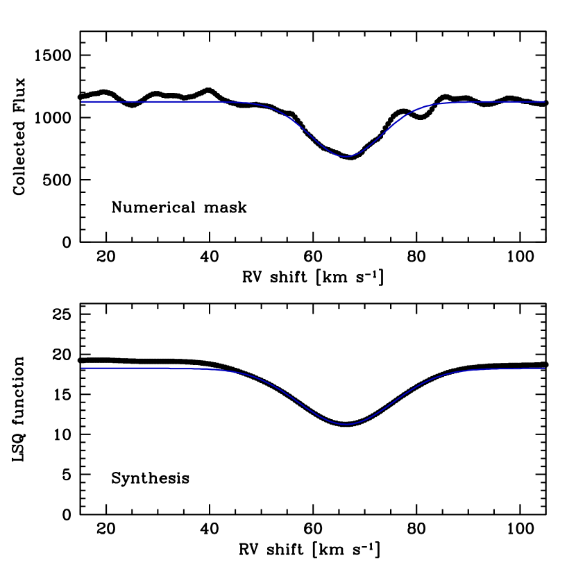
We have tested the Numerical CCF and the Synthetic Template Matching on several stars with spectra at various SNR to choose the technique that better suits our dataset. The resulting functions for a SGB star with $V=16.4$ are shown in Fig. 7 in order to show the differences between the two techniques. For a given value of the radial velocity the Numerical CCF technique is using only the portions of the spectrum that are falling inside the positive values of the mask (namely $\delta-$functions), while with the Synthetic Template Matching the $LSQ$ function is determined over the entire spectrum. In both cases the width of the resulting functions will be given by the sum in quadrature of the average width of the spectral lines in the observed spectrum and the width of the lines in the mask/synthesis, hence with the Synthetic Match technique the final functions will be broader with respect to the Numerical derived one. A broader function will result in a greater uncertainty in the determination of its center, i. e. the Synthetic Match delivers a less precise radial velocity than the CORAVEL technique (if the same linelist is used in both cases). On the other hand, while this may be true in an ideal situation, when the limited wavelength range of the spectra allows to use only a few hundred of lines (with respect to the thousands of lines as in Pepe et al. 2004) as in our case, the CORAVEL technique is too sensitive to noise, as exemplified in Fig. 7. We therefore decided to use the Synthetic Match to determine the RV of the whole set of stars.

5.2 Continuum normalization and Sky flux determination

Continuum normalization is one of the most daunting tasks in stellar spectroscopy. Generally speaking, there are several ways to deal with the continuum. When a spectrum has extended wavelength coverage as in the case of Echelle spectra, and the aim is to fit synthetic spectrum to the data, the continuum is obtained by fitting pre-selected feature-less spectral regions around the one to be analysed (as done by Kirby, Guhathakurta & Sneden 2008, but many other examples are available in literature). In other cases as in the case of Equivalent Width measurements the interest is focused on individual lines and it is possible to use those surrounded by at least a few Ångstroms of local continuum (see for example the criteria used by Sousa et al. 2007 to create their linelist).

Our dataset however presents several major complications. The spectral range is very short, $\Delta\lambda=214$ Å, and very crowded, so there are no line-free regions available to set a continuum level reliably. In fact, the HR9 setting was chosen for the richness in this spectral window. The wings of the Magnesium-I triplet ($5167.33$ Å, $5172.70$ Å, $5183.62$ Å) affect nearly one quarter of the spectrum beginning at the low-wavelength edge of our spectra, so that the continua must be extrapolated from the last three quarters of the spectra. Moreover, many lines are blended or very close, making the determination of local continua very difficult.

To determine the continuum for each spectrum, we used a technique similar to the one introduced in LM14. Briefly, the continuum level and sky contribution are determined by using a spectral synthesis, obtained using the photometric stellar parameters and average metallicity of the cluster, and the Solar Flux Atlas (Kurucz et al., 1984) as a template sky spectrum, both normalized to unity. Photometric atmospheric parameters for M 4 have been derived using the photometric catalog kindly provided by Peter B. Stetson (D’Antona et al., 2009) and the calibrations from Ramírez & Meléndez (2005) and Casagrande et al. (2010). The latest determinations for reddening and distance from Hendricks et al. (2012) have been adopted:  $E(B-V)=0.37\pm 0.01$, $R_{V}=3.62$ and $D_{\rm cluster}=1.80\,{\rm kpc}$. Syntheses are generated using the current version of the Local Thermodynamic Equilibrium (LTE) code MOOG (Sneden, 1973), and Kurucz (1992) atmosphere models calculated with the $\alpha-$enhanced New Opacity Function Distribution (AODFNEW, Castelli & Kurucz 2004). More details on the photometric parameter determination, atomic line parameters and synthesis calculation can be found in LM14.

To apply this technique, we need to know the radial velocity of the star. At this stage high precision in RV is not required. A single pixel has an average size of $2.5\,\mbox{km\,s${}^{-1}$}$, so an error of several hundreds m s^-1 still yields a good fit of the synthesis to the observed spectra, given the fact that our goal at this stage is to determine the continuum level and not to derive accurate radial velocities or stellar parameters. The radial velocity is derived using a numerical CCF (Baranne et al., 1996) with line positions and weight derived from the same synthetic spectrum that will be used to determine the continuum, following the prescriptions in Pepe et al. (2002).

$$nCCF(v_{r})=\sum^{i}nCCF^{i}(v_{r})=\sum^{i}\int_{\lambda^{i}_{v_{r}}-\delta\lambda/2}^{\lambda^{i}_{v_{r}}+\delta\lambda/2}f(\lambda)c^{i}d\lambda.$$ (4)

As can be seen from Equation 4, the value of the nCCF at a given radial velocity point $v_{r}$ is proportional to the sum of the stellar flux collected by each $\delta$ function $i$ in the numerical mask, rescaled for the weight $c_{i}$. In this equation, $\lambda^{i}_{v_{r}}$ is the wavelength of the line $i$ shifted for the radial velocity of the nCCF and $\delta\lambda$ is the size of the hole in the numerical mask.

Figure 8: In the top panel, the nCCF from the normalized spectrum of the synthesis (blue line) and the sky (red) are shown. In the bottom panel, $nCCF_{syn}$ and $nCCF_{sky}$ are rescaled according to the measured flux to show the relative influence, and their sum (green) is compared with the observed nCCF (black). A star with $V_{mag}=16.4$ is considered here as example.

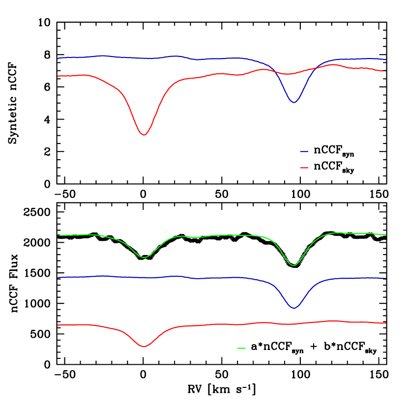
The result of the numerical CCF allows us to determine the star/sky flux ratio. The nCCF is computed for the smoothed synthetic spectrum ($nCCF_{synth}$) and the sky spectrum ($nCCF_{sky}$) without any further correction and using the same numerical mask. The cross-correlation function of the observed spectrum $nCCF_{star}$ is then fitted with a linear combination of $nCCF_{synth}$ and $nCCF_{sky}$, being the linear coefficients of the fractions of stellar and sky fluxes.

The upper panel of Fig. 8 shows the $\rm{nCCF}_{synth}$ (red line) and the $\rm{nCCF}_{sky}$ (blue line) derived from normalized spectrum. The sky spectrum has a lower continuum and a deeper nCCF because of the higher metallicity and lower temperature respect to the observed star. In the lower panel, the two nCCFs are rescaled according to their estimated fluxes in order to show their relative influence, and their sum (green line) is compared with the observed nCCF (black points). Note here that this technique works best when the observed RV of the star (including Earth motion contribute) differs significantly from the RV of the sky, i. e. $|v_{r}^{star}|>20$ km s^-1.

Both solar and synthetic spectra then are rebinned into the wavelength scale of the science spectrum (keeping constant the flux for wavelength unit) and degraded to match the spectral resolution of the instrument. Finally the instrumental effects (e. g.flat-fielding) are applied to make the comparison with the observed spectrum possible. A normalized linear combination of the two modified spectra, with the sky/flux ratio as coefficients, is multiplied by a polynomial function: its coefficients are determined by fitting the observed spectrum. The partial continuum levels of star and sky are obtained by substituting the initial synthesis and the sky spectra respectively with unitary spectra and applying all these same steps, with the exception of the fit of the polynomial function which coefficients are now known. The overall continuum level is the linear combination of the two partial continua.

When sky subtraction and continuum normalization play a decisive role, e. g. in the determination of the stellar atmosphere parameters, more refined values for the star/sky ratio and continuum coefficients should be obtained as described in LM14, where a much larger emphasis was given to the quality of the sky subtraction and continuum normalization. In that case, the star/sky ratio was fitted simultaneously with the stellar parameters of the synthetic spectra and the continuum placement, while here it is determined prior to the RV measurement.

Atmospheric parameters and abundance measurements are particularly sensitive functions of the depth of the spectral lines, e. g. underestimating the continuum level would result in lower abundances, so refined values for the star/sky ratio and continuum coefficients are required. Compared to this, measuring the shift in wavelength of a spectrum is a simpler process. Thus while removing the sky contribution and removing instrument signatures can help, ultimately the achievable precision will depend on other factors such as the quality of the wavelength calibration and the SNR of the spectra. For this reason we have decided to stick with the simpler approach presented here.

Fig. 9 shows the continuum determination for a $V_{mag}=16.4$ star, with photometrically derived $T_{{\rm eff}}$ = 6000 K, log g = 4.0, and $[{\rm Fe}/{\rm H}]$ = $-$1.15. The spectrum was taken on 2006 September 04, about five days before full Moon, at which time the angular separation between M4 and the moon was $\simeq 40^{o}$. Extraction of a pure stellar spectrum here is very difficult: the SNR is low, the sky contamination is large, the stellar lines are strong, the Mg I triplet in star and sky spectra severely depress the fluxes at the blue end of the spectral range, and as always the total spectral range is short. All these effects combine together to make it almost impossible to find suitable line-free continuum zones to normalize the spectra. However, as we show in the lower panel of Fig. 9, our technique works well even in these difficult cases. The observed spectrum is closely matched by the combination (green line) of the contribute of the sky (red line) and the stellar spectrum (blue line), with a sky/star ratio of 0.46. The knowledge of the individual contributes allows a reliable continuum determination even in problematic region of the spectra, such as around the Magnesium triplet. The residuals of the fit in this region (in the lower panel) have a standard deviation of 21 $e^{-}$, which is very close to the value of the photon noise, $\simeq 17e^{-}$.

Figure 9: Upper panel: the contribution of sky (brown line) and star (red line), their combination (orange line) and the derived normalization level (yellow line) compared to the observed spectrum (black points) for a program star with $V_{mag}=16.4$. Middle panel: the same spectra zoomed in on the Magnesium triplet region. Lower Panel: the residuals of the fit (observed spectrum minus green line) have a standard deviation of 21 $e^{-}$, consistent with the SNR of the spectrum.

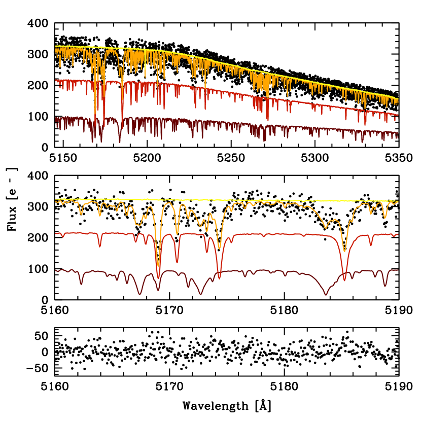
For faint stars, even if observed only a few days after new moon, the sky can contribute up to half of the observed spectra of faint M 4 targets. Otherwise the additional lines would lower the continuum level determined using only the stellar synthesis. Fortunately, our spectral range ($5140$Å $<\lambda<5360$Å) is free from atmospheric absorption lines, so no correction is required for this potential issue.

Figure 10: The $LSQ$ function for the same observations shown previously, before (red line) and after (black) sky subtraction. The blue line represents the gaussian fit to determine the RV of the star.

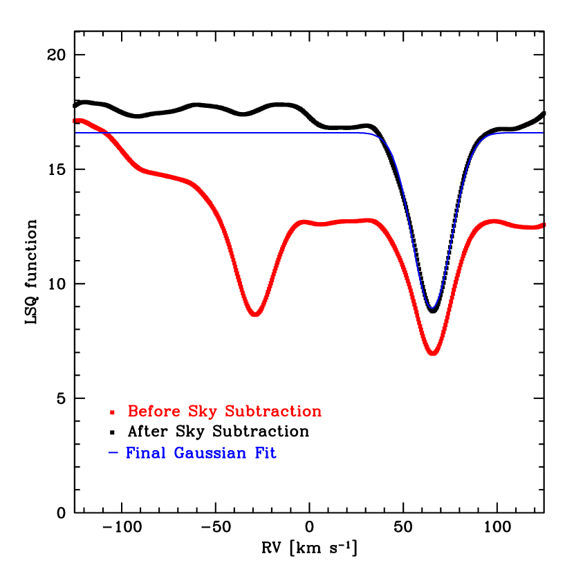
Fig. 10 shows the $LSQ$ function for this observation before and after the removal of the sky spectrum. The spectrum has been normalized using the continuum associated to the combined sky$+$synthesis in the first case, and the continuum associated to the synthesis alone in the second case after sky removal. The slope introduced by the contribution of the sky, which inevitably alters the shape of the curve associated to the star, is essentially gone after sky-subtraction from the observed spectrum. Finally, confidence in this approach for removing sky contamination and continuum normalization is increased by noting that stars with multi-epoch observations show lower internal dispersion in their RVs than can be obtained with other methods.

6 Results

After sky subtraction and normalization, the radial velocity is finally determined with a gaussian fit of the resulting $LSQ$ function, determined as described in 5.

Radial velocities shifts due to the intrinsic velocity of the star and the Earth motion are then applied to the stellar synthetic spectrum. Heliocentric and Barycentric corrections are determined using the FORTRAN subroutine by Stumpff (1980).

The error in the radial velocity associated with a single exposure is a function of the spectral type of the star, the characteristics of the instrument, the radial velocity determination technique and the SNR of the spectrum. Instead of trying to determine a formal velocity error of a single exposure, we determine an empirical error using the several radial velocity measurements available for each star.

The weighted mean velocity of a star $v_{r}$ is determined using Equation 5, where $r$ is the index of the star, $j$ is the index referring to individual exposures and $n$ is the total number of observations available for the given star.

$$\overline{v_{r}}=\frac{\Sigma_{j=1}^{n}w_{r,j}v_{r,j}}{\Sigma_{j=1}^{n}w_{r,j}}.$$ (5)

We use as weight $w_{r,j}$ the inverse of the minimum of the $LSQ$ function (Fig. 10) after normalizing it for the number of pixels used.

Following S09, the unbiased estimator for the population variance is determined with

$$(\sigma_{v_{r}})^{2}=\frac{\Sigma_{j=1}^{n}w_{r,j}}{(\Sigma_{j=1}^{n}w_{r,j})^{2}-\Sigma_{j=1}^{n}w_{r,j}^{2}}~{}\Sigma_{j=1}^{n}w_{r,j}(v_{r,j}-v_{r})^{2}.$$ (6)

It is interesting to compare the distribution of the radial velocity dispersion associated to each star before and after the SimCals correction for three different intervals in de-reddened V magnitude (Fig. 11). Going from the lower panel to the upper one, we can see how the correction for instrumental drifts in the radial velocity becomes increasingly more important for brighter stars, i. e. with higher SNR. This improvement is highlighted by the difference in the median values of the two distributions (vertical lines in the Figure). Although radial velocity measurements for faint stars are mostly dominated by photon noise, a small improvement in the $\sigma_{v_{r}}$ is still present.

Figure 11: Distribution of the radial velocity dispersion $\sigma_{v}$ associated to each star before (red lines) and after (black lines) the SimCals correction. Vertical lines mark the median values of the two distributions. Three ranges in de-reddened V magnitude are considered.

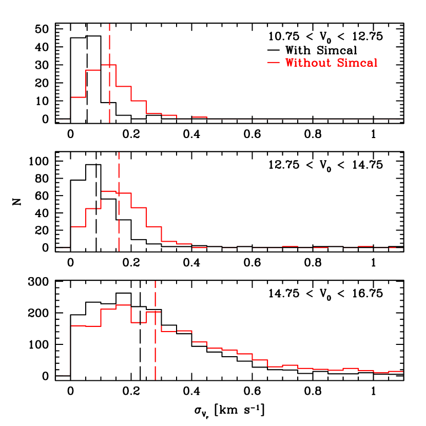
The average scatter $\langle\sigma_{v_{r}}\rangle^{bin}$ for a magnitude bin is computed as the $68.27^{\rm th}$ percentile of $\sigma_{v_{r}}$ distribution. This value is computed for several magnitude bins and the resulting values are interpolated to determine the estimated error in the radial velocity as a function of magnitude $\langle\sigma_{v_{r}}\rangle(V)$ (the subscript is omitted for the sake of brevity in the next sections). In the left-hand panel of Fig. 12 we show the computed $\langle\sigma_{v_{r}}\rangle$ values for our M 4 stars that have multi-epoch observations. In addition, we show the comparable trend that was derived by S09 (red thick line in Fig. 10 of their paper, blue line in Fig. 12). In the right-hand panel of this figure we show histograms of $\sigma_{v_{r}}$ in five magnitude bins. To ensure a fair comparison, we did not include the data acquired in 2009 in this analysis (see Section 2). At high SNR (i. e. $V_{0}<13$) the error is dominated by the instrumental stability, the goodness of the SimCals correction and the precision of the RV determination technique, for a total uncertainty of $\simeq 100$ m s^-1 ($<0.0018$ Å, or $<0.02$ pixel). We regard this as the practical precision limit in radial velocity that can be obtained from these GIRAFFE data.

Figure 12: The unbiased weighted radial velocity dispersion determined for stars with multi-epoch measurements. The estimated error on the radial velocity as a function of magnitude $\langle\sigma_{v_{r}}\rangle(V)$ from our analysis (red thick line), is compared with the one obtained by Sommariva et al. (2009) (blue line) using the same dataset. The histograms of the distribution for different ranges of magnitude are shown on the right panels, where the vertical lines follow the same convention defined in the left panel. Stars that satisfy the condition $\sigma_{v_{r}}>3\langle\sigma_{v_{r}}\rangle$ are considered binary candidates.

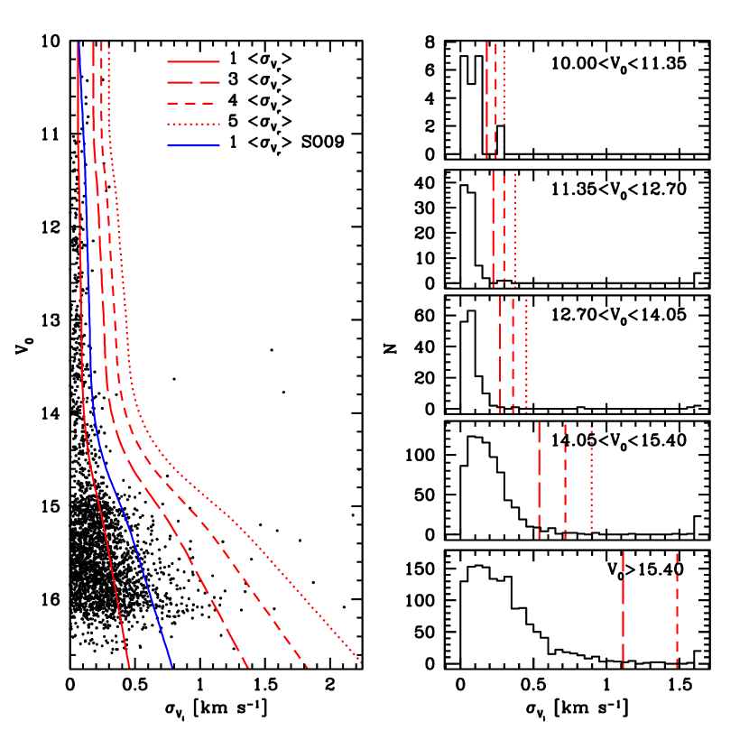
For brighter (RGB) M 4 stars the effect of the sky in RV determination is negligible even for observations obtained close to the full moon. For fainter stars with lower SNR data, the quality of the spectra becomes the main component in the precision of the RV determination. The combination of an improved wavelength calibration and careful determinations of radial velocities result in an increased precision of about a factor of two compared to the S09 results in the radial velocity determination of a single star.

Following S09, we consider stars with $\sigma_{v_{r}}>3\langle\sigma_{v_{r}}\rangle$ to be M 4 binary candidates. Using their same dataset, i. e., without data taken in 2009, we find 22 candidates out of 454 targets with $V_{0}<14.9$, and 55 candidates out of 2068 targets with $V_{0}>14.9$, for a total of 77 binary candidates. A total of 20 more candidates are found compared to the previous analyses by S09, using the same dataset and the same statistical approach. When the data from 2009 are included in the analysis 10 additional binary candidates with $V_{0}>14.9$ are found, with the total number of candidates growing to 87. Results are summarized in Table 3, while individual RVs are reported in table 4.

Table 3: Average radial velocities of the 2791 stars of the sample. Only a sample is given here, the full table will be available in the online version of the manuscript, together with a table comprising the binary candidates only.

$\alpha$ (J2000)	$\delta$ (J2000)	ID	$V$	$(B-V)$	$V_{0}$	$(B-V)_{0}$	No. Obs.	$v_{r}$	$\sigma_{v_{r}}$	$\langle\sigma_{v_{r}}\rangle$	$\sigma_{v_{r}}/\langle\sigma_{v_{r}}\rangle$
								km s-1	km s-1	km s-1	km s-1
245.838250	-26.513639	29622	16.329	0.970	14.974	0.615	2	70.553	0.115	0.221	0.521
245.892417	-26.504083	40918	14.505	1.139	13.146	0.771	2	70.963	0.023	0.088	0.266
245.913167	-26.483389	46022	15.016	1.103	13.649	0.742	3	63.619	0.084	0.094	0.891
245.941333	-26.560778	51878	12.935	1.282	11.570	0.930	10	67.314	0.266	0.069	3.834
245.897083	-26.537944	42121	12.944	1.245	11.566	0.873	10	79.513	6.666	0.069	96.145
…	…	…	..	…	…	…	…	…	…	…	…

Table 4: Individual radial velocities of the 2791 stars of the sample. Only a sample is given here, the full table will be available in the online version of the manuscript.

ID	MJD	j	GIRAFFE File	Fib	BERV	$v^{obs}_{r,j}$	$v_{r,j}$	fwhm	SNR	$(\chi^{2})^{-1}$
34087	52819.117744	1	GIRAF.2003-06-29T02:49:33.104	2	-13.951	83.002	69.051	9.971	7.25	105.998
34087	53982.999641	2	GIRAF.2006-09-04T23:59:28.940	22	-29.533	99.591	70.058	9.226	12.08	171.798
30327	52819.117744	1	GIRAF.2003-06-29T02:49:33.104	3	-13.957	86.523	72.566	9.048	8.61	134.988
30327	53947.065775	2	GIRAF.2006-07-31T01:34:42.930	5	-25.373	98.630	73.257	8.734	16.38	185.676
30327	53981.986284	3	GIRAF.2006-09-03T23:40:14.963	5	-29.544	102.366	72.822	9.420	12.66	161.065
…	…	…	…	…	…	…	…	…	…	…

Target stars have been carefully selected using multi-band photometry and proper motions, drastically reducing the chance of contamination by other stars. If present, contaminated spectra would have caused anomalous values in the FWHM or depth of the fitting function, which however have not been observed.

We did not attempt to determine the cluster binary fraction because the limited number of available epochs requires detailed completeness simulations, which are beyond the scope of our work, but it is likely that the true fraction in the outskirts of the cluster is substantially less than 0.1, in agreement with Milone et al. (2012) and Nascimbeni et al. (2014, Paper III). A future paper of the series will deal with the fraction and spatial distribution of binaries in M4̃ with a joint analysis of photometry, RV and proper motions.

6.1 Mean radial velocity and velocity dispersion

The average velocity of M 4 has been computed for four magnitude bins. Binary candidates are excluded from the sample, while we retain stars with only one RV measurement by assigning them $\sigma_{v_{i}}=\langle\sigma_{v_{r}}\rangle$ evaluated at their magnitude. Outliers in the CMD and obvious non-members (i. e. those stars with RV lower than 55 km s^-1 or higher than 87 km s^-1) are excluded as well, leading to a total of 2543 stars out of the 2771 of the initial sample. The weighted radial velocity mean for the cluster, the associated error, the dispersion of the distribution, and the number of stars for each magnitude bin are reported in Table 5 and displayed in Fig. 13. Errors on RV dispersions have been calculated as described in § 6.2 There is no significant trend in the cluster mean radial velocity with magnitude.

Table 5: Radial velocity means

N	$V_{0}$ range	$\langle v_{c}\rangle$	$\sigma_{\langle v_{c}\rangle}$	$\mu_{v_{c}}$	$\sigma_{\mu_{v_{c}}}$
		km s-1	km s-1	km s-1	km s-1
113	$10.10\leq V_{0}<12.8$	71.19	0.33	3.56	0.24
168	$12.80\leq V_{0}<14.15$	70.97	0.33	4.33	0.24
911	$14.15\leq V_{0}<15.50$	70.86	0.13	3.97	0.09
1351	$15.50\leq V_{0}<16.85$	71.26	0.11	3.94	0.08
totals:
2543	$10.2\leq V_{0}<17.0$	71.08	0.08	3.97	0.05

Figure 13: The weighted radial velocity mean of the cluster, the dispersion of the distribution and the number of stars for four magnitude bins, delimited with a grey line in the CMD. Candidate binary stars are denoted in red. There is no significant trend of the mean velocity of the cluster with magnitude.

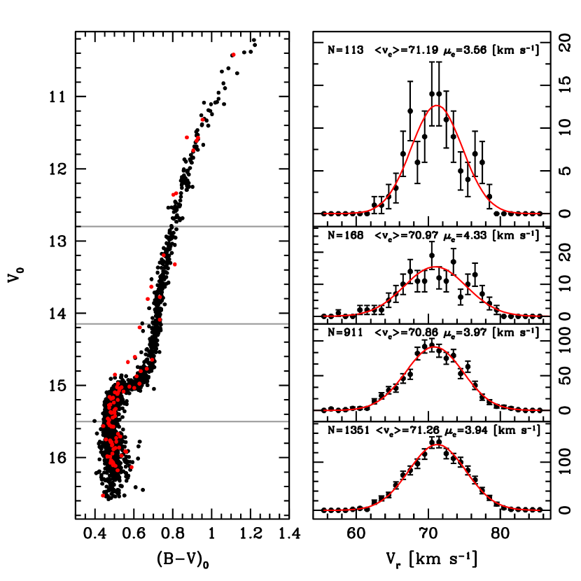
Our measured mean radial velocity for M 4 is $\langle v_{c}\rangle=71.08\pm 0.08$ km s^-1 with a cluster dispersion of $\mu_{v_{c}}=3.97\pm 0.05$ km s^-1. This value is in agreement with previous studies. P95 reported a radial velocity mean of $\langle v\rangle=70.9\pm 0.6$ km s^-1 using 200 giant stars. Côté & Fischer (1996) derived a value of $70.3\pm 0.7$ km s^-1 from the analysis 33 turn-off dwarf stars. Our analysis marginally agrees with the one performed by S09, which determined a mean radial velocity of $70.27\pm 0.19$ km s^-1 using our same dataset. The main differences with that study, as described in previous sections, are in the wavelength calibration and in their use of a numerical mask. Unfortunately no radial velocity standards are present in our dataset, so for the moment it is not possible to assess the origin of this small offset.

Before discussing the RV dispersion as a function of the distance from cluster center, note from the two upper-right panels in Fig. 13 that the RV distribution for RGB and SGB stars deviates from a simple gaussian distribution. To verify that these deviations do not affect the determination of the radial dispersion profile of the cluster, in Fig 14 we have plotted the RV distribution of RGB stars ($V_{0}<14.75$) for seven annuli of radial distance and for the full dataset (in the last panel on the right). The gaussian fit obtained using the full RGB sample is shown for comparison in all the panels, after properly rescaling for the total number of stars in each sample.

Figure 14: RV distribution of RGB stars ($V_{0}<14.75$) for seven radial annuli (as defined in the label of each panel) and for the whole dataset (last panel on the right side). The distribution obtained by including all the RGB stars, rescaled for the number of stars inside each annulus, is shown for comparison (blue curve).

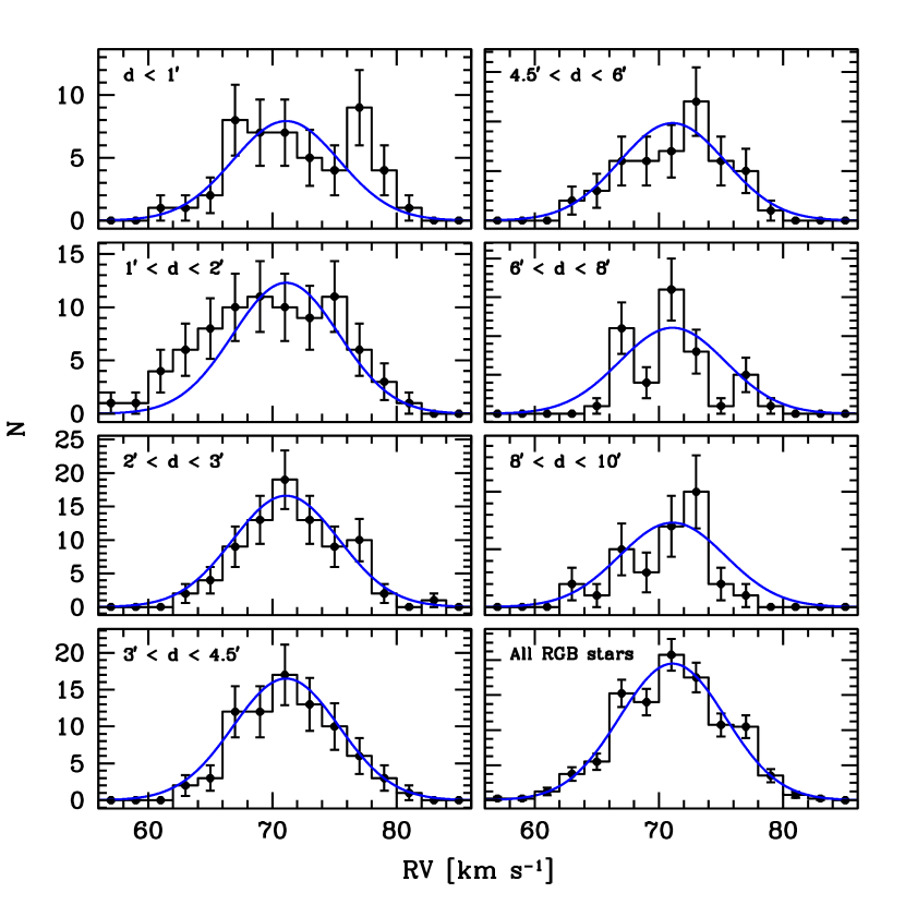
While the deviation from the normal distribution of each sample is not statistically significant, we have preferred to exclude the RGB and SGB stars from the following analysis since in our judgement they cannot provide a reliable picture of the kinematical status of the cluster. It is also likely that evolved stars have different kinematics with respect to MS stars as a consequence of mass segregation, thus supporting our choice of analysing the MS sample alone. The faintness of MS stars fortunately is not a limit in the determination of the kinematical properties of the cluster, thanks to the large size of the sample and our efforts in improving the RV precision.

6.2 Radial velocity dispersion

The dependence of the radial velocity dispersion with the distance from the cluster center is analysed by dividing our sample into 10 radial, circular annuli on the sky projected (tangent) plane and centered on $(\alpha,\delta)_{\rm J2000.0}$$=$$(\rm 16^{h}23^{m}35^{s}\!\!.22,$$\rm-26^{\circ}31^{\prime}32^{\prime\prime}\!\!.7)$ (Goldsbury et al., 2010). The weighted velocity dispersion in each bin is then calculated, as displayed in Fig. 15.

Figure 15: The radial velocity dispersion is plotted as a function of distance from the cluster center (black circles). Thanks to the larger sample and the improved RV precision, our data show that the velocity dispersion is steadily decreasing as a function of radius. This trend is suggested, but not statistically significant, by the data from Peterson, Rees & Cudworth (1995) (blue triangles)

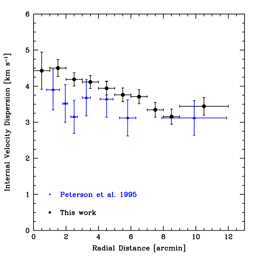
To take into account the broadening due to the observational uncertainty, for each bin the $68.27^{\rm th}$ percentile of the error distribution has been computed and the resulting value ($\simeq 0.3$ km s^-1) quadratically subtracted from the observed cluster dispersion $\mu_{v_{c}}$ in each bin. The error in the mean has been quadratically subtracted as well. We use the symbol $\mu_{\rm int}$ to distinguish the resulting value from the observed cluster dispersion. The vertical error for each bin has been determined following Peterson & Latham (1986) for a consistent comparison with P95 measurements. The square in the uncertainty in $\mu_{\rm int}^{2}$ has been computed as the sum of sampling error $\sigma_{N}^{2}=2/N\mu_{\rm int}^{4}$, where $N$ the number of stars in each bin, plus the error due to the uncertainty in a single measurements $\sigma_{\mu}^{2}=4/(N-1)\langle\sigma_{v_{r}}^{2}\rangle\sigma_{v_{c}}^{2}$. Following the propagation of uncertainty, the error in $\mu_{\rm int}$ is given by dividing the sum resulting from the previous step by $2\mu_{\rm int}$. Results are summarized in Table 6.

Table 6: Radial velocity dispersion as function of radial distance

$r$	$\sigma_{r}$	$\mu_{v_{c}}$	$\mu_{\rm int}$	$\sigma_{\mu_{\rm int}}$	No. Stars
arcmin	arcmin	km s-1	km s-1	km s-1
0.5	0.3	4.50	4.43	0.52	40
1.5	0.3	4.53	4.50	0.24	189
2.5	0.4	4.21	4.19	0.19	268
3.5	0.3	4.14	4.12	0.18	271
4.5	0.3	3.97	3.94	0.19	233
5.5	0.3	3.79	3.76	0.19	205
6.5	0.3	3.74	3.71	0.20	189
7.5	0.3	3.36	3.35	0.20	143
8.5	0.4	3.19	3.16	0.21	119
10.5	1.2	3.48	3.43	0.24	106

Thanks to the larger sample and the improved RV precision, our data show a steadily decreasing trend of the radial velocity dispersion as a function of radius. Our data are compatible with the one of P95, although in their case the trend is not statistically significant. This trend is still present with the same amplitude under different assumed statistical restrictions. These include: (a) considering only stars with at least three individual radial velocities; (b) applying a different $\sigma$-clipping on RV errors, i. e. $\sigma_{v_{r}}\leq 3\langle\sigma_{v_{r}}\rangle$ instead of $\sigma_{v_{r}}\leq 5\langle\sigma_{v_{r}}\rangle$; (c) selecting the stars in magnitude intervals. The radial distribution in P95 was determined using 182 members with a radial velocity precision of $\simeq 1$ km s^-1 for individual stars, while our sample comprises a larger number of stars (1763 MS members) and higher precision for a single star velocity determination (a few hundred m s^-1).

6.3 Rotation

Cluster rotation has been determined by following the same approach of Côté et al. (1995). Briefly, the cluster is halved by the position angle ${\rm PA}$, and the difference between the mean radial velocity of the two sides is computed, the error associated to each point being the sum in quadrature of the error on the mean of each side. The rotation curve as a function of the ${\rm PA}$ is then obtained by repeating the measurement for different values of the ${\rm PA}$. We adopted the same convention of Bellazzini et al. (2012; hereafter B12), i. e. the ${\rm PA}$ is increasing anti-clockwise from north (${\rm PA}=0^{\circ}$) to east (${\rm PA}=90^{\circ}$) in the plane of the sky, and the sine-function to fit the curve as $\Delta V_{r}=A_{\rm rot}\sin({\rm PA}+270-{\rm PA}_{0}$), where ${\rm PA}_{0}$ corresponds to the ${\rm PA}$ of the rotation axis and $A_{\rm rot}$ is the rotation amplitude projected on the plane of the sky and averaged over the range of radius of the sample. To better investigate the properties of the cluster, we have performed the analysis twice, by including all MS and SGB stars (which should share the same dynamical properties), and then by considering only only stars farther than $4^{\prime}$ from the cluster center, as previously done by P95. Binary candidates identified in Sec. 6 have been excluded from the analysis. The best-fit values are $A_{\rm rot}=0.51\pm 0.06$ km s^-1 and ${\rm PA}_{0}=127\pm 7^{\circ}$ for the whole sample, and $A_{\rm rot}=0.60\pm 0.07$ km s^-1 and ${\rm PA}_{0}=125\pm 7^{\circ}$ for the distance-selected one, thus being perfectly consistent. (Fig. 16). These values are obtained using a Monte Carlo method. Each data point is perturbed of a random value extracted from a normal distribution with the associated error as standard rotation, and the rotation curve is fitted. This procedure is then iterated 10.000 times to obtain a distribution of the two parameters and an estimate for their errors.

Figure 16: The difference between the mean velocities of the two halves of the cluster when divided by a line with varying PA, as a function of the PA itself. The best-fitting sine curve is shown. The analysis is performed on a sample including MS and SGB stars only (upper panel), and the same sample with only stars farther than 4^′ from the cluster center (lower panel).

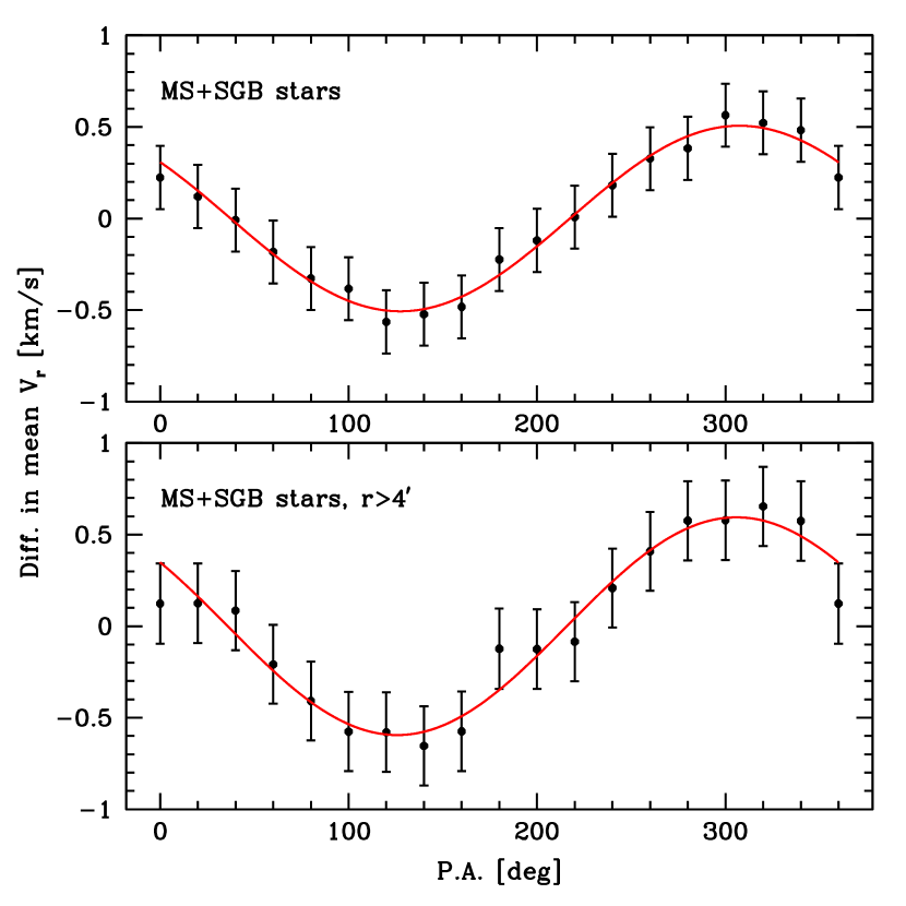
A common test to assess the statistical significance of the rotation signal is to perform a two-side Kolmogorov-Smirnov test on the cumulative distribution of RVs of stars that lie on opposite sides of the rotation axis (B12, Lardo et al. 2015). The presence of rotation induces a shift between the two distribution, see Fig. 17, hence the KS test quantify the probability to obtain the observed distribution under the null hypothesis that no rotation is present. We obtain $P_{\rm KS}=4.5\%$ and $P_{\rm KS}=0.4\%$ for the full sample and the distance-selected one respectively. The lower probability in the second case is expected, since we have removed from the sample the central region of the cluster, where the projected rotational velocity becomes negligible. For the RGB stars alone we obtain $P_{\rm KS}>20\%$, so we have not included the analysis in the text.

Figure 17: Comparison of the cumulative $v_{r}$ distribution of stars on the left (dashed lines) and on the right (continuous lines) side of the rotation axis of the cluster. The cumulative distributions along with the probability of null-hypothesis of the Kolmogorov-Smirnov test $P_{\rm KS}$ is shown for the whole MS$+$SGB sample (upper plot), and for MS$+$SGB stars farther than $4\arcsec$ from the cluster center. This result confirms the moderate rotation already observed in previous works.

Our results are consistent with the previous claim of moderate rotation for this cluster of P95. We found a rotation amplitude several times smaller than the value of $A_{\rm rot}=1.8\pm 0.2$ km s^-1of Lane et al. (2010), although they quote half of this value as the rotation velocity.

7 Conclusions

We have presented a new approach for the determination of accurate wavelength dispersion solutions for not-stabilized instruments. We have developed an algorithm for improved corrections for radial velocity shifts using simultaneous calibration fibres. Several precautions have to be taken when dealing with low SNR spectra covering a short wavelength range and strong absorption features, in particular during sky spectrum subtraction and continuum normalization. Together with a careful choice of the radial velocity technique that better suites the characteristics of our spectra, we have been able to significantly increase the precision of the radial velocities with respect to existing tools. Algorithms have been optimized to require only a minimal user interaction.

The code we have developed is lacking the necessary documentation to be user-friendly at present. While we do not exclude a general release in the next future, we have decided to not make it public yet. Instead, we provide a very detailed description of each step of our methodology with the hope that large consortium dedicated to data reduction, such as the Gaia-ESO or ESO itself, can implement and eventually improve it for other GIRAFFE settings as well other instruments.

Our new radial velocity procedures have been tested on a large dataset for globular cluster M 4 with extant state-of-the-art radial velocity measurements in the literature, in order to assess the improvement in velocity precision. A total of 7250 individual spectra for 2771 stars, gathered with the GIRAFFE spectrograph at VLT during a multi-epoch campaign, have been analysed, for a total of 2543 stars after removing non-members and candidate binaries. The derived cluster radial velocity is $\langle v\rangle=71.08\pm 0.08$ km s^-1, in agreement with previous measurements in literature but with an offset of $\Delta v=0.81$ km s^-1 with the previous value derived using the same dataset (probably due to the different radial velocity determination technique). We found a total of 87 binary candidates, 22 giants and 65 sub-giants and dwarfs, which is a significative increase of the number found by previous analyses.

From our data we have measured a rotational amplitude of $\simeq 0.5$km s^-1, providing a statistical confirmation of the negligible rotation of this cluster. An average radial velocity dispersion of $4.5$ km s^-1 within 2$\arcmin$ from the center of cluster and steadily decreasing outward has been found, in contrast with the nearly constant value of $3.5$ km s^-1 from P95. Our new determination is going in the same direction of recent simulations from Heggie (2014), where a N-body simulation of the cluster results in a RV dispersion steadily, and it will further improve the dynamical modeling of M4. Ultimately, the combination of these data with the unprecedented precision of the proper-motions that will be delivered by the HST Large Program described in Paper I and following will provide a deeper insight into the three-dimensional dynamics of the cluster and a new, more accurate determination of its geometrical distance, among other things.

References

- Anderson et al. (2006) Anderson J., Bedin R. R., Piotto G., Yadav R. S., Bellini A., 2006, A&A, 454, 1029
- Anderson & King (2000) Anderson J., King I. R., 2000, PASP, 112, 1360
- Baranne et al. (1996) Baranne A. et al., 1996, Astron Astrophys Sup, 119, 373
- Baumgardt et al. (2009) Baumgardt H., Côté P., Hilker M., Rejkuba M., Mieske S., Djorgovski S. G., Stetson P., 2009, MNRAS, 396, 2051
- Bedin et al. (2013) Bedin L. R. et al., 2013, Astronomische Nachrichten, 334, 1062
- Bellazzini et al. (2012) Bellazzini M., Bragaglia A., Carretta E., Gratton R., Lucatello S., Catanzaro G., Leone F., 2012, A&A, 538, 18
- Blecha et al. (2000) Blecha A., Cayatte V., North P., Royer F., Simond G., 2000, Proc. SPIE Vol. 4008, 4008, 467
- Bristow et al. (2010) Bristow P., Vernet J., Kerber F., Moehler S., Modigliani A., 2010, in Society of Photo-Optical Instrumentation Engineers (SPIE) Conference Series, Vol. 7735, Society of Photo-Optical Instrumentation Engineers (SPIE) Conference Series, p. 7
- Brown & Wallerstein (1992) Brown J. A., Wallerstein G., 1992, AJ, 104, 1818
- Casagrande et al. (2010) Casagrande L., Ramírez I., Meléndez J., Bessell M., Asplund M., 2010, A&A, 512, 54
- Castelli & Kurucz (2004) Castelli F., Kurucz R. L., 2004, arXiv, astro-ph
- Côté & Fischer (1996) Côté P., Fischer P., 1996, Astronomical Journal v.112, 112, 565
- Côté et al. (1995) Côté P., Welch D. L., Fischer P., Gebhardt K., 1995, Astrophysical Journal v.454, 454, 788
- D’Antona et al. (2009) D’Antona F., Stetson P. B., Ventura P., Milone A. P., Piotto G., Caloi V., 2009, Monthly Notices of the Royal Astronomical Society: Letters, L319
- de Boor (1977) de Boor C., 1977, Journal of Numerical Analysis, 14, 441
- Dinescu et al. (1999) Dinescu D. I., van Altena W. F., Girard T. M., López C. E., 1999, AJ, 117, 277
- D’Orazi et al. (2013) D’Orazi V., Campbell S. W., Lugaro M., Lattanzio J. C., Pignatari M., Carretta E., 2013, MNRAS, 433, 366
- Enard (1982) Enard D., 1982, Society of Photo-Optical Instrumentation Engineers (SPIE) Conference Series, 331, 232
- Feldmeier et al. (2013) Feldmeier A. et al., 2013, A&A, 554, A63
- Goldsbury et al. (2010) Goldsbury R., Richer H. B., Anderson J., Dotter A., Sarajedini A., Woodley K., 2010, AJ, 140, 1830
- Heggie (2014) Heggie D. C., 2014, MNRAS, 445, 3435
- Heggie & Giersz (2008) Heggie D. C., Giersz M., 2008, Monthly Notice of the Royal Astronomical Society, 389, 1858
- Hendricks et al. (2012) Hendricks B., Stetson P. B., Vandenberg D. A., Dall’Ora M., 2012, AJ, 144, 25
- Horne (1986) Horne K., 1986, PASP, 98, 609
- Ibata et al. (2011) Ibata R., Sollima A., Nipoti C., Bellazzini M., Chapman S. C., Dalessandro E., 2011, ApJ, 738, 186
- Ivans et al. (1999) Ivans I. I., Sneden C., Kraft R. P., Suntzeff N. B., Smith V. V., Langer G. E., Fulbright J. P., 1999, AJ, 118, 1273
- Kaluzny et al. (2013) Kaluzny J. et al., 2013, AJ, 145, 43
- Kirby, Guhathakurta & Sneden (2008) Kirby E., Guhathakurta P., Sneden C., 2008, ApJ, 682, 1217
- Kurtz & Mink (1998) Kurtz M. J., Mink D. J., 1998, PASP, 110, 934
- Kurucz (1992) Kurucz R. L., 1992, in The Stellar Populations of Galaxies: Proceedings of the 149th Symposium of the International Astronomical Union, p. 225
- Kurucz et al. (1984) Kurucz R. L., Furenlid I., Brault J., Testerman L., 1984, Solar flux atlas from 296 to 1300 nm. National Solar Observatory
- Lane et al. (2010) Lane R. R. et al., 2010, Monthly Notice of the Royal Astronomical Society, 406, 2732
- Lardo et al. (2015) Lardo C. et al., 2015, A&A, 573, A115
- Libralato et al. (2014) Libralato M., Bellini A., Bedin L. R., Piotto G., Platais I., Kissler-Patig M., Milone A. P., 2014, A&A, 563, A80
- Lovis & Pepe (2007) Lovis C., Pepe F., 2007, A&A, 468, 1115
- Lützgendorf et al. (2013) Lützgendorf N. et al., 2013, A&A, 552, A49
- Malavolta et al. (2014) Malavolta L., Sneden C., Piotto G., Milone A. P., Bedin R. R., Nascimbeni V., 2014, AJ, 147, 25
- Marino et al. (2008) Marino A. F., Villanova S., Piotto G., Milone A. P., Momany Y., Bedin R. R., Medling A. M., 2008, A&A, 490, 625
- Milone et al. (2014) Milone A. P. et al., 2014, MNRAS, 439, 1588
- Milone et al. (2012) Milone A. P. et al., 2012, A&A, 540, 16
- Milone et al. (2006) Milone A. P., Villanova S., Bedin R. R., Piotto G., Carraro G., Anderson J., King I. R., Zaggia S., 2006, A&A, 456, 517
- Monelli et al. (2013) Monelli M. et al., 2013, MNRAS, 431, 2126
- Murphy et al. (2007) Murphy M. T., Tzanavaris P., Webb J. K., Lovis C., 2007, Monthly Notice of the Royal Astronomical Society, 378, 221
- Nardiello et al. (2015) Nardiello D., Milone A. P., Piotto G., Marino A. F., Bellini A., Cassisi S., 2015, A&A, 573, A70
- Nascimbeni et al. (2014) Nascimbeni V. et al., 2014, MNRAS, 442, 2381
- Pasquini et al. (2000) Pasquini L. et al., 2000, Society of Photo-Optical Instrumentation Engineers (SPIE) Conference Series, 4008, 129
- Pepe et al. (2002) Pepe F., Mayor M., Galland F., Naef D., Queloz D., Santos N. C., Udry S., Burnet M., 2002, A&A, 388, 632
- Pepe et al. (2004) Pepe F. et al., 2004, A&A, 423, 385
- Peterson & Latham (1986) Peterson R. C., Latham D. W., 1986, Astrophysical Journal, 305, 645
- Peterson, Rees & Cudworth (1995) Peterson R. C., Rees R. F., Cudworth K. M., 1995, ApJ, 443, 124
- Piotto et al. (2015) Piotto G. et al., 2015, AJ, 149, 91
- Ramírez & Meléndez (2005) Ramírez I., Meléndez J., 2005, ApJ, 626, 465
- Royer et al. (2002) Royer F., Blecha A., North P., Simond G., Baratchart S., Cayatte V., Chemin L., Palsa R., 2002, Astronomical Data Analysis II. Edited by Starck, 4847, 184
- Smith & Briley (2005) Smith G. H., Briley M. M., 2005, PASP, 117, 895
- Sneden (1973) Sneden C., 1973, Astrophysical Journal, 184, 839
- Sommariva et al. (2009) Sommariva V., Piotto G., Rejkuba M., Bedin R. R., Heggie D. C., Mathieu R. D., Villanova S., 2009, A&A, 493, 947
- Sousa et al. (2007) Sousa S. G., Santos N. C., Israelian G., Mayor M., Monteiro M. J. P. F. G., 2007, A&A, 469, 783
- Stumpff (1980) Stumpff P., 1980, Astron Astrophys Sup, 41, 1
- Tonry & Davis (1979) Tonry J., Davis M., 1979, Astronomical Journal, 84, 1511
- Yong et al. (2008) Yong D., Karakas A. I., Lambert D. L., Chieffi A., Limongi M., 2008, ApJ, 689, 1031