On the IMF in a triggered star formation context^†

Abstract

The origin of the stellar initial mass function (IMF) is a fundamental issue in the theory of star formation. It is generally fitted with a composite power-law. Some clues on the progenitors can be found in dense starless cores which have a core mass function (CMF) with similar shape. In the low-mass end, these mass functions increase with mass, albeit the sample may be somewhat incomplete, whereas they decrease with mass in the high-mass end. There is an offset in the turn-over mass between the two mass distributions. The stellar mass for the IMF peak is lower than the corresponding core mass for the CMF peak in the Pipe nebula by about a factor of three. Smaller offsets are found between the IMF and the CMFs in other nebulae. We suggest that the offset is likely to be induced during a star-burst episode of global star formation which is triggered by the formation of a few O/B stars in the multi-phase media, which is naturally emerged by the onset of a thermal instability in the cloud-core formation process. We consider the scenario that the ignition of a few massive stars photoionizes the warm medium between the cores, increases the external pressure, reduces their Bonnor-Ebert mass and triggers the collapse of some previously stable cores. We quantitatively reproduce the IMF in the low-mass end with the assumption of additional rotational fragmentation.

1. Introduction

Recent infrared measurements of dust extinction, as well as CO and ${\rm NH_{3}}$ maps of the filaments in molecular clouds reveal a population of embedded cores mostly confined by the global external pressure from the inter-core gas. These cores are closely associated with the progenitors of young stellar objects. In such filaments there are gravitationally bound cores (or pre-stellar cores), and embedded protostars (André et al., 2010). But, in the Pipe nebula nearly all the cores are starless (Lada et al., 2008). Only the most massive cores in Pipe are gravitationally bound and might collapse. The shape of the CMF of these dense cores (Lada et al., 2008) appears to be qualitatively similar to the broken power-law of the stellar IMF (Kroupa, 2002; Weidner et al., 2011). An in-depth analysis of their structure and evolution may be useful for the construction of a star formation theory.

One noticeable difference between the CMF and the IMF is an offset between the two distributions. The ratio of the characteristic mass of the IMF over the characteristic mass of the CMF is generally smaller than unity. This ratio ranges from $\sim 1:3$ in the Pipe nebula (Rathborne et al., 2009) to $>1:2$ in the Orion (Nutter & Ward-Thompson, 2007) and Aquila nebulae (Könyves et al., 2010). Rathborne et al. (2009) proposed that this offset is due to a direct one-to-one mapping from the cores to the stars with sufficient amount of mass loss during the star formation process. It is hard to explain in this scenario how the low-mass stars are produced by the originally stable low-mass cores.

Many studies modeling the origin of IMF highlight factors such as the accretion rate of protostars, turbulent fragmentation and accretion of cores (see e.g., Bonnell & Bate, 2006; Clark et al., 2008; Anathpindika, 2011). In the meantime, constraints such as the small age spread of stars in young clusters are inconsistent in these models.

We propose a scenario to explain the transition from the CMF to the IMF as well as a synchronized star formation, triggered by a few first formed O/B stars in the nebula. Many authors (e.g., Strömgren, 1939; Spitzer, 1978) studied the effects of UV radiation from massive stars onto the surrounding regions. The UV radiation generates a hot ionized region (Strömgren sphere), increasing the ambient pressure. Consequently, an isothermal shock is driven through the nebula. Influenced by the Strömgren sphere, denser sub-structures are rapidly enhanced and most of the pre-existing pressure confined cores are compressed (e.g., Gritschneder et al., 2009). The ionization timescale is generally short compared to the hydrodynamical timescales, such that the increase in the background pressure and temperature can be considered instant in most cases.

In this work, we develop a quantitative understanding of the consequences of this sudden change in the ambient pressure and temperature in the context of the transition from the CMF to the IMF. A direct result is the reduction of the critical Bonnor-Ebert mass (Ebert, 1955; Bonnor, 1956), making previous unbound cores gravitationally unstable. Therefore, the whole region experiences a rapid star burst, synchronizing star formation. The shifted Bonnor-Ebert mass also naturally leads to the transition from the CMF distribution to the IMF distribution.

We base our calculations on a Pipe-like cloud, with a starless CMF as the starting point of the evolution. We investigated the formation of a starless CMF in our previous work (Huang et al. 2013, hereafter H13). In H13, we suggest that, prior to the onset of global star formation, the cores and the inter-core gas are two separate phases in pressure equilibrium, which possibly result from thermal instability (Lin & Murray, 2000). The dynamics of coagulation (Murray & Lin, 1996) and ablation (Murray et al., 1993) dominate the evolution of the system and the star formation timescale is prolonged by the turbulent pressure or magnetic pressure inside the cloud (Lazarian & Vishniac, 1999).

In this paper, we consider the consequences of the ignition of the first massive stars in a starless nebula. In §2, we suggest that the photoionization of the inter-cloud gas leads to a decrease in the critical Bonnor-Ebert mass and triggers a global burst of star formation. We use this reduced critical mass and the starless CMF from the Pipe to obtain the transition to a stellar IMF in §3. We assume different star formation statistics, showing that uncertainties such as binary mass ratio distribution do not affect the IMF shape in a certain parameter range. The discussion and conclusions are presented in §4.

2. Triggered star formation

After the formation of the first massive stars, their stellar luminosity has a significant influence on the subsequent evolution of the surrounding media. In the presence of a strong UV flux from nearby O/B stars, the diffuse neutral medium, originally at 100 K, hereafter referred to as the warm medium, would be ionized and heated up, while the dense molecular region, originally at 10 K, hereafter referred to as the cold medium, would still be mostly shielded. The resulting increase in the external pressure leads to a reduction in the Bonnor-Ebert mass of the cold cores and a decrease in the star formation timescale.

2.1. The ionization of the warm medium

The ionizing photons from the native stars create Strömgren spheres in the surrounding warm medium. For a typical O/B star with an effective UV photon ($E_{\gamma}>13.6\,{\rm eV}$) emission rate of $Q_{0}\sim 10^{48\sim 49}\,{\rm s^{-1}}$, the Strömgren radius $R_{S}$ is determined by

$$Q_{0}\sim\frac{4\pi}{3}\,R_{S}^{3}\,\alpha_{B}\,n_{\rm warm}^{2},$$ (1)

where $\alpha_{B}=2.6\times 10^{-13}\,T_{4}^{0.833-0.034\log{T_{4}}}\,{\rm cm^{3}s^{-1}}$ is the recombination coefficient (Draine, 2011). We define $T_{4}$ as the temperature of the warm medium in units of $10^{4}$ K, $Q_{\rm 0,49}$ as the number of UV photons in units of $10^{49}\,{\rm s}^{-1}$, and $n_{\rm warm,2}$ as the warm medium hydrogen number density in units of $10^{2}\,{\rm cm^{-3}}$. Within $R_{S}\sim 3\,{\rm pc}\,Q_{\rm 0,49}^{\frac{1}{3}}\,n_{\rm warm,2}^{-\frac{2}{3}}$ of the ionizing sources, the warm medium is nearly fully ionized, with $T_{\rm warm}\sim 10^{4}\,{\rm K}$. This new temperature corresponds to an increase by a factor of 10$\sim$100.

More realistic calculations of equilibrium temperature have been performed with version 08.00 of CLOUDY (last described by Ferland et al. 1998). The effective temperature of the central star is taken to be 34,700 K with a surface luminosity of log$(L/L_{\odot})=5.59$. This is a typical value for a main sequence star with a mass of $40M_{\sun}$, produced with the Cambridge stellar evolution code STARS (Eggleton, 1971). Assuming a blackbody, the star emits $31\%$ of its power in hydrogen ionization photons, corresponding to $Q_{0,49}\sim 1$.

We assume a solar metallicity for the gas and a standard dust composition. We use a constant hydrogen density of $n_{\rm H}=774\,{\rm cm^{-3}}$ to simulate the warm medium in Pipe nebula, to be consistent with the values in Gritschneder & Lin (2012).

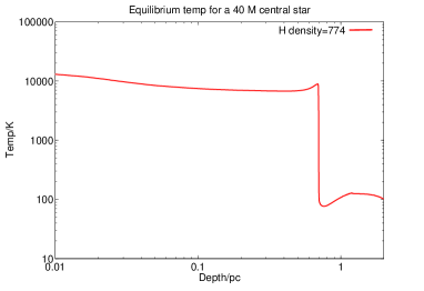
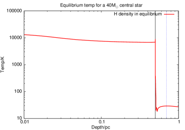
The results show that there is a sharp temperature dropoff from several thousand degrees to several hundred degrees at a particular depth of the cloud. The solid line in Figure 1 shows the temperature of the warm medium versus the distance from the star. This indicates the Strömgren radius is $0.7\,{\rm pc}$ and the temperature inside the ionized sphere is around $9000\,{\rm K}$. Given the typical size of a nebula, which is usually a few pc, only a few massive stars are needed to ionize most of the inter-core media, leading to a much higher exterior pressure.

2.2. Heating of the cold cores

The ionizing UV flux can also penetrate into dense cores. We first consider the heating from the radiation which balances the cooling from recombination.

We denote $R_{\rm ion}$ to be the distance from an O/B star at which a typical cold core is heated by the external radiation to 100 K. By neglecting the loss of ionizing photons from the star through the warm medium, we estimate $R_{\rm ion}$ from:

$$\frac{R_{\rm ion}}{0.7\,{\rm pc}}\sim(\frac{Q}{10^{49}\,{\rm s^{-1}}})^{\frac{1}{2}}\,(\frac{r_{c}}{0.1\,{\rm pc}})^{-\frac{1}{2}}\,(\frac{n_{c}}{10^{4}\,\rm{cm^{-3}}})^{-1}\\ \,(\frac{T_{c}}{100\,{\rm K}})^{-0.5},$$ (2)

where

$$Q_{0}\,\frac{\pi\,r_{c}^{2}}{4\pi\,R_{\rm ion}^{2}}\sim\frac{4\pi}{3}\,r_{c}^{3}\,\alpha_{\rm B}\,n_{\rm cold}^{2},$$ (3)

with $\alpha_{B}$ here is the same as in section 2.1.

More realistically, we compute the ionization in the cold core with CLOUDY, using the same setup as in §2.1, but this time with an initial hydrogen density $n_{\rm H}=774\,{\rm cm^{-3}}$ in the range of $0\sim 0.5\,{\rm pc}$, while $n_{\rm H}=7300\,{\rm cm^{-3}}$ from $0.5\,{\rm pc}$ to faraway, corresponding to the cold medium placed $0.5\,{\rm pc}$ from the central star, and the warm medium filling the space in between. Then instead of keeping constant density, we keep the two media in pressure equilibrium, as the central star illuminates its surroundings. In this case, the density of the cold medium is enhanced rapidly, due to the sudden increase of warm medium temperature and pressure. After the attenuation of the warm medium, the typical photon penetration depth inside the cold medium is only about $0.02\,{\rm pc}$. This is much smaller than the typical core radius $r_{c}\approx 0.1\,{\rm pc}$. Therefore, only cores very near the massive star or very small cores are subjected to this effect. The temperature inside the cores further away is limited by the cooling process to be around 15–20 K, which is two times higher than before the ignition of the UV flux (see Figure 1, for ${\rm depth}>0.5\,{\rm pc}$).

In addition, we also investigate the classical evaporation of cores due to the high temperature environment. Using the formula for the evaporation rate of clouds embedded in a $10^{4}$ K gas (Graham & Langer, 1973; Cowie & McKee, 1977; McKee & Cowie, 1977), with the limitations that the background gas is either fully ionized or neutral,

$$\dot{m}=\frac{16\pi\mu\kappa\,r_{c}}{25\,k}=\begin{cases}1.3\times 10^{15}\,T^{1/2}\,r_{\rm c,pc}\,{\rm g}\,{\rm s^{-1}}\,,&{\kappa=\kappa_{\rm n}}\cr 2.75\times 10^{4}\,T^{5/2}\,r_{\rm c,pc}\,{\rm g}\,{\rm s^{-1}}\,,&{\kappa=\kappa_{c}}\end{cases}$$ (4)

Here, $T$ is the environment temperature, $k$ is the Boltzmann’s constant, $r_{\rm c,pc}$ is the radius of the core in units of pc, $\kappa_{\rm n}$ is the neutral conductivity, $\kappa_{c}$ is the classical conductivity for a fully ionized gas . For a typical core with mass $m_{\rm c}$, the evaporation timescale therefore is $\tau_{\rm evap,n}=m_{\rm c}(\dot{m})^{-1}=8\times 10^{5}\,r_{\rm c,pc}^{2}\,{\rm Myr}$ in the neutral case and $\tau_{\rm evap,i}=4\times 10^{8}\,r_{\rm c,pc}^{2}\,{\rm Myr}$ in the fully ionized case. Based on these calculations, the classical evaporation only affects cores with radius as small as $0.01\,{\rm pc}$.

We conclude from the above calculation that the evaporation effect is negligible. This is understandable as both the recombination timescale and cooling timescale inside the cold medium are much shorter than these timescales inside the warm gas due to their density contrast. Therefore, the ionization fraction and temperature of the cold medium can be maintained at low levels. We do not include the change of the IMF due to the evaporation in the calculation below.

Figure 1.— Resulting temperature profiles in the surrounding of a 40 $M_{\sun}$ star for different gas profiles. (a) The red line displays the temperature profile in a medium with constant density $n_{0}=774\,{\rm cm^{-3}}$. The transition from ionized to un-ionized medium happens at $0.7\,{\rm pc}$ (the Strömgen radius). (b) This setup represents a cold core at a distance of $0.6\,{\rm pc}$ from the central star. The initial density profile is set to $n_{0}=774\,{\rm cm^{-3}}$ (inter-core medium) inside $0.5\,{\rm pc}$ and $n_{0}=7300\,{\rm cm^{-3}}$ (core medium) beyond $0.5\,{\rm pc}$. The solid vertical line indicates the inner side boundary of the core, i.e. the location of the density jump. The dashed vertical line indicates the extent of the core from the solid vertical line. For computational simplicity, we do not calculate the region behind the core, as the focus of this work lies on the penetration depth at the front side.

2.3. Change in Bonnor-Ebert mass and star formation timescale

The star formation timescale in general can be as long as $100~{}{\rm Myr}$ (Ostriker, 2011). However, the collapse process is speeded up considerably by the compression of the dense cores due to the UV feedback (Gritschneder et al., 2009). More importantly, the enhancement of the external pressure reduces the Bonnor-Ebert mass and induces the formation of low-mass stars.

The Bonnor-Ebert mass of a cold core can be expressed as $m_{\rm BE}\propto P_{\rm ext}^{-0.5}T_{\rm int}^{2}$ where $P_{\rm ext}$ is the external pressure (see also equation(4) in Lada et al. 2008). Prior to the formation of a massive star, the temperature of the warm medium is $T_{\rm ext}\sim 100~{}{\rm K}$, and the cores’ temperature is $T_{\rm int}\sim 10~{}{\rm K}$. In a pressure equilibrium, the density contrast between the cores and medium is $\sim 10$. The influx of the UV photons from an emerging massive star ionizes the tenuous warm medium within a pc from the star and raises the medium’s temperature to $T_{\rm ext}\sim 9000~{}{\rm K}$. In contrast, the temperature within the cores remains at $T_{\rm int}\sim 20~{}{\rm K}$ (see Fig 1).

The ionization front propagates through the warm medium more rapidly than the sound speed. Consequently, the increase in $T_{\rm ext}$ leads to an increase in $P_{\rm ext}$ by a similar factor before the medium’s density can readjust to a new pressure equilibrium. Due to the combined effect of the temperature and pressure increase in both the warm medium and the cold medium, the Bonnor-Ebert mass decreases by a factor of 2.38, shifting from around $2~{}M_{\odot}$ (Lada et al., 2008) to $0.84~{}M_{\odot}$ in our model.

Due to this sudden increase of the external pressure, global, coordinated star formation is induced, leading to a star burst. Several factors may introduce some dispersions in the value of the modified $m_{\rm BE}$. For example, the flux of ionizing photons emitted by the first O/B star would be reduced by an order of magnitude if its mass is halved (the one we have considered in Figure 1 is $40~{}M_{\odot}$). Nevertheless, the final temperature of the ionized region and the core only change slightly. The Bonnor-Ebert mass associated with slightly lower $T_{\rm ext}$ ($8500~{}{\rm K}$) and $T_{\rm int}$ ($15~{}{\rm K}$) would reduce $m_{\rm BE}$ to $0.47~{}M_{\odot}$. In this case, the Strömgren sphere around the star will be much smaller, which would slow down the global star formation process and extend the age spread in this nebula. If the global star formation timescale is comparable or longer than the timescale of core coagulation, the dynamics of cores may affect the IMF further. Here, we neglect this effect on the age spread and the effect from the evolution of cores. Once a core becomes gravitationally unstable, it collapses on a free fall timescale.

$$t_{\rm sf}\sim t_{\rm ff}=\sqrt{\frac{r_{\rm c}^{3}}{G\,m_{\rm c}}}\sim 0.3\,{\rm Myr}(\frac{r_{\rm c}}{0.1\,\rm pc})^{3/2}(\frac{m_{\rm c}}{2\,M_{\sun}})^{-1/2}.$$ (5)

This timescale is much shorter than that associated with the dynamical evolution of the dense cores prior to the formation of the first massive stars, which is about $5~{}{\rm Myr}$ from H13. After the external medium is ionized by the first massive stars, the compression of the cores reduces the cross section and enhances the density contrast between the core and the external medium.This increases both the coagulation and the fragmentation timescales. Therefore, the further dynamical evolution of the CMF can be neglected.

Figure 2.— CMFs and IMFs generated in our model under different assumptions. (a) The CMF obtained from H13 (solid black line) is adopted as the initial condition for our calculations. Grey line shows the observed CMF in the Pipe from Rathborne et al. (2009). For comparison, the Chabrier IMF (Chabrier, 2003), shifted to the low mass end by a factor of 3, is shown as the dashed blue line. (b) Grey curves are displaying the stellar IMFs for single stars with different retention factors $\eta_{\rm sf}(m_{c})$. Any core evolution through coagulation or fragmentation is neglected. (c) The black solid line is showing the generated total IMF if all the cores undergo binary fragmentation with $\beta=0.2$ (see Equation 8) and $\eta_{\rm sf}(m_{c})=0.3$. (d)The black solid line is showing the total IMF, assuming $100\%$ binary star formation. The secondary stellar masses follow a power-law distribution with index $\alpha=1.5$ (see Equation 9). We show both the Chabrier IMF (blue dashed curve) and the Kroupa IMF (Kroupa, 2002)(grey dash-dotted lines) as a comparison. The modeled IMF is fitted with a broken power-law (red dash-dotted lines).

Figure 3.— Analytical results for f(q), i.e., the probability distribution function (PDF) of observed mass ratios ($\textit{q}=m_{\rm sec}/m_{\rm prim}$) in binary systems. The conditional distribution of mass ratio given the progenitor core mass is assumed to be a uniform distribution in ($\textit{q}_{\rm min}$,1) regardless of $m_{\rm core}$ (see Eq.13). For the CMF prescription $dn/dm=m^{-\alpha}$, the blue line corresponds to $\alpha=1.3$ and the red line corresponds to $\alpha=2.35$. The total accumulated probability is renormalized to 1 and $\textit{q}_{\rm min}=0.05$. The dashed line is the best fit power-law ($f(\textit{q})\propto\textit{q}^{-0.4}$) to the observations from Kouwenhoven et al. (2007).

3. From the CMF to the IMF

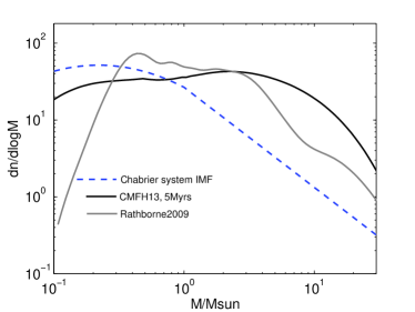
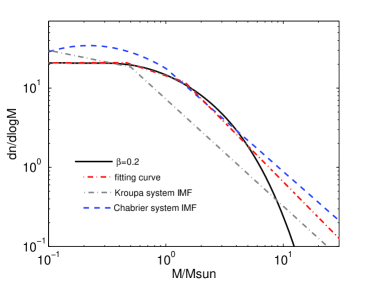
The initial stellar mass function is determined by the induced collapse of the dense cores with a preset CMF. The calculations presented here follow our previous work on the CMF (H13). In the previous paper, we discussed the evolution of the dense core mass distribution with a modified coagulation equation. The CMF acquires a stable shape which resembles a typical observed CMF after several million years of evolution time. During this stage prior to the triggered star formation we discuss here, a typical star formation timescale is around $100~{}{\rm Myr}$, which keeps the starless nature of the system. Figure 2 shows the pre-stellar core mass distribution compared with the Chabrier System IMF (Chabrier, 2003) and recent observations (Rathborne et al., 2009). The intermediate mass range of the CMF ($0.3\textendash 0.5$ $M_{\odot}$) can be also parameterized with similar two power-law slopes as the Kroupa IMF, only shifted to a higher mass range by a factor of about $3$ (Lada et al., 2008). We note that both the observed CMF and modeled CMF have a slightly steeper slope than the IMF at the high mass end. However, the uncertainty is also higher in those bins due to small number statistics. We now take the modeled CMF (H13) as the initial condition and assume the global star formation is triggered simultaneously. During a time step $\delta t$, the number of stars in the mass range $m\sim m+dm$ increases by

$$\frac{\Delta{n^{*}(m^{*})}}{\Delta{t}}=\\ \int_{m_{\rm min}}^{m_{\rm max}}m_{c}n(m_{c})\eta_{\rm sf}\gamma_{\rm sf}\\ \frac{P(m_{c},m^{*})}{m^{*}}\,dm_{c}$$ (6)

where $n(m_{c})$ is the number density of cores within the mass interval $(m_{c},m_{c}+dm_{c})$, $\eta_{\rm sf}(m_{c})$ is the retention factor (see section 3.1), $\gamma_{\rm sf}(m_{c})$ is the star formation rate for a dense core with mass $m_{c}$, and $P(m_{c},m^{*})$ is the percentage of the core mass $(m_{c}$) transferred into this specific star mass ($m^{*}$) bin.

The real star formation process may depend on different initial conditions of the progenitor cores. Here, we present several limiting cases. To quantify our results, we fit our computed IMFs with a Chabrier-like function $\phi(\mu,\sigma,m_{0},\gamma)$, where $m_{0}$ is the transition mass separating the two parts of the piece-wise Chabrier-like function. For masses smaller than $m_{0}$, the model IMF is described by a lognormal form with mean around $\mu$ and dispersion $\sigma$; while the distribution at masses larger than $m_{0}$ is described by a power-law with index $\gamma$. We require the distribution to be continuous at $m_{0}$. The best fitting parameters are shown in Table 1. We compare these fittings with the Chabrier IMF (Chabrier, 2003) model and discuss the limits of different prescriptions.

Table 1IMF from different star formation models.

	$\mu$($M_{\odot}$)	$\sigma$($M_{\odot}$)	$m_{0}$($M_{\odot}$)	$\gamma$	SSR
distribution	mean	dispersion	transition mass	power-law index	Sum of Squared Residuals
Chabrier	0.22	0.57	1.00	1.30	N/A
single0.3	0.66	0.54	4.05	2.19	0.000011
single0.5	1.05	0.54	6.42	2.18	0.000011
single0.7	1.55	0.54	9.36	2.14	0.000011
single0.9	1.95	0.55	11.02	1.98	0.0000097

Note. — List of parameters for the resulting IMFs modeled with a Chabrier type function. We fitted the resulting IMF in the mass range $0.1\textendash 30~{}M_{\odot}$ with $\frac{dn}{d\log\,m}\propto e^{\frac{-{\log(m/\mu)}^{2}}{2\sigma^{2}}}$ for $m<m_{0}$, and with $\frac{dn}{d\log\,m}\propto m^{-\gamma}$ for $m>m_{0}$. Continuity is imposed at $m_{0}$. Columns starting with ‘single’ refer to the results from the single star formation model in section 3.1, and the number attached to it corresponds to the retention efficiency.

3.1. Case 1: burst of single stars

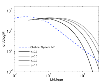
Given the similarity between the CMF and the IMF, some authors suggested an one-to-one conversion of dense cores into young stars (e.g., Lada et al., 2008). Although this scenario has been criticized on the basis of binary stars’ prevalence (see e.g., Smith et al., 2009), it is nonetheless informative to explore this simplest possibility. In this case, $P(m_{c},m^{*})=\delta(m^{*}-m_{c}\eta_{\rm sf}(m_{c}))$ (see Equation 6). $\eta_{\rm sf}$ is the retention factor, which is the fraction of core mass finally remained in the stars, for one particular core. While the more often loosely used phrase ‘star formation efficiency’ should refer to the global ratio of total stellar masses over total progenitor core masses, in a certain region and time-scale. In Figure 2 we show the IMFs generated with this model. We assume only cores with mass exceeding the Bonnor-Ebert mass can form stars, such that the star formation rate

$$\gamma_{\rm sf}(m_{c})=\begin{cases}0\ &{\rm if}\ m_{c}<m_{\rm BE}\cr\Gamma_{\rm sf}&{\rm if}\ m_{c}\geq m_{\rm BE}\cr\end{cases}$$ (7)

Here, $\Gamma_{\rm sf}=t_{\rm sf}^{-1}$ (see Equation 5) is the characteristic star formation rate. We also assume that the retention factor, i.e. the amount of the core mass retained in the resulting star, is assumed to be constant with a value $0<\eta_{\rm sf}(m_{c})<1$.

The results in Figure 2 show that the IMFs are shifted toward the low-mass end, with a broad peak near the original Bonnor-Ebert mass modified by the retention factor. With $\eta_{\rm sf}=0.3$ the new peak is at around $0.7~{}M_{\odot}$, which corresponds to Lada’s suggestion (Lada et al., 2008). The overall shape of the IMF resembles the observed stellar IMF. The low-mass end have similar dispersion with that of Chabrier’s IMF, provided the retention factor $\eta_{\rm sf}$ is not a sensitive function of the progenitor core mass. The high-mass end power-law is steeper than the Salpeter slope (Salpeter, 1955), where the observational uncertainty in this range is also relatively large. However, the minimum mass of stars we can produce with a single star formation prescript, is dependent on the critical Bonnor-Ebert mass, and $\eta_{\rm sf}$ such that $m_{\rm cut-off}\sim m_{\rm BE,new}\eta_{\rm sf}$. Due to this cut-off even with a low value of $\eta_{\rm sf}$ ($\eta_{\rm sf}=0.3$, dark grey line in Figure 2), this model has no inference for the lowest mass stars. The bulk of the modeled IMFs are more massive than the Chabrier IMF. We conclude that a non-unity retention factor alone would not explain the transition from CMF to IMF.

3.2. Case 2: Solely binary formation

A large fraction of the young stars are binaries. Each component of the binary contributes to the statistics of the IMF. Another limiting case of interest is the possibility that all the cores with mass in excess of the modified Bonnor-Ebert mass would fragment into binary stars. In principle, binary star formation is a consequence of rotational fragmentation and the kinematic properties are determined by the angular momentum distribution of the cores and their cooling ability. However, we are primarily interested in the IMF rather than the period distribution. We adopt an idealized power-law distribution for the mass ratio q such that

$$\frac{dn^{*}_{\rm binary}}{d\textit{q}}\propto\textit{q}^{-\beta}.$$ (8)

Here, the cut-off is taken as $\textit{q}_{\rm min}=0.05$. We explore a range of power-law indices $\beta$ between $0.2$ and $2.5$, which essentially covers the extreme limits. We assume a constant retention $\eta_{\rm sf}=0.3$ and star formation rate same as in Equation (7). The results here remain valid if the retention factor does not vary strongly with the progenitor core mass.

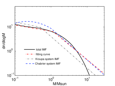
All the resulting IMFs with different $\beta$ display a broad shifted peak around the new, reduced Bonnor-Ebert mass (Figure 2). The results are very slightly affected by different $\beta$ in this wide range, so only $\beta=0.2$ is shown. The mass associated with the turn-over of the IMF is smaller than that found for the single star formation model. The segments in $0.46~{}M_{\odot}<m\leq 1.45~{}M_{\odot}$ with power-law index $\gamma_{1}=0.489$ and in $1.45~{}M_{\odot}<m\leq 10~{}M_{\odot}$ with power-law index $\gamma_{2}=1.5$. The two indices are quite similar to those of the piece-wise Kroupa IMF. We expect that the allowance of trinaries and quaternaries will further move the peak towards low-mass end.

3.3. Case 3: The binary companion’s IMF

In a classical study of the binary star population census by Duquennoy & Mayor (1991), the IMF for the companions of G-dwarf stars is thoroughly analyzed. They show that binaries on average can be formed by random combination of stars drawn from the same IMF. Following their basic approach, we consider the IMF of the primary and secondary stars separately. We assume all the progenitor cores fragment into binaries and the secondary star masses follow a distribution (e.g. Gaussian, Salpeter or Miller-Scalo (Miller & Scalo, 1979) power-law) independent of their primaries’ mass. For simplicity, we adopt a power-law, so the transfer functions as in Equation (6) become:

$$P_{\rm sec}(m_{\rm sec},m_{c})\propto dn_{\rm sec}/dm_{\rm sec}\propto(m_{\rm sec})^{-\alpha},$$ (9)

$$P_{\rm prim}(m_{\rm sec},m_{c})=P_{\rm sec}(\eta m_{c}-m_{\rm sec},m_{c}),$$ (10)

where the subscript ’sec’ and ’prim’ represent the secondary and the primary star. For $P_{\rm sec}$ the range of $m^{*}$is $0.08~{}M_{\odot}<m_{\rm sec}<0.5~{}\eta_{\rm sf}m_{c}$. The power-law index for the secondary star mass distribution, $\alpha$, varies from $0.8$ to $1.5$ in our calculations, while the star formation rate is as in Equation (7) and the retention factor $\eta_{\rm sf}=0.3$ is still assumed. Here, the IMF of the primary star preserves its characteristic broad peak and overall shape. The characteristic mass associated with this peak is smaller than that of the CMF.

The consequent IMF for the primary stars is very slightly influenced by $\alpha$ in this wide range, so we only show the result with $\alpha=1.5$ in Figure 2. Following Duquennoy & Mayor (1991), we compare the total (primary and secondary) simulated IMF with some well-known IMFs, such as the Kroupa IMF. The shape of the modeled IMF resembles the Kroupa IMF more closely at masses below $0.7~{}M_{\odot}$. We fit it with two broken power-laws. The low-mass end ($m<1~{}M_{\odot}$) completely reproduces the assumed power-law we put in, with $dn/d\log\,m=m^{-0.5}$, while the intermediate mass range ($1~{}M_{\odot}<m<10~{}M_{\odot}$) recover the Salpeter power-law $dn/d\log\,m=m^{-1.3}$.

3.4. Analytical results for the binary mass ratio distribution

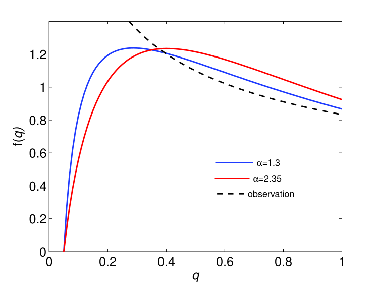
An alternative approach to characterize binary star statistics is to utilize the mass ratio, defined as $\textit{q}=m_{\rm sec}/m_{\rm prim}$. Observations show that the mass ratio also roughly follows a power-law distribution, as in Scorpius OB2 for intermediate mass stars (Kouwenhoven et al., 2007). Given a probability distribution of mass ratio $p(\textit{q}|m_{\rm core})$ in a binary formation process (formed from cores with mass $m_{\rm core}$), we can combine it with the CMF $p(m_{\rm core})$ to predict the mass ratio distribution $f(\textit{q})$:

$$p(\textit{q})=\int_{m_{\rm min}}^{m_{\rm max}}p(\textit{q}|m_{\rm core})p(m_{\rm core})dm_{\rm core}.$$ (11)

With a power-law mass distribution of the progenitor dense cores and an assumed constant retention, we can estimate the probability of finding a binary system with stellar masses of $m_{\rm prim}$ and $m_{\rm sec}$ to be

$$f(m_{\rm prim},m_{\rm sec})\propto(m_{\rm prim}+m_{\rm sec})^{-\alpha},$$ (12)

where $\alpha$ is the power-law index of the progenitor CMF. For random pairing of binary systems (Duquennoy & Mayor, 1991),

$$p\text{{q}}|m_{\rm core})=\frac{1}{1-\text{{q}}_{\rm min}}\ \ \ \ \>{\rm for}\text{{q}}\in[\text{{q}}_{\rm min},1]$$ (13)

with $\textsl{{q}}_{\rm min}$ as the minimum allowed binary ratio.

The cumulative probability $P(\textit{q}<x)$ for all the binary systems would then be

$$P(\textit{q}<x)=\int_{m_{\rm min}}^{xm_{\rm max}}\,dm_{\rm prim}\\ \int_{\frac{m_{\rm prim}}{x}}^{m_{\rm max}}\,dm_{\rm sec}f(m_{\rm prim},m_{\rm sec}).$$ (14)

Thus, the statistically averaged distribution of mass ratios q would be

$$f(\textit{q})\equiv\frac{dP(\textit{q})}{d\textit{q}}\propto\frac{1+(2-\alpha)\textit{q}+(1-\alpha)\textit{q}_{\rm min}^{2-\alpha}\textit{q}^{\alpha-2}}{(2-\alpha)(1+\textit{q})^{\alpha}}\\ -(1+\textit{q})^{1-\alpha},$$ (15)

where $m_{\rm max}(=\eta_{\rm sf}m_{core})$ is the upper limit for progenitor core mass. We choose $\alpha$ values corresponding to Kroupa’s IMF power-law indices. Although there are some uncertainties in the minimum allowed mass ratio, binary systems with q ratio around 0.05 or less has been observed so we adopt $\textit{q}_{\rm min}=0.05$ in the calculation. Results are shown in Figure 3 and compared with the observed power-law from Kouwenhoven et al. (2007). Although the distribution of q depends on the value of $\textit{q}_{\rm min}$, the power-law slope converges, for $\textit{q}>>0.05$, to the observed value.

4. Discussion and Conclusions

In this work, we continue our investigation on the origin of the stellar IMF. Based on the similarity between the observed stellar IMF and the CMF of dense starless cores in the Pipe nebula, we assume that they are closely connected. In Gritschneder & Lin (2012), we suggest that the cold cores of molecular gas are the byproducts of a thermal instability or the fragmentation of the a shocked shell and they are pressure confined by tenuous warm atomic medium. The CMF of these cores is the natural outcome of their collisional coagulation and their fragmentation due to their hydrodynamic interaction with the surrounding medium (H13). We also assume that these cores become unstable, undergo gravitational collapse, and evolve into protostars after their mass exceeds the Bonnor-Ebert mass.

Although this simple model reproduces the basic observed slopes of the stellar IMF, there is a factor-of-three offset between the stellar mass associated with the peak of the stellar IMF and that associated with the peak of the cores’ CMF. The main motivation of the investigation presented in this paper is to suggest a mechanism to account for this shift.

In Huang et al. (2013), we suggest that the peak of the CMF is essentially the Bonnor-Ebert mass of the cores. In typical molecular clouds such as the Pipe nebula, the Bonnor-Ebert mass is $>1~{}M_{\odot}$. In principle, cores less massive than the Bonnor-Ebert mass are stable and they do not turn into stars. Yet, many low-mass stars are formed in young stellar clusters.

In this work, we make an attempt to resolve the issues of 1) the offset between the mass associated with the peak of the CMF and the IMF, and 2) the prolific production of sub-solar type stars in molecular clouds. We demonstrate that the onset of first massive stars in these clouds photoionize and heat the surrounding medium without significantly changing the ionization fraction and temperature of the cores. This feedback effect largely increases the external pressure which confines the cores (by up to two orders of magnitude). This change leads to the compression of the cores and a reduction in their Bonnor-Ebert mass.

The collapse of cores with a mass greater than the modified Bonnor-Ebert mass (and less than the original Bonnor-Ebert mass) can now lead to the formation of a large population of sub-solar-mass stars. The stellar IMF generally preserves the shape of the Salpeter-like CMF with a significant lowering in the peak mass. The shape of the IMF (dispersion and high mass end slope) is not strongly modified by the formation of binary stars through rotational fragmentation. In our model, the inclusion of binary fragmentation during the collapse is essential for the production of stars with mass lower than the modified Bonnor-Ebert mass.

One implication of this induced star formation scenario is that the intrinsic age spread of the stellar cluster is naturally very small. In our analysis, we have adopted an idealized treatment of the retention efficiency (often loosely referred to as star formation efficiency). A mass dependence in the retention factor may lead to some modification in the IMF. We present several models for single and binary star populations. They generally reproduce the transition from the CMF to the IMF suggested by the observational data. A prolific production of triple and hierarchical systems may also lead to the formation of very low-mass stars.

Finally, these models are constructed with solar composition. In metal-deficient gas, such as protoglobular cluster clouds, the inability to cool may lead to a higher internal temperature and a higher Bonnor-Ebert mass in the cores. This feedback mechanism may be particularly important in triggering the formation of low-mass stars with lifespans in excess of 10 Gyr. We will further explore this possibility in the future.

5. Acknowledgements

We thank M.B.N. Kouwenhoven and C. Lada for useful conversations. DNCL acknowledges support by NASA through NNX08AL41G. MG acknowledges support from the Humboldt Foundation in form of a Feodor Lynen Fellowship.

References

- Anathpindika (2011) Anathpindika, S., 2011, New Astronomy, Volume 16, Issue 8, December 2011, pp 477–484
- André et al. (2010) André, P., Men’shchikov, A., Bontemps, S., et al. 2010, A&A, 518, L102
- Bonnell & Bate (2006) Bonnell, I & Bate, M. 2006, MNRAS, 370, 488
- Bonnor (1956) Bonnor, W. B. 1956, MNRAS, 116, 351
- Chabrier (2003) Chabrier, G. 2003, PASP, 115, 763
- Clark et al. (2008) Clark, P., Bonnel, I & Klessen, R. 2008, MNRAS, 386, 3
- Cowie & McKee (1977) Cowie, L. L., & McKee, C. F. 1977, ApJ, 211, 135
- Draine (2011) Draine, B. T. 2011, Physics of the interstellar and intergalactic medium, Princeton University Press
- Duquennoy & Mayor (1991) Duquennoy, A., & Mayor, M., 1991, A&A, 248,485
- Ebert (1955) Ebert, R. 1955, Zeitschrift fur Astrophysik, 37, 217
- Eggleton (1971) Eggleton, P. P. 1971, MNRAS, 151, 351
- Ferland et al. (1998) Ferland, G. J., Korista, K. T., Verner, D. A., et al. 1998, PASP, 110, 761
- Graham & Langer (1973) Graham, R., & Langer, W. D. 1973, ApJ, 179, 469
- Gritschneder & Lin (2012) Gritschneder, M., & Lin, D. N. C. 2012, ApJ, 754, L13
- Gritschneder et al. (2009) Gritschneder M., Naab T., Burkert A., et al., 2009, MNRAS, 393, 21
- Huang et al. (2013) Huang, X., Zhou, T., & Lin, D. N. C. 2013, ApJ, 769, 23
- Klessen (2011) Klessen, R. S. 2011, EAS Publications Series, 51, 133
- Kouwenhoven et al. (2007) Kouwenhoven, M. B. N., Brown, A. G. A., Portegies Zwart, S. F., et al. 2007, A&A, 474 , L77
- Könyves et al. (2010) Könyves, V., André, P., Men’shchikov, A., et al. 2010, A&A, 518, L106
- Kroupa (2002) Kroupa, P. 2002, Science, 295, 82
- Lada et al. (2008) Lada, C., Muench, A. A., Rathborne, J., et al, 2008, ApJ,672, 410
- Lazarian & Vishniac (1999) Lazarian, A., & Vishniac, E. T. 1999, ApJ, 517, 700
- Lin & Murray (2000) Lin, D. N. C., & Murray, S. D. 2000, ApJ, 540, 170
- McKee & Cowie (1977) McKee, C. F., & Cowie, L. L. 1977, ApJ, 215, 213
- Miller & Scalo (1979) Miller, G. E., & Scalo, J. M. 1979, ApJS, 41, 513–547.
- Murray et al. (1993) Murray, S. D., White, S. D. M., Blondin, J. M., & Lin, D. N. C. 1993, ApJ, 407, 588
- Murray & Lin (1996) Murray, S. D., & Lin, D. N. C. 1996, ApJ, 467, 728
- Nutter & Ward-Thompson (2007) Nutter, D., & Ward-Thompson, D. 2007, MNRAS, 374, 1413
- Ostriker (2011) Ostriker, E. C. 2011, Computational Star Formation, 270, 467
- Rathborne et al. (2009) Rathborne, J. M., Lada, C. J., Muench, A. A., et al. 2009, ApJ, 699, 742
- Salpeter (1955) Salpeter, E. E., 1955 ApJ, 121, 161.
- Smith et al. (2009) Smith, R. J., Clark, P. C., & Bonnell, I. A. 2009, MNRAS, 396, 830
- Spitzer (1978) Spitzer L., 1978, Physical processes in the interstellar medium. Wiley-Interscience, New York
- Strömgren (1939) Strömgren B., 1939, ApJ, 89, 526
- Weidner et al. (2011) Weidner, C., Kroupa, P.& Pflamm-Altenburg, J. 2011, MNRAS, 412, 979