Unbounded Bayesian Optimization via Regularization

Abstract

Bayesian optimization has recently emerged as a popular and efficient tool for global optimization and hyperparameter tuning. Currently, the established Bayesian optimization practice requires a user-defined bounding box which is assumed to contain the optimizer. However, when little is known about the probed objective function, it can be difficult to prescribe such bounds. In this work we modify the standard Bayesian optimization framework in a principled way to allow automatic resizing of the search space. We introduce two alternative methods and compare them on two common synthetic benchmarking test functions as well as the tasks of tuning the stochastic gradient descent optimizer of a multi-layered perceptron and a convolutional neural network on MNIST.

1 Introduction

Bayesian optimization has recently emerged as a powerful tool for the efficient global optimization of black box objective functions. Since the technique was introduced over 50 years ago, it has been applied for many different applications. Perhaps the most relevant application for the machine learning community is the automated tuning of algorithms [2, 13, 18, 21, 8]. However, the current state of the art requires the user to prescribe a bounding box within which to search for the optimum. Unfortunately, setting these bounds—often arbitrarily—is one of the main difficulties hindering the broader use of Bayesian optimization as a standard framework for hyperparameter tuning. For example, this obstacle was raised at the NIPS 2014 Workshop on Bayesian optimization as one of the open challenges in the field.

In the present work, we propose two methods that are capable of growing the search space as the optimization progresses. The first is a simple heuristic which regularly doubles the volume of the search space, while the second is a regularization method that is practical and easy to implement in any existing Bayesian optimization toolbox based on Gaussian Process priors over objective functions.

At a high level, the regularized method is born out of the observation that the only component of Bayesian optimization that currently requires a bounding box on the search space is the maximization of the acquisition function; this constraint is necessary because acquisition functions can have suprema at infinity. By using a non-stationary prior mean as a regularizer, we can exclude this possibility and use an unconstrained optimizer, removing the need for a bounding box.

1.1 Related work

Although the notion of using a non-trivial Gaussian process prior mean is not new, it is usually expected to encode domain expert knowledge or known structure in the response surface. Only one recent work, to the best of the authors’ knowledge, has considered using the prior mean as a regularization term and it was primarily to avoid selecting points along boundaries and in corners of the bounding box [19].

In this work we demonstrate that regulization can be used to carry out Bayesian optimization without a rigid bounding box. We further introduce a volume doubling baseline, which we compare to the regularization approach. While the regularized algorithms exhibit a much more homogeneous search behaviour (i.e. boundaries and corners are not disproportionately favoured), the volume doubling baseline performs very well in practice.

We begin with a brief review of Bayesian optimization with Gaussian processes in the next section, followed by an introduction to regularization via non-stationary prior means in Section 3, including visualizations that show that our proposed approaches indeed venture out of the initial user-defined bounding box. Section 4 reports our results on two synthetic benchmarking problems and two neural network tuning experiments.

2 Bayesian optimization

Consider the global optimization problem of finding a global maximizer $\mathbf{x}_{\star}\in\operatornamewithlimits{arg\,max}_{\mathbf{x}\in\mathbb{R}^{d}}f(\mathbf{x})$ of an unknown objective function $f:\mathbb{R}^{d}\mapsto\mathbb{R}$. In this work, the function $f$ is assumed to be a black-box for which we have no closed-form expression or gradient information. We further assume that $f$ is expensive to evaluate so we wish to locate the best possible input $\mathbf{x}$ with a relatively small budget of $N$ evaluations. Finally, the evaluations $y\in\mathbb{R}$ of the objective function are noise-corrupted observations, and for the remainder of this work, we assume a Gaussian noise distribution, $y\sim\mathcal{N}(f(\mathbf{x}),\sigma^{2})$. In contrast to typical Bayesian optimization settings, we do not assume the $\operatornamewithlimits{arg\,max}$ to be restricted to a bounded subset $\mathcal{X}\subset\mathbb{R}^{d}$.

Bayesian optimization is a sequential model-based approach which involves (i) maintaining a probabilistic surrogate model over likely functions given observed data; and (ii) selecting future query points according to a selection policy, which leverages the uncertainty in the surrogate to negotiate exploration of the search space and exploitation of current modes. The selection policy is represented by an acquisition function $\alpha_{n}:\mathbb{R}^{d}\mapsto\mathbb{R}$, where the subscript indicates the implicit dependence on the surrogate and, by extension, on the observed data $\mathcal{D}_{n}=\{(\mathbf{x}_{i},y_{i})\}_{i=1}^{n}$. More precisely, at iteration $n$: an input $\mathbf{x}_{n+1}$ is selected by maximizing the acquisition function $\alpha_{n}$; the black-box is queried and produces a noisy $y_{n+1}$; and the surrogate is updated in light of the new data point $(\mathbf{x}_{n+1},y_{n+1})$. Finally, after $N$ queries the algorithm must make a final recommendation $\hat{\mathbf{x}}_{N}$ which represents its best estimate of the optimizer.

2.1 Gaussian processes

In this work we prescribe a Gaussian process (GP) prior over functions [15]. When combined with a Gaussian likelihood, the posterior is also a GP and the Bayesian update can be computed analytically. Note that other surrogate models, such as random forests, have also been proposed in the model-based optimization literature [9].

A Gaussian process $\mathrm{GP}(\mu_{0},k)$ is fully characterized by its prior mean function $\mu_{0}:\mathbb{R}^{d}\mapsto\mathbb{R}$ and its positive-definite kernel, or covariance, function $k:\mathbb{R}^{d}\times\mathbb{R}^{d}\mapsto\mathbb{R}$. Given any finite collection of $n$ points $\mathbf{x}_{1:n}$, the values of $f(\mathbf{x}_{1}),\dots,f(\mathbf{x}_{n})$ are jointly Gaussian with mean $\mathbf{m}$, where $m_{i}:=\mu_{0}(\mathbf{x}_{i})$, and $n\times n$ covariance matrix $\mathbf{K}$, where $K_{ij}=k(\mathbf{x}_{i},\mathbf{x}_{j})$—hence the term covariance function.

Given the Gaussian likelihood model, the vector of concatenated observations $\mathbf{y}=y_{1:n}$ is also jointly Gaussian with covariance $\mathbf{K}+\sigma^{2}\mathbf{I}$. Therefore, at any arbitrary test location $\mathbf{x}$, we can query our surrogate model (the GP) for the function value $f(\mathbf{x})$ conditioned on observed data $\mathcal{D}_{n}$. The quantity $f(\mathbf{x})$ is a Gaussian random variable with the following mean $\mu_{n}(\mathbf{x})$ and marginal variance $\sigma^{2}_{n}(\mathbf{x})$

$$\mu_{n}(\mathbf{x}) =\mu_{0}(\mathbf{x})+\mathbf{k}(\mathbf{x})^{\mathsf{T}}(\mathbf{K}+\sigma^{2}\mathbf{I})^{-1}(\mathbf{y}-\mathbf{m})\,,$$ (1)

$$\sigma^{2}_{n}(\mathbf{x}) =k(\mathbf{x},\mathbf{x})-\mathbf{k}(\mathbf{x})^{\mathsf{T}}(\mathbf{K}+\sigma^{2}\mathbf{I})^{-1}\mathbf{k}(\mathbf{x})\,,$$ (2)

where $\mathbf{k}(\mathbf{x})$ is the vector of cross-covariance terms between $\mathbf{x}$ and $\mathbf{x}_{1:n}$. Throughout this work we use the squared exponential kernel

$$k_{\textsc{se}}(\mathbf{x},\mathbf{x}^{\prime}) =\theta_{0}\exp(-\tfrac{1}{2}r^{2}),$$ (3)

where $r=(\mathbf{x}-\mathbf{x}^{\prime})^{\mathsf{T}}\bm{\Lambda}^{-1}(\mathbf{x}-\mathbf{x}^{\prime})$ and $\bm{\Lambda}$ is a diagonal matrix of $d$ length scales $\theta_{1:d}$ and $\theta_{0}$ is the kernel amplitude. Collectively referred to as the hyperparemeter, $\bm{\theta}=\theta_{0:d}$ parameterizes the kernel function $k$. When the noise variance $\sigma^{2}$ is unknown, it can be added as a model hyperparameter as well. Similarly, the most common agnostic choice of prior mean is a constant bias $\mu_{0}(\mathbf{x})\equiv b$ which can also be added to $\bm{\theta}$.

Hyperparameter marginalization.

As in many regression tasks, the hyperparameter $\bm{\theta}$ must somehow be specified and has a dramatic effect on performance. Common tuning techniques such as cross-validation and maximum likelihood are either highly data-inefficient or run the risk of overfitting. Recently, a Bayesian treatment of the hyperparameters via Markov chain Monte Carlo has become standard practice in Bayesian optimization [18]. Similarly in the present work, we specify an uninformative prior on $\bm{\theta}$ and approximately integrate it by sampling from the posterior $p(\bm{\theta}|\mathcal{D}_{n})$ via slice sampling.

2.2 Acquisition functions

So far we have described the statistical model we use to represent our belief about the unknown objective $f$ given data $\mathcal{D}_{n}$, and how to update this belief given new observations. We have not described any mechanism or policy for selecting the query points $\mathbf{x}_{1:n}$. One could select these arbitrarily or by grid search but this would be wasteful; uniformly random search has also been proposed as a surprisingly good alternative to grid search [3]. There is, however, a rich literature on selection strategies that utilize the surrogate model to guide the sequential search, i.e. the selection of the next query point $\mathbf{x}_{n+1}$ given $\mathcal{D}_{n}$.

The key idea behind these strategies is to define an acquisition functions $\alpha:\mathbb{R}^{d}\mapsto\mathbb{R}$ which quantifies the promise of any point in the search space. The acquisition function is carefully designed to trade off exploration of the search space and exploitation of current promising neighborhoods. There are three common types of acquisition functions: improvement-based, optimistic, and information-based policies.

The improvement-based acquisition functions, probability and expected improvement (PI and EI, respectively), select the next point with the most probable and most expected improvement, respectively [12, 14]. On the other hand, the optimistic policy upper confidence bound (GP-UCB) measures, marginally for each test point $\mathbf{x}$, how good the corresponding observation $y$ will be in a low and fixed probability “good case scenario”—hence the optimism [20]. In contrast, there exist information-based methods such as randomized probability matching, also known as Thompson sampling [22, 16, 4, 11, 1], or the more recent entropy search methods [23, 5, 6]. Thompson sampling selects the next point according to the distribution of the optimum $\mathbf{x}_{\star}$, which is induced by the current posterior [16, 6, 17]. Meanwhile, entropy search methods select the point $\mathbf{x}$ that is expected to provide the most information towards reducing uncertainty about $\mathbf{x}_{\star}$.

In this work we focus our attention on EI, which is perhaps the most common acquisition function. With the GP surrogate model, EI has the following analytic expression

$$\alpha^{\textsc{EI}}_{n}(\mathbf{x})=(\mu_{n}(\mathbf{x})-\tau)\Phi\left(\frac{\mu_{n}(\mathbf{x})-\tau}{\sigma_{n}(\mathbf{x})}\right)+\sigma_{n}(\mathbf{x})\phi\left(\frac{\mu_{n}(\mathbf{x})-\tau}{\sigma_{n}(\mathbf{x})}\right),$$ (4)

where $\Phi$ and $\phi$ denote the standard normal cumulative distribution and density functions, respectively. Note however that the technique we outline in the next section can readily be extended to any Gaussian process derived acquisition function, including all those mentioned above.

3 Unbounded Bayesian optimization

3.1 Volume doubling

Our first proposed heuristic approach consists in expanding the search space regularly as the optimization progresses, starting with an initial user-defined bounding box. This method otherwise follows the standard Bayesian optimization procedure and optimizes within the bounding box that is available at the given time step $n$. This approach requires two parameters: the number of iterations between expansions and the growth factor $\gamma$. Naturally, to avoid growing the feasible space $\mathcal{X}$ by a factor that is exponential in $d$, the growth factor applies to the volume of $\mathcal{X}$. Finally, the expansion is isotropic about the centre of the domain. In this work, we double ($\gamma=2$) the volume every $3d$ evaluations (only after an initial latin hypercube sampling of $3d$ points).

3.2 Regularizing improvement policies

We motivate the regularized approach by considering improvement policies (e.g. EI); however, in the next section we show that this proposed approach can be applied more generally to all GP-derived acquisition functions. Improvement policies are a popular class of acquisition functions that rely on the improvement function

$$I(\mathbf{x})=(f(\mathbf{x})-\tau)\mathbb{I}[f(\mathbf{x})\geq\tau]$$ (5)

where $\tau$ is some target value to improve upon. Expected improvement then compute $\mathbb{E}[I(\mathbf{x})]$ under the posterior GP.

When the optimal objective value $f_{\star}$ is known and we set $\tau=f_{\star}$, these algorithms are referred to as goal seeking [10]. When the optimum is not known, it is common to use a proxy for $f_{\star}$ instead, such as the value of the best observation so far, $y^{+}$; or in the noisy setting, one can use either the maximum of the posterior mean or the value of the posterior at the incumbent $\mathbf{x}^{+}$, where $\mathbf{x}^{+}\in\operatornamewithlimits{arg\,max}_{\mathbf{x}\in\mathbf{x}_{1:n}}\mu_{n}(\mathbf{x})$.

In some cases, the above choice of target $\tau=y^{+}$ can lead to a lack of exploration, therefore it is common to choose a minimum improvement parameter $\xi>0$ such that $\tau=(1+\xi)y^{+}$ (for convenience here we assume $y^{+}$ is positive and in practice one can subtract the overall mean to make it so). Intuitively, the parameter $\xi$ allows us to require a minimum fractional improvement over the current best observation $y^{+}$. Previously, the parameter $\xi$ had always been chosen to be constant if not zero. In this work we propose to use a function $\xi:\mathbb{R}^{d}\mapsto\mathbb{R}^{+}$ which maps points in the space to a value of fractional minimum improvement. Following the same intuition, the function $\xi$ lets us require larger expected improvements from points that are farther and hence acts as a regularizer that penalizes distant points. The improvement function hence becomes:

$$I(\mathbf{x})=(f(\mathbf{x})-\tau(\mathbf{x}))\mathbb{I}[f(\mathbf{x})\geq\tau(\mathbf{x})],\quad\text{with}\quad\tau(\mathbf{x})=(1+\xi(\mathbf{x}))y^{+},$$ (6)

where the choice of $\xi(\mathbf{x})$ is discussed in Section 3.2.2.

3.2.1 Extension to general policies

In the formulation of the previous section, our method seems restricted to improvement policies. However, many recent acquisition functions of interest are not improvement-based, such as GP-UCB, entropy search, and Thompson sampling. In this section, we describe a closely related formulation that generalizes to all acquisition functions that are derived from a GP surrogate model.

Consider expanding our choice of non-stationary target $\tau$ in Equation (6)

$$I(\mathbf{x}) =(f(\mathbf{x})-y^{+}(1+\xi(\mathbf{x})))\mathbb{I}[f(\mathbf{x})\geq y^{+}(1+\xi(\mathbf{x}))]$$

$$=(f(\mathbf{x})-y^{+}\xi(\mathbf{x})-y^{+})\mathbb{I}[f(\mathbf{x})-y^{+}\xi(\mathbf{x})\geq y^{+}]$$

$$=(\tilde{f}(\mathbf{x})-y^{+})\mathbb{I}[\tilde{f}(\mathbf{x})\geq y^{+}]$$ (7)

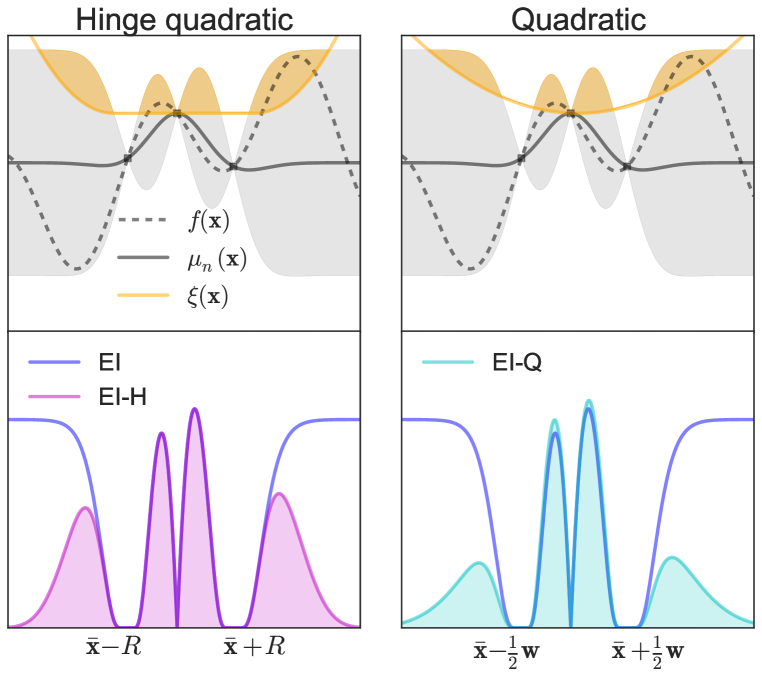
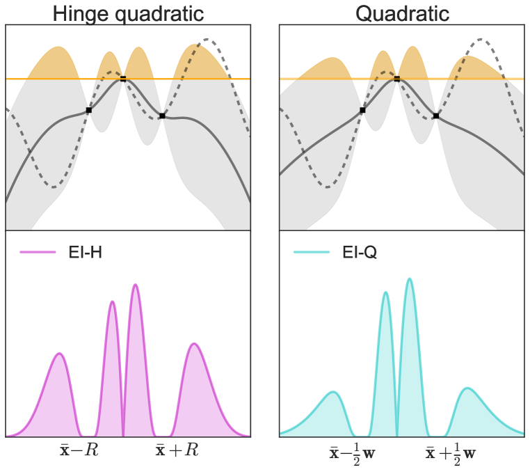
where $\tilde{f}$ is the posterior mean of a GP from (1) with prior mean $\tilde{\mu}_{0}(\mathbf{x})=\mu_{0}(\mathbf{x})-y^{+}\xi(\mathbf{x})$. Notice the similarity between (5) and (7). Indeed, in its current form we see that the regularization can be achieved simply by using a different prior mean $\tilde{\mu}_{0}$ and a constant target $y^{+}$. This duality can be visualized when comparing the left and right panel of Figure 1.

Precisely speaking, these two views are not exactly equivalent. Starting with the $\tilde{\mu}_{0}$ prior mean, the posterior mean yields an additional term

$$\mathbf{k}(\mathbf{x})^{\mathsf{T}}(\mathbf{K}+\sigma^{2}\mathbf{I})^{-1}\xi(\mathbf{X}),$$ (8)

where $[\xi(\mathbf{X})]_{i}=\xi(\mathbf{x}_{i})$. This term is negligible when the test point $\mathbf{x}$ is far from the data $\mathbf{X}$ due to our exponentially vanishing kernel, making the two alternate views virtually indistinguishable in Figure 1. However, with this new formulation we can apply the same regularization to any policy which uses a Gaussian process, e.g. Thompson sampling or entropy search.

3.2.2 Choice of regularization

By inspecting Equation (4), it is easy to see that any coercive prior mean function would lead to an asymptotically vanishing EI acquisition function; in this work however we consider quadratic (Q) and isotropic hinge-quadratic (H) regularizing prior mean functions, defined as follows (excluding the constant bias $b$)

$$\xi_{Q}(\mathbf{x}) =(\mathbf{x}-\bar{\mathbf{x}})^{\mathsf{T}}\mathrm{diag}(\mathbf{w}^{2})^{-1}(\mathbf{x}-\bar{\mathbf{x}}),$$ (9)

$$\xi_{H}(\mathbf{x}) =\mathbb{I}[\|\mathbf{x}-\bar{\mathbf{x}}\|_{2}>R]\frac{\|\mathbf{x}-\bar{\mathbf{x}}\|_{2}-R}{\beta R}.$$ (10)

Both of these regularizers are parameterized by $d$ location parameters $\bar{\mathbf{x}}$, and while $\xi_{Q}$ has an additional $d$ width parameters $\mathbf{w}$, the isotropic regularizer $\xi_{H}$ has a single radius $R$ and a single $\beta$ parameter, which controls the curvature of $\xi_{H}$ outside the ball of radius $R$; in what follows we fix $\beta=1$.

(a) Minimum improvement view

(b) Prior mean view

Figure 1: Visualization of the two alternate views of regularization in Bayesian optimization. The objective function and posterior surrogate mean are represented as black dashed and solid lines, respectively, with grey shaded areas indicating $\pm 2\sigma_{n}$. Integrating the surrogate model above the target (orange shaded area) results in the regularized EI acquisition function (magenta and cyan). Using a non-stationary target with a constant prior mean (left) or a fixed target with a non-stationary prior mean (right) lead to indistinguishable acquisition functions, which decay at infinity.

Fixed prior mean hyperparameters.

We are left with the choice of centre $\bar{\mathbf{x}}$ and radius parameters $R$ (or widths $\mathbf{w}$). Unlike the bias term $b$, these parameters of the regularizer are not intended to allow the surrogate to better fit the observations $\mathcal{D}_{n}$. In fact, using the marginal likelihood to estimate or marginalize $\psi=\{\bar{\mathbf{x}},R,\mathbf{w}\}$, could lead to fitting the regularizer to a local mode which could trap the algorithm in a suboptimal well. For this reason, we use an initial, temporary user-defined bounding box to set $\psi$ at the beginning of the run; the value of $\psi$ remains fixed in all subsequent iterations.

3.3 Visualization

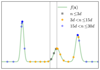
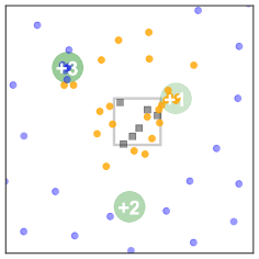
Before describing our experimental results, Figure 2 provides a visualization of EI with the hinge-quadratic prior mean, optimizing two toy problems in one and two dimensions. The objective functions consist of three Gaussian modes of varying heights and the initial bounding box does not include the optimum. We draw attention to the way the space is gradually explored outward from the initial bounding box.

Figure 2: Visualization of selections $\mathbf{x}_{n}$ made by the EI-H algorithm on two toy objective functions consisting of three Gaussian modes in one (left) and two (right) dimensions. Grey lines delimit the initial bounding box; grey square markers indicate the initial latin hypercube points, while the orange and blue points distinguish between the first and second half of the evaluation budget of $30d$, respectively. In the two-dimensional example, the height of the Gaussians are indicated by +1, +2, and +3.

4 Experiments

In this section, we evaluate our proposed methods and show that they achieve the desirable behaviour on two synthetic benchmarking functions, and a simple task of tuning the stochastic gradient descent and regularization parameters used in training a multi-layered perceptron (MLP) and a convolutional neural network (CNN) on the MNIST dataset.

Experimental protocol.

For every test problem of dimension $d$ and every algorithm, the optimization was run with an overall evaluation budget of $30d$ including an initial $3d$ points sampled according to a latin hypercube sampling scheme (as suggested in [10]). Throughout each particular run, at every iteration $n$ we record the value of the best observation up to $n$ and report these in Figure 3.

Algorithms.

We compared the two different methods from Section 3 to the standard EI with a fixed bounding box. Common random seeds were used for all methods in order to reduce confounding noise. All algorithms were implemented in the pybo framework available on github [7], and are labelled in our plots as follows:

EI:

Vanilla expected improvement with hyperparameter marginalization.

EI-V:

Expected improvement with the search volume doubled every $3d$ iterations.

EI-H/Q:

Regularized EI with a hinge-quadratic and quadratic prior mean, respectively.

Note that for the regularized methods EI-H/Q, the initial bounding box is only used to fix the location and scale of the regularizers, and to sample initial query points. In particular, both regularizers are centred around the box centre; for the quadratic regularizer the width of the box in each direction is used to fix $\mathbf{w}$, whereas for the hinge-quadratic $R$ is set to the box circumradius. Once these parameters are fixed, the bounding box is no longer relevant.

4.1 Synthetic benchmarks: Hartmann 3 and 6

The Hartmann 3 and 6 functions (numbers refer to their dimensionality) are standard, synthetic global optimization benchmarking test functions. In a separate experiment, indicated by an appended asterisk ($\ast$), we consider a randomly located bounding box of side length 0.2 within the unit hypercube. This window is unlikely to include the global optimum, especially in the six-dimensional problem, which makes this a good problem to test whether our proposed methods are capable of useful exploration outside the initial bounding box.

4.2 MLP and CNN on MNIST

The MNIST hand-written digit recognition dataset is a very common simple task for testing neural network methods and architectures. In this work we optimize the parameters of the stochastic gradient descent (SGD) algorithm used in training the weights of the neural network. In particular, we consider an MLP with 2048 hidden units with tanh non-linearities, and a CNN with two convolutional layers. These examples were taken from the official GitHub repository of torch7 demos. The code written for this work can be readily extended to any other demo in the repository or any torch script.

For this problem, we optimize four parameters, namely the learning rate and momentum of the SGD optimizer, and the $L_{1}$ and $L_{2}$ regularization coefficients. The parameters were optimized in log space (base $e$) with an initial bounding box of $[-3,-1]\times[-3,-1]\times[-3,1]\times[-3,1]$, respectively. For each parameter setting, a black-box function evaluation corresponds to training the network for one epoch and returning the test set accuracy. To be clear, the goal of this experiment is not to achieve state-of-the-art for this classification task but instead to demonstrate that our proposed algorithms can find optima well outside their initial bounding boxes.

4.3 Results

Figure 3: Best observations as optimization progresses. Plotting mean and standard error over 40 (Hartmann), 14 (MLP), and 19 (CNN) repetitions.

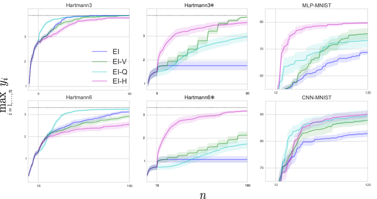
Figure 3 shows that for the Hartmann tests, the Bayesian optimization approaches proposed in this paper work well. The results confirm our hypothesis that the proposed methods are capable of useful exploration outside the initial bounding box. We note that when using the entire unit hypercube as the initial box, all the Bayesian optimization techniques exhibit similar performance as in this case the optimum is within the box. The Hartmann tests also show that our volume doubling heuristic is a good baseline method. Although it is less effective than EI-H as the dimensionality increases, it is nonetheless an improvement over standard EI in all cases.

The MNIST experiment shows good performance from all three methods EI-{V,H,Q}, particularly from the hinge-quadratic regularized algorithm. Indeed, when compared to the standard EI, EI-H boasts a 20% improvement in accuracy on the MLP and almost 10% on the CNN.

We believe that EI-H performs particularly well in settings where a small initial bounding box is prescribed because the hinge-quadratic regularizer allows the algorithm to explore outward more quickly. In contrast, EI-Q performs better when the optimum is included in the initial box; we suspect that this is due to the fact that the regularizer avoids selecting boundary and corner points, which EI and EI-V tend to do, as can be seen in Figure 4. Indeed, the green dots (EI-V) follow the corners of the growing bounding box. In contrast, EI-H/Q do not exhibit this artefact.

Figure 4: Pairwise scatterplot of selections (upper triangle) and recommendations (lower triangle) for the MLP-MNIST experiment. For example, the second plot of the first row corresponds to a scatter plot of the selected learning rates vs. momentum parameters for a single seed. In contrast, the first plot of the second row corresponds to a scatter plot of the recommended learning rates and momentum parameters over all 14 runs. The initial bounding box and sample points (for this particular run) are shown as a black rectangle and black square dots, respectively. All other points respect the color scheme of Figure 3. ($L_{2}$ cropped out for space.)

5 Conclusion and future work

In this work, we propose a versatile new approach to Bayesian optimization which is not limited to a search within a bounding box. Indeed, given an initial bounding box that does not include the optimum, we have demonstrated that our approach can expand its region of interest and achieve greater function values. Our method fits seamlessly within the current Bayesian optimization framework, and can be readily used with any acquisition function which is induced by a GP.

Finally, this could have implications in a distributed Bayesian optimization scheme whereby multiple Bayesian optimization processes are launched, each responsible for a neighbourhood of the domain. Interactions between these processes could minimize overlaps or alternatively ensure a certain level of redundancy, which would be helpful in a noisy setting.

We emphasize that in this work we have addressed one of the challenges that must be overcome toward the development of practical Bayesian optimization hyper-parameter tuning tools. A full solution, however, must also address the issues of dimensionality, non-stationarity, and early stopping. Fortunately, there has been great recent progess along these directions, and the methods proposed in this paper provide a complementary and essential piece of the puzzle.

References

- [1] S. Agrawal and N. Goyal. Thompson sampling for contextual bandits with linear payoffs. In International Conference on Machine Learning, 2013.
- [2] J. Bergstra, R. Bardenet, Y. Bengio, and B. Kégl. Algorithms for hyper-parameter optimization. In Advances in Neural Information Processing Systems, pages 2546–2554, 2011.
- [3] J. Bergstra and Y. Bengio. Random search for hyper-parameter optimization. Journal of Machine Learning Research, 13:281–305, 2012.
- [4] O. Chapelle and L. Li. An empirical evaluation of Thompson sampling. In Advances in Neural Information Processing Systems, pages 2249–2257, 2011.
- [5] P. Hennig and C. J. Schuler. Entropy search for information-efficient global optimization. The Journal of Machine Learning Research, pages 1809–1837, 2012.
- [6] J. M. Hernández-Lobato, M. W. Hoffman, and Z. Ghahramani. Predictive entropy search for efficient global optimization of black-box functions. In Advances in Neural Information Processing Systems. 2014.
- [7] M. W. Hoffman and B. Shahriari. Modular mechanisms for Bayesian optimization. In NIPS workshop on Bayesian Optimization, 2014.
- [8] M. W. Hoffman, B. Shahriari, and N. de Freitas. On correlation and budget constraints in model-based bandit optimization with application to automatic machine learning. In AI and Statistics, pages 365–374, 2014.
- [9] F. Hutter, T. Bartz-Beielstein, H. H. Hoos, K. Leyton-Brown, and K. P. Murphy. Sequential model-based parameter optimisation: an experimental investigation of automated and interactive approaches. In T. Bartz-Beielstein, M. Chiarandini, L. Paquete, and M. Preuss, editors, Empirical Methods for the Analysis of Optimization Algorithms, chapter 15, pages 361–411. Springer, 2010.
- [10] D. R. Jones. A taxonomy of global optimization methods based on response surfaces. J. of Global Optimization, 21(4):345–383, 2001.
- [11] E. Kaufmann, N. Korda, and R. Munos. Thompson sampling: An asymptotically optimal finite-time analysis. In Algorithmic Learning Theory, volume 7568 of Lecture Notes in Computer Science, pages 199–213. Springer Berlin Heidelberg, 2012.
- [12] Harold J Kushner. A new method of locating the maximum point of an arbitrary multipeak curve in the presence of noise. Journal of Fluids Engineering, 86(1):97–106, 1964.
- [13] N. Mahendran, Z. Wang, F. Hamze, and N. de Freitas. Adaptive MCMC with Bayesian optimization. Journal of Machine Learning Research - Proceedings Track, 22:751–760, 2012.
- [14] Jonas Močkus, V Tiesis, and Antanas Žilinskas. The application of bayesian methods for seeking the extremum. In L Dixon and G Szego, editors, Toward Global Optimization, volume 2. Elsevier, 1978.
- [15] C. E. Rasmussen and C. K. I. Williams. Gaussian Processes for Machine Learning. The MIT Press, 2006.
- [16] S. L. Scott. A modern Bayesian look at the multi-armed bandit. Applied Stochastic Models in Business and Industry, 26(6):639–658, 2010.
- [17] B. Shahriari, Z. Wang, M. W. Hoffman, A. Bouchard-Côté, and N. de Freitas. An entropy search portfolio. In NIPS workshop on Bayesian Optimization, 2014.
- [18] J. Snoek, H. Larochelle, and R. P. Adams. Practical Bayesian optimization of machine learning algorithms. In Advances in Neural Information Processing Systems, pages 2951–2959, 2012.
- [19] J. Snoek, O. Rippel, K. Swersky, R. Kiros, N. Satish, N. Sundaram, M. Patwary, M. Ali, R. P. Adams, et al. Scalable Bayesian optimization using deep neural networks. arXiv preprint arXiv:1502.05700, 2015.
- [20] N. Srinivas, A. Krause, S. M. Kakade, and M. Seeger. Gaussian process optimization in the bandit setting: No regret and experimental design. In International Conference on Machine Learning, pages 1015–1022, 2010.
- [21] K. Swersky, J. Snoek, and R. P. Adams. Multi-task Bayesian optimization. In Advances in Neural Information Processing Systems, pages 2004–2012, 2013.
- [22] W. R. Thompson. On the likelihood that one unknown probability exceeds another in view of the evidence of two samples. Biometrika, 25(3/4):285–294, 1933.
- [23] J. Villemonteix, E. Vazquez, and E. Walter. An informational approach to the global optimization of expensive-to-evaluate functions. J. of Global Optimization, 44(4):509–534, 2009.