Maximal stochastic transport in the Lorenz equations
Abstract
We calculate the stochastic upper bounds for the Lorenz equations using an extension of the background method. In analogy with Rayleigh-Bénard convection the upper bounds are for heat transport versus Rayleigh number. As might be expected, the stochastic upper bounds are larger than the deterministic counterpart of Souza and Doering (2015), but their variation with noise amplitude exhibits interesting behavior. Below the transition to chaotic dynamics the upper bounds increase monotonically with noise amplitude. However, in the chaotic regime this monotonicity depends on the number of realizations in the ensemble; at a particular Rayleigh number the bound may increase or decrease with noise amplitude. The origin of this behavior is the coupling between the noise and unstable periodic orbits, the degree of which depends on the degree to which the ensemble represents the ergodic set. This is confirmed by examining the close returns plots of the full solutions to the stochastic equations and the numerical convergence of the noise correlations. The numerical convergence of both the ensemble and time averages of the noise correlations is sufficiently slow that it is the limiting aspect of the realization of these bounds. Finally, we note that the full solutions of the stochastic equations demonstrate that the effect of noise is equivalent to the effect of chaos.
I Introduction
Noise is an integral part of any physical system. It can be ascribed to fluctuations arising from intermittent forcing, observational uncertainties, interference from external sources or unresolved physics. In circumstances where noise acts to destroy a signal of interest, it is viewed as a nuisance. However, it can also be the case that fluctuations act to stabilize a system, examples of which include noise-induced optical multi-stability Barbéroshie et al. (1993), asymmetric double well potentials Mankin et al. (2008), plant ecosystems D’Odorico et al. (2005), population dynamics Parker et al. (2011), and in electron-electron interactions in quantum systems Landauer (1998). Curiously, it has recently been shown that noise can have positive effects on cognitive functions such as learning and memory Rausch et al. (2013). Finally, a key issue arising when examining observational data is whether fluctuations are intrinsic or due to external forcing, which can be confounded by temporal multifractality (e.g., Agarwal et al., 2012).
Given the breadth of settings in which the effects of noise manifest themselves on dynamical systems, it appears prudent to examine such matters in a well studied and yet broadly relevant system. Thus, we study the influence of noise in the Lorenz system Lorenz (1963), which is an archetype of deterministic nonlinear dynamics. Moreover, Souza and Doering (2015) have recently determined the maximal (upper bounds) transport in the Lorenz equations, thereby providing us with a rigorous test bed for stochastic extensions. In §II we describe the stochastic Lorenz model, followed by the derivation of the stochastic upper bounds in §III. We interpret the core results and their implications in §IV before concluding.
II Stochastic Lorenz Model
The Lorenz model is a Galerkin-modal truncation of the equations for Rayleigh-Bénard convection with stress-free boundary conditions on the upper and lower boundaries. It acts as a rich toy model of low-dimensional chaos and since it’s origin extensive studies have been made spanning a wide range of areas (e.g., Strogatz, 2014). Of particular relevance here, is using the system as a model for heat transport in high Rayleigh number turbulent convection Souza and Doering (2015).
The stochastic form of the Lorenz system is described by the following coupled nonlinear ordinary differential equations,
| (1) | |||||
where describes the intensity of convective motion, the temperature difference between ascending and descending flow and the deviation from linearity of the vertical temperature profile. The control parameters are the Prandtl Number, the Rayleigh Number and a domain geometric factor. The are the noise amplitudes and are the noise processes. Clearly, the deterministic system has .
This type of additive noise may appear, for example, in observational errors, when the errors do not depend on the system state or as a model of sub-grid scale processes approximated by noise associated with unexplained physics Arnold et al. (2013). In multiplicative noise the system has an explicitly state dependent noise process.
Although real noise will always have a finite time correlation, taking the limit that the noise correlation goes to zero as , serves as a good approximation for the noise forcing. This is the white noise limit of colored noise forcing. White noise forcing is defined by an autocorrelation function written as
| (2) |
where, is the time lag, is the amplitude of the noise, represents the time average and is the Dirac delta-function.
III Stochastic Maximal Transport
Initiated by the work of Louis Howard Howard (1972), maximizing the transport of a quantity such as heat or mass is a core organizing principle in modern studies of dissipative systems. In this spirit Souza and Doering (2015) studied the transport in the deterministic Lorenz equations and determined the upper bound, which depends on the exact steady solutions , , as , where for . Moreover, they showed that any time-dependent forcing would decrease the transport in the system, and hence the steady state maximizes the transport in the system. We study the effect of noise on the maximal transport in this system as the Rayleigh number is varied.
Let and in the system of equations II, which transform to
| (3) | |||||
In the next two sub-sections, we calculate the stochastic upper bound of equations III using both Itô and Stratonovich calculi.
III.1 Itô Calculus Framework
Now, knowing that the state variables () in the Lorenz system are bounded Souza and Doering (2015); Doering and Gibbon (1995), and following the approach of Souza and Doering (2015) for this stochastic system, the long time averages of and can be written as
| (4) |
| (5) |
| (6) |
where, the terms in Eq. 4 and in Eq. 5 are a consequence of Itô’s lemma.
Now, let , where is time-independent Souza and Doering (2015), and equations 5 and 6 now become,
| (7) |
| (8) |
Therefore, equation (7) (8) becomes,
| (9) |
| (10) |
and adding to both sides gives,
| (11) |
We thus arrive at
| (12) | |||||
Comparing equation 12 above with equation from Souza and Doering (2015), we see an additional term due to the stochastic forcing
| (13) | |||||
which shows that the stochastic upper bound transcends the deterministic upper bound.
III.2 Stratonovich Calculus Framework
In this framework, the equations analogous to 4, 5 and 6 are
| (14) |
| (15) |
| (16) |
Again letting , where , equations 15 and 16 now become,
| (17) | |||||
| (18) |
| (19) | |||||
Now adding (14) to (19) we find
| (20) | |||||
Finally, adding to both sides gives
| (21) |
We thus arrive at
| (22) | |||||
Now, comparing Eq. 22 above with Eq. from Souza and Doering (2015), we see an additional term due to the stochastic forcing, which, as expected from the previous section, increases the upper bound;
| (23) | |||||
Due to the fact that the noise is additive, the upper-bounds from Itô and Stratonovich calculi should be equivalent. This is indeed the case because for the Itô result, , whereas for the Stratonovich result and . Therefore, when we take the ensemble average of equations 23 and 13 we obtain
| (24) |
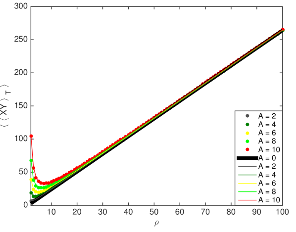
We plot equation 24 in Fig. 2, wherein the lines show the analytic solution and the solid circles denote the numerical solution, taking the ensemble average of equation 23, all as a function of noise amplitude .
IV Results & Interpretation
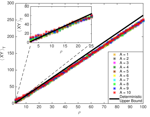
It is often the case that for the nonlinear dynamical systems found in nature, we only have a single time series. Thus, it is a natural question to ask about the properties of the stochastic upper bound both for the ensemble average and for a small number of realizations. Whereas deterministic chaos acts to decrease the transport in the system Souza and Doering (2015), here we find that it can also be indistinguishable from noise. In Fig. 1 we show individual realizations (one for each of 10 amplitudes ) of the transport as a function of . These exhibit two important features. (1) For below the deterministic transition to chaos (), the solutions transcend the deterministic upper bound (DUB), whereas for above they cross below it. (2) Independent of , there is no systematic dependence of the solutions on the noise amplitude. Taken together these features show that the impact of noise differs substantially depending on whether the deterministic dynamics is chaotic or non-chaotic. Clearly, the role of noise is indistinguishable from the role of chaotic dynamics and in individual realizations a given noise amplitude couples with various unstable periodic orbits, which we discuss in more detail below.
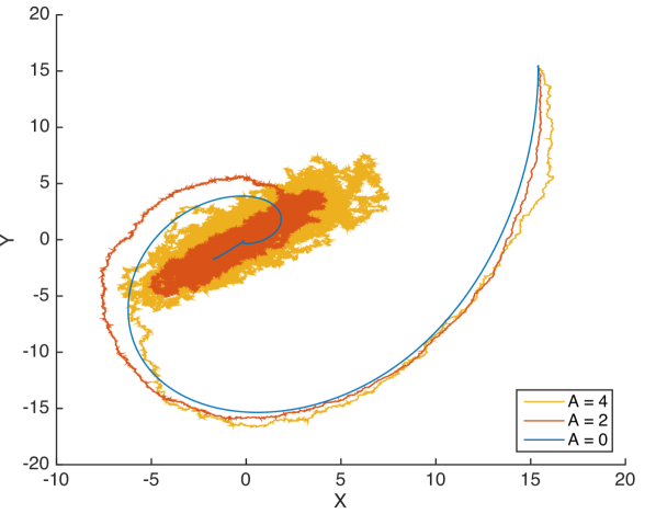
The analytical solution from equation 24 and the numerical solution (taking the ensemble average in equation 23) of the stochastic upper bound (SUB) are shown in Fig. 2. Firstly, we see the increase in the SUB as the noise amplitude increases. Secondly, for fixed amplitude and values of , the origin of the increase in the SUB are the two terms proportional to . As increases and decreases the SUB converges to the DUB from above. The increase with at low is a reflection of the dependence of the “diameter” of the system in the plane, other parameters being held constant. Because the diameter decreases as decreases, the relative influence of on the SUB is larger. We show this for in Fig. 3. However, we note that, using a different method Fantuzzi and Goluskin (pers. comm.) find a SUB that does not exhibit the low divergence, asymptotes to our bound for in the region of typical interest, and also recovers the DUB in the appropriate limit.
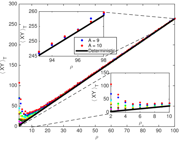
A more detailed view of the SUB from Eq. 23 is shown in Fig 4. The lower right inset shows that for the SUB is a monotonic function of the noise amplitude, as one would intuitively expect from Fig. 3. However, as the system enters the chaotic regime, this monotonicity is lost to reveal an oscillation with amplitude, as shown in the upper inset of Fig. 4 for noise amplitudes and . This oscillatory behavior is due to the coupling of noise with chaotic orbits that, depending on the amplitude, can result in different residence times of a trajectory in different orbits. Indeed, although for , the realization to realization stochastic upper bounds are consistent, this is not the case in the chaotic regime due to the coupling between the noise and the chaotic orbits. In consequence, each realization results in a slightly different SUB and hence the bound is not strict; it has a diffuseness that depends on the noise amplitude. This combined effect of noise and the exponential divergence property of chaos allows the noise to perturb the stochastic system into a different orbit in each realization.
The close returns plot of Mindlin and Gilmore (1992) can be used to extract unstable periodic orbits (UPO) from a chaotic time series. Thus, to demonstrate the coupling between noise and chaos discussed above in a different manner, we show the close returns plot for the stochastic Lorenz attractor (equation II) for and in Fig. 5 . These plots help us distinguish between noise and chaos. Whereas in a noisy system the points are more diffuse, in a chaotic system they are more structured, with continuous straight lines defining the UPOs.
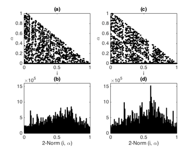
To further quantify this structure, in Fig. 5 we plot the histogram of the norm of the points from the close returns plot. The peaks in the histogram show the UPOs in the system, corresponding to the lines in the close returns plot. Whereas the histogram in Fig. 5 has a broad-band structure, that in Fig. 5 reveals prominent peaks at different norms.
V Summary
We calculated the stochastic upper bounds of the heat for the Lorenz equations using an extension of the background method of Souza and Doering (2015) used in the deterministic system. Whilst one might have expected that the stochastic upper bounds transcend their deterministic counterpart of Souza and Doering (2015), their variation with noise amplitude exhibits rich behavior. In the non-chaotic regime the upper bounds increase monotonically with noise amplitude. However, in the chaotic regime this monotonicity depends on the number of realizations in the ensemble; at a particular Rayleigh number the bound may increase or decrease with noise amplitude. The origin of this behavior is the coupling between the noise and unstable periodic orbits, the degree of which depends on the degree to which the ensemble represents the ergodic set. This is confirmed by examining the close returns plots of the full solutions to the stochastic equations. These solutions also demonstrate that the effect of noise is equivalent to the effect of chaos for a wide range of noise amplitude. Finally, we note that although in Itô-calculus the analytic bound (equation 24) relies on vanishing noise correlations (), numerically such correlations never completely vanish (e.g., Ito, 1984)111To test time convergence in the Itô Case we take the time average of these noise correlations for turnover times of 50 and 1550, and find that the magnitude of the correlations are of the same order; the correlations change from 0.05 (50 turnover times) to 0.015 (1550 turnover times). For the ensemble average convergence, with a single member the noise correlations are 0.05 (with 50 turnover times), and for 1000 members (with 50 turnover times) these are 0.001. Thus, both time and ensemble averages converge slowly with the latter being slightly superior., for as the size and diffuseness of stochastic attractor continually increases, the extent to which ensemble average reaches the ergodic set remains a concept rather than a practical reality.
Acknowledgements.
SA and JSW acknowledge NASA Grant NNH13ZDA001N-CRYO for support. JSW acknowledges the Swedish Research Council and a Royal Society Wolfson Research Merit Award for support. This work was completed whilst the authors were at the 2015 Geophysical Fluid Dynamics Summer Study Program at the Woods Hole Oceanographic Institution, which is supported by the National Science Foundation and the Office of Naval Research. We thank C.R. Doering, G. Fantuzzi, D. Goluskin and A. Souza for feedback.References
- Souza and Doering (2015) A. N. Souza and C. R. Doering, Phys. Lett. A 379, 518 (2015).
- Barbéroshie et al. (1993) A. Barbéroshie, I. Gontsya, Y. N. Nika, and A. K. Rotaru, Zh. Eksp. Teor. Fiz. 104, 2655 (1993).
- Mankin et al. (2008) R. Mankin, E. Soika, and A. Sauga, WSEAS Trans. Syst. 7, 239 (2008).
- D’Odorico et al. (2005) P. D’Odorico, F. Laio, and L. Ridolfi, Proc. Natl. Acad. Sci. USA 102, 10819 (2005).
- Parker et al. (2011) M. Parker, A. Kamenev, and B. Meerson, Phys. Rev. Lett. 107, 180603 (2011).
- Landauer (1998) R. Landauer, Nature 392, 658 (1998).
- Rausch et al. (2013) V. H. Rausch, E. M. Bauch, and N. Bunzeck, J. Cogn. Neuroscience 26, 1469 (2013).
- Agarwal et al. (2012) S. Agarwal, W. Moon, and J. S. Wettlaufer, Proc. Roy. Soc. Lond. A 468, 2416 (2012).
- Lorenz (1963) E. N. Lorenz, J. Atmos. Sci. 20, 130 (1963).
- Strogatz (2014) S. H. Strogatz, Nonlinear Dynamics and Chaos: With Applications to Physics, Biology, Chemistry, and Engineering, 2nd ed. (Westview Press, 2014).
- Arnold et al. (2013) H. M. Arnold, I. M. Moroz, and T. N. Palmer, Phil. Trans. R. Soc. A 371 (May 28, 2013).
- Howard (1972) L. N. Howard, Annu. Rev. Fl. Mech. 4, 473 (1972).
- Doering and Gibbon (1995) C. R. Doering and J. D. Gibbon, Dyn. Stab. Syst. 10, 255 (1995).
- Mindlin and Gilmore (1992) G. M. Mindlin and R. Gilmore, Physica D 58, 229 (1992).
- Ito (1984) H. M. Ito, J. Stat. Phys. 35, 151 (1984).
- Note (1) To test time convergence in the Itô Case we take the time average of these noise correlations for turnover times of 50 and 1550, and find that the magnitude of the correlations are of the same order; the correlations change from 0.05 (50 turnover times) to 0.015 (1550 turnover times). For the ensemble average convergence, with a single member the noise correlations are 0.05 (with 50 turnover times), and for 1000 members (with 50 turnover times) these are 0.001. Thus, both time and ensemble averages converge slowly with the latter being slightly superior.