Training Conditional Random Fields with Natural Gradient Descent

Abstract

We propose a novel parameter estimation procedure that works efficiently for conditional random fields (CRF). This algorithm is an extension to the maximum likelihood estimation (MLE), using loss functions defined by Bregman divergences which measure the proximity between the model expectation and the empirical mean of the feature vectors. This leads to a flexible training framework from which multiple update strategies can be derived using natural gradient descent (NGD). We carefully choose the convex function inducing the Bregman divergence so that the types of updates are reduced, while making the optimization procedure more effective by transforming the gradients of the log-likelihood loss function. The derived algorithms are very simple and can be easily implemented on top of the existing stochastic gradient descent (SGD) optimization procedure, yet it is very effective as illustrated by experimental results.

1 Introduction

Graphical models are used extensively to solve NLP problems. One of the most popular models is the conditional random fields (CRF) [Lafferty, 2001], which has been successfully applied to tasks like shallow parsing [Fei Sha and Fernando Pereira, 2003], name entity recognition [Andrew McCallum and Wei Li, 2003], word segmentation [Fuchun Peng et al. , 2004] etc., just to name a few.

While the modeling power demonstrated by CRF is critical for performance improvement, accurate parameter estimation of the model is equally important. As a general structured prediction problem, multiple training methods for CRF have been proposed corresponding to different choices of loss functions. For example, one of the common training approach is maximum likelihood estimation (MLE), whose loss function is the (negative) log-likelihood of the training data and can be optimized by algorithms like L-BFGS [Dong C. Liu and Jorge Nocedal, 1989], stochastic gradient descent (SGD) [Bottou, 1998], stochastic meta-descent (SMD) [Schraudolph, 1999] [Vishwanathan, 2006] etc. If the structured hinge-loss is chosen instead, then the Passive-Aggressive (PA) algorithm [Crammer et al., 2006], structured Perceptron [Collins, 2002] (corresponding to a hinge-loss with zero margin) etc. can be applied for learning.

In this paper, we propose a novel CRF training procedure. Our loss functions are defined by the Bregman divergence [Bregman, 1967] between the model expectation and empirical mean of the feature vectors, and can be treated as a generalization of the log-likelihood loss. We then use natural gradient descent (NGD) [Amari, 1998] to optimize the loss. Since for large-scale training, stochastic optimization is usually a better choice than batch optimization [Bottou, 2008], we focus on the stochastic version of the algorithms. The proposed framework is very flexible, allowing us to choose proper convex functions inducing the Bregman divergences that leads to better training performances.

In Section 2, we briefly reviews some background materials that are relevant to further discussions; Section 3 gives a step-by-step introduction to the proposed algorithms; Experimental results are given in Section 4, followed by discussions and conclusions.

2 Background

2.1 MLE for Graphical Models

Graphical models can be naturally viewed as exponential families [Wainwright and Jordan, 2008]. For example, for a data sample $(x,y)$ where $x$ is the input sequence and $y$ is the label sequence, the conditional distribution $p(y|x)$ modeled by CRF can be written as

$$p_{\boldsymbol{\theta}}(y|x)=\exp\{\boldsymbol{\theta}\cdot\boldsymbol{\Phi}(x,y)-A_{\boldsymbol{\theta}}\}$$

where $\boldsymbol{\Phi}(x,y)=\sum\limits_{c\in\mathcal{C}}\boldsymbol{\phi}_{c}(x_{c},y_{c})\in\mathbb{R}^{d}$ is the feature vector (of dimension $d$) collected from all factors $\mathcal{C}$ of the graph, and $A_{\boldsymbol{\theta}}$ is the log-partition function.

MLE is commonly used to estimate the model parameters $\boldsymbol{\theta}$. The gradient of the log-likelihood of the training data is given by

$$\widetilde{\mathbb{E}}-\mathbb{E}_{\boldsymbol{\theta}}$$ (1)

where $\widetilde{\mathbb{E}}$ and $\mathbb{E}_{\boldsymbol{\theta}}$ denotes the empirical mean of and model expectation of the feature vectors respectively. The moment-matching condition $\widetilde{\mathbb{E}}=\mathbb{E}_{\boldsymbol{\theta}^{*}}$ holds when the maximum likelihood solution $\boldsymbol{\theta}^{*}$ is found.

2.2 Bregman Divergence

The Bregman divergence is a general proximity measure between two points $\mathbf{p},\mathbf{q}$ (can be scalars, vectors, or matrices). It is defined as

$$B_{G}(\mathbf{p},\mathbf{q})=G(\mathbf{p})-G(\mathbf{q})-\nabla G(\mathbf{q})^{T}(\mathbf{p}-\mathbf{q})$$

where $G$ is a differentiable convex function inducing the divergence. Note that Bregman divergence is in general asymmetric, namely $B_{G}(\mathbf{p},\mathbf{q})\neq B(\mathbf{q},\mathbf{p})$.

By choosing $G$ properly, many interesting distances or divergences can be recovered. For example, choosing $G(\mathbf{u})=\frac{1}{2}\|\mathbf{u}\|^{2}$, $B_{G}(\mathbf{p},\mathbf{q})=\|\mathbf{p}-\mathbf{q}\|^{2}$ and the Euclidean distance is recovered; Choosing $G(\mathbf{u})=\sum\limits_{i}u_{i}\log u_{i}$, $B_{G}(\mathbf{p},\mathbf{q})=\sum\limits_{i}p_{i}\log\frac{p_{i}}{q_{i}}$ and the Kullback-Leibler divergence is recovered. A good review of the Bregman divergence and its properties can be found in [Banerjee et al., 2005].

2.3 Natural Gradient Descent

NGD is derived from the study of information geometry [Amari and Nagaoka, 2000], and is one of its most popular applications. The conventional gradient descent assumes the underlying parameter space to be Euclidean, nevertheless this is often not the case (say when the space is a statistical manifold). By contrast, NGD takes the geometry of the parameter space into consideration, giving an update strategy as follows:

$$\boldsymbol{\theta}_{t+1}=\boldsymbol{\theta}_{t}-\lambda_{t}M_{\boldsymbol{\theta}_{t}}^{-1}\nabla\ell(\boldsymbol{\theta}_{t})$$ (2)

where $\lambda_{t}$ is the learning rate and $M$ is the Riemannian metric of the parameter space manifold. When the parameter space is a statistical manifold, the common choice of $M$ is the Fisher information matrix, namely $M_{\boldsymbol{\theta}}^{i,j}=\mathbb{E}_{p}\left[\frac{\partial\log p_{\boldsymbol{\theta}}(x)}{\partial\theta_{i}}\frac{\partial\log p_{\boldsymbol{\theta}}(x)}{\partial\theta_{j}}\right]$. It is shown in [Amari, 1998] that NGD is asymptotically Fisher efficient and often converges faster than the normal gradient descent.

Despite the nice properties of NGD, it is in general difficult to implement due to the nontrivial computation of $M_{\boldsymbol{\theta}}^{-1}$. To handle this problem, researchers have proposed techniques to simplify, approximate, or bypass the computation of $M_{\boldsymbol{\theta}}^{-1}$, for example [Le Roux et al., 2007] [Honkela et al., 2008] [Pascanu and Bengio, 2013].

3 Algorithm

3.1 Loss Functions

The loss function defined for our training procedure is motivated by MLE. Since $\mathbb{E}_{\boldsymbol{\theta}}=\widetilde{\mathbb{E}}$ needs to hold when the solution to MLE is found, the “gap” between $\mathbb{E}_{\boldsymbol{\theta}}$ and $\widetilde{\mathbb{E}}$ (according to some measure) needs to be reduced as the training proceeds. We therefore define the Bregman divergence between $\mathbb{E}_{\boldsymbol{\theta}}$ and $\widetilde{\mathbb{E}}$ as our loss function. Since the Bregman divergence is in general asymmetric, we consider four types of loss functions as follows (named $B_{1}$-$B_{4}$):

$$B_{G}\left(\gamma\mathbb{E}_{\boldsymbol{\theta}},\widetilde{\mathbb{E}}-\rho\mathbb{E}_{\boldsymbol{\theta}}\right) (B_{1})$$

$$B_{G}\left(\widetilde{\mathbb{E}}-\rho\mathbb{E}_{\boldsymbol{\theta}},\gamma\mathbb{E}_{\boldsymbol{\theta}}\right) (B_{2})$$

$$B_{G}\left(\rho\widetilde{\mathbb{E}},\mathbb{E}_{\boldsymbol{\theta}}-\gamma\widetilde{\mathbb{E}}\right) (B_{3})$$

$$B_{G}\left(\mathbb{E}_{\boldsymbol{\theta}}-\gamma\widetilde{\mathbb{E}},\rho\widetilde{\mathbb{E}}\right) (B_{4})$$

where $\gamma\in\mathbb{R}$ and $\rho\triangleq 1-\gamma$. It can be seen that whenever the loss functions are minimized at point $\boldsymbol{\theta}^{*}$ (Bregman divergence reaches zero), $\mathbb{E}_{\boldsymbol{\theta}^{*}}=\widetilde{\mathbb{E}}$ and $\boldsymbol{\theta}^{*}$ give the same solution as MLE.

We are free to choose the hyper-parameter $\gamma$ which is possibly correlated with the performance of the algorithm. However to simplify the problem setting, we will only focus on the cases where $\gamma=0$ or $1$. Although it seems we now have eight versions of loss functions, it will be seen shortly that by properly choosing the convex function $G$, many of them are redundant and we end up having only two update strategies.

3.2 Applying Natural Gradient Descent

The gradients of loss functions $B_{1}$-$B_{4}$ with respect to $\boldsymbol{\theta}$ are given in Table 1.

Loss	Gradient wrt. $\boldsymbol{\theta}$	$\gamma$
$B_{1}$	$\nabla_{\boldsymbol{\theta}}\mathbb{E}_{\boldsymbol{\theta}}\left[\nabla G(\mathbb{E}_{\boldsymbol{\theta}})-\nabla G(\widetilde{\mathbb{E}})\right]$	$1$
	$\nabla_{\boldsymbol{\theta}}\mathbb{E}_{\boldsymbol{\theta}}\nabla^{2}G(\widetilde{\mathbb{E}}-\mathbb{E}_{\boldsymbol{\theta}})(\mathbb{E}_{\boldsymbol{\theta}}-\widetilde{\mathbb{E}})$	$0$
$B_{2}$	$\nabla_{\boldsymbol{\theta}}\mathbb{E}_{\boldsymbol{\theta}}\nabla^{2}G(\mathbb{E}_{\boldsymbol{\theta}})(\mathbb{E}_{\boldsymbol{\theta}}-\widetilde{\mathbb{E}})$	$1$
	$\nabla_{\boldsymbol{\theta}}\mathbb{E}_{\boldsymbol{\theta}}\left[\nabla G(\mathbf{0})-\nabla G(\widetilde{\mathbb{E}}-\mathbb{E}_{\boldsymbol{\theta}})\right]$	$0$
$B_{3}$	$\nabla_{\boldsymbol{\theta}}\mathbb{E}_{\boldsymbol{\theta}}\nabla^{2}G(\mathbb{E}_{\boldsymbol{\theta}}-\gamma\widetilde{\mathbb{E}})(\mathbb{E}_{\boldsymbol{\theta}}-\widetilde{\mathbb{E}})$	$\{0,1\}$
$B_{4}$	$\nabla_{\boldsymbol{\theta}}\mathbb{E}_{\boldsymbol{\theta}}\left[\nabla G(\mathbb{E}_{\boldsymbol{\theta}}-\gamma\widetilde{\mathbb{E}})-\nabla G(\rho\widetilde{\mathbb{E}})\right]$	$\{0,1\}$

Table 1: Gradients of loss functions $B_{1}$-$B_{4}$.

It is in general difficult to compute the gradients of the loss functions, as all of them contain the term $\nabla_{\boldsymbol{\theta}}\mathbb{E}_{\boldsymbol{\theta}}$, whose computation is usually non-trivial. However, it turns out that the natural gradients of the loss functions can be handled easily. To see this, note that for distributions in exponential family, $\nabla_{\boldsymbol{\theta}}\mathbb{E}_{\boldsymbol{\theta}}=\nabla_{\boldsymbol{\theta}}^{2}A_{\boldsymbol{\theta}_{t}}=M_{\boldsymbol{\theta}_{t}}$, which is the Fisher information matrix. Therefore the NGD update (Eq. 2) becomes

$$\boldsymbol{\theta}_{t+1}=\boldsymbol{\theta}_{t}-\lambda_{t}\nabla_{\boldsymbol{\theta}}\mathbb{E}_{\boldsymbol{\theta}_{t}}^{-1}\nabla\ell(\boldsymbol{\theta}_{t})$$ (3)

Now if we plug, for example $\nabla_{\boldsymbol{\theta}}B_{1},\gamma=0$, into Eq. 3, we have

$$\boldsymbol{\theta}_{t+1} = \boldsymbol{\theta}_{t}-\lambda_{t}\nabla_{\boldsymbol{\theta}}\mathbb{E}_{\boldsymbol{\theta}_{t}}^{-1}\nabla_{\boldsymbol{\theta}}B_{2}$$ (4)

$$= \boldsymbol{\theta}_{t}-\lambda_{t}\nabla^{2}G(\widetilde{\mathbb{E}}-\mathbb{E}_{\boldsymbol{\theta}_{t}})(\mathbb{E}_{\boldsymbol{\theta}_{t}}-\widetilde{\mathbb{E}})$$

Thus the step of computing the the Fisher information can be circumvented, making the optimization of our loss functions tractable.

This trick applies to all gradients in Table 1, yielding multiple update strategies. Note that $\nabla_{\boldsymbol{\theta}}B_{1},\gamma=1$ is equivalent to $\nabla_{\boldsymbol{\theta}}B_{4},\gamma=0$, and $\nabla_{\boldsymbol{\theta}}B_{2},\gamma=1$ is equivalent to $\nabla_{\boldsymbol{\theta}}B_{3},\gamma=0$. By applying Eq. 3 to all unique gradients, the following types of updates are derived (named $U_{1}$-$U_{6}$):

$$\boldsymbol{\theta}_{t+1}=\boldsymbol{\theta}_{t}-\lambda_{t}\nabla^{2}G(\widetilde{\mathbb{E}}-\mathbb{E}_{\boldsymbol{\theta}_{t}})(\mathbb{E}_{\boldsymbol{\theta}_{t}}-\widetilde{\mathbb{E}}) (U_{1})$$

$$\boldsymbol{\theta}_{t+1}=\boldsymbol{\theta}_{t}-\lambda_{t}\left[\nabla G(\mathbf{0})-\nabla G(\widetilde{\mathbb{E}}-\mathbb{E}_{\boldsymbol{\theta}_{t}})\right] (U_{2})$$

$$\boldsymbol{\theta}_{t+1}=\boldsymbol{\theta}_{t}-\lambda_{t}\nabla^{2}G(\mathbb{E}_{\boldsymbol{\theta}_{t}}-\widetilde{\mathbb{E}})(\mathbb{E}_{\boldsymbol{\theta}_{t}}-\widetilde{\mathbb{E}}) (U_{3})$$

$$\boldsymbol{\theta}_{t+1}=\boldsymbol{\theta}_{t}-\lambda_{t}\nabla^{2}G(\mathbb{E}_{\boldsymbol{\theta}_{t}})(\mathbb{E}_{\boldsymbol{\theta}_{t}}-\widetilde{\mathbb{E}}) (U_{4})$$

$$\boldsymbol{\theta}_{t+1}=\boldsymbol{\theta}_{t}-\lambda_{t}\left[\nabla G(\mathbb{E}_{\boldsymbol{\theta}_{t}}-\widetilde{\mathbb{E}})-\nabla G(\mathbf{0})\right] (U_{5})$$

$$\boldsymbol{\theta}_{t+1}=\boldsymbol{\theta}_{t}-\lambda_{t}\left[\nabla G(\mathbb{E}_{\boldsymbol{\theta}_{t}})-\nabla G(\widetilde{\mathbb{E}})\right] (U_{6})$$

3.3 Reducing the Types of Updates

Although the framework described so far is very flexible and multiple update strategies can be derived, it is not a good idea to try them all in turn for a given task. Therefore, it is necessary to reduce the types of updates and simplify the problem.

We first remove $U_{4}$ and $U_{6}$ from the list, since they can be recovered from $U_{3}$ and $U_{5}$ respectively by choosing $G^{\prime}(\mathbf{u})=G(\mathbf{u}+\widetilde{\mathbb{E}})$. To further reduce the update types, we impose the following constraints on the convex function $G$:

1. $G$ is symmetric: $G(\mathbf{u})=G(\mathbf{-u})$.

2. $\nabla G(\mathbf{u})$ is an element-wise function, namely $\nabla G(\mathbf{u})_{i}=g_{i}(u_{i}),\forall i\in 1,\ldots,d$, where $g_{i}$ is a uni-variate scalar function.

For example, $G(\mathbf{u})=\frac{1}{2}\|\mathbf{u}\|^{2}$ is a typical function satisfying the constraints, since $\frac{1}{2}\|\mathbf{u}\|^{2}=\frac{1}{2}\|-\mathbf{u}\|^{2}$, and $\nabla G(\mathbf{u})=[u_{1},\ldots,u_{d}]^{T}$ where $g_{i}(u)=u$, $\forall i\in 1,\ldots,d$. It is also worth mentioning that by choosing $G(\mathbf{u})=\frac{1}{2}\|\mathbf{u}\|^{2}$, all updates $U_{1}$-$U_{6}$ become equivalent:

$$\boldsymbol{\theta}_{t+1}=\boldsymbol{\theta}_{t}-\lambda_{t}\left(\mathbb{E}_{\boldsymbol{\theta}_{t}}-\widetilde{\mathbb{E}}\right)$$

which recovers the GD for the log-likelihood function.

When a twice-differentiable function $G$ satisfies the constraints 1 and 2, we have

$$\nabla G(\mathbf{u})=-\nabla G(\mathbf{-u})$$ (5)

$$\nabla G(\mathbf{0})=\mathbf{0}$$ (6)

$$\nabla^{2}G(\mathbf{u})=\nabla^{2}G(\mathbf{-u})$$ (7)

where Eq. 7 holds since $\nabla^{2}G$ is a diagonal matrix. Given these conditions, we see immediately that $U_{1}$ is equivalent to $U_{3}$, and $U_{2}$ is equivalent to $U_{5}$. This way, the types of updates are eventually narrowed down to $U_{1}$ and $U_{2}$.

To see the relationship between $U_{1}$ and $U_{2}$, note that the Taylor expansion of $\nabla G(\mathbf{0})$ at point $\widetilde{\mathbb{E}}-\mathbb{E}_{\boldsymbol{\theta}_{t}}$ is given by

$$\nabla G(\mathbf{0})= \nabla G(\widetilde{\mathbb{E}}-\mathbb{E}_{\boldsymbol{\theta}_{t}})+\nabla^{2}G(\widetilde{\mathbb{E}}-\mathbb{E}_{\boldsymbol{\theta}_{t}})(\mathbb{E}_{\boldsymbol{\theta}_{t}}-\widetilde{\mathbb{E}})$$

$$+O(\|\mathbb{E}_{\boldsymbol{\theta}_{t}}-\widetilde{\mathbb{E}}\|^{2})$$

Therefore $U_{1}$ and $U_{2}$ can be regarded as approximations to each other.

Since stochastic optimization is preferred for large-scale training, we replace $\widetilde{\mathbb{E}}$ and $\mathbb{E}_{\boldsymbol{\theta}_{t}}$ with its stochastic estimation $\widetilde{\mathbb{E}_{t}}$ and $\mathbb{E}_{\boldsymbol{\theta}_{t},t}$, where $\widetilde{\mathbb{E}_{t}}\triangleq\boldsymbol{\Phi}(x_{t},y_{t})$ and $\mathbb{E}_{\boldsymbol{\theta}_{t},t}\triangleq\mathbf{E}_{p_{\boldsymbol{\theta}_{t}}(Y|x_{t})}\left[\boldsymbol{\Phi}(x_{t},Y)\right]$. Assuming $G$ satisfies the constraints, we re-write $U_{1}$ and $U_{2}$ as

$$\boldsymbol{\theta}_{t+1}=\boldsymbol{\theta}_{t}-\lambda_{t}\nabla^{2}G(\mathbb{E}_{\boldsymbol{\theta}_{t},t}-\widetilde{\mathbb{E}_{t}})(\mathbb{E}_{\boldsymbol{\theta}_{t}}-\widetilde{\mathbb{E}_{t}}) (U_{1}^{*})$$

$$\boldsymbol{\theta}_{t+1}=\boldsymbol{\theta}_{t}-\lambda_{t}\nabla G(\mathbb{E}_{\boldsymbol{\theta}_{t},t}-\widetilde{\mathbb{E}_{t}}) (U_{2}^{*})$$

which will be the focus for the rest of the paper.

3.4 Choosing the Convex Function $G$

We now proceed to choose the actual functional forms of $G$ aiming to make the training procedure more efficient.

A naïve approach would be to choose $G$ from a parameterized convex function family (say the vector $p$-norm, where $p\geq 1$ is the hyper-parameter), and tune the hyper-parameter on a held-out set hoping to find a proper value that works best for the task at hand. However this approach is very inefficient, and we would like to choose $G$ in a more principled way.

Although we derived $U_{1}^{*}$ and $U_{2}^{*}$ from NGD, they can be treated as SGD of two surrogate loss functions $S_{1}(\boldsymbol{\theta})$ and $S_{2}(\boldsymbol{\theta})$ respectively (we do not even need to know what the actual functional forms of $S_{1}$, $S_{2}$ are), whose gradients $\nabla_{\boldsymbol{\theta}}S_{1}=\nabla^{2}G(\mathbb{E}_{\boldsymbol{\theta}}-\widetilde{\mathbb{E}})(\mathbb{E}_{\boldsymbol{\theta}}-\widetilde{\mathbb{E}})$ and $\nabla_{\boldsymbol{\theta}}S_{2}=\nabla G(\mathbb{E}_{\boldsymbol{\theta}}-\widetilde{\mathbb{E}})$ are transformations of the gradient of the log-likelihood (Eq. 1). Since the performance of SGD is sensitive to the condition number of the objective function [Bottou, 2008], one heuristic for the selection of $G$ is to make the condition numbers of $S_{1}$ and $S_{2}$ smaller than that of the log-likelihood. However, this is hard to analyze since the condition number is in general difficult to compute. Alternatively, we may select a $G$ so that the second-order information of the log-likelihood can be (approximately) incorporated, as second-order stochastic optimization methods usually converge faster and are insensitive to the condition number of the objective function [Bottou, 2008]. This is the guideline we follow in this section.

The first convex function we consider is as follows:

$$G_{1}(\mathbf{u})=\sum\limits_{i=1}^{d}\frac{u_{i}}{\sqrt{\epsilon}}\arctan(\frac{u_{i}}{\sqrt{\epsilon}})-\frac{1}{2}\log\left(1+\frac{u_{i}^{2}}{\epsilon}\right)$$

where $\epsilon>0$ is a small constant free to choose. It can be easily checked that $G_{1}$ satisfies the constraints imposed in Section 3.3. The gradients of $G_{1}$ are given by

$$\nabla G_{1}(\mathbf{u})=\frac{1}{\sqrt{\epsilon}}\left[\arctan(\frac{u_{1}}{\sqrt{\epsilon}}),\ldots,\arctan(\frac{u_{d}}{\sqrt{\epsilon}})\right]^{T}$$

$$\nabla^{2}G_{1}(\mathbf{u})=\text{diag}\left[\frac{1}{u_{1}^{2}+\epsilon},\ldots,\frac{1}{u_{d}^{2}+\epsilon}\right]$$

In this case, the $U_{1}^{*}$ update has the following form (named $U_{1}^{*}.G_{1}$):

$$\boldsymbol{\theta}_{t+1}^{i}=\boldsymbol{\theta}_{t}^{i}-\lambda_{t}\left[\left(\mathbb{E}_{\boldsymbol{\theta}_{t},t}^{i}-\widetilde{\mathbb{E}_{t}}^{i}\right)^{2}+\epsilon\right]^{-1}\left(\mathbb{E}_{\boldsymbol{\theta}_{t},t}^{i}-\widetilde{\mathbb{E}_{t}}^{i}\right)$$

where $i=1,\ldots,d$. This update can be treated as a stochastic second-order optimization procedure, as it scales the gradient Eq. 1 by the inverse of its variance in each dimension, and it reminds us of the online Newton step (ONS) [Hazan et al., 2007] algorithm, which has a similar update step. However, in contrast to ONS where the full inverse covariance matrix is used, here we only use the diagonal of the covariance matrix to scale the gradient vector. Diagonal matrix approximation is often used in optimization algorithms incorporating second-order information (for example SGN-QN [Bordes et al., 2009], AdaGrad [Duchi et al., 2011] etc.), as it can be computed orders-of-magnitude faster than using the full matrix ,without sacrificing much performance.

The $U_{2}^{*}$ update corresponding to the choice of $G_{1}$ has the following form (named $U_{2}^{*}.G_{1}$):

$$\boldsymbol{\theta}_{t+1}^{i}=\boldsymbol{\theta}_{t}^{i}-\lambda_{t}\arctan\left(\frac{\mathbb{E}_{\boldsymbol{\theta}_{t},t}^{i}-\widetilde{\mathbb{E}_{t}}^{i}}{\sqrt{\epsilon}}\right)$$

Note that the constant $1/\sqrt{\epsilon}$ in $\nabla G_{1}$ has been folded into the learning rate $\lambda_{t}$. Although not apparent at first sight, this update is in some sense similar to $U_{1}^{*}.G_{1}$. From $U_{1}^{*}.G_{1}$ we see that in each dimension, gradients $\mathbb{E}_{\boldsymbol{\theta}_{t}}^{i}-\widetilde{\mathbb{E}_{t}}^{i}$ with smaller absolute values get boosted more dramatically than those with larger values (as long as $|\mathbb{E}_{\boldsymbol{\theta}_{t}}^{i}-\widetilde{\mathbb{E}_{t}}^{i}|$ is not too close to zero). A similar property also holds for $U_{2}^{*}.G_{1}$, since arctan is a sigmoid function, and as long as we choose $\epsilon<1$ so that

$$\frac{d}{du}\arctan\left(\frac{1}{\sqrt{\epsilon}}u\right)\rvert_{u=0}=\frac{1}{\sqrt{\epsilon}}>1$$

the magnitude of $\mathbb{E}_{\boldsymbol{\theta}_{t}}^{i}-\widetilde{\mathbb{E}_{t}}^{i}$ with small absolute value will also get boosted. This is illustrated in Figure 1 by comparing functions $\frac{u}{u^{2}+\epsilon}$ (where we select $\epsilon=0.1$) and $\arctan\left(\frac{1}{\sqrt{\epsilon}}u\right)$. Note that for many NLP tasks modeled by CRF, only indicator features are defined. Therefore the value of $\mathbb{E}_{\boldsymbol{\theta}_{t}}^{i}-\widetilde{\mathbb{E}_{t}}^{i}$ is bounded by -1 and 1, and we only care about function values on this interval.

Figure 1: Comparison of functions $u/(u^{2}+0.1)$, arctan, erf, gd. The sigmoid functions arctan, erf and gd are normalized so that they have the same gradient as $u/(u^{2}+0.1)$ at $u=0$ and their values are bounded by -1, 1.

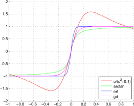
Since arctan belongs to the sigmoid function family, it is not the only candidate whose corresponding update mimics the behavior of $U_{1}^{*}.G_{1}$, while $G$ still satisfies the constraints given in Section  3.3. We therefore consider two more convex functions $G_{2}$ and $G_{3}$, whose gradients are the erf and Gudermannian functions (gd) from the sigmoid family respectively:

$$\nabla G_{2}(\alpha\mathbf{u})_{i}=\frac{2}{\pi}\int_{0}^{\alpha u_{i}}\exp\{-{x^{2}}\}dx$$

$$\nabla G_{3}(\beta\mathbf{u})_{i}=2\arctan(\exp\{\beta u_{i}\})-\frac{\pi}{2}$$

where $\alpha,\beta\in\mathbb{R}$ are hyper-parameters. In this case, we do not even know the functional form of the functions $G_{2}$, $G_{3}$, however it can be checked that both of them satisfy the constraints. The reason why we select these two functions from the sigmoid family is that when the gradients of erf and d are the same as that of arctan at point zero, both of them stay on top of arctan. Therefore, erf and gd are able to give stronger boosts to small gradients. This is also illustrated in Figure 1.

Applying $\nabla G_{2}$ and $\nabla G_{3}$ to $U_{2}^{*}$, we get two updates named $U_{2}^{*}.G_{2}$ and $U_{2}^{*}.G_{3}$ respectively. We do not consider further applying $\nabla^{2}G_{2}$ and $\nabla^{3}G_{3}$ to $U_{1}^{*}$, as the meaning of the updates becomes less clear.

3.5 Adding Regularization Term

So far we have not considered adding regularization term to the loss functions yet, which is crucial for better generalization. A common choice of the regularization term is the 2-norm (Euclidean metric) of the parameter vector $\frac{C}{2}\|\boldsymbol{\theta}\|^{2}$, where $C$ is a hyper-parameter specifying the strength of regularization. In our case, however, we derived our algorithms by applying NGD to the Bregman loss functions, which assumes the underlying parameter space to be non-Euclidean. Therefore, the regularization term we add has the form $\frac{C}{2}\boldsymbol{\theta}^{T}M_{\boldsymbol{\theta}}\boldsymbol{\theta}$, and the regularized loss to be minimized is

$$\frac{C}{2}\boldsymbol{\theta}^{T}M_{\boldsymbol{\theta}}\boldsymbol{\theta}+B_{i}$$ (8)

where $B_{i},i=\{1,2,3,4\}$ are the loss functions $B_{1}$-$B_{4}$.

However, the Riemannian metric $M_{\boldsymbol{\theta}}$ itself is a function of $\boldsymbol{\theta}$, and the gradient of the objective at time $t$ is difficult to compute. Instead, we use an approximation by keeping the Riemannian metric fixed at each time stamp, and the gradient is given by $M_{\boldsymbol{\theta}_{t}}\boldsymbol{\theta}_{t}+\nabla_{\boldsymbol{\theta}_{t}}B_{i}$. Now if we apply NGD to this objective, the resulting updates will be no different than the SGD for L2-regularized surrogate loss functions $S_{1}$, $S_{2}$:

$$\boldsymbol{\theta}_{t+1}=(1-C\lambda_{t})\left(\boldsymbol{\theta}_{t}-\frac{\lambda_{t}}{1-C\lambda_{t}}\nabla_{\boldsymbol{\theta}}{S_{i,t}(\boldsymbol{\theta}_{t})}\right)$$

where $i=\{1,2\}$. It is well-known that SGD for L2-regularized loss functions has an equivalent but more efficient sparse update [Shalev-Schwartz et al. , 2007] [Bottou, 2012]:

$$\bar{\boldsymbol{\theta}}_{t}=\frac{\boldsymbol{\theta}_{t}}{z_{t}}$$

$$\bar{\boldsymbol{\theta}}_{t+1}=\bar{\boldsymbol{\theta}}_{t}-\frac{\lambda_{t}}{(1-\lambda_{t})z_{t}}\nabla_{\boldsymbol{\theta}}{S_{i,t}(\boldsymbol{\theta}_{t})}$$

$$z_{t+1}=(1-C\lambda_{t})z_{t}$$

where $z_{t}$ is a scaling factor and $z_{0}=1$. We then modify $U_{1}^{*}$ and $U_{2}^{*}$ accordingly, simply by changing the step-size and maintaining a scaling factor.

As for the choice of learning rate $\lambda_{t}$, we follow the recommendation given by [Bottou, 2012] and set $\lambda_{t}=\left[\hat{\lambda}(1+\hat{\lambda}Ct)\right]^{-1}$, where $\hat{\lambda}$ is calibrated from a small subset of the training data before the training starts.

The final versions of the algorithms developed so far are summarized in Figure 2.

0:  

  Choose hyper-parameters $C$, $\epsilon/\alpha/\beta$ (depending on which convex function to use: $G_{1}$, $G_{2}$, $G_{3}$).Set $z_{0}=1$, and calibrate $\hat{\lambda}$ on a small training subset.

  

  for $e=1\ldots\texttt{num epoch}$ do

     for $t=1\ldots T$ do

        Receive training sample $(x_{t},y_{t})$

        $\lambda_{t}=\left[\hat{\lambda}(1+\hat{\lambda}Ct)\right]^{-1}$, $\boldsymbol{\theta}_{t}=z_{t}\bar{\boldsymbol{\theta}}_{t}$

        Depending on the update strategy selected, update the parameters:

        $\bar{\boldsymbol{\theta}}_{t+1}=\bar{\boldsymbol{\theta}}_{t}-\frac{\lambda_{t}}{(1-\lambda_{t})z_{t}}\nabla_{\boldsymbol{\theta}}{S_{t}(\boldsymbol{\theta}_{t})}$

        where $\nabla_{\boldsymbol{\theta}}{S_{t}(\boldsymbol{\theta}_{t})}_{i},i=1,\ldots,d$ is given by

        

$$\left[\left(\mathbb{E}_{\boldsymbol{\theta}_{t},t}^{i}-\widetilde{\mathbb{E}_{t}}^{i}\right)^{2}+\epsilon\right]^{-1}\left(\mathbb{E}_{\boldsymbol{\theta}_{t},t}^{i}-\widetilde{\mathbb{E}_{t}}^{i}\right) (U_{1}^{*}.G_{1})$$

$$\texttt{arctan}\left(\frac{\mathbb{E}_{\boldsymbol{\theta}_{t},t}^{i}-\widetilde{\mathbb{E}_{t}}^{i}}{\sqrt{\epsilon}}\right) (U_{2}^{*}.G_{1})$$

$$\texttt{erf}\left(\alpha(\mathbb{E}_{\boldsymbol{\theta}_{t},t}^{i}-\widetilde{\mathbb{E}_{t}}^{i})\right) (U_{2}^{*}.G_{2})$$

$$\texttt{gd}\left(\beta(\mathbb{E}_{\boldsymbol{\theta}_{t},t}^{i}-\widetilde{\mathbb{E}_{t}}^{i})\right) (U_{2}^{*}.G_{3})$$

        $z_{t+1}=(1-C\lambda_{t})z_{t}$

        

        if no more improvement on training set then

           exit

        end if

     end for

  end for

Figure 2: Summary of the proposed algorithms.

3.6 Computational Complexity

The proposed algorithms simply transforms the gradient of the log-likelihood, and each transformation function can be computed in constant time, therefore all of them have the same time complexity as SGD ($O(d)$ per update). In cases where only indicator features are defined, the training process can be accelerated by pre-computing the values of $\nabla^{2}G$ or $\nabla G$ for variables within range $\left[-1,1\right]$ and keep them in a table. During the actual training, the transformed gradient values can be found simply by looking up the table after rounding-off to the nearest entry. This way we do not even need to compute the function values on the fly, which significantly reduces the computational cost.

4 Experiments

4.1 Settings

We conduct our experiments based on the following settings:

Implementation: We implemented our algorithms based on the CRF suite toolkit [Okazaki, 2007], in which SGD for the log-likelihood loss with L2 regularization is already implemented. This can be easily done since our algorithm only requires to modify the original gradients. Other parts of the code remain unchanged.

Task: Our experiments are conducted for the widely used CoNLL 2000 chunking shared task [Sang and Buchholz, 2000]. The training and test data contain 8939 and 2012 sentences respectively. For fair comparison, we ran our experiments with two standard linear-chain CRF feature sets implemented in the CRF suite. The smaller feature set contains 452,755 features, whereas the larger one contains 7,385,312 features.

Baseline algorithms: We compare the performance of our algorithms summarized in Figure 2 with SGD, L-BFGS, and the Passive-Aggressive (PA) algorithm. Except for L-BFGS which is a second-order batch-learning algorithm, we randomly shuffled the data and repeated experiments five times.

Hyper-parameter selection: For convex function $G_{1}$ we choose $\epsilon=0.1$, correspondingly the arctan function in $U_{2}^{*}.G_{1}$ is $\arctan(3.16u)$. We have also experimented the function $\arctan(10u)$ for this update, following the heuristic that the transformation function $\frac{u}{u^{2}+0.1}$ given by $\nabla^{2}G_{1}$ and $\arctan(10u)$ have consistent gradients at zero, since the $U_{2}^{*}$ update imitates the behavior of $U_{1}^{*}$ (the two choices of the arctan functions are denoted by arctan.1 and arctan.2 respectively). Following the same heuristic, we choose $\alpha=5\sqrt{\pi}\approx 8.86$ for the erf function and $\beta=10$ for the gd function.

4.2 Results

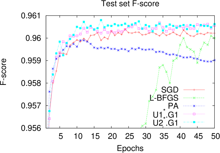
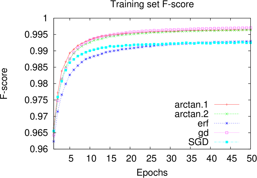
Comparison with the baseline: We compare the performance of the proposed and baseline algorithms on the training and test sets in Figure 3 and Figure 4, corresponding to small and large feature sets respectively. The plots show the F-scores on the training and test sets for the first 50 epochs. To keep the plots neat, we only show the average F-scores of repeated experiments after each epoch, and omit the standard deviation error bars. For $U_{2}^{*}.G_{1}$ update, only $\arctan.1$ function is reported here. From the figure we observe that:

1. The strongest baseline is given by SGD. By comparison, PA appears to overfit the training data, while L-BFGS converges very slowly, although eventually it catches up.

2. Although the SGD baseline is already very strong (especially with the large feature set), both the proposed algorithm $U_{1}^{*}.G_{1}$ and $U_{2}^{*}.G_{1}$ outperform SGD and stay on top of the SGD curves most of the time. On the other hand, the $U_{2}^{*}.G_{1}$ update appears to be a little more advantageous than $U_{1}^{*}.G_{1}$.

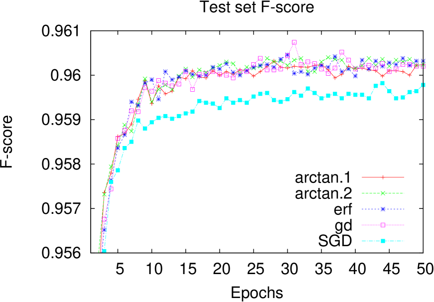
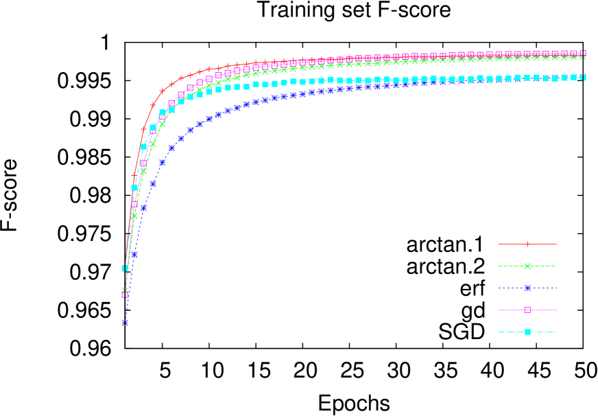
Comparison of the sigmoid functions: Since arctan, erf and gd are all sigmoid functions and it is interesting to see how their behaviors differ, we compare the updates $U_{2}^{*}.G1$ (for both $\arctan.1$ and $\arctan.2$), $U_{2}^{*}.G_{2}$ and $U_{2}^{*}.G_{3}$ in Figure 5 and Figure 6. The strongest baseline, SGD, is also included for comparison. From the figures we have the following observations:

1. As expected, the sigmoid functions demonstrated similar behaviors, and performances of their corresponding updates are almost indistinguishable. $U_{2}^{*}.G_{2}$. Similar to $U_{2}^{*}.G1$, $U_{2}^{*}.G2$ and $U_{2}^{*}.G3$ both outperformed the SGD baseline.

2. Performances of $U_{2}^{*}.G1$ given by arctan functions are insensitive to the choice of the hyper-parameters. Although we did not run similar experiments for erf and gd functions, similar properties can be expected from their corresponding updates.

Figure 3: F-scores of training and test sets given by the baseline and proposed algorithms, using the small feature set.

Figure 4: F-scores of training and test sets given by the baseline and proposed algorithms, using the large feature set.

Figure 5: F-scores of training and test sets given by $U_{2}^{*}.G1$, $U_{2}^{*}.G1$ and $U_{2}^{*}.G3$, using the small feature set.

Figure 6: F-scores of training and test sets given by $U_{2}^{*}.G1$, $U_{2}^{*}.G1$ and $U_{2}^{*}.G3$, using the large feature set.

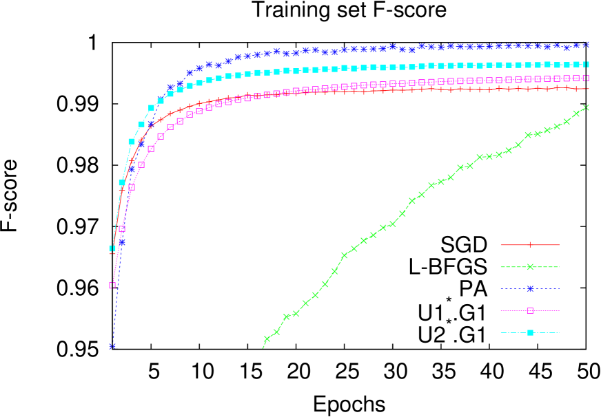
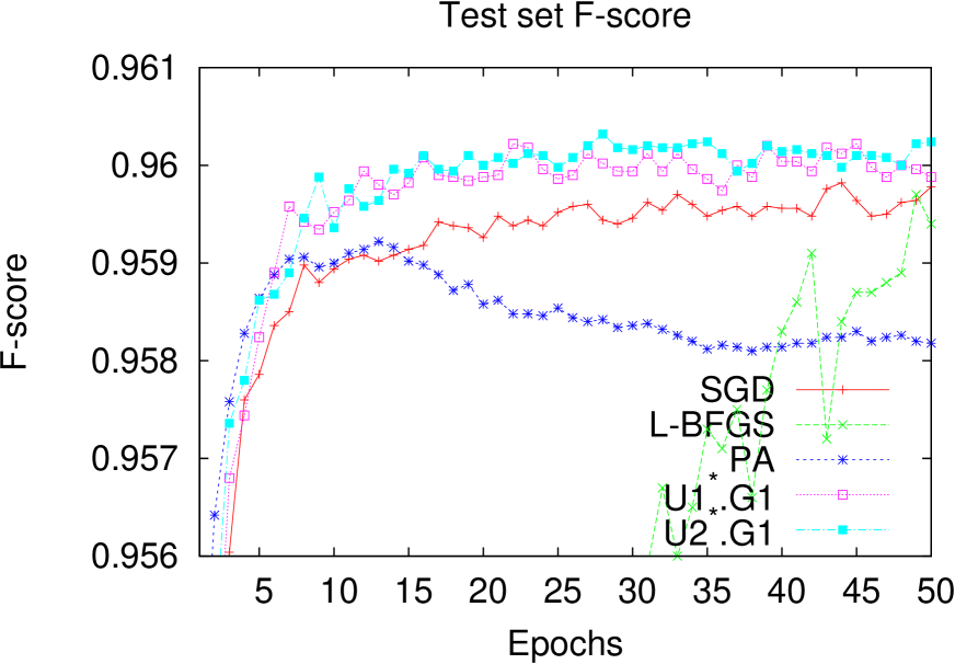
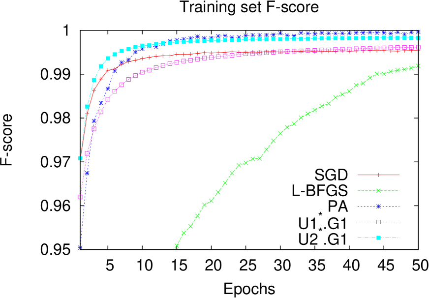
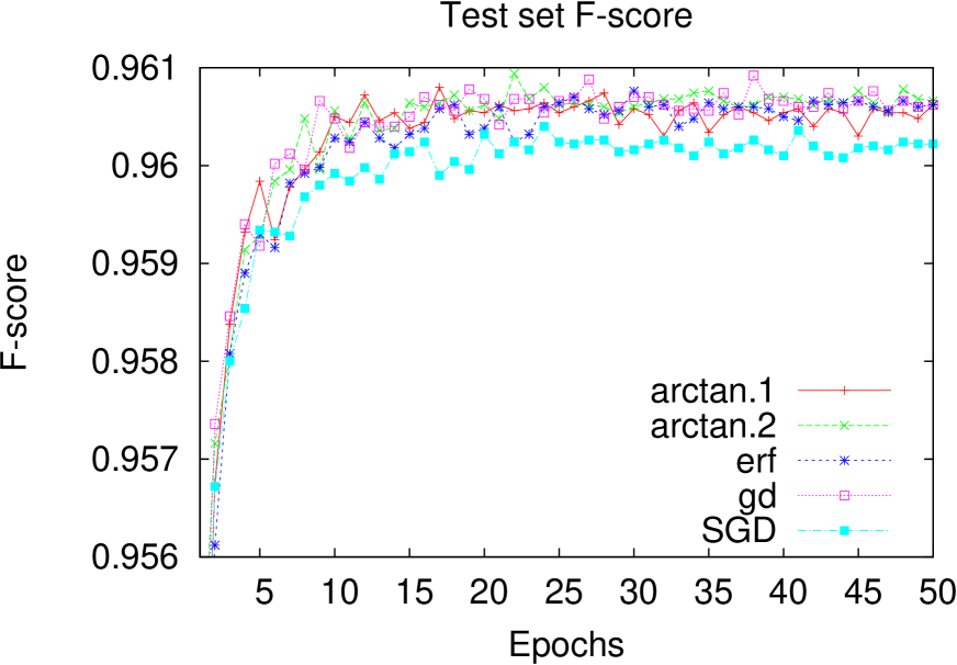
Finally, we report in Table 2 the F-scores on the test set given by all algorithms after they converge.

Algorithm	F-score % (small)	F-score % (large)
SGD	95.98$\pm$0.02	96.02$\pm$0.01
PA	95.82$\pm$0.04	95.90$\pm$0.03
L-BFGS	96.00	96.01
$U_{1}^{*}.G_{1}$	95.99$\pm$0.02	96.06$\pm$0.03
$U_{2}^{*}.G_{1}$	96.02$\pm$0.02	96.06$\pm$0.02
$U_{2}^{*}.G_{1}^{\prime}$	96.03 $\pm$ 0.01	96.06$\pm$0.03
$U_{2}^{*}.G_{2}$	96.03$\pm$0.02	96.06$\pm$0.02
$U_{2}^{*}.G_{3}$	96.02$\pm$0.02	96.06$\pm$0.02

Table 2: F-scores on the test set after algorithm converges, using the small and large feature sets. $U_{2}^{*}.G_{1}$ is the update given by arctan.1, and $U_{2}^{*}.G_{2}$ given by arctan.2.

5 Conclusion

We have proposed a novel parameter estimation framework for CRF. By defining loss functions using the Bregman divergences, we are given the opportunity to select convex functions that transform the gradient of the log-likelihood loss, which leads to more effective parameter learning if the function is properly chosen. Minimization of the Bregman loss function is made possible by NGD, thanks to the structure of exponential families. We developed several parameter update strategies which approximately incorporates the second-order information of the log-likelihood, and outperformed baseline algorithms that are already very strong on a popular text chunking task.

Proper choice of the convex functions is critical to the performance of the proposed algorithms, and is an interesting problem that merits further investigation. While we selected the convex functions with the motivation to reduce the types of updates and incorporate approximate second-order information, there are certainly more possible choices and the performance could be improved via careful theoretical analysis. On the other hand, instead of choosing a convex function apriori, we may rely on some heuristics from the actual data and choose a function tailored for the task at hand.

References

- [Amari, 1998] Shunichi Amari. 1998. Natural Gradient Descent Works Efficiently in Learning. Neural Computation, Vol. 10
- [Amari and Nagaoka, 2000] Shunichi Amari and Hiroshi Nagaoka. 2000. Methods of Information Geometry. The American Mathematical Society
- [Banerjee et al., 2005] Arindam Banerjee, Srujana Merugu, Inderjit S. Dhillon, Joydeep Ghosh. 2005. Clustering with Bregman Divergences. Journal of Machine Learning Research, Vol. 6, 1705–1749
- [Bordes et al., 2009] Antoine Bordes, Léon Bottou, and Patrick Gallinari. 2009. SGD-QN: Careful Quasi-Newton Stochastic Gradient Descent. Journal of Machine Learning Research, 10:1737–1754
- [Bottou, 1998] Léon Bottou. 1998. Online Algorithms and Stochastic Approximations. Online Learning and Neural Networks, Cambridge University Press
- [Bottou, 2008] Léon Bottou and Olivier Bousquet. 2008 The Tradeoffs of Large Scale Learning. Proceedings of Advances in Neural Information Processing Systems (NIPS), Vol. 20, 161–168
- [Bottou, 2012] Léon Bottou. 2012. Stochastic Gradient Descent Tricks. Neural Networks: Tricks of the Trade, Second Edition, Lecture Notes in Computer Science, Vol. 7700
- [Bregman, 1967] L. M. Bregman. 1967. The Relaxation Method of Finding the Common Points of Convex Sets and its Application to the Solution of Problems in Convex Programming. USSR Computational Mathematics and Mathematical Physics, 7(3):200–217
- [Collins, 2002] Michael Collins. 2002. Discriminative training methods for hidden Markov Models: Theory and Experiments with Perceptron. Algorithms Proceedings of Empirical Methods in Natural Language Processing (EMNLP), 10:1–8.
- [Crammer et al., 2006] Koby Crammer, Ofer Dekel, Joseph Keshet, Shai Shalev-Schwartz, and Yoram Singer. 2006. Online Passive-Aggressive Algorithms Journal of Machine Learning Research(JMLR), 7:551–585.
- [Duchi et al., 2011] John Duchi, Elad Hazan and Yoram Singer. 2011. Adaptive Subgradient Methods for Online Learning and Stochastic Optimization. Journal of Machine Learning Research, 12:2121-2159
- [Hazan et al., 2007] Elad Hazan, Amit Agarwal and Satyen Kale. 2007. Logarithmic Regret Algorithms for Online Convex Optimization. Machine Learning, Vol. 69, 169–192
- [Hoffman et al., 2013] Matthew D. Hoffman and David M. Blei and Chong Wang and John Pasley. 2013. Stochastic Variational Inference. Journal of Machine Learning Research, Vol. 14, 169–192
- [Honkela et al., 2008] Antti Honkela, Matti Tornio, Tapani Raiko and Juha Karhunen. 2008. Natural Conjugate Gradient in Variational Inference. Lecture Notes in Computer Science, Vol. 4985, 305–314
- [Lafferty, 2001] John Lafferty, Andrew McCallum and Fernando Pereira. 2001. Conditional Random Fields: Probabilistic Models for Segmenting and Labeling Sequence Data. Proceedings of International Conference on Machine Learning (ICML), 282–289
- [Le Roux et al., 2007] Nicolas Le Roux, Pierre-Antoine Manzagol and Yoshua Bengio. 2007. Topmoumoute Online Natural Gradient Algorithm. Proceedings of Advances in Neural Information Processing Systems (NIPS), 849–856
- [Dong C. Liu and Jorge Nocedal, 1989] Dong C. Liu and Jorge Nocedal. 1989. On the Limited Memory Method for Large Scale Optimization. Mathematical Programming, 45:503-528
- [Andrew McCallum and Wei Li, 2003] Andrew McCallum and Wei Li. 2003. Early Results for Named Entity Recognition with Conditional Random Fields, Feature Induction and Web-Enhanced Lexicons. Proceedings of the Seventh Conference on Natural Language Learning at NAACL-HLT, 188–191
- [Okazaki, 2007] Naoaki Okazaki. 2007. CRFsuite: A Fast Implementation of Conditional Random Fields (CRFs). http://www.chokkan.org/software/crfsuite
- [Pascanu and Bengio, 2013] Razvan Pascanu and Yoshua Bengio. 2013. Revisiting Natural Gradient for Deep Networks. arXiv preprint arXiv:1301.3584,
- [Fuchun Peng et al. , 2004] Fuchun Pent, Fangfang Feng and Andrew McCallum. 2004. Chinese Segmentation and New Word Detection Using Conditional Random Fields Proceedings of the International Conference on Computational Linguistics (COLING), 562–569
- [Sang and Buchholz, 2000] Erik F. Tjong Kim Sang and Sabine Buchholz. 2000. Introduction to the CoNLL-2000 Shared Task: Chunking Proceedings of Conference on Computational Natural Language Learning (CoNLL), Vol. 7, 127–132
- [Schraudolph, 1999] Nicol N. Schraudolph. 1999. Local Gain Adaptation in Stochastic Gradient Descent. Proceedings of International Conference on Artificial Neural Networks (ICANN), Vol. 2, 569–574
- [Shalev-Schwartz et al. , 2007] Shalev-Schwartz, Yoram Singer and Nathan Srebro. 2007. Pegasos: Primal Estimated sub-GrAdient SOlver for SVM. Proceedings of International Conference on Machine Learning (ICML), 807–814
- [Fei Sha and Fernando Pereira, 2003] Sha Fei and Fernando Pereira. 2003. Shallow Parsing with Conditional Random Fields Proceedings of North American Chapter of the Association for Computational Linguistics - Human Language Technologies (NAACL-HLT), 134–141
- [Vishwanathan, 2006] S.V. N. Vishwanathan, Nicol N. Schraudolph, Mark W. Schmidt and Kevin P. Murphy. 1999. Accelerated Training of Conditional Random Fields with Stochastic Gradient Methods. Proceedings of International Conference on Machine Learning (ICML), 969–976
- [Wainwright and Jordan, 2008] Martin J. Wainwright and Michael I. Jordan. 2008. Graphical Models, Exponential Families, and Variational Inference. Foundations and Trends in Machine Learning, Vol 1. 1-305