Parameter-space metric for all-sky semicoherent searches for
gravitational-wave pulsars

Karl Wette karl.wette@aei.mpg.de Max-Planck-Institut für Gravitationsphysik (Albert-Einstein-Institut), Callinstraße 38, 30167 Hannover, Germany
(2015-10-28 17:36:55 +0100; commitID: 2ded9fa-CLEAN)
Abstract

The sensitivity of all-sky searches for gravitational-wave pulsars is primarily limited by the finite availability of computing resources. Semicoherent searches are a widely-used method of maximizing sensitivity to gravitational-wave pulsars at fixed computing cost: the data from a gravitational-wave detector are partitioned into a number of segments, each segment is coherently analyzed, and the analysis results from each segment are summed together. The generation of template banks for the coherent analysis of each segment, and for the summation, requires knowledge of the metrics associated with the coherent and semicoherent parameter spaces respectively. We present a useful approximation to the semicoherent parameter-space metric, analogous to that presented in Wette and Prix [Phys. Rev. D 88, 123005 (2013)] for the coherent metric. The new semicoherent metric is compared to previous work in Pletsch [Phys. Rev. D 82, 042002 (2010)], and Brady and Creighton [Phys. Rev. D 61, 082001 (2000)]. We find that semicoherent all-sky searches require orders of magnitude more templates than previously predicted.

pacs:
04.80.Nn, 95.55.Ym, 95.75.Pq, 97.60.Jd

I Introduction

Gravitational-wave pulsars 111 As noted in Cutler (2012), the term “gravitational-wave pulsar” is a slight misnomer, since the signals they emit are more accurately described as “sinusoidal” than “pulsating”. are rotating neutron stars which are hypothesized, though not yet observed, to emit gravitational radiation in the form of long-lived, continuous, quasisinusoidal signals. The maximum amplitude of a gravitational-wave pulsar signal has been most recently studied in Johnson-McDaniel and Owen (2013), and the evolution of the population of Galactic neutron stars emitting at an assumed amplitude has been modeled in Knispel and Allen (2008); Wade et al. (2012). The sensitivity of the interferometric gravitational-wave observatories LIGO Abbott et al. (2009); Harry et al. (2010) and Virgo Accadia et al. (2012); Acernese et al. (2015) are expected to improve significantly within this decade, while a third large-scale observatory, KAGRA Somiya (2012), is under construction. Nevertheless, it remains likely that gravitational-wave pulsars will remain at best marginally detectable for the foreseeable future.

The detection of a gravitational-wave pulsar, in the absence of an observed electromagnetic counterpart (cf. Aasi et al., 2014), is a significant data-analysis challenge, requiring both large-scale computing resources and highly-optimized data analysis algorithms. The former is provided by the distributed computing project Einstein@Home 222 http://www.einsteinathome.org/. , which is dedicated to searching for both gravitational-wave and electromagnetic pulsars; to date, the project has discovered many new radio and gamma-ray pulsars (e.g. Knispel et al., 2013; Pletsch et al., 2013). Research into the latter has led to advances in the understanding of optimal and/or robust detection statistics (e.g. Jaranowski et al., 1998; Prix and Krishnan, 2009; Dergachev, 2010; Cutler, 2012; Keitel et al., 2014), the construction of matched-filtering template banks (e.g. Brady et al., 1998; Prix, 2007a, b; Messenger et al., 2009; Wette and Prix, 2013; Wette, 2014; Pisarski and Jaranowski, 2015), hierarchical search methods (e.g. Brady and Creighton, 2000; Krishnan et al., 2004; Pletsch, 2010) and their optimization given limited computing resources (e.g. Cutler et al., 2005; Prix and Shaltev, 2012), the estimation of search sensitivity (e.g. Wette, 2012), and pipelines for post-processing promising detection candidates (e.g. Shaltev and Prix, 2013; Behnke et al., 2015).

This paper builds on recent work on all-sky, broadband, coherent searches for isolated gravitational-wave pulsars. (Similar studies of the parameter-space metric for gravitational-wave pulsars in binary systems can be found in e.g. Messenger (2011); Leaci and Prix (2015).) In Wette and Prix (2013) (hereafter Paper I), a useful approximation to the parameter-space metric is developed, which is important for the correct construction of banks of matched-filtering templates. Previous work (e.g. Astone et al., 2002; Pletsch and Allen, 2009) had assumed restrictions on the time-span of data which could be coherently analyzed; these restrictions were relaxed in Paper I. In Wette (2014) (hereafter Paper II), a practical implementation of an optimal template bank using lattice template placement is presented. The number of templates in the bank was found to be in good agreement with the prediction of Brady et al. (1998).

This paper presents a useful approximation to the parameter-space metric for all-sky semicoherent searches for gravitational-wave pulsars, building on the work of Paper I. In a semicoherent search, the data are divided into a number of segments, each of which are coherently searched using a per-segment coherent template bank; the search results from each segment are then summed together using a semicoherent template bank 333 The terms “coarse template bank” and “fine template bank” are also used to refer to the coherent and semicoherent template banks respectively, e.g. in Prix and Shaltev (2012). . Each semicoherent template preserves a consistent (instantaneous) signal frequency f(t)𝑓𝑡f(t) between each segment, but not necessarily a consistent signal amplitude. While semicoherent searches are less sensitive than a single-segment fully-coherent search of the same data, they are also computationally cheaper, and are therefore able to analyze data spanning years or more, considerably longer than would be possible using coherent methods alone.

Section II of this paper reviews pertinent background information. Section III derives the new semicoherent parameter-space metric, and validates it using numerical simulations. Section IV compares the new metric to previous work Pletsch (2010); Brady and Creighton (2000), and Section V summarizes the conclusions of the paper.

II Background

Quantity Symbol
Number of segments N
Segment index \ell
Phase evolution parameters of signal 𝝀ssuperscript𝝀s\boldsymbol{\lambda}^{\mathrm{s}}
Difference with respect to signal parameters ΔssuperscriptΔs\Delta^{\mathrm{s}}
Time-span of coherently-analyzed data T~~𝑇\widetilde{T}
Parameters of coherent template 𝝀~subscript~𝝀\widetilde{\boldsymbol{\lambda}}_{\ell}
Parameters of nearest coherent template 𝝀~()subscript~𝝀\widetilde{\boldsymbol{\lambda}}_{\ell}(\cdots)
Coherent \mathcal{F}-statistic 2~2subscript~2\widetilde{\mathcal{F}}_{\ell}
Coherent signal-to-noise ratio SNR~2superscriptsubscript~SNR2\widetilde{\operatorname{SNR}}_{\ell}^{2}
Coherent noncentrality parameter ρ~2superscriptsubscript~𝜌2\widetilde{\rho}_{\ell}^{2}
Coherent \mathcal{F}-statistic metric 𝐠~0superscriptsubscript~𝐠0\widetilde{\boldsymbol{\mathrm{g}}}_{\ell}^{0}
Coherent \mathcal{F}-statistic mismatch μ~0superscriptsubscript~𝜇0\widetilde{\mu}_{\ell}^{0}
Coherent phase metric 𝐠~ϕsuperscriptsubscript~𝐠italic-ϕ\widetilde{\boldsymbol{\mathrm{g}}}_{\ell}^{\phi}
Coherent reduced supersky metric 𝐠~subscript~𝐠\widetilde{\boldsymbol{\mathrm{g}}}_{\ell}
Coherent reduced supersky metric mismatch μ~subscript~𝜇\widetilde{\mu}_{\ell}
Time-span of semicoherently-analyzed data T^^𝑇\widehat{T}
Parameters of semicoherent template 𝝀^^𝝀\widehat{\boldsymbol{\lambda}}
Difference with respect to semicoherent template Δ^^Δ\widehat{\Delta}
Semicoherent \mathcal{F}-statistic 2^2^2\widehat{\mathcal{F}}
Semicoherent signal-to-noise ratio SNR^2superscript^SNR2\widehat{\operatorname{SNR}}^{2}
Semicoherent noncentrality parameter ρ^2superscript^𝜌2\widehat{\rho}^{2}
Semicoherent \mathcal{F}-statistic metric 𝐠^0superscript^𝐠0\widehat{\boldsymbol{\mathrm{g}}}^{0}
Semicoherent \mathcal{F}-statistic mismatch μ^0superscript^𝜇0\widehat{\mu}^{0}
Semicoherent phase metric 𝐠^ϕsuperscript^𝐠italic-ϕ\widehat{\boldsymbol{\mathrm{g}}}^{\phi}
Semicoherent reduced supersky metric 𝐠^^𝐠\widehat{\boldsymbol{\mathrm{g}}}
Reduced supersky mismatch without interpolation μ^nisubscript^𝜇ni\widehat{\mu}_{\textrm{ni}}
Reduced supersky mismatch with interpolation μ^^𝜇\widehat{\mu}
Semicoherent global correlation metric 𝐠^gcsuperscript^𝐠gc\widehat{\boldsymbol{\mathrm{g}}}^{\textrm{gc}}
Global correlation mismatch without interpolation μ^nigcsubscriptsuperscript^𝜇gcni\widehat{\mu}^{\textrm{gc}}_{\textrm{ni}}
Global correlation mismatch with interpolation μ^gcsuperscript^𝜇gc\widehat{\mu}^{\textrm{gc}}
Table 1: Summary of notation used in this paper. The decoration of signal, coherent, and semicoherent quantities with ssuperscripts\cdot^{\mathrm{s}}, ~~\widetilde{\cdot}, and ^^\widehat{\cdot} respectively follows the convention of Prix and Shaltev (2012).

This section briefly reviews basics of gravitational-wave pulsar searches (Section II.1), and introduces the coherent parameter-space metric of Paper I (Section II.2). It then gives a summary of the theory and notation of semicoherent searches (Section II.3); for a similar review see Prix and Shaltev (2012). The notation introduced in this and subsequent sections is summarized in Table 1.

II.1 Coherent gravitational-wave pulsar searches
The signal from a gravitational-wave pulsar observed in a detector at time t𝑡t is modeled Jaranowski et al. (1998) by the function h(t,𝓐,𝝀)𝑡𝓐𝝀h(t,\boldsymbol{\mathcal{A}},\boldsymbol{\lambda}). The four parameters 𝓐𝓐\boldsymbol{\mathcal{A}} control the amplitude modulation of the signal, and the vector of parameters 𝝀𝝀\boldsymbol{\lambda} control its phase evolution. For all-sky searches for isolated pulsars, 𝝀𝝀\boldsymbol{\lambda} includes the sky position of the pulsar, its initial frequency ff(0)f(t0)𝑓superscript𝑓0𝑓subscript𝑡0f\equiv f^{(0)}\equiv f(t_{0}) at some reference time t0subscript𝑡0t_{0}, and frequency derivatives (or spindowns) f(s)dsf/dts|t=t0superscript𝑓𝑠evaluated-atsuperscript𝑑𝑠𝑓𝑑superscript𝑡𝑠𝑡subscript𝑡0f^{(s)}\equiv d^{s}f/dt^{s}|_{t=t_{0}}.

A coherent search using the \mathcal{F}-statistic Jaranowski et al. (1998); Cutler and Schutz (2005) matched-filters data from a gravitational-wave detector against h(t,𝓐,𝝀)𝑡𝓐𝝀h(t,\boldsymbol{\mathcal{A}},\boldsymbol{\lambda}), and analytically maximizes the log-likelihood ratio over the 𝓐𝓐\boldsymbol{\mathcal{A}}. The resultant detection statistic 2~(𝝀)2subscript~𝝀2\widetilde{\mathcal{F}}_{\ell}(\boldsymbol{\lambda}) is thus a function only of 𝝀𝝀\boldsymbol{\lambda}. (The subscript subscript\cdot_{\ell} here is the segment index, which will become relevant for semicoherent searches in Section II.3.) To further maximize 2~(𝝀)2subscript~𝝀2\widetilde{\mathcal{F}}_{\ell}(\boldsymbol{\lambda}) over the parameter space 𝒫𝒫\mathcal{P} of possible 𝝀𝒫𝝀𝒫\boldsymbol{\lambda}\in\mathcal{P}, a finite set of parameters {𝝀~}𝒫subscript~𝝀𝒫\{\widetilde{\boldsymbol{\lambda}}_{\ell}\}\subset\mathcal{P} – the coherent template bank – is generated, and 2~(𝝀~)2subscript~subscript~𝝀2\widetilde{\mathcal{F}}_{\ell}(\widetilde{\boldsymbol{\lambda}}_{\ell}) is computed for all 𝝀~{𝝀~}subscript~𝝀subscript~𝝀\widetilde{\boldsymbol{\lambda}}_{\ell}\in\{\widetilde{\boldsymbol{\lambda}}_{\ell}\}. The most promising pulsar candidate, assuming Gaussian detector noise (cf. Keitel et al., 2014), will be the maximum of 2~(𝝀~)2subscript~subscript~𝝀2\widetilde{\mathcal{F}}_{\ell}(\widetilde{\boldsymbol{\lambda}}_{\ell}) over {𝝀~}subscript~𝝀\{\widetilde{\boldsymbol{\lambda}}_{\ell}\}.

We adopt the following definition for the signal-to-noise ratio:

SNR2E[2 near signal]E[2 in noise]Var[2 in noise]/8.superscriptSNR2E2 near signalE2 in noiseVar2 in noise8\operatorname{SNR}^{2}\equiv\frac{\operatorname{E}[2\mathcal{F}\text{ near signal}]-\operatorname{E}[2\mathcal{F}\text{ in noise}]}{\sqrt{\operatorname{Var}[2\mathcal{F}\text{ in noise}]/8}}\,. (1)

where E[]E\operatorname{E}[\cdot] denotes the expectation and Var[]Var\operatorname{Var}[\cdot] the variance. (The rationale for the normalization of the variance by 888 can be seen in Eqs. (2) and (14) below.) In noise, 2~(𝝀~)2subscript~subscript~𝝀2\widetilde{\mathcal{F}}_{\ell}(\widetilde{\boldsymbol{\lambda}}_{\ell}) is a central χ2superscript𝜒2\chi^{2} statistic with 444 degrees of freedom; near a signal, it is a noncentral χ2superscript𝜒2\chi^{2} statistic with 444 degrees of freedom and noncentrality parameter ρ~2(𝓐,𝝀s;𝝀~)superscriptsubscript~𝜌2𝓐superscript𝝀ssubscript~𝝀\widetilde{\rho}_{\ell}^{2}(\boldsymbol{\mathcal{A}},\boldsymbol{\lambda}^{\mathrm{s}};\widetilde{\boldsymbol{\lambda}}_{\ell}), where 𝝀~subscript~𝝀\widetilde{\boldsymbol{\lambda}}_{\ell} denotes the phase parameters of the matched-filter template and 𝝀ssuperscript𝝀s\boldsymbol{\lambda}^{\mathrm{s}} the true phase parameters of the signal. It follows that the signal-to-noise ratio of the coherent \mathcal{F}-statistic is

SNR~2(𝓐,𝝀s;𝝀~)=[4+ρ~2(𝓐,𝝀s;𝝀~)][4][8]/8=ρ~2(𝓐,𝝀s;𝝀~).superscriptsubscript~SNR2𝓐superscript𝝀ssubscript~𝝀delimited-[]4superscriptsubscript~𝜌2𝓐superscript𝝀ssubscript~𝝀delimited-[]4delimited-[]88superscriptsubscript~𝜌2𝓐superscript𝝀ssubscript~𝝀\begin{split}\widetilde{\operatorname{SNR}}_{\ell}^{2}(\boldsymbol{\mathcal{A}},\boldsymbol{\lambda}^{\mathrm{s}};\widetilde{\boldsymbol{\lambda}}_{\ell})&=\frac{\big{[}4+\widetilde{\rho}_{\ell}^{2}(\boldsymbol{\mathcal{A}},\boldsymbol{\lambda}^{\mathrm{s}};\widetilde{\boldsymbol{\lambda}}_{\ell})\big{]}-[4]}{\sqrt{[8]/8}}\\ &=\widetilde{\rho}_{\ell}^{2}(\boldsymbol{\mathcal{A}},\boldsymbol{\lambda}^{\mathrm{s}};\widetilde{\boldsymbol{\lambda}}_{\ell})\,.\end{split} (2)

In the gravitational-wave pulsar literature, ρ~2superscriptsubscript~𝜌2\widetilde{\rho}_{\ell}^{2} is often also referred to as the signal-to-noise ratio; however, as noted in Leaci and Prix (2015), this is true only for a fully-coherent search, as will be seen in Section II.3.

Since the true phase parameters of a pulsar, denoted 𝝀ssuperscript𝝀s\boldsymbol{\lambda}^{\mathrm{s}}, will never exactly match one of the {𝝀~}subscript~𝝀\{\widetilde{\boldsymbol{\lambda}}_{\ell}\}, some loss of signal-to-noise ratio is inevitable. The mismatch quantifies the loss in signal-to-noise ratio SNR~2(𝓐,𝝀s;𝝀~)superscriptsubscript~SNR2𝓐superscript𝝀ssubscript~𝝀\widetilde{\operatorname{SNR}}_{\ell}^{2}(\boldsymbol{\mathcal{A}},\boldsymbol{\lambda}^{\mathrm{s}};\widetilde{\boldsymbol{\lambda}}_{\ell}) at a template 𝝀~𝝀ssubscript~𝝀superscript𝝀s\widetilde{\boldsymbol{\lambda}}_{\ell}\neq\boldsymbol{\lambda}^{\mathrm{s}}, relative to that of a perfect match SNR~2(𝓐,𝝀s;𝝀s)superscriptsubscript~SNR2𝓐superscript𝝀ssuperscript𝝀s\widetilde{\operatorname{SNR}}_{\ell}^{2}(\boldsymbol{\mathcal{A}},\boldsymbol{\lambda}^{\mathrm{s}};\boldsymbol{\lambda}^{\mathrm{s}}); it is defined to be

μ~0(𝓐,𝝀s;𝝀~)1SNR~2(𝓐,𝝀s;𝝀~)SNR~2(𝓐,𝝀s;𝝀s).superscriptsubscript~𝜇0𝓐superscript𝝀ssubscript~𝝀1superscriptsubscript~SNR2𝓐superscript𝝀ssubscript~𝝀superscriptsubscript~SNR2𝓐superscript𝝀ssuperscript𝝀s\widetilde{\mu}_{\ell}^{0}(\boldsymbol{\mathcal{A}},\boldsymbol{\lambda}^{\mathrm{s}};\widetilde{\boldsymbol{\lambda}}_{\ell})\equiv 1-\frac{\widetilde{\operatorname{SNR}}_{\ell}^{2}(\boldsymbol{\mathcal{A}},\boldsymbol{\lambda}^{\mathrm{s}};\widetilde{\boldsymbol{\lambda}}_{\ell})}{\widetilde{\operatorname{SNR}}_{\ell}^{2}(\boldsymbol{\mathcal{A}},\boldsymbol{\lambda}^{\mathrm{s}};\boldsymbol{\lambda}^{\mathrm{s}})}\,. (3)

Substitution of Eq. (2) gives the mismatch alternatively in terms of the noncentrality parameters:

μ~0(𝓐,𝝀s;𝝀~)=1ρ~2(𝓐,𝝀s;𝝀~)ρ~2(𝓐,𝝀s;𝝀s).superscriptsubscript~𝜇0𝓐superscript𝝀ssubscript~𝝀1superscriptsubscript~𝜌2𝓐superscript𝝀ssubscript~𝝀superscriptsubscript~𝜌2𝓐superscript𝝀ssuperscript𝝀s\widetilde{\mu}_{\ell}^{0}(\boldsymbol{\mathcal{A}},\boldsymbol{\lambda}^{\mathrm{s}};\widetilde{\boldsymbol{\lambda}}_{\ell})=1-\frac{\widetilde{\rho}_{\ell}^{2}(\boldsymbol{\mathcal{A}},\boldsymbol{\lambda}^{\mathrm{s}};\widetilde{\boldsymbol{\lambda}}_{\ell})}{\widetilde{\rho}_{\ell}^{2}(\boldsymbol{\mathcal{A}},\boldsymbol{\lambda}^{\mathrm{s}};\boldsymbol{\lambda}^{\mathrm{s}})}\,. (4)

The definition of mismatch in terms of loss of signal-to-noise ratio is consistent with the data analysis of searches for signals from compact binary coalescence (e.g. Owen, 1996; Owen and Sathyaprakash, 1999; Abbott et al., 2008); definition in terms of loss of noncentrality parameter is more common in gravitational-wave pulsar data analysis (e.g. Prix and Shaltev, 2012). In this paper, by taking Eq. (3) as the primary definition of mismatch, we aim to highlight the difference between signal-to-noise ratio and noncentrality parameter for semicoherent searches (see Section II.3). Ultimately, it will be seen that the two definitions of mismatch given by Eqs. (3) and (4) are equivalent.

Efficient template bank construction seeks to minimize the average μ~0superscriptsubscript~𝜇0\widetilde{\mu}_{\ell}^{0}, over all possible 𝝀ssuperscript𝝀s\boldsymbol{\lambda}^{\mathrm{s}}, at fixed number of templates 𝒩~|{𝝀~}|subscript~𝒩subscript~𝝀\widetilde{\mathcal{N}}_{\ell}\equiv|\{\widetilde{\boldsymbol{\lambda}}_{\ell}\}|; this can be achieved using lattice template placement (see Paper II). To aid in constructing the template bank, the parameter-space metric is introduced Owen (1996); Prix (2007a). A second-order Taylor expansion of Eq. (4) with respect to small parameter differences Δs𝝀~𝝀~𝝀ssuperscriptΔssubscript~𝝀subscript~𝝀superscript𝝀s\Delta^{\mathrm{s}}\widetilde{\boldsymbol{\lambda}}_{\ell}\equiv\widetilde{\boldsymbol{\lambda}}_{\ell}-\boldsymbol{\lambda}^{\mathrm{s}} gives

μ~0(𝓐,𝝀s;𝝀~)Δs𝝀~𝐠~0(𝓐,𝝀s)Δs𝝀~,superscriptsubscript~𝜇0𝓐superscript𝝀ssubscript~𝝀superscriptΔssubscript~𝝀superscriptsubscript~𝐠0𝓐superscript𝝀ssuperscriptΔssubscript~𝝀\widetilde{\mu}_{\ell}^{0}(\boldsymbol{\mathcal{A}},\boldsymbol{\lambda}^{\mathrm{s}};\widetilde{\boldsymbol{\lambda}}_{\ell})\approx\Delta^{\mathrm{s}}\widetilde{\boldsymbol{\lambda}}_{\ell}\cdot\widetilde{\boldsymbol{\mathrm{g}}}_{\ell}^{0}(\boldsymbol{\mathcal{A}},\boldsymbol{\lambda}^{\mathrm{s}})\cdot\Delta^{\mathrm{s}}\widetilde{\boldsymbol{\lambda}}_{\ell}\,,\\ (5)

where \cdot denotes the vector/matrix inner product. The parameter-space metric is represented by the matrix of components

𝐠~0(𝓐,𝝀s)12ρ~2(𝓐,𝝀s;𝝀s)ρ~2(𝓐,𝝀s;𝝀)𝝀|𝝀=𝝀s,superscriptsubscript~𝐠0𝓐superscript𝝀sevaluated-at12superscriptsubscript~𝜌2𝓐superscript𝝀ssuperscript𝝀ssuperscriptsubscript~𝜌2𝓐superscript𝝀s𝝀𝝀𝝀superscript𝝀s\widetilde{\boldsymbol{\mathrm{g}}}_{\ell}^{0}(\boldsymbol{\mathcal{A}},\boldsymbol{\lambda}^{\mathrm{s}})\equiv\frac{-1}{2\widetilde{\rho}_{\ell}^{2}(\boldsymbol{\mathcal{A}},\boldsymbol{\lambda}^{\mathrm{s}};\boldsymbol{\lambda}^{\mathrm{s}})}\left.\frac{\partial\widetilde{\rho}_{\ell}^{2}(\boldsymbol{\mathcal{A}},\boldsymbol{\lambda}^{\mathrm{s}};\boldsymbol{\lambda})}{\partial\boldsymbol{\lambda}}\right|_{\boldsymbol{\lambda}=\boldsymbol{\lambda}^{\mathrm{s}}}\,, (6)

and is a function of 𝓐𝓐\boldsymbol{\mathcal{A}} and 𝝀ssuperscript𝝀s\boldsymbol{\lambda}^{\mathrm{s}}.

Lattice template placement, however, requires Eq. (5) to be constant with respect to 𝓐𝓐\boldsymbol{\mathcal{A}} and 𝝀ssuperscript𝝀s\boldsymbol{\lambda}^{\mathrm{s}}. A useful approximation which partially satisfies this requirement is

μ~0(𝓐,𝝀s;𝝀~)Δs𝝀~𝐠~ϕ(𝝀s)Δs𝝀~;superscriptsubscript~𝜇0𝓐superscript𝝀ssubscript~𝝀superscriptΔssubscript~𝝀superscriptsubscript~𝐠italic-ϕsuperscript𝝀ssuperscriptΔssubscript~𝝀\widetilde{\mu}_{\ell}^{0}(\boldsymbol{\mathcal{A}},\boldsymbol{\lambda}^{\mathrm{s}};\widetilde{\boldsymbol{\lambda}}_{\ell})\approx\Delta^{\mathrm{s}}\widetilde{\boldsymbol{\lambda}}_{\ell}\cdot\widetilde{\boldsymbol{\mathrm{g}}}_{\ell}^{\phi}(\boldsymbol{\lambda}^{\mathrm{s}})\cdot\Delta^{\mathrm{s}}\widetilde{\boldsymbol{\lambda}}_{\ell}\,;\\ (7)

the phase metric 𝐠~ϕ(𝝀s)superscriptsubscript~𝐠italic-ϕsuperscript𝝀s\widetilde{\boldsymbol{\mathrm{g}}}_{\ell}^{\phi}(\boldsymbol{\lambda}^{\mathrm{s}}) approximates 𝐠~0(𝓐,𝝀s)superscriptsubscript~𝐠0𝓐superscript𝝀s\widetilde{\boldsymbol{\mathrm{g}}}_{\ell}^{0}(\boldsymbol{\mathcal{A}},\boldsymbol{\lambda}^{\mathrm{s}}), and is given by

𝐠~ϕ(𝝀s)𝝀ϕ𝝀ϕt𝝀ϕt𝝀ϕt|𝝀=𝝀s,superscriptsubscript~𝐠italic-ϕsuperscript𝝀ssubscriptdelimited-⟨⟩subscript𝝀tensor-productitalic-ϕsubscript𝝀italic-ϕ𝑡evaluated-attensor-productsubscriptdelimited-⟨⟩subscript𝝀italic-ϕ𝑡subscriptdelimited-⟨⟩subscript𝝀italic-ϕ𝑡𝝀superscript𝝀s\widetilde{\boldsymbol{\mathrm{g}}}_{\ell}^{\phi}(\boldsymbol{\lambda}^{\mathrm{s}})\equiv\big{\langle}\partial_{\boldsymbol{\lambda}}\phi\otimes\partial_{\boldsymbol{\lambda}}\phi\big{\rangle}_{t}-\big{\langle}\partial_{\boldsymbol{\lambda}}\phi\big{\rangle}_{t}\otimes\big{\langle}\partial_{\boldsymbol{\lambda}}\phi\big{\rangle}_{t}|_{\boldsymbol{\lambda}=\boldsymbol{\lambda}^{\mathrm{s}}}\,, (8)

where 𝝀subscript𝝀\partial_{\boldsymbol{\lambda}} is the vector of derivatives with respect to 𝝀𝝀\boldsymbol{\lambda}, tensor-product\otimes denotes the vector outer product, and the tsubscriptdelimited-⟨⟩𝑡\langle\cdot\rangle_{t} operator time-averages over the segment time-span T~~𝑇\widetilde{T}. The pulsar phase ϕ(t,𝝀)italic-ϕ𝑡𝝀\phi(t,\boldsymbol{\lambda}) is given by (e.g. Paper I)

ϕ(t,𝝀)2πs=0smaxf(s)(tt0)s+1(s+1)!+𝒓(t)𝒏cfmax,italic-ϕ𝑡𝝀2𝜋superscriptsubscript𝑠0subscript𝑠maxsuperscript𝑓𝑠superscript𝑡subscript𝑡0𝑠1𝑠1𝒓𝑡𝒏𝑐subscript𝑓max\frac{\phi(t,\boldsymbol{\lambda})}{2\pi}\approx\sum_{s=0}^{s_{\textrm{max}}}f^{(s)}\frac{(t-t_{0})^{s+1}}{(s+1)!}+\frac{\boldsymbol{r}(t)\cdot\boldsymbol{n}}{c}f_{\textrm{max}}\,, (9)

where 𝒓(t)𝒓𝑡\boldsymbol{r}(t) is the detector position relative to the Solar System barycenter, 𝒏𝒏\boldsymbol{n} is the pulsar sky position, and fmaxsubscript𝑓maxf_{\textrm{max}} is a constant chosen conservatively to be the maximum of f(t)dϕ(t,𝝀)/dt𝑓𝑡𝑑italic-ϕ𝑡𝝀𝑑𝑡f(t)\equiv d\phi(t,\boldsymbol{\lambda})/dt over T~~𝑇\widetilde{T}. It follows from Eq. (8) that 𝐠~ϕ(𝝀s)superscriptsubscript~𝐠italic-ϕsuperscript𝝀s\widetilde{\boldsymbol{\mathrm{g}}}_{\ell}^{\phi}(\boldsymbol{\lambda}^{\mathrm{s}}) will also be constant with respect to any phase parameter λisuperscript𝜆𝑖\lambda^{i} in which ϕ(t,𝝀)italic-ϕ𝑡𝝀\phi(t,\boldsymbol{\lambda}) is linear. As seen from Eq. (9), such parameters include the frequency f𝑓f and spindowns f(s)superscript𝑓𝑠f^{(s)}, but not the sky position 𝒏=(cosαcosδ,sinαcosδ,sinδ)𝒏𝛼𝛿𝛼𝛿𝛿\boldsymbol{n}=(\cos\alpha\cos\delta,\sin\alpha\cos\delta,\sin\delta) when parameterized in terms of right ascension α𝛼\alpha and declination δ𝛿\delta.

II.2 Coherent supersky parameter-space metric

Paper I presented a close approximation to 𝐠~ϕ(𝝀s)superscriptsubscript~𝐠italic-ϕsuperscript𝝀s\widetilde{\boldsymbol{\mathrm{g}}}_{\ell}^{\phi}(\boldsymbol{\lambda}^{\mathrm{s}}) which is constant with respect to all phase parameters 𝝀𝝀\boldsymbol{\lambda}, including sky position: the reduced supersky metric 𝐠~subscript~𝐠\widetilde{\boldsymbol{\mathrm{g}}}_{\ell} (denoted 𝐠rsssubscript𝐠rss\mathbf{g}_{\mathrm{rss}} in Paper I). It is derived from 𝐠~ϕ(𝝀s)superscriptsubscript~𝐠italic-ϕsuperscript𝝀s\widetilde{\boldsymbol{\mathrm{g}}}_{\ell}^{\phi}(\boldsymbol{\lambda}^{\mathrm{s}}) by the following procedure, simplified from Paper I:

  1. (i)

    𝐠~ϕ(𝝀s)superscriptsubscript~𝐠italic-ϕsuperscript𝝀s\widetilde{\boldsymbol{\mathrm{g}}}_{\ell}^{\phi}(\boldsymbol{\lambda}^{\mathrm{s}}) is computed using the three components of 𝒏𝒏\boldsymbol{n} in equatorial coordinates as sky coordinates; this metric is the unconstrained supersky metric 𝐠~usuperscriptsubscript~𝐠u\widetilde{\boldsymbol{\mathrm{g}}}_{\ell}^{\textrm{u}} (denoted 𝐠sssubscript𝐠ss\mathbf{g}_{\mathrm{ss}} in Paper I). Since ϕ(t,𝝀)italic-ϕ𝑡𝝀\phi(t,\boldsymbol{\lambda}) is linear in 𝒏𝒏\boldsymbol{n}, this yields a metric which is constant with respect to all phase parameters; however, the two-dimensional sky is now embedded in three dimensions, which is undesirable for template placement.

  2. (ii)

    A linear coordinate transformation is performed on 𝐠~usuperscriptsubscript~𝐠u\widetilde{\boldsymbol{\mathrm{g}}}_{\ell}^{\textrm{u}} which exploits the near-degeneracy between the signal phase’s dependence on the Earth’s orbital motion, and its dependence on the pulsar’s frequency and spindowns. The transformation also removes from 𝐠~usuperscriptsubscript~𝐠u\widetilde{\boldsymbol{\mathrm{g}}}_{\ell}^{\textrm{u}} any correlation between sky and frequency/spindown coordinates.

  3. (iii)

    The eigenvectors and eigenvalues of the 3×3333\times 3 block of the transformed 𝐠~usuperscriptsubscript~𝐠u\widetilde{\boldsymbol{\mathrm{g}}}_{\ell}^{\textrm{u}} pertaining to the sky parameters 𝒏𝒏\boldsymbol{n} are computed. The eigenvector corresponding to the smallest eigenvalue is identified; by definition, offsets Δs𝝀~superscriptΔssubscript~𝝀\Delta^{\mathrm{s}}\widetilde{\boldsymbol{\lambda}}_{\ell} parallel to this eigenvector will change the mismatch Δs𝝀~𝐠~uΔs𝝀~superscriptΔssubscript~𝝀superscriptsubscript~𝐠usuperscriptΔssubscript~𝝀\Delta^{\mathrm{s}}\widetilde{\boldsymbol{\lambda}}_{\ell}\cdot\widetilde{\boldsymbol{\mathrm{g}}}_{\ell}^{\textrm{u}}\cdot\Delta^{\mathrm{s}}\widetilde{\boldsymbol{\lambda}}_{\ell} by the smallest amount possible.

  4. (iv)

    The transformed metric 𝐠~usuperscriptsubscript~𝐠u\widetilde{\boldsymbol{\mathrm{g}}}_{\ell}^{\textrm{u}} is projected onto the hyperplane in the coordinate space of 𝒏𝒏\boldsymbol{n} perpendicular to the eigenvector identified in step (iii). This reduces the number of sky parameters back to two, and yields the metric 𝐠~subscript~𝐠\widetilde{\boldsymbol{\mathrm{g}}}_{\ell}. The phase parameters associated with 𝐠~subscript~𝐠\widetilde{\boldsymbol{\mathrm{g}}}_{\ell} are the sky parameters (na~,nb~)subscript~subscript𝑛𝑎subscript~subscript𝑛𝑏(\widetilde{n_{a}}_{\ell},\widetilde{n_{b}}_{\ell}), and the frequency/spindowns ν~(s)f(s)+𝚫𝒔~𝒏superscriptsubscript~𝜈𝑠superscript𝑓𝑠subscript~superscript𝚫𝒔𝒏\widetilde{\nu}_{\ell}^{(s)}\equiv f^{(s)}+\widetilde{\boldsymbol{\Delta^{s}}}_{\ell}\cdot\boldsymbol{n}, where the 𝚫𝒔~subscript~superscript𝚫𝒔\widetilde{\boldsymbol{\Delta^{s}}}_{\ell} are vectors computed during step (ii).

We denote the linear transformation of the components of 𝐠~usuperscriptsubscript~𝐠u\widetilde{\boldsymbol{\mathrm{g}}}_{\ell}^{\textrm{u}} described in step (ii) by the operator 𝒯𝒯\mathcal{T}, and the projection described in step (iv) by the operator 𝒥𝒥\mathcal{J}, i.e.

𝐠~𝒥𝒯[𝐠~u].subscript~𝐠𝒥𝒯delimited-[]superscriptsubscript~𝐠u\widetilde{\boldsymbol{\mathrm{g}}}_{\ell}\equiv\mathcal{J}\mathcal{T}\big{[}\widetilde{\boldsymbol{\mathrm{g}}}_{\ell}^{\textrm{u}}\big{]}\,. (10)

Paper I demonstrated, using numerical simulations, that 𝐠~subscript~𝐠\widetilde{\boldsymbol{\mathrm{g}}}_{\ell} is a good approximation to 𝐠~ϕ(𝝀s)superscriptsubscript~𝐠italic-ϕsuperscript𝝀s\widetilde{\boldsymbol{\mathrm{g}}}_{\ell}^{\phi}(\boldsymbol{\lambda}^{\mathrm{s}}) for segment time-spans T~1greater-than-or-equivalent-to~𝑇1\widetilde{T}\gtrsim 1 day, maximum mismatches μ~ϕ0.6less-than-or-similar-tosuperscriptsubscript~𝜇italic-ϕ0.6\widetilde{\mu}_{\ell}^{\phi}\lesssim 0.6, and spindowns up to f(2)superscript𝑓2f^{(2)}.

II.3 Semicoherent gravitational-wave pulsar searches

Refer to caption
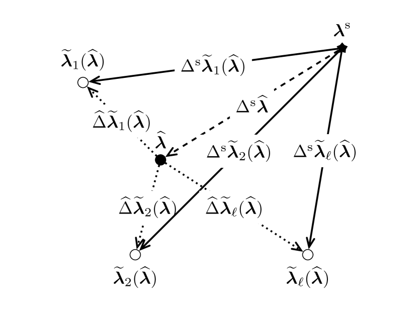
Figure 1: Relationship between the signal parameters 𝝀ssuperscript𝝀s\boldsymbol{\lambda}^{\mathrm{s}}, its nearest semicoherent template 𝝀^^𝝀\widehat{\boldsymbol{\lambda}}, and its N𝑁N nearest coherent templates 𝝀~1,𝝀~2,,𝝀~,subscript~𝝀1subscript~𝝀2subscript~𝝀\widetilde{\boldsymbol{\lambda}}_{1},\widetilde{\boldsymbol{\lambda}}_{2},\dots,\widetilde{\boldsymbol{\lambda}}_{\ell},\dots, following Fig. 1 of Prix and Shaltev (2012).

This section describes a common semicoherent search method for gravitational-wave pulsars, referred to as “interpolating StackSlide” in Prix and Shaltev (2012).

The gravitational-wave detector data are partitioned in time into N𝑁N segments, labeled with the index =1,2,,N12𝑁\ell=1,2,\dots,N. For simplicity we assume that the time-spans of all segments are identical and equal to T~~𝑇\widetilde{T}; the mid-time of each segment is denoted tsubscript𝑡t_{\ell}. In each segment \ell, the coherent \mathcal{F}-statistic 2~(𝝀~)2subscript~subscript~𝝀2\widetilde{\mathcal{F}}_{\ell}(\widetilde{\boldsymbol{\lambda}}_{\ell}) is calculated on a coherent template bank {𝝀~}𝒫subscript~𝝀𝒫\{\widetilde{\boldsymbol{\lambda}}_{\ell}\}\in\mathcal{P} which is constructed using the coherent metric 𝐠~subscript~𝐠\widetilde{\boldsymbol{\mathrm{g}}}_{\ell} at a common reference time t0subscript𝑡0t_{0}. As the metrics 𝐠~subscript~𝐠\widetilde{\boldsymbol{\mathrm{g}}}_{\ell} are generally different for each segment, so too will be the template banks {𝝀~}subscript~𝝀\{\widetilde{\boldsymbol{\lambda}}_{\ell}\}.

The semicoherent \mathcal{F}-statistic is computed on a distinct, semicoherent template bank {𝝀^}𝒫^𝝀𝒫\{\widehat{\boldsymbol{\lambda}}\}\in\mathcal{P}. For each semicoherent template 𝝀^^𝝀\widehat{\boldsymbol{\lambda}}, the coherent template in each segment which is nearest to 𝝀^^𝝀\widehat{\boldsymbol{\lambda}}, as measured by the respective coherent metric 𝐠~subscript~𝐠\widetilde{\boldsymbol{\mathrm{g}}}_{\ell}, is determined; these N𝑁N templates are denoted 𝝀~(𝝀^)subscript~𝝀^𝝀\widetilde{\boldsymbol{\lambda}}_{\ell}(\widehat{\boldsymbol{\lambda}}). The metric mismatch between 𝝀^^𝝀\widehat{\boldsymbol{\lambda}} and 𝝀~(𝝀^)subscript~𝝀^𝝀\widetilde{\boldsymbol{\lambda}}_{\ell}(\widehat{\boldsymbol{\lambda}}) is denoted

μ~(𝝀^;𝝀~(𝝀^))Δ^𝝀~(𝝀^)𝐠~Δ^𝝀~(𝝀^),subscript~𝜇^𝝀subscript~𝝀^𝝀^Δsubscript~𝝀^𝝀subscript~𝐠^Δsubscript~𝝀^𝝀\widetilde{\mu}_{\ell}\big{(}\widehat{\boldsymbol{\lambda}};\widetilde{\boldsymbol{\lambda}}_{\ell}(\widehat{\boldsymbol{\lambda}})\big{)}\equiv\widehat{\Delta}\widetilde{\boldsymbol{\lambda}}_{\ell}(\widehat{\boldsymbol{\lambda}})\cdot\widetilde{\boldsymbol{\mathrm{g}}}_{\ell}\cdot\widehat{\Delta}\widetilde{\boldsymbol{\lambda}}_{\ell}(\widehat{\boldsymbol{\lambda}})\,, (11)

where Δ^𝝀~(𝝀^)𝝀~(𝝀^)𝝀^^Δsubscript~𝝀^𝝀subscript~𝝀^𝝀^𝝀\widehat{\Delta}\widetilde{\boldsymbol{\lambda}}_{\ell}(\widehat{\boldsymbol{\lambda}})\equiv\widetilde{\boldsymbol{\lambda}}_{\ell}(\widehat{\boldsymbol{\lambda}})-\widehat{\boldsymbol{\lambda}}; see Fig. 1. Finally, the N𝑁N coherent \mathcal{F}-statistics computed at the 𝝀~(𝝀^)subscript~𝝀^𝝀\widetilde{\boldsymbol{\lambda}}_{\ell}(\widehat{\boldsymbol{\lambda}}), denoted 2~(𝝀~(𝝀^))2subscript~subscript~𝝀^𝝀2\widetilde{\mathcal{F}}_{\ell}\big{(}\widetilde{\boldsymbol{\lambda}}_{\ell}(\widehat{\boldsymbol{\lambda}})\big{)}, are retrieved and summed to give

2^(𝝀~(𝝀^))=1N2~(𝝀~(𝝀^)).2^subscript~𝝀^𝝀superscriptsubscript1𝑁2subscript~subscript~𝝀^𝝀2\widehat{\mathcal{F}}\big{(}\widetilde{\boldsymbol{\lambda}}_{\ell}(\widehat{\boldsymbol{\lambda}})\big{)}\equiv\sum_{\ell=1}^{N}2\widetilde{\mathcal{F}}_{\ell}\big{(}\widetilde{\boldsymbol{\lambda}}_{\ell}(\widehat{\boldsymbol{\lambda}})\big{)}\,. (12)

In noise, 2^(𝝀~(𝝀^))2^subscript~𝝀^𝝀2\widehat{\mathcal{F}}\big{(}\widetilde{\boldsymbol{\lambda}}_{\ell}(\widehat{\boldsymbol{\lambda}})\big{)} is a central χ2superscript𝜒2\chi^{2} statistic with 4N4𝑁4N degrees of freedom; near a signal, it is a noncentral χ2superscript𝜒2\chi^{2} statistic with 4N4𝑁4N degrees of freedom and noncentrality parameter

ρ^2(𝝀s;𝝀~(𝝀^))=1Nρ~2(𝝀s;𝝀~(𝝀^)),superscript^𝜌2superscript𝝀ssubscript~𝝀^𝝀superscriptsubscript1𝑁superscriptsubscript~𝜌2superscript𝝀ssubscript~𝝀^𝝀\widehat{\rho}^{2}\big{(}\boldsymbol{\lambda}^{\mathrm{s}};\widetilde{\boldsymbol{\lambda}}_{\ell}(\widehat{\boldsymbol{\lambda}})\big{)}\equiv\sum_{\ell=1}^{N}\widetilde{\rho}_{\ell}^{2}\big{(}\boldsymbol{\lambda}^{\mathrm{s}};\widetilde{\boldsymbol{\lambda}}_{\ell}(\widehat{\boldsymbol{\lambda}})\big{)}\,, (13)

where ρ~2(𝝀s;𝝀~(𝝀^))superscriptsubscript~𝜌2superscript𝝀ssubscript~𝝀^𝝀\widetilde{\rho}_{\ell}^{2}\big{(}\boldsymbol{\lambda}^{\mathrm{s}};\widetilde{\boldsymbol{\lambda}}_{\ell}(\widehat{\boldsymbol{\lambda}})\big{)} are the noncentrality parameters of the N𝑁N coherent \mathcal{F}-statistics. (Henceforth we suppress the dependencies on the 𝓐𝓐\boldsymbol{\mathcal{A}}.) By Eq. (1), the signal-to-noise ratio of the semicoherent \mathcal{F}-statistic is therefore

SNR^2(𝝀s;𝝀~(𝝀^))=[4N+ρ^2(𝝀s;𝝀~(𝝀^))][4N][8N]/8=1Nρ^2(𝝀s;𝝀~(𝝀^)).superscript^SNR2superscript𝝀ssubscript~𝝀^𝝀delimited-[]4𝑁superscript^𝜌2superscript𝝀ssubscript~𝝀^𝝀delimited-[]4𝑁delimited-[]8𝑁81𝑁superscript^𝜌2superscript𝝀ssubscript~𝝀^𝝀\begin{split}\widehat{\operatorname{SNR}}^{2}\big{(}\boldsymbol{\lambda}^{\mathrm{s}};\widetilde{\boldsymbol{\lambda}}_{\ell}(\widehat{\boldsymbol{\lambda}})\big{)}&=\frac{\big{[}4N+\widehat{\rho}^{2}\big{(}\boldsymbol{\lambda}^{\mathrm{s}};\widetilde{\boldsymbol{\lambda}}_{\ell}(\widehat{\boldsymbol{\lambda}})\big{)}\big{]}-[4N]}{\sqrt{[8N]/8}}\\ &=\frac{1}{\sqrt{N}}\widehat{\rho}^{2}\big{(}\boldsymbol{\lambda}^{\mathrm{s}};\widetilde{\boldsymbol{\lambda}}_{\ell}(\widehat{\boldsymbol{\lambda}})\big{)}\,.\end{split} (14)

Note that Eq. (14) is a factor of N𝑁\sqrt{N} less than the signal-to-noise ratio of a fully-coherent search using the same amount of data NT~𝑁~𝑇N\widetilde{T}.

The definition of the semicoherent mismatch follows from Eq. (3):

μ^0(𝝀s;𝝀~(𝝀^))superscript^𝜇0superscript𝝀ssubscript~𝝀^𝝀\displaystyle\widehat{\mu}^{0}\big{(}\boldsymbol{\lambda}^{\mathrm{s}};\widetilde{\boldsymbol{\lambda}}_{\ell}(\widehat{\boldsymbol{\lambda}})\big{)} 1SNR^2(𝝀s;𝝀~(𝝀^))SNR^2(𝝀s;𝝀s),absent1superscript^SNR2superscript𝝀ssubscript~𝝀^𝝀superscript^SNR2superscript𝝀ssuperscript𝝀s\displaystyle\equiv 1-\frac{\widehat{\operatorname{SNR}}^{2}\big{(}\boldsymbol{\lambda}^{\mathrm{s}};\widetilde{\boldsymbol{\lambda}}_{\ell}(\widehat{\boldsymbol{\lambda}})\big{)}}{\widehat{\operatorname{SNR}}^{2}(\boldsymbol{\lambda}^{\mathrm{s}};\boldsymbol{\lambda}^{\mathrm{s}})}\,, (15)

where SNR^2(𝝀s;𝝀s)superscript^SNR2superscript𝝀ssuperscript𝝀s\widehat{\operatorname{SNR}}^{2}(\boldsymbol{\lambda}^{\mathrm{s}};\boldsymbol{\lambda}^{\mathrm{s}}) is the signal-to-noise ratio at perfect match in both coherent and semicoherent templates. Substituting Eq. (14) demonstrates that the semicoherent mismatch can equivalently be defined as the loss in noncentrality parameter, c.f. Eq. (18) of Prix and Shaltev (2012):

μ^0(𝝀s;𝝀~(𝝀^))=1ρ^2(𝝀s;𝝀~(𝝀^))ρ^2(𝝀s;𝝀s).superscript^𝜇0superscript𝝀ssubscript~𝝀^𝝀1superscript^𝜌2superscript𝝀ssubscript~𝝀^𝝀superscript^𝜌2superscript𝝀ssuperscript𝝀s\widehat{\mu}^{0}\big{(}\boldsymbol{\lambda}^{\mathrm{s}};\widetilde{\boldsymbol{\lambda}}_{\ell}(\widehat{\boldsymbol{\lambda}})\big{)}=1-\frac{\widehat{\rho}^{2}\big{(}\boldsymbol{\lambda}^{\mathrm{s}};\widetilde{\boldsymbol{\lambda}}_{\ell}(\widehat{\boldsymbol{\lambda}})\big{)}}{\widehat{\rho}^{2}(\boldsymbol{\lambda}^{\mathrm{s}};\boldsymbol{\lambda}^{\mathrm{s}})}\,. (16)

where ρ^2(𝝀s;𝝀s)superscript^𝜌2superscript𝝀ssuperscript𝝀s\widehat{\rho}^{2}(\boldsymbol{\lambda}^{\mathrm{s}};\boldsymbol{\lambda}^{\mathrm{s}}) is the noncentrality parameter at perfect match in both coherent and semicoherent templates. It is assumed that the coherent noncentrality parameter at perfect match is constant over all segments, which implies

ρ^2(𝝀s;𝝀s)Nρ~2(𝝀s;𝝀s).superscript^𝜌2superscript𝝀ssuperscript𝝀s𝑁superscriptsubscript~𝜌2superscript𝝀ssuperscript𝝀s\widehat{\rho}^{2}(\boldsymbol{\lambda}^{\mathrm{s}};\boldsymbol{\lambda}^{\mathrm{s}})\equiv N\widetilde{\rho}_{\ell}^{2}(\boldsymbol{\lambda}^{\mathrm{s}};\boldsymbol{\lambda}^{\mathrm{s}})\,. (17)

Substituting Eqs. (13), and (17) into Eq. (16) yields

μ^0(𝝀s;𝝀~(𝝀^))superscript^𝜇0superscript𝝀ssubscript~𝝀^𝝀\displaystyle\widehat{\mu}^{0}\big{(}\boldsymbol{\lambda}^{\mathrm{s}};\widetilde{\boldsymbol{\lambda}}_{\ell}(\widehat{\boldsymbol{\lambda}})\big{)} =11N=1Nρ~2(𝝀s;𝝀~(𝝀^))ρ~2(𝝀s;𝝀s)absent11𝑁superscriptsubscript1𝑁superscriptsubscript~𝜌2superscript𝝀ssubscript~𝝀^𝝀superscriptsubscript~𝜌2superscript𝝀ssuperscript𝝀s\displaystyle=1-\frac{1}{N}\sum_{\ell=1}^{N}\frac{\widetilde{\rho}_{\ell}^{2}\big{(}\boldsymbol{\lambda}^{\mathrm{s}};\widetilde{\boldsymbol{\lambda}}_{\ell}(\widehat{\boldsymbol{\lambda}})\big{)}}{\widetilde{\rho}_{\ell}^{2}(\boldsymbol{\lambda}^{\mathrm{s}};\boldsymbol{\lambda}^{\mathrm{s}})} (18)
=1N=1Nμ~0(𝝀s;𝝀~(𝝀^)),absent1𝑁superscriptsubscript1𝑁superscriptsubscript~𝜇0superscript𝝀ssubscript~𝝀^𝝀\displaystyle=\frac{1}{N}\sum_{\ell=1}^{N}\widetilde{\mu}_{\ell}^{0}\big{(}\boldsymbol{\lambda}^{\mathrm{s}};\widetilde{\boldsymbol{\lambda}}_{\ell}(\widehat{\boldsymbol{\lambda}})\big{)}\,, (19)

where μ~0(𝝀s;𝝀~(𝝀^))superscriptsubscript~𝜇0superscript𝝀ssubscript~𝝀^𝝀\widetilde{\mu}_{\ell}^{0}\big{(}\boldsymbol{\lambda}^{\mathrm{s}};\widetilde{\boldsymbol{\lambda}}_{\ell}(\widehat{\boldsymbol{\lambda}})\big{)} is the coherent mismatch in the \ellth segment between the nearest template 𝝀~(𝝀^)subscript~𝝀^𝝀\widetilde{\boldsymbol{\lambda}}_{\ell}(\widehat{\boldsymbol{\lambda}}) and the signal 𝝀ssuperscript𝝀s\boldsymbol{\lambda}^{\mathrm{s}}. Further substitution of Eq. (7) results in

μ^0(𝝀s;𝝀~(𝝀^))1N=1NΔs𝝀~(𝝀^)𝐠~ϕ(𝝀s)Δs𝝀~(𝝀^),superscript^𝜇0superscript𝝀ssubscript~𝝀^𝝀1𝑁superscriptsubscript1𝑁superscriptΔssubscript~𝝀^𝝀superscriptsubscript~𝐠italic-ϕsuperscript𝝀ssuperscriptΔssubscript~𝝀^𝝀\widehat{\mu}^{0}\big{(}\boldsymbol{\lambda}^{\mathrm{s}};\widetilde{\boldsymbol{\lambda}}_{\ell}(\widehat{\boldsymbol{\lambda}})\big{)}\approx\frac{1}{N}\sum_{\ell=1}^{N}\Delta^{\mathrm{s}}\widetilde{\boldsymbol{\lambda}}_{\ell}(\widehat{\boldsymbol{\lambda}})\cdot\widetilde{\boldsymbol{\mathrm{g}}}_{\ell}^{\phi}(\boldsymbol{\lambda}^{\mathrm{s}})\cdot\Delta^{\mathrm{s}}\widetilde{\boldsymbol{\lambda}}_{\ell}(\widehat{\boldsymbol{\lambda}})\,, (20)

where (see Fig. 1)

Δs𝝀~(𝝀^)superscriptΔssubscript~𝝀^𝝀\displaystyle\Delta^{\mathrm{s}}\widetilde{\boldsymbol{\lambda}}_{\ell}(\widehat{\boldsymbol{\lambda}}) 𝝀~(𝝀^)𝝀sabsentsubscript~𝝀^𝝀superscript𝝀s\displaystyle\equiv\widetilde{\boldsymbol{\lambda}}_{\ell}(\widehat{\boldsymbol{\lambda}})-\boldsymbol{\lambda}^{\mathrm{s}} (21)
=(𝝀~(𝝀^)𝝀^)+(𝝀^𝝀s)absentsubscript~𝝀^𝝀^𝝀^𝝀superscript𝝀s\displaystyle=\big{(}\widetilde{\boldsymbol{\lambda}}_{\ell}(\widehat{\boldsymbol{\lambda}})-\widehat{\boldsymbol{\lambda}}\big{)}+\big{(}\widehat{\boldsymbol{\lambda}}-\boldsymbol{\lambda}^{\mathrm{s}}\big{)} (22)
=Δ^𝝀~(𝝀^)+Δs𝝀^.absent^Δsubscript~𝝀^𝝀superscriptΔs^𝝀\displaystyle=\widehat{\Delta}\widetilde{\boldsymbol{\lambda}}_{\ell}(\widehat{\boldsymbol{\lambda}})+\Delta^{\mathrm{s}}\widehat{\boldsymbol{\lambda}}\,. (23)

Finally, substituting Eq. (23) into Eq. (20) gives

μ^0(𝝀s;𝝀~(𝝀^))1N=1NΔs𝝀^𝐠~ϕ(𝝀s)Δs𝝀^+1N=1NΔ^𝝀~(𝝀^)𝐠~ϕ(𝝀s)Δ^𝝀~(𝝀^)+2N=1NΔ^𝝀~(𝝀^)𝐠~ϕ(𝝀s)Δs𝝀^.superscript^𝜇0superscript𝝀ssubscript~𝝀^𝝀1𝑁superscriptsubscript1𝑁superscriptΔs^𝝀superscriptsubscript~𝐠italic-ϕsuperscript𝝀ssuperscriptΔs^𝝀1𝑁superscriptsubscript1𝑁^Δsubscript~𝝀^𝝀superscriptsubscript~𝐠italic-ϕsuperscript𝝀s^Δsubscript~𝝀^𝝀2𝑁superscriptsubscript1𝑁^Δsubscript~𝝀^𝝀superscriptsubscript~𝐠italic-ϕsuperscript𝝀ssuperscriptΔs^𝝀\begin{split}\widehat{\mu}^{0}\big{(}\boldsymbol{\lambda}^{\mathrm{s}};\widetilde{\boldsymbol{\lambda}}_{\ell}(\widehat{\boldsymbol{\lambda}})\big{)}&\approx\frac{1}{N}\sum_{\ell=1}^{N}\Delta^{\mathrm{s}}\widehat{\boldsymbol{\lambda}}\cdot\widetilde{\boldsymbol{\mathrm{g}}}_{\ell}^{\phi}(\boldsymbol{\lambda}^{\mathrm{s}})\cdot\Delta^{\mathrm{s}}\widehat{\boldsymbol{\lambda}}\\ &+\frac{1}{N}\sum_{\ell=1}^{N}\widehat{\Delta}\widetilde{\boldsymbol{\lambda}}_{\ell}(\widehat{\boldsymbol{\lambda}})\cdot\widetilde{\boldsymbol{\mathrm{g}}}_{\ell}^{\phi}(\boldsymbol{\lambda}^{\mathrm{s}})\cdot\widehat{\Delta}\widetilde{\boldsymbol{\lambda}}_{\ell}(\widehat{\boldsymbol{\lambda}})\\ &+\frac{2}{N}\sum_{\ell=1}^{N}\widehat{\Delta}\widetilde{\boldsymbol{\lambda}}_{\ell}(\widehat{\boldsymbol{\lambda}})\cdot\widetilde{\boldsymbol{\mathrm{g}}}_{\ell}^{\phi}(\boldsymbol{\lambda}^{\mathrm{s}})\cdot\Delta^{\mathrm{s}}\widehat{\boldsymbol{\lambda}}\,.\end{split} (24)

The first term on the right-hand side of Eq. (24) is the mismatch between the signal 𝝀ssuperscript𝝀s\boldsymbol{\lambda}^{\mathrm{s}} and the semicoherent template 𝝀^^𝝀\widehat{\boldsymbol{\lambda}} in the ideal case of no interpolation, i.e. supposing Δ^𝝀~(𝝀^)=0^Δsubscript~𝝀^𝝀0\widehat{\Delta}\widetilde{\boldsymbol{\lambda}}_{\ell}(\widehat{\boldsymbol{\lambda}})=0 for all \ell. It may be written as

μ^ni0(𝝀s;𝝀^)subscriptsuperscript^𝜇0nisuperscript𝝀s^𝝀\displaystyle\widehat{\mu}^{0}_{\textrm{ni}}(\boldsymbol{\lambda}^{\mathrm{s}};\widehat{\boldsymbol{\lambda}}) 1N=1Nμ~0(𝝀s;𝝀^)absent1𝑁superscriptsubscript1𝑁superscriptsubscript~𝜇0superscript𝝀s^𝝀\displaystyle\equiv\frac{1}{N}\sum_{\ell=1}^{N}\widetilde{\mu}_{\ell}^{0}(\boldsymbol{\lambda}^{\mathrm{s}};\widehat{\boldsymbol{\lambda}}) (25)
1N=1NΔs𝝀^𝐠~ϕ(𝝀s)Δs𝝀^absent1𝑁superscriptsubscript1𝑁superscriptΔs^𝝀superscriptsubscript~𝐠italic-ϕsuperscript𝝀ssuperscriptΔs^𝝀\displaystyle\approx\frac{1}{N}\sum_{\ell=1}^{N}\Delta^{\mathrm{s}}\widehat{\boldsymbol{\lambda}}\cdot\widetilde{\boldsymbol{\mathrm{g}}}_{\ell}^{\phi}(\boldsymbol{\lambda}^{\mathrm{s}})\cdot\Delta^{\mathrm{s}}\widehat{\boldsymbol{\lambda}} (26)
Δs𝝀^𝐠^ϕ(𝝀s)Δs𝝀^,absentsuperscriptΔs^𝝀superscript^𝐠italic-ϕsuperscript𝝀ssuperscriptΔs^𝝀\displaystyle\approx\Delta^{\mathrm{s}}\widehat{\boldsymbol{\lambda}}\cdot\widehat{\boldsymbol{\mathrm{g}}}^{\phi}(\boldsymbol{\lambda}^{\mathrm{s}})\cdot\Delta^{\mathrm{s}}\widehat{\boldsymbol{\lambda}}\,, (27)

where

𝐠^ϕ(𝝀s)1N=1N𝐠~ϕ(𝝀s)superscript^𝐠italic-ϕsuperscript𝝀s1𝑁superscriptsubscript1𝑁superscriptsubscript~𝐠italic-ϕsuperscript𝝀s\widehat{\boldsymbol{\mathrm{g}}}^{\phi}(\boldsymbol{\lambda}^{\mathrm{s}})\equiv\frac{1}{N}\sum_{\ell=1}^{N}\widetilde{\boldsymbol{\mathrm{g}}}_{\ell}^{\phi}(\boldsymbol{\lambda}^{\mathrm{s}}) (28)

is the semicoherent parameter-space metric; cf. Eq. (2.9) of Brady and Creighton (2000). The second term on the right-hand side of Eq. (24) is the mismatch purely from interpolation,

μ^pi0(𝝀^;𝝀~(𝝀^))subscriptsuperscript^𝜇0pi^𝝀subscript~𝝀^𝝀\displaystyle\widehat{\mu}^{0}_{\textrm{pi}}\big{(}\widehat{\boldsymbol{\lambda}};\widetilde{\boldsymbol{\lambda}}_{\ell}(\widehat{\boldsymbol{\lambda}})\big{)} 1N=1Nμ~0(𝝀^;𝝀~(𝝀^))absent1𝑁superscriptsubscript1𝑁superscriptsubscript~𝜇0^𝝀subscript~𝝀^𝝀\displaystyle\equiv\frac{1}{N}\sum_{\ell=1}^{N}\widetilde{\mu}_{\ell}^{0}\big{(}\widehat{\boldsymbol{\lambda}};\widetilde{\boldsymbol{\lambda}}_{\ell}(\widehat{\boldsymbol{\lambda}})\big{)} (29)
1N=1NΔ^𝝀~(𝝀^)𝐠~ϕ(𝝀s)Δ^𝝀~(𝝀^).absent1𝑁superscriptsubscript1𝑁^Δsubscript~𝝀^𝝀superscriptsubscript~𝐠italic-ϕsuperscript𝝀s^Δsubscript~𝝀^𝝀\displaystyle\approx\frac{1}{N}\sum_{\ell=1}^{N}\widehat{\Delta}\widetilde{\boldsymbol{\lambda}}_{\ell}(\widehat{\boldsymbol{\lambda}})\cdot\widetilde{\boldsymbol{\mathrm{g}}}_{\ell}^{\phi}(\boldsymbol{\lambda}^{\mathrm{s}})\cdot\widehat{\Delta}\widetilde{\boldsymbol{\lambda}}_{\ell}(\widehat{\boldsymbol{\lambda}})\,. (30)

The average of the third term on the right-hand side of Eq. (24) will tend to zero when N𝑁N is large, and when μ^ni0subscriptsuperscript^𝜇0ni\widehat{\mu}^{0}_{\textrm{ni}} is averaged over many different signals 𝝀ssuperscript𝝀s\boldsymbol{\lambda}^{\mathrm{s}} Prix and Shaltev (2012). This is because the term is linear in the offsets Δ^𝝀~(𝝀^)^Δsubscript~𝝀^𝝀\widehat{\Delta}\widetilde{\boldsymbol{\lambda}}_{\ell}(\widehat{\boldsymbol{\lambda}}) and Δs𝝀^superscriptΔs^𝝀\Delta^{\mathrm{s}}\widehat{\boldsymbol{\lambda}}, which are presumed to be equally distributed about zero. Likewise, under the same conditions the average of Eq. (29) will tend to μ~0delimited-⟨⟩superscriptsubscript~𝜇0\langle\widetilde{\mu}_{\ell}^{0}\rangle, the average coherent mismatch. The average of Eq. (15) will therefore tend to

μ^0μ^ni0+μ~0.delimited-⟨⟩superscript^𝜇0delimited-⟨⟩subscriptsuperscript^𝜇0nidelimited-⟨⟩superscriptsubscript~𝜇0\langle\widehat{\mu}^{0}\rangle\rightarrow\langle\widehat{\mu}^{0}_{\textrm{ni}}\rangle+\langle\widetilde{\mu}_{\ell}^{0}\rangle\,. (31)

It follows from Eqs. (31) and (25) that the average semicoherent mismatch μ^0delimited-⟨⟩superscript^𝜇0\langle\widehat{\mu}^{0}\rangle is minimized if 𝝀^{𝝀^}^𝝀^𝝀\widehat{\boldsymbol{\lambda}}\in\{\widehat{\boldsymbol{\lambda}}\} is chosen to be nearest to the signal 𝝀ssuperscript𝝀s\boldsymbol{\lambda}^{\mathrm{s}}, as measured by the semicoherent metric 𝐠^ϕsuperscript^𝐠italic-ϕ\widehat{\boldsymbol{\mathrm{g}}}^{\phi}, thus minimizing μ^ni0delimited-⟨⟩subscriptsuperscript^𝜇0ni\langle\widehat{\mu}^{0}_{\textrm{ni}}\rangle.

Therefore, the semicoherent template bank {𝝀^}^𝝀\{\widehat{\boldsymbol{\lambda}}\} should be constructed similarly to the coherent template banks {𝝀~}subscript~𝝀\{\widetilde{\boldsymbol{\lambda}}_{\ell}\}, using 𝐠^ϕsuperscript^𝐠italic-ϕ\widehat{\boldsymbol{\mathrm{g}}}^{\phi} to minimize μ^ni0subscriptsuperscript^𝜇0ni\widehat{\mu}^{0}_{\textrm{ni}}, and hence μ^0delimited-⟨⟩superscript^𝜇0\langle\widehat{\mu}^{0}\rangle, at fixed number of semicoherent templates 𝒩^|{𝝀^}|^𝒩^𝝀\widehat{\mathcal{N}}\equiv|\{\widehat{\boldsymbol{\lambda}}\}|. This may be achieved using lattice template placement (see Paper II), but only if 𝐠^ϕsuperscript^𝐠italic-ϕ\widehat{\boldsymbol{\mathrm{g}}}^{\phi} is constant with respect to 𝓐𝓐\boldsymbol{\mathcal{A}} and 𝝀ssuperscript𝝀s\boldsymbol{\lambda}^{\mathrm{s}}. The construction of such a metric, starting from the semicoherent phase metric 𝐠^ϕ(𝝀s)=1N𝐠~ϕ(𝝀s)/Nsuperscript^𝐠italic-ϕsuperscript𝝀ssuperscriptsubscript1𝑁superscriptsubscript~𝐠italic-ϕsuperscript𝝀s𝑁\widehat{\boldsymbol{\mathrm{g}}}^{\phi}(\boldsymbol{\lambda}^{\mathrm{s}})\equiv\sum_{\ell=1}^{N}\widetilde{\boldsymbol{\mathrm{g}}}_{\ell}^{\phi}(\boldsymbol{\lambda}^{\mathrm{s}})/N, is the subject of the next section.

III Semicoherent supersky parameter-space metric

This section introduces a close approximation to 𝐠^ϕ(𝝀s)superscript^𝐠italic-ϕsuperscript𝝀s\widehat{\boldsymbol{\mathrm{g}}}^{\phi}(\boldsymbol{\lambda}^{\mathrm{s}}) which is constant with respect to all phase parameters λ𝜆\lambda: the semicoherent reduced supersky metric 𝐠^^𝐠\widehat{\boldsymbol{\mathrm{g}}}. Its derivation, presented in Section III.1, closely follows that of the coherent metric 𝐠~subscript~𝐠\widetilde{\boldsymbol{\mathrm{g}}}_{\ell}, which is described in Section II.2 and Paper I. The new metric is validated using numerical simulations presented in Section III.2.

III.1 Derivation

Refer to caption
(a)
Refer to caption
(b)
Refer to caption
(c)
Refer to caption
(d)
Refer to caption
(e)
Refer to caption
(f)
Refer to caption
(g)
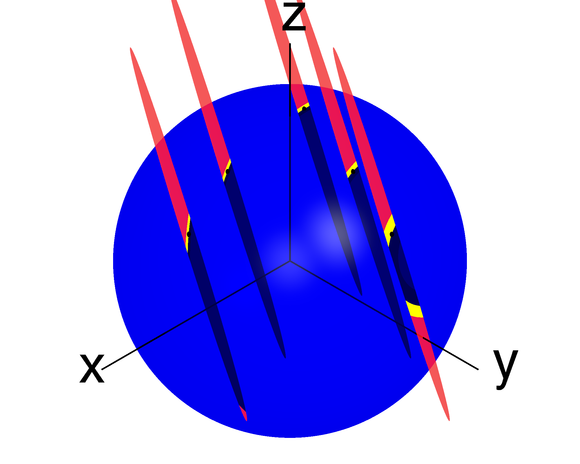
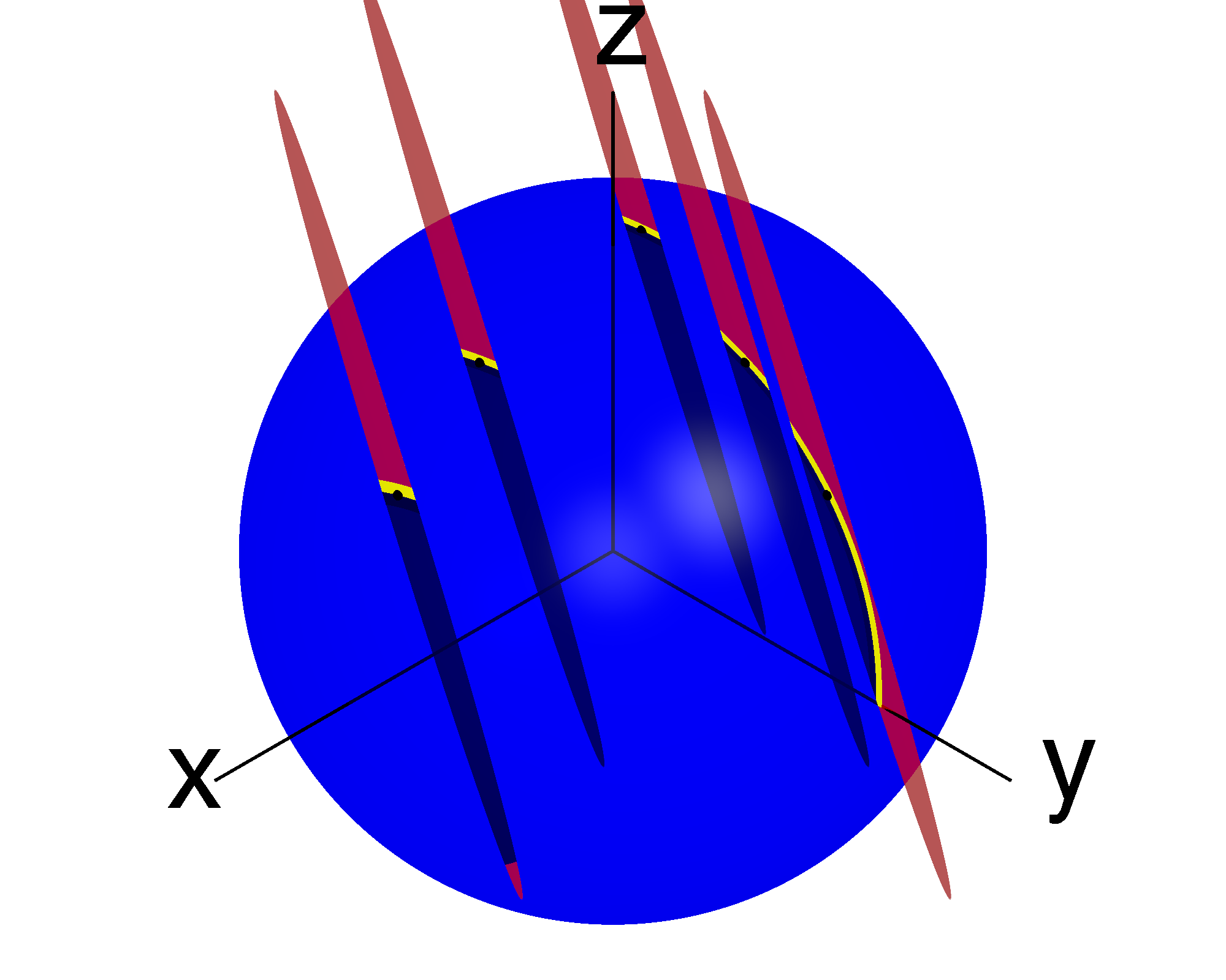
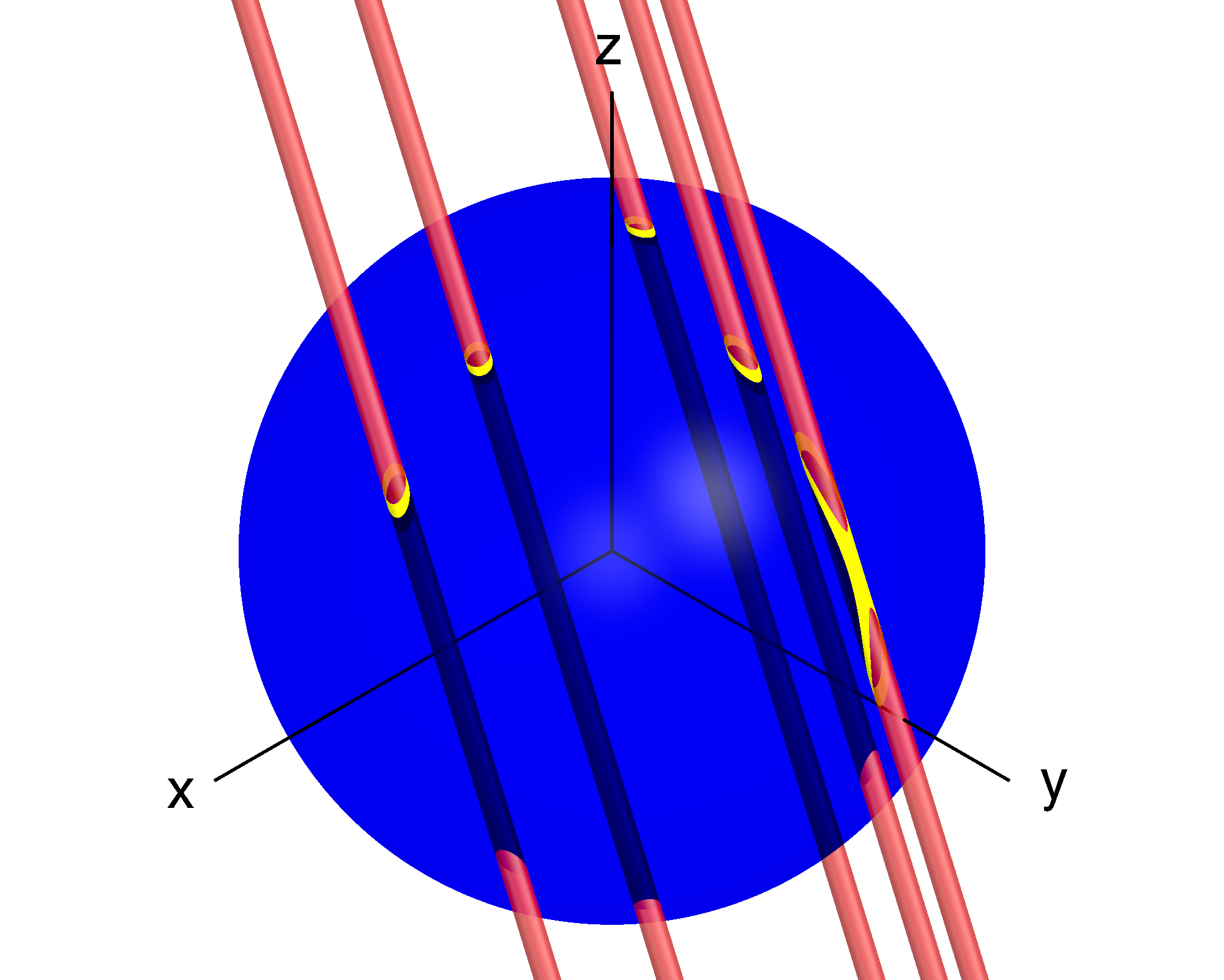
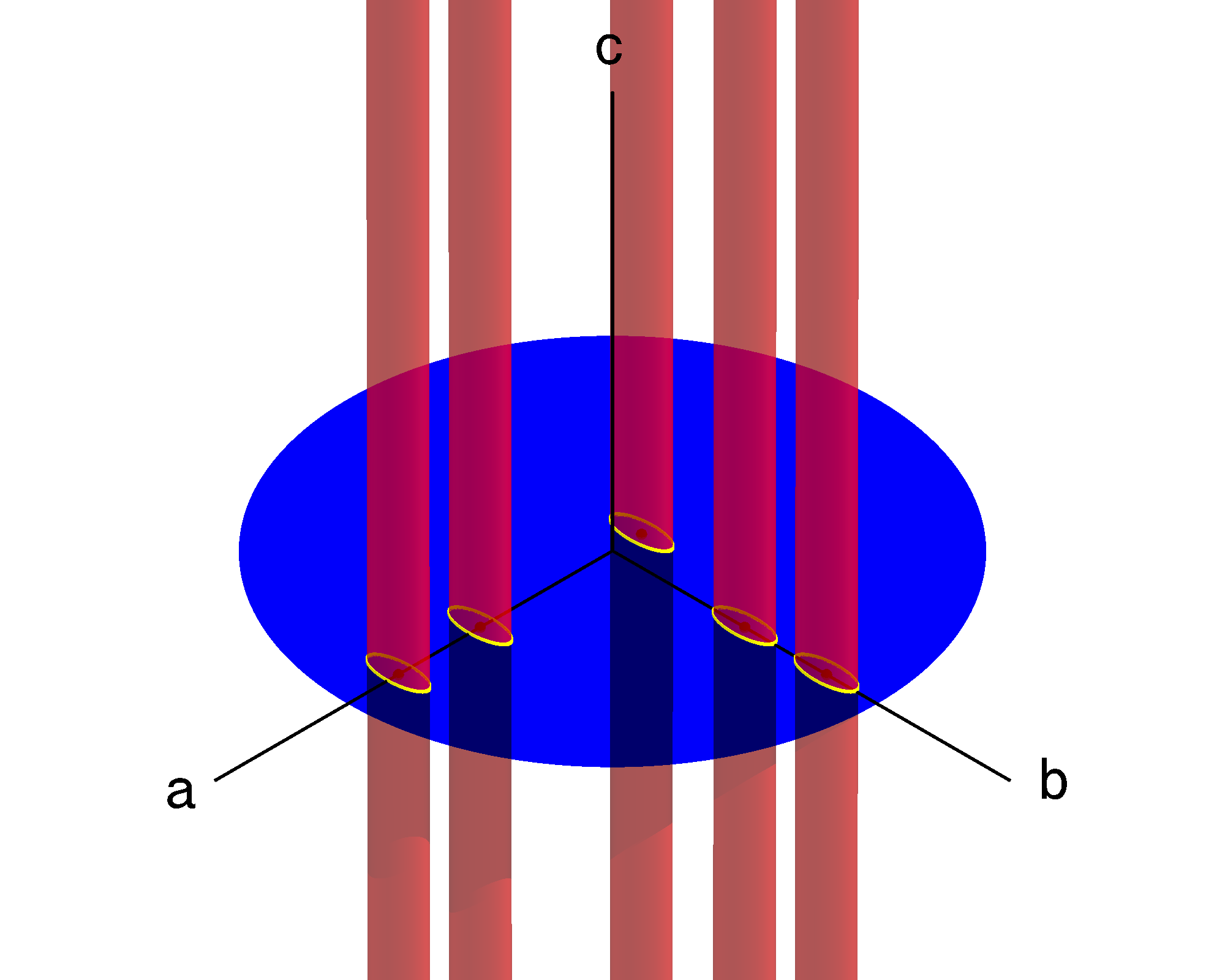
Figure 2: Metric ellipsoids of the coherent and semicoherent supersky metrics, at 5 example sky points. LABEL:sub@fig:seg1_ssky_ellipsesLABEL:sub@fig:seg5_ssky_ellipses: Metric ellipsoids (red) of 5 coherent unconstrained supersky metrics 𝐠~usuperscriptsubscript~𝐠u\widetilde{\boldsymbol{\mathrm{g}}}_{\ell}^{\textrm{u}}, in equatorial coordinates (x,y,z)𝑥𝑦𝑧(x,y,z), for μ~max=30subscript~𝜇max30\widetilde{\mu}_{\textrm{max}}=30, T~=4~𝑇4\widetilde{T}=4 days, fmax=1subscript𝑓max1f_{\textrm{max}}=1 kHz, t0=UTC 2015-01-01 00:00:00subscript𝑡0UTC 2015-01-01 00:00:00t_{0}=\text{UTC 2015-01-01 00:00:00}, and tt0=180,90,0,+90,+180subscript𝑡subscript𝑡018090090180t_{\ell}-t_{0}=-180,-90,0,+90,+180 days respectively. Their intersection with the sky sphere |𝒏|=1𝒏1|\boldsymbol{n}|=1 (blue) reproduces the coherent physical sky metric (yellow). LABEL:sub@fig:avg_ssky_ellipses: Metric ellipsoids (red) of the semicoherent unconstrained supersky metric 𝐠^u==15𝐠~u/5superscript^𝐠usuperscriptsubscript15superscriptsubscript~𝐠u5\widehat{\boldsymbol{\mathrm{g}}}^{\textrm{u}}=\sum_{\ell=1}^{5}\widetilde{\boldsymbol{\mathrm{g}}}_{\ell}^{\textrm{u}}/5, for μ^max=1500subscript^𝜇max1500\widehat{\mu}_{\textrm{max}}=1500. Its intersection with the sky sphere (blue) reproduces the semicoherent physical sky metric (yellow). LABEL:sub@fig:avg_aligned_ssky_ellipses: Metric ellipsoids (red) of the transformed metric 𝒯𝐠^u𝒯superscript^𝐠u\cal T\widehat{\boldsymbol{\mathrm{g}}}^{\textrm{u}}, in coordinates (a,b,c)𝑎𝑏𝑐(a,b,c) given by its sky eigenvectors, for μ^max=1500subscript^𝜇max1500\widehat{\mu}_{\textrm{max}}=1500. Its projection onto the disk c=0𝑐0c=0 (blue) generates the semicoherent supersky metric 𝐠^=𝒥𝒯𝐠^u^𝐠𝒥𝒯superscript^𝐠u\widehat{\boldsymbol{\mathrm{g}}}=\mathcal{J}\mathcal{T}\widehat{\boldsymbol{\mathrm{g}}}^{\textrm{u}} in (n^a,n^b)subscript^𝑛𝑎subscript^𝑛𝑏(\widehat{n}_{a},\widehat{n}_{b}) coordinates (yellow).

First, 𝐠~ϕ(𝝀s)superscriptsubscript~𝐠italic-ϕsuperscript𝝀s\widetilde{\boldsymbol{\mathrm{g}}}_{\ell}^{\phi}(\boldsymbol{\lambda}^{\mathrm{s}}) are computed for all segments, at a common reference time t0subscript𝑡0t_{0}, using the components of 𝒏𝒏\boldsymbol{n} as sky coordinates; these metrics are the coherent unconstrained supersky metrics 𝐠~usuperscriptsubscript~𝐠u\widetilde{\boldsymbol{\mathrm{g}}}_{\ell}^{\textrm{u}}. Second, the 𝐠~usuperscriptsubscript~𝐠u\widetilde{\boldsymbol{\mathrm{g}}}_{\ell}^{\textrm{u}} are averaged to give 𝐠^u=1N𝐠~u/Nsuperscript^𝐠usuperscriptsubscript1𝑁superscriptsubscript~𝐠u𝑁\widehat{\boldsymbol{\mathrm{g}}}^{\textrm{u}}\equiv\sum_{\ell=1}^{N}\widetilde{\boldsymbol{\mathrm{g}}}_{\ell}^{\textrm{u}}/N, the semicoherent unconstrained supersky metric. Finally, the procedure described in Section II.2 and Paper I, denoted by the operators 𝒥𝒯𝒥𝒯\mathcal{J}\mathcal{T}, is applied to 𝐠^usuperscript^𝐠u\widehat{\boldsymbol{\mathrm{g}}}^{\textrm{u}} to give the semicoherent supersky metric

𝐠^𝒥𝒯N[=1N𝐠~u].^𝐠𝒥𝒯𝑁delimited-[]superscriptsubscript1𝑁superscriptsubscript~𝐠u\widehat{\boldsymbol{\mathrm{g}}}\equiv\frac{\mathcal{J}\mathcal{T}}{N}\left[\sum_{\ell=1}^{N}\widetilde{\boldsymbol{\mathrm{g}}}_{\ell}^{\textrm{u}}\right]\,. (32)

The phase parameters associated with 𝐠^^𝐠\widehat{\boldsymbol{\mathrm{g}}} are the sky parameters (n^a,n^b)subscript^𝑛𝑎subscript^𝑛𝑏(\widehat{n}_{a},\widehat{n}_{b}), and the frequency/spindowns ν^(s)f(s)+𝚫𝒔^𝒏superscript^𝜈𝑠superscript𝑓𝑠^superscript𝚫𝒔𝒏\widehat{\nu}^{(s)}\equiv f^{(s)}+\widehat{\boldsymbol{\Delta^{s}}}\cdot\boldsymbol{n}, where the 𝚫𝒔^^superscript𝚫𝒔\widehat{\boldsymbol{\Delta^{s}}} are vectors computed when applying 𝒯𝒯\mathcal{T}.

Figure 2 illustrates this process using an example setup of N=5𝑁5N=5 segments, each spanning T~=4~𝑇4\widetilde{T}=4 days, with segment mid-times tsubscript𝑡t_{\ell} distributed evenly over a total time-span T^=364^𝑇364\widehat{T}=364 days. The effect of the changing segment mid-time on the metrics 𝐠~usuperscriptsubscript~𝐠u\widetilde{\boldsymbol{\mathrm{g}}}_{\ell}^{\textrm{u}} is to rotate their metric ellipsoids (i.e. the volumes that satisfy Δs𝝀~𝐠~uΔs𝝀~μ~maxsuperscriptΔssubscript~𝝀superscriptsubscript~𝐠usuperscriptΔssubscript~𝝀subscript~𝜇max\Delta^{\mathrm{s}}\widetilde{\boldsymbol{\lambda}}_{\ell}\cdot\widetilde{\boldsymbol{\mathrm{g}}}_{\ell}^{\textrm{u}}\cdot\Delta^{\mathrm{s}}\widetilde{\boldsymbol{\lambda}}_{\ell}\leq\widetilde{\mu}_{\textrm{max}} for some μ~maxsubscript~𝜇max\widetilde{\mu}_{\textrm{max}}) around their longest axis, as may be discerned from Figs. 2a2e. The metric ellipsoid of the semicoherent metric 𝐠^usuperscript^𝐠u\widehat{\boldsymbol{\mathrm{g}}}^{\textrm{u}}, in this case, retains the same orientation of the longest axis as the coherent metrics, and still results in a non-constant physical metric (Fig. 2f). Applying 𝒯𝒯\mathcal{T} to 𝐠^usuperscript^𝐠u\widehat{\boldsymbol{\mathrm{g}}}^{\textrm{u}}, however, reorients the metric ellipsoids along the c𝑐c axis (Fig. 2g), corresponding to the eigenvector of the 3×3333\times 3 sky block of 𝐠^usuperscript^𝐠u\widehat{\boldsymbol{\mathrm{g}}}^{\textrm{u}} with the smallest eigenvalue. Applying 𝒥𝒥\mathcal{J} then projects 𝒯𝐠^u𝒯superscript^𝐠u\mathcal{T}\widehat{\boldsymbol{\mathrm{g}}}^{\textrm{u}} onto the disk c=0𝑐0c=0, giving the metric 𝐠^^𝐠\widehat{\boldsymbol{\mathrm{g}}}.

Note that, contrary to Eq. (28), 𝐠^^𝐠\widehat{\boldsymbol{\mathrm{g}}} is not a simple average of the metrics 𝐠~subscript~𝐠\widetilde{\boldsymbol{\mathrm{g}}}_{\ell}, i.e.

𝒥𝒯N[=1N𝐠~u]=𝐠^1N=1N𝐠~==1N𝒥𝒯[𝐠~u]N.𝒥𝒯𝑁delimited-[]superscriptsubscript1𝑁superscriptsubscript~𝐠u^𝐠1𝑁superscriptsubscript1𝑁subscript~𝐠superscriptsubscript1𝑁𝒥𝒯delimited-[]superscriptsubscript~𝐠u𝑁\frac{\mathcal{J}\mathcal{T}}{N}\left[\sum_{\ell=1}^{N}\widetilde{\boldsymbol{\mathrm{g}}}_{\ell}^{\textrm{u}}\right]=\widehat{\boldsymbol{\mathrm{g}}}\neq\frac{1}{N}\sum_{\ell=1}^{N}\widetilde{\boldsymbol{\mathrm{g}}}_{\ell}=\sum_{\ell=1}^{N}\frac{\mathcal{J}\mathcal{T}\big{[}\widetilde{\boldsymbol{\mathrm{g}}}_{\ell}^{\textrm{u}}\big{]}}{N}\,. (33)

There are two reasons why Eq. (33) does not hold. First, Eqs. (27) and (28) hold only if the Δs𝝀^superscriptΔs^𝝀\Delta^{\mathrm{s}}\widehat{\boldsymbol{\lambda}}, and hence the 𝐠~subscript~𝐠\widetilde{\boldsymbol{\mathrm{g}}}_{\ell}, are expressed in a common coordinate system; each 𝐠~subscript~𝐠\widetilde{\boldsymbol{\mathrm{g}}}_{\ell}, however, is expressed in a per-segment coordinate system (na~,nb~,ν~(s))subscript~subscript𝑛𝑎subscript~subscript𝑛𝑏superscriptsubscript~𝜈𝑠(\widetilde{n_{a}}_{\ell},\widetilde{n_{b}}_{\ell},\widetilde{\nu}_{\ell}^{(s)}). Second, the operator 𝒥𝒥\mathcal{J} in general projects each 𝒯𝐠~u𝒯superscriptsubscript~𝐠u\mathcal{T}\widetilde{\boldsymbol{\mathrm{g}}}_{\ell}^{\textrm{u}} onto distinct hyperplanes in the coordinate space of 𝒏𝒏\boldsymbol{n}, and is therefore a nonlinear operator which does not commute with the averaging in Eq. (28).

III.2 Validation using numerical simulations

The ability of the semicoherent supersky metric 𝐠^^𝐠\widehat{\boldsymbol{\mathrm{g}}} to predict the \mathcal{F}-statistic mismatch μ^0superscript^𝜇0\widehat{\mu}^{0} is characterized using numerical simulations, the results of which are presented in this section.

III.2.1 Simulation procedure

T~~𝑇\widetilde{T} / days
1 3 5 7
N𝑁N T^^𝑇\widehat{T}/d η𝜂\eta Sni0subscriptsuperscript𝑆0niS^{0}_{\textrm{ni}} S0superscript𝑆0S^{0} Sni.5subscriptsuperscript𝑆.5niS^{.5}_{\textrm{ni}} S.5superscript𝑆.5S^{.5} T^^𝑇\widehat{T}/d η𝜂\eta Sni0subscriptsuperscript𝑆0niS^{0}_{\textrm{ni}} S0superscript𝑆0S^{0} Sni.5subscriptsuperscript𝑆.5niS^{.5}_{\textrm{ni}} S.5superscript𝑆.5S^{.5} T^^𝑇\widehat{T}/d η𝜂\eta Sni0subscriptsuperscript𝑆0niS^{0}_{\textrm{ni}} S0superscript𝑆0S^{0} Sni.5subscriptsuperscript𝑆.5niS^{.5}_{\textrm{ni}} S.5superscript𝑆.5S^{.5} T^^𝑇\widehat{T}/d η𝜂\eta Sni0subscriptsuperscript𝑆0niS^{0}_{\textrm{ni}} S0superscript𝑆0S^{0} Sni.5subscriptsuperscript𝑆.5niS^{.5}_{\textrm{ni}} S.5superscript𝑆.5S^{.5}
3 3 1.00 0.90.90.9 1.21.21.2 2.42.42.4 2.82.82.8 9 1.00 1.11.11.1 1.81.81.8 3.13.13.1 \infty 15 1.00 1.01.01.0 2.02.02.0 2.52.52.5 \infty 21 1.00 1.01.01.0 1.91.91.9 1.91.91.9 4.94.94.9
5 5 1.00 0.90.90.9 1.31.31.3 2.42.42.4 3.13.13.1 15 1.00 1.11.11.1 2.12.12.1 2.72.72.7 \infty 25 1.00 1.01.01.0 2.32.32.3 1.81.81.8 \infty 35 1.00 0.80.80.8 2.22.22.2 1.31.31.3 6.06.06.0
7 7 1.00 0.90.90.9 1.31.31.3 2.42.42.4 3.43.43.4 21 1.00 1.11.11.1 2.32.32.3 2.52.52.5 \infty 35 1.00 0.80.80.8 2.62.62.6 1.41.41.4 \infty 49 1.00 0.90.90.9 2.42.42.4 1.51.51.5 5.75.75.7
9 9 1.00 0.90.90.9 1.31.31.3 2.42.42.4 3.53.53.5 27 1.00 1.01.01.0 2.42.42.4 2.02.02.0 \infty 45 1.00 0.80.80.8 2.82.82.8 1.41.41.4 \infty 63 1.00 1.21.21.2 2.52.52.5 1.91.91.9 \infty
11 11 1.00 0.90.90.9 1.31.31.3 2.42.42.4 3.63.63.6 33 1.00 0.90.90.9 2.62.62.6 1.71.71.7 \infty 55 1.00 1.01.01.0 3.03.03.0 1.61.61.6 \infty 77 1.00 1.41.41.4 2.52.52.5 2.22.22.2 \infty
13 13 1.00 0.90.90.9 1.41.41.4 2.42.42.4 3.73.73.7 39 1.00 0.90.90.9 2.72.72.7 1.51.51.5 \infty 65 1.00 1.21.21.2 3.13.13.1 1.91.91.9 \infty 91 1.00 1.61.61.6 2.52.52.5 2.52.52.5 \infty
15 15 1.00 0.90.90.9 1.41.41.4 2.42.42.4 3.93.93.9 45 1.00 0.80.80.8 2.82.82.8 1.41.41.4 \infty 75 1.00 1.31.31.3 3.23.23.2 2.12.12.1 \infty 105 1.00 1.71.71.7 2.52.52.5 2.72.72.7 \infty
17 17 1.00 0.90.90.9 1.41.41.4 2.32.32.3 3.93.93.9 51 1.00 0.90.90.9 2.92.92.9 1.41.41.4 \infty 85 1.00 1.41.41.4 3.43.43.4 2.32.32.3 \infty 119 1.00 1.81.81.8 2.52.52.5 3.03.03.0 \infty
19 19 1.00 0.90.90.9 1.41.41.4 2.32.32.3 3.93.93.9 57 1.00 0.90.90.9 3.03.03.0 1.51.51.5 \infty 95 1.00 1.51.51.5 3.43.43.4 2.52.52.5 \infty 133 1.00 1.81.81.8 2.42.42.4 3.23.23.2 \infty
T^^𝑇\widehat{T}/d N𝑁N η𝜂\eta Sni0subscriptsuperscript𝑆0niS^{0}_{\textrm{ni}} S0superscript𝑆0S^{0} Sni.5subscriptsuperscript𝑆.5niS^{.5}_{\textrm{ni}} S.5superscript𝑆.5S^{.5} N𝑁N η𝜂\eta Sni0subscriptsuperscript𝑆0niS^{0}_{\textrm{ni}} S0superscript𝑆0S^{0} Sni.5subscriptsuperscript𝑆.5niS^{.5}_{\textrm{ni}} S.5superscript𝑆.5S^{.5} N𝑁N η𝜂\eta Sni0subscriptsuperscript𝑆0niS^{0}_{\textrm{ni}} S0superscript𝑆0S^{0} Sni.5subscriptsuperscript𝑆.5niS^{.5}_{\textrm{ni}} S.5superscript𝑆.5S^{.5} N𝑁N η𝜂\eta Sni0subscriptsuperscript𝑆0niS^{0}_{\textrm{ni}} S0superscript𝑆0S^{0} Sni.5subscriptsuperscript𝑆.5niS^{.5}_{\textrm{ni}} S.5superscript𝑆.5S^{.5}
120 60 0.50 1.51.51.5 2.72.72.7 2.52.52.5 \infty 20 0.50 1.91.91.9 3.93.93.9 2.72.72.7 \infty 12 0.50 2.02.02.0 3.13.13.1 2.92.92.9 \infty 8 0.47 1.91.91.9 2.22.22.2 3.03.03.0 5.35.35.3
120 90 0.75 1.91.91.9 3.03.03.0 2.42.42.4 \infty 30 0.75 1.71.71.7 4.24.24.2 2.72.72.7 \infty 18 0.75 2.02.02.0 3.43.43.4 2.92.92.9 \infty 12 0.70 2.12.12.1 2.32.32.3 3.03.03.0 \infty
120 120 1.00 1.21.21.2 1.91.91.9 2.52.52.5 \infty 40 1.00 1.51.51.5 3.83.83.8 2.72.72.7 \infty 24 1.00 1.71.71.7 3.63.63.6 2.82.82.8 \infty 17 0.99 1.91.91.9 2.42.42.4 3.03.03.0 \infty
240 120 0.50 2.12.12.1 4.54.54.5 4.04.04.0 \infty 40 0.50 2.82.82.8 4.94.94.9 4.84.84.8 \infty 24 0.50 2.92.92.9 3.73.73.7 5.05.05.0 \infty 17 0.50 2.82.82.8 2.22.22.2 5.45.45.4 6.06.06.0
240 180 0.75 3.13.13.1 3.33.33.3 4.14.14.1 \infty 60 0.75 2.22.22.2 5.05.05.0 4.74.74.7 \infty 36 0.75 2.92.92.9 4.14.14.1 5.15.15.1 \infty 25 0.73 2.92.92.9 2.22.22.2 5.05.05.0 \infty
240 240 1.00 1.61.61.6 3.03.03.0 4.04.04.0 \infty 80 1.00 1.81.81.8 4.94.94.9 4.74.74.7 \infty 48 1.00 2.02.02.0 4.24.24.2 5.05.05.0 \infty 34 0.99 2.72.72.7 2.32.32.3 5.05.05.0 \infty
360 180 0.50 2.32.32.3 3.13.13.1 5.05.05.0 \infty 60 0.50 3.23.23.2 5.05.05.0 6.06.06.0 \infty 36 0.50 3.33.33.3 4.34.34.3 \infty \infty 25 0.49 3.13.13.1 2.32.32.3 \infty \infty
360 270 0.75 3.83.83.8 3.23.23.2 4.84.84.8 \infty 90 0.75 2.62.62.6 5.25.25.2 \infty \infty 54 0.75 3.53.53.5 4.74.74.7 6.06.06.0 \infty 38 0.74 3.23.23.2 2.42.42.4 \infty \infty
360 360 1.00 1.81.81.8 3.23.23.2 4.64.64.6 \infty 120 1.00 1.91.91.9 5.25.25.2 5.55.55.5 \infty 72 1.00 2.02.02.0 5.05.05.0 \infty \infty 51 0.99 3.03.03.0 2.42.42.4 \infty \infty
Table 2: Properties of the 72 search setups used to test the semicoherent supersky metric, and of the numerical simulations based on those setups, as described in Section III.2. Top half: for 36 setups indexed by number of segments N𝑁N (rows) and segment time-span T~~𝑇\widetilde{T} (columns), the total time-span T^^𝑇\widehat{T} and segment duty cycle η=NT~/T^𝜂𝑁~𝑇^𝑇\eta=N\widetilde{T}/\widehat{T} are given. Bottom half: for 36 setups indexed by T^^𝑇\widehat{T} (rows) and T~~𝑇\widetilde{T} (columns), N𝑁N and η𝜂\eta are given. For all setups, the log-probabilities Snixlog10p(ε(μ^ni0,μ^ni)>x)subscriptsuperscript𝑆𝑥nisubscript10𝑝𝜀subscriptsuperscript^𝜇0nisubscript^𝜇ni𝑥S^{x}_{\textrm{ni}}\equiv-\log_{10}p\big{(}\varepsilon(\widehat{\mu}^{0}_{\textrm{ni}},\widehat{\mu}_{\textrm{ni}})>x\big{)} and Sxlog10p(ε(μ^0,μ^)>0)superscript𝑆𝑥subscript10𝑝𝜀superscript^𝜇0^𝜇0S^{x}\equiv-\log_{10}p\big{(}\varepsilon(\widehat{\mu}^{0},\widehat{\mu})>0\big{)}, x{0,0.5}𝑥00.5x\in\{0,0.5\}, are also given.

The simulation procedure closely follows that given in Section III of Paper II (which expands upon Appendix A of Paper I) and is briefly described below:

  1. (i)

    The simulations take a search setup as input, comprising N𝑁N segments with segment time-span T~~𝑇\widetilde{T} equally distributed over a total time-span T^^𝑇\widehat{T}. The mean mid-time =1Nt/Nsuperscriptsubscript1𝑁subscript𝑡𝑁\sum_{\ell=1}^{N}t_{\ell}/N of each setup is set to the reference time t0=UTC 2015-01-01 00:00:00subscript𝑡0UTC 2015-01-01 00:00:00t_{0}=\text{UTC 2015-01-01 00:00:00}. Other input parameters are the maximum mismatches of the coherent and semicoherent template banks, μ~maxsubscript~𝜇max\widetilde{\mu}_{\textrm{max}} and μ^maxsubscript^𝜇max\widehat{\mu}_{\textrm{max}} respectively, and the frequency of simulated signals f𝑓f. When computing metrics and simulating gravitational-wave signals, the LIGO Livingston detector Abbott et al. (2009) is assumed.

  2. (ii)

    A signal parameter vector 𝝀s=(𝒏,f,f(1))superscript𝝀s𝒏𝑓superscript𝑓1\boldsymbol{\lambda}^{\mathrm{s}}=(\boldsymbol{n},f,f^{(1)}) is generated at reference time t0subscript𝑡0t_{0}, with f𝑓f fixed and other parameters taking random values uniformly distributed over the sky |𝒏|=1𝒏1|\boldsymbol{n}|=1 and in spindown f(1)superscript𝑓1f^{(1)}. Then, the nearest semicoherent template to 𝝀ssuperscript𝝀s\boldsymbol{\lambda}^{\mathrm{s}}, 𝝀^^𝝀\widehat{\boldsymbol{\lambda}}, is determined assuming a semicoherent template bank constructed from an A4superscriptsubscript𝐴4A_{4}^{*} lattice using 𝐠^^𝐠\widehat{\boldsymbol{\mathrm{g}}} with maximum mismatch μ^maxsubscript^𝜇max\widehat{\mu}_{\textrm{max}} (see Section III A of Paper II for details).

  3. (iii)

    The metric mismatch between 𝝀ssuperscript𝝀s\boldsymbol{\lambda}^{\mathrm{s}} and 𝝀^^𝝀\widehat{\boldsymbol{\lambda}} assuming no interpolation is calculated using

    μ^niΔs𝝀^𝐠^Δs𝝀^.subscript^𝜇nisuperscriptΔs^𝝀^𝐠superscriptΔs^𝝀\widehat{\mu}_{\textrm{ni}}\equiv\Delta^{\mathrm{s}}\widehat{\boldsymbol{\lambda}}\cdot\widehat{\boldsymbol{\mathrm{g}}}\cdot\Delta^{\mathrm{s}}\widehat{\boldsymbol{\lambda}}\,. (34)

    The corresponding \mathcal{F}-statistic mismatch μ^ni0subscriptsuperscript^𝜇0ni\widehat{\mu}^{0}_{\textrm{ni}} is computed, using the software package LALSuite 444 Available at https://www.lsc-group.phys.uwm.edu/daswg/projects/lalsuite.html. , by simulating a gravitational-wave signal with parameters 𝝀ssuperscript𝝀s\boldsymbol{\lambda}^{\mathrm{s}}, computing the \mathcal{F}-statistic in each segment at templates 𝝀ssuperscript𝝀s\boldsymbol{\lambda}^{\mathrm{s}} and 𝝀^^𝝀\widehat{\boldsymbol{\lambda}} to determine the signal-to-noise ratios SNR~2(𝝀s;𝝀s)superscriptsubscript~SNR2superscript𝝀ssuperscript𝝀s\widetilde{\operatorname{SNR}}_{\ell}^{2}(\boldsymbol{\lambda}^{\mathrm{s}};\boldsymbol{\lambda}^{\mathrm{s}}) and SNR~2(𝝀s;𝝀^)superscriptsubscript~SNR2superscript𝝀s^𝝀\widetilde{\operatorname{SNR}}_{\ell}^{2}(\boldsymbol{\lambda}^{\mathrm{s}};\widehat{\boldsymbol{\lambda}}), and calculating μ^ni0subscriptsuperscript^𝜇0ni\widehat{\mu}^{0}_{\textrm{ni}} using Eqs. (3) and (25).

  4. (iv)

    In each segment \ell, the nearest coherent template to 𝝀^^𝝀\widehat{\boldsymbol{\lambda}}, 𝝀~(𝝀^)subscript~𝝀^𝝀\widetilde{\boldsymbol{\lambda}}_{\ell}(\widehat{\boldsymbol{\lambda}}), is determined assuming a coherent template bank constructed from an A4superscriptsubscript𝐴4A_{4}^{*} lattice using 𝐠~subscript~𝐠\widetilde{\boldsymbol{\mathrm{g}}}_{\ell} with maximum mismatch μ~maxsubscript~𝜇max\widetilde{\mu}_{\textrm{max}}, following step (ii).

  5. (v)

    The metric mismatch between 𝝀ssuperscript𝝀s\boldsymbol{\lambda}^{\mathrm{s}} and 𝝀^^𝝀\widehat{\boldsymbol{\lambda}} with interpolation is calculated using

    μ^1N=1NΔs𝝀~(𝝀^)𝐠~Δs𝝀~(𝝀^).^𝜇1𝑁superscriptsubscript1𝑁superscriptΔssubscript~𝝀^𝝀subscript~𝐠superscriptΔssubscript~𝝀^𝝀\widehat{\mu}\equiv\frac{1}{N}\sum_{\ell=1}^{N}\Delta^{\mathrm{s}}\widetilde{\boldsymbol{\lambda}}_{\ell}(\widehat{\boldsymbol{\lambda}})\cdot\widetilde{\boldsymbol{\mathrm{g}}}_{\ell}\cdot\Delta^{\mathrm{s}}\widetilde{\boldsymbol{\lambda}}_{\ell}(\widehat{\boldsymbol{\lambda}})\,. (35)

    The corresponding \mathcal{F}-statistic mismatch μ^0superscript^𝜇0\widehat{\mu}^{0} is computed following step (iv) by simulating a gravitational-wave signal with parameters 𝝀ssuperscript𝝀s\boldsymbol{\lambda}^{\mathrm{s}}, computing the \mathcal{F}-statistic in each segment at templates 𝝀ssuperscript𝝀s\boldsymbol{\lambda}^{\mathrm{s}} and 𝝀~(𝝀^)subscript~𝝀^𝝀\widetilde{\boldsymbol{\lambda}}_{\ell}(\widehat{\boldsymbol{\lambda}}) to determine the signal-to-noise ratios SNR~2(𝝀s;𝝀s)superscriptsubscript~SNR2superscript𝝀ssuperscript𝝀s\widetilde{\operatorname{SNR}}_{\ell}^{2}(\boldsymbol{\lambda}^{\mathrm{s}};\boldsymbol{\lambda}^{\mathrm{s}}) and SNR~2(𝝀s;𝝀~(𝝀^))superscriptsubscript~SNR2superscript𝝀ssubscript~𝝀^𝝀\widetilde{\operatorname{SNR}}_{\ell}^{2}\big{(}\boldsymbol{\lambda}^{\mathrm{s}};\widetilde{\boldsymbol{\lambda}}_{\ell}(\widehat{\boldsymbol{\lambda}})\big{)}, and calculating μ^0superscript^𝜇0\widehat{\mu}^{0} using Eqs. (3) and (19).

The input parameters to the simulation procedure are: 72 search setups given in Table 2; two values of f/Hz{100,1000}𝑓Hz1001000f/\text{Hz}\in\{100,1000\}; and five combinations of maximum template-bank mismatches (μ~max,μ^max){(0.1,0.1),(0.3,0.3),(0.5,0.5),(0.1,0.5),(0.5,0.1)}subscript~𝜇maxsubscript^𝜇max0.10.10.30.30.50.50.10.50.50.1(\widetilde{\mu}_{\textrm{max}},\widehat{\mu}_{\textrm{max}})\in\{(0.1,0.1),(0.3,0.3),(0.5,0.5),(0.1,0.5),(0.5,0.1)\}. A total of 3.1×1093.1superscript1093.1{\times}10^{9} coherent \mathcal{F}-statistic values were computed.

III.2.2 Simulation results: relative errors
Refer to caption
(a)
Refer to caption
(b)
Refer to caption
(c)
Refer to caption
(d)
Refer to caption
(e)
Refer to caption
(f)
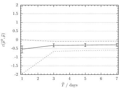
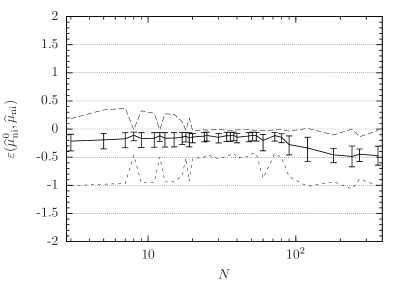
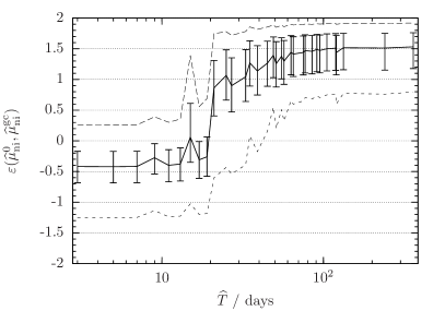
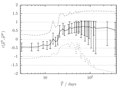
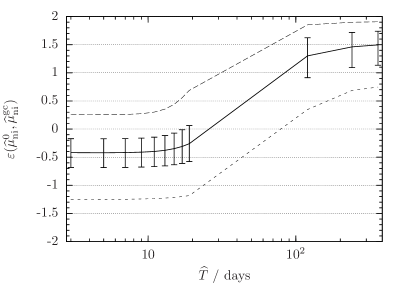
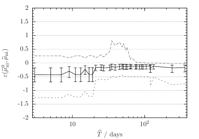
Figure 3: Relative errors ε(μ^ni0,μ^ni)𝜀subscriptsuperscript^𝜇0nisubscript^𝜇ni\varepsilon(\widehat{\mu}^{0}_{\textrm{ni}},\widehat{\mu}_{\textrm{ni}}) (left column) and ε(μ^0,μ^)𝜀superscript^𝜇0^𝜇\varepsilon(\widehat{\mu}^{0},\widehat{\mu}) (right column), at constant LABEL:sub@fig:mu_re_twoF_rssky_semiT_noiLABEL:sub@fig:mu_re_twoF_rssky_semiT_tot total time-span T^^𝑇\widehat{T}, LABEL:sub@fig:mu_re_twoF_rssky_cohT_noiLABEL:sub@fig:mu_re_twoF_rssky_cohT_tot segment time-span T~~𝑇\widetilde{T}, and LABEL:sub@fig:mu_re_twoF_rssky_N_noiLABEL:sub@fig:mu_re_twoF_rssky_N_tot number of segments N𝑁N. All other simulation parameters are averaged over. Plotted are the median (solid line), the 25th–75th percentile range (error bars), and the 2.5th (lower, short-dashed line) and 97.5th (upper, long-dashed line) percentiles.
Refer to caption
(a)
Refer to caption
(b)
Refer to caption
(c)
Refer to caption
(d)
Refer to caption
(e)
Refer to caption
(f)
Figure 4: Relative errors ε(μ^ni0,μ^ni)𝜀subscriptsuperscript^𝜇0nisubscript^𝜇ni\varepsilon(\widehat{\mu}^{0}_{\textrm{ni}},\widehat{\mu}_{\textrm{ni}}) (left column), and ε(μ^0,μ^)𝜀superscript^𝜇0^𝜇\varepsilon(\widehat{\mu}^{0},\widehat{\mu}) (right column), at constant LABEL:sub@fig:mu_re_twoF_rssky_semimumax_noiLABEL:sub@fig:mu_re_twoF_rssky_semimumax_tot maximum semicoherent template bank mismatch μ^maxsubscript^𝜇max\widehat{\mu}_{\textrm{max}}, LABEL:sub@fig:mu_re_twoF_rssky_cohmumax_noiLABEL:sub@fig:mu_re_twoF_rssky_cohmumax_tot maximum coherent template bank mismatch μ~maxsubscript~𝜇max\widetilde{\mu}_{\textrm{max}}, and LABEL:sub@fig:mu_re_twoF_rssky_eta_noiLABEL:sub@fig:mu_re_twoF_rssky_eta_tot segment duty cycle η=NT~/T^𝜂𝑁~𝑇^𝑇\eta=N\widetilde{T}/\widehat{T}. All other simulation parameters are averaged over. Plotted are the median (solid line), the 25th–75th percentile range (error bars), and the 2.5th (lower, short-dashed line) and 97.5th (upper, long-dashed line) percentiles.
Refer to caption
(a)
Refer to caption
(b)
Refer to caption
(c)
Refer to caption
(d)
Refer to caption
(e)
Refer to caption
(f)
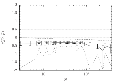
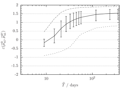
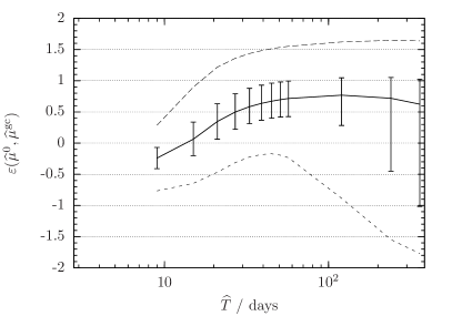
Figure 5: Relative errors ε(μ^ni0,μ^ni)𝜀subscriptsuperscript^𝜇0nisubscript^𝜇ni\varepsilon(\widehat{\mu}^{0}_{\textrm{ni}},\widehat{\mu}_{\textrm{ni}}) (left column) and ε(μ^0,μ^)𝜀superscript^𝜇0^𝜇\varepsilon(\widehat{\mu}^{0},\widehat{\mu}) (right column), at constant LABEL:sub@fig:mu_re_twoF_rssky_semiT_cohTgt1_noiLABEL:sub@fig:mu_re_twoF_rssky_semiT_cohTgt1_tot total time-span T^^𝑇\widehat{T}, LABEL:sub@fig:mu_re_twoF_rssky_cohT_cohTgt1_noiLABEL:sub@fig:mu_re_twoF_rssky_cohT_cohTgt1_tot segment time-span T~~𝑇\widetilde{T}, and LABEL:sub@fig:mu_re_twoF_rssky_N_cohTgt1_noiLABEL:sub@fig:mu_re_twoF_rssky_N_cohTgt1_tot number of segments N𝑁N. All other simulation parameters are averaged over, subject to the restriction T~>1~𝑇1\widetilde{T}>1 day. Plotted are the median (solid line), the 25th–75th percentile range (error bars), and the 2.5th (lower, short-dashed line) and 97.5th (upper, long-dashed line) percentiles.
Refer to caption
(a)
Refer to caption
(b)
Refer to caption
(c)
Refer to caption
(d)
Refer to caption
(e)
Refer to caption
(f)
Figure 6: Relative errors ε(μ^ni0,μ^ni)𝜀subscriptsuperscript^𝜇0nisubscript^𝜇ni\varepsilon(\widehat{\mu}^{0}_{\textrm{ni}},\widehat{\mu}_{\textrm{ni}}) (left column), and ε(μ^0,μ^)𝜀superscript^𝜇0^𝜇\varepsilon(\widehat{\mu}^{0},\widehat{\mu}) (right column), at constant LABEL:sub@fig:mu_re_twoF_rssky_semimumax_cohTgt1_noiLABEL:sub@fig:mu_re_twoF_rssky_semimumax_cohTgt1_tot maximum semicoherent template bank mismatch μ^maxsubscript^𝜇max\widehat{\mu}_{\textrm{max}}, LABEL:sub@fig:mu_re_twoF_rssky_cohmumax_cohTgt1_noiLABEL:sub@fig:mu_re_twoF_rssky_cohmumax_cohTgt1_tot maximum coherent template bank mismatch μ~maxsubscript~𝜇max\widetilde{\mu}_{\textrm{max}}, and LABEL:sub@fig:mu_re_twoF_rssky_eta_cohTgt1_noiLABEL:sub@fig:mu_re_twoF_rssky_eta_cohTgt1_tot segment duty cycle η=NT~/T^𝜂𝑁~𝑇^𝑇\eta=N\widetilde{T}/\widehat{T}. All other simulation parameters are averaged over, subject to the restriction T~>1~𝑇1\widetilde{T}>1 day. Plotted are the median (solid line), the 25th–75th percentile range (error bars), and the 2.5th (lower, short-dashed line) and 97.5th (upper, long-dashed line) percentiles.

Following Paper I, two mismatches μ0superscript𝜇0\mu^{0} and μ𝜇\mu are compared by plotting their relative error

ε(μ0,μ)μ0μ0.5(μ0+μ),μ0,μ0.formulae-sequence𝜀superscript𝜇0𝜇superscript𝜇0𝜇0.5superscript𝜇0𝜇superscript𝜇0𝜇0\varepsilon(\mu^{0},\mu)\equiv\frac{\mu^{0}-\mu}{0.5(\mu^{0}+\mu)}\,,\quad\mu^{0},\mu\geq 0\,. (36)

If ε(μ0,μ)<0𝜀superscript𝜇0𝜇0\varepsilon(\mu^{0},\mu)<0, then the metric mismatch μ𝜇\mu over-estimates the true \mathcal{F}-statistic mismatch μ0superscript𝜇0\mu^{0}. This implies that the metric is a conservative estimator of the \mathcal{F}-statistic mismatch, and therefore will restrict μ0μmaxsuperscript𝜇0subscript𝜇max\mu^{0}\leq\mu_{\textrm{max}} to less than the maximum metric mismatch μmaxsubscript𝜇max\mu_{\textrm{max}} prescribed by the template bank. If ε(μ0,μ)>0𝜀superscript𝜇0𝜇0\varepsilon(\mu^{0},\mu)>0, then μ𝜇\mu under-estimates μ0superscript𝜇0\mu^{0}; this implies that the metric is an optimistic estimator of the \mathcal{F}-statistic mismatch, and therefore may allow μ0>μmaxsuperscript𝜇0subscript𝜇max\mu^{0}>\mu_{\textrm{max}}. The behavior of the relative error can depend on how the parameter-space offsets, e.g. Δs𝝀^superscriptΔs^𝝀\Delta^{\mathrm{s}}\widehat{\boldsymbol{\lambda}}, are generated; see Figure 1 of Paper I. If, for example, the ellipsoid Δs𝝀^𝐠^0(𝓐,𝝀s)Δs𝝀^μ^maxsuperscriptΔs^𝝀superscript^𝐠0𝓐superscript𝝀ssuperscriptΔs^𝝀subscript^𝜇max\Delta^{\mathrm{s}}\widehat{\boldsymbol{\lambda}}\cdot\widehat{\boldsymbol{\mathrm{g}}}^{0}(\boldsymbol{\mathcal{A}},\boldsymbol{\lambda}^{\mathrm{s}})\cdot\Delta^{\mathrm{s}}\widehat{\boldsymbol{\lambda}}\leq\widehat{\mu}_{\textrm{max}} (where 𝐠^0(𝓐,𝝀s)==1N𝐠~0(𝓐,𝝀s)superscript^𝐠0𝓐superscript𝝀ssuperscriptsubscript1𝑁superscriptsubscript~𝐠0𝓐superscript𝝀s\widehat{\boldsymbol{\mathrm{g}}}^{0}(\boldsymbol{\mathcal{A}},\boldsymbol{\lambda}^{\mathrm{s}})=\sum_{\ell=1}^{N}\widetilde{\boldsymbol{\mathrm{g}}}_{\ell}^{0}(\boldsymbol{\mathcal{A}},\boldsymbol{\lambda}^{\mathrm{s}})) differs in orientation from the ellipsoid Δs𝝀^𝐠^Δs𝝀^μ^maxsuperscriptΔs^𝝀^𝐠superscriptΔs^𝝀subscript^𝜇max\Delta^{\mathrm{s}}\widehat{\boldsymbol{\lambda}}\cdot\widehat{\boldsymbol{\mathrm{g}}}\cdot\Delta^{\mathrm{s}}\widehat{\boldsymbol{\lambda}}\leq\widehat{\mu}_{\textrm{max}}, from which Δs𝝀^superscriptΔs^𝝀\Delta^{\mathrm{s}}\widehat{\boldsymbol{\lambda}} are sampled, this will tend to ε(μ^ni0,μ^ni)<0𝜀subscriptsuperscript^𝜇0nisubscript^𝜇ni0\varepsilon(\widehat{\mu}^{0}_{\textrm{ni}},\widehat{\mu}_{\textrm{ni}})<0.

Figures 3 and 4 plot the relative error between μ^ni0subscriptsuperscript^𝜇0ni\widehat{\mu}^{0}_{\textrm{ni}} and μ^nisubscript^𝜇ni\widehat{\mu}_{\textrm{ni}}, ε(μ^ni0,μ^ni)𝜀subscriptsuperscript^𝜇0nisubscript^𝜇ni\varepsilon(\widehat{\mu}^{0}_{\textrm{ni}},\widehat{\mu}_{\textrm{ni}}), and between μ^0superscript^𝜇0\widehat{\mu}^{0} and μ^^𝜇\widehat{\mu}, ε(μ^0,μ^)𝜀superscript^𝜇0^𝜇\varepsilon(\widehat{\mu}^{0},\widehat{\mu}). Overall, the metric 𝐠^^𝐠\widehat{\boldsymbol{\mathrm{g}}} is a good predictor of the \mathcal{F}-statistic mismatch: with no interpolation, the average median |ε(μ^ni0,μ^ni)|0.20similar-to𝜀subscriptsuperscript^𝜇0nisubscript^𝜇ni0.20|\varepsilon(\widehat{\mu}^{0}_{\textrm{ni}},\widehat{\mu}_{\textrm{ni}})|\sim 0.20, and the average 25th–75th percentile range 0.04similar-toabsent0.04\sim 0.04; with interpolation, the average median |ε(μ^0,μ^)|0.35similar-to𝜀superscript^𝜇0^𝜇0.35|\varepsilon(\widehat{\mu}^{0},\widehat{\mu})|\sim 0.35, and the average 25th–75th percentile range 0.03similar-toabsent0.03\sim 0.03. The magnitudes of the relative errors with interpolation are generally larger than those without interpolation, due to the mismatch between 𝝀ssuperscript𝝀s\boldsymbol{\lambda}^{\mathrm{s}} and 𝝀~(𝝀^)subscript~𝝀^𝝀\widetilde{\boldsymbol{\lambda}}_{\ell}(\widehat{\boldsymbol{\lambda}}) being generally larger than that between 𝝀^^𝝀\widehat{\boldsymbol{\lambda}} and 𝝀~(𝝀^)subscript~𝝀^𝝀\widetilde{\boldsymbol{\lambda}}_{\ell}(\widehat{\boldsymbol{\lambda}}); it was observed in Paper I that the predictions of the metric worsen at higher mismatches. The relative error magnitudes are mostly indifferent to changes in the various simulation parameters plotted in Fig. 4.

In general, the metric 𝐠^^𝐠\widehat{\boldsymbol{\mathrm{g}}} over-estimates the \mathcal{F}-statistic mismatch. The dominant contribution to this effect is the Taylor expansion in Eq.(5) of the \mathcal{F}-statistic mismatch, used in deriving the metric 𝐠~0(𝓐,𝝀s)superscriptsubscript~𝐠0𝓐superscript𝝀s\widetilde{\boldsymbol{\mathrm{g}}}_{\ell}^{0}(\boldsymbol{\mathcal{A}},\boldsymbol{\lambda}^{\mathrm{s}}) of which 𝐠~subscript~𝐠\widetilde{\boldsymbol{\mathrm{g}}}_{\ell} is an approximation; since 𝐠^^𝐠\widehat{\boldsymbol{\mathrm{g}}} is a function of 𝐠~subscript~𝐠\widetilde{\boldsymbol{\mathrm{g}}}_{\ell} by Eq. (33), it assumes the same approximation. Since this expansion is of second order, the metric mismatch μ^^𝜇\widehat{\mu} increases quadratically (see e.g. Figs. 11–12 in Prix (2007a)), while the \mathcal{F}-statistic mismatch μ^0superscript^𝜇0\widehat{\mu}^{0} is known to increase at a slower rate (see e.g. Fig. 10 in Prix (2007a), and Fig. 7 in Paper I). In addition, μ^^𝜇\widehat{\mu} is unbounded, while μ^0superscript^𝜇0\widehat{\mu}^{0} is by construction restricted to μ^01superscript^𝜇01\widehat{\mu}^{0}\leq 1. This general behavior is common to all parameter-space metrics based on a second-order Taylor expansion; see e.g. Prix (2007a); Keppel (2012), and Paper I. In addition, as noted above, the behavior of the relative error itself is biased to reporting over-estimation when the orientation of the metric ellipsoid of 𝐠^^𝐠\widehat{\boldsymbol{\mathrm{g}}} differs from that of 𝐠^0(𝓐,𝝀s)superscript^𝐠0𝓐superscript𝝀s\widehat{\boldsymbol{\mathrm{g}}}^{0}(\boldsymbol{\mathcal{A}},\boldsymbol{\lambda}^{\mathrm{s}}).

Figures 5 and 6 plot the same quantities as Figs. 3 and 4, but subject to the restriction T~>1~𝑇1\widetilde{T}>1 day. This restriction improves the predictions of 𝐠^^𝐠\widehat{\boldsymbol{\mathrm{g}}}: with no interpolation, the average median |ε(μ^ni0,μ^ni)|0.13similar-to𝜀subscriptsuperscript^𝜇0nisubscript^𝜇ni0.13|\varepsilon(\widehat{\mu}^{0}_{\textrm{ni}},\widehat{\mu}_{\textrm{ni}})|\sim 0.13, and the average 25th–75th percentile range 0.03similar-toabsent0.03\sim 0.03; with interpolation, the average median |ε(μ^0,μ^)|0.30similar-to𝜀superscript^𝜇0^𝜇0.30|\varepsilon(\widehat{\mu}^{0},\widehat{\mu})|\sim 0.30, and the average 25th–75th percentile range 0.007similar-toabsent0.007\sim 0.007. Many of the outlying relative errors seen in Figs. 3 and 4 are also removed by this restriction: compare the 2.5th percentile lines in Figs. 5a and 5b vs. Figs. 3a and 3b; in Figs. 5e and 5f vs. Figs. 3e and 3f; and Figs. 6e and 6f vs. Figs. 4e and 4f.

As noted in Paper I, the predictions of 𝐠~subscript~𝐠\widetilde{\boldsymbol{\mathrm{g}}}_{\ell} are worse at T~=1~𝑇1\widetilde{T}=1 day for two reasons. First, the phase metric 𝐠~ϕ(𝝀s)superscriptsubscript~𝐠italic-ϕsuperscript𝝀s\widetilde{\boldsymbol{\mathrm{g}}}_{\ell}^{\phi}(\boldsymbol{\lambda}^{\mathrm{s}}) approximates 𝐠~0(𝓐,𝝀s)superscriptsubscript~𝐠0𝓐superscript𝝀s\widetilde{\boldsymbol{\mathrm{g}}}_{\ell}^{0}(\boldsymbol{\mathcal{A}},\boldsymbol{\lambda}^{\mathrm{s}}) in Eq. (8) in part by neglecting the amplitude modulation of the signal of a gravitational-wave pulsar; since these modulations arise primarily from the rotation of the Earth, this approximation is worst at T~1similar-to~𝑇1\widetilde{T}\sim 1 day. Second, the numerical ill-conditionedness of the phase metric (see Prix (2007a) and Paper I) increases the difficulty of computing 𝐠~usuperscriptsubscript~𝐠u\widetilde{\boldsymbol{\mathrm{g}}}_{\ell}^{\textrm{u}}, from which both 𝐠~subscript~𝐠\widetilde{\boldsymbol{\mathrm{g}}}_{\ell} and 𝐠^^𝐠\widehat{\boldsymbol{\mathrm{g}}} are derived, at smaller T~~𝑇\widetilde{T}.

One feature of interest is the 2.5th percentile lines in Figs. 5b and 5f. At this line, ε(μ^0,μ^)2similar-to𝜀superscript^𝜇0^𝜇2\varepsilon(\widehat{\mu}^{0},\widehat{\mu})\sim-2 at T^10similar-to^𝑇10\widehat{T}\sim 10 days and N3similar-to𝑁3N\sim 3, but reduces to ε(μ^0,μ^)1similar-to𝜀superscript^𝜇0^𝜇1\varepsilon(\widehat{\mu}^{0},\widehat{\mu})\sim-1 for T^40greater-than-or-equivalent-to^𝑇40\widehat{T}\gtrsim 40 days and N6greater-than-or-equivalent-to𝑁6N\gtrsim 6. The general decrease in ε(μ^0,μ^)𝜀superscript^𝜇0^𝜇\varepsilon(\widehat{\mu}^{0},\widehat{\mu}) is simply due to the larger number of segments N𝑁N (since T^^𝑇\widehat{T} is approximately Nproportional-toabsent𝑁\propto N), which mitigates the effect of a large over-estimation of the \mathcal{F}-statistic mismatch in any one segment. (The momentary increase in ε(μ^0,μ^)𝜀superscript^𝜇0^𝜇\varepsilon(\widehat{\mu}^{0},\widehat{\mu}) along the 2.5th percentile line in Fig. 5b for 30T^/days60less-than-or-similar-to30^𝑇daysless-than-or-similar-to6030\lesssim\widehat{T}/\textrm{days}\lesssim 60 is explained in the next section.)

The jumps in the relative errors seen in Figs. 3e, 3f, 5e, and 5f – most noticeably in the 2.5th and 97.5th percentile lines – are artifacts of plotting the 72 search setups with respect to N𝑁N. For example, note that in Fig. 3f the magnitude and spread of the relative error is noticeably less at N=8𝑁8N=8 than at either N=7𝑁7N=7 or N=9𝑁9N=9. From Table 2, the only setup with N=8𝑁8N=8 is that with T^=120^𝑇120\widehat{T}=120 days, while the setups at N=7𝑁7N=7 and N=9𝑁9N=9 have T^49^𝑇49\widehat{T}\leq 49 days and T^63^𝑇63\widehat{T}\leq 63 days respectively. Given that the metric predictions improve with T^^𝑇\widehat{T}, it is expected that the relative error at N=8𝑁8N=8 is reduced relative to N=7𝑁7N=7 or N=9𝑁9N=9.

III.2.3 Simulation results: metric under-estimation
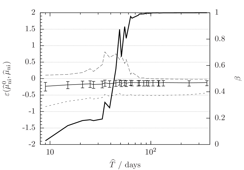
Refer to caption
Figure 7: Relative errors ε(μ^ni0,μ^ni)𝜀subscriptsuperscript^𝜇0nisubscript^𝜇ni\varepsilon(\widehat{\mu}^{0}_{\textrm{ni}},\widehat{\mu}_{\textrm{ni}}) (left y-axis) at constant total time-span T^^𝑇\widehat{T}, as in Fig. 5a. Overplotted in black is the orientation angle β𝛽\beta (right y-axis) of the plane of the reduced supersky coordinates (n~a,n~b)subscript~𝑛𝑎subscript~𝑛𝑏(\widetilde{n}_{a},\widetilde{n}_{b}).
Refer to caption
(a)
Refer to caption
(b)
Figure 8: Intensity maps of the probabilities LABEL:sub@fig:mu_underest_skymap_sseg_noi p(ε(μ^ni0,μ^ni)>0)𝑝𝜀subscriptsuperscript^𝜇0nisubscript^𝜇ni0p\big{(}\varepsilon(\widehat{\mu}^{0}_{\textrm{ni}},\widehat{\mu}_{\textrm{ni}})>0\big{)} and LABEL:sub@fig:mu_underest_skymap_sseg_tot p(ε(μ^0,μ^)>0)𝑝𝜀superscript^𝜇0^𝜇0p\big{(}\varepsilon(\widehat{\mu}^{0},\widehat{\mu})>0\big{)}, as functions of right ascension α𝛼\alpha and declination δ𝛿\delta, for the 36 setups listed in the top half of Table 2. The remaining simulation parameters, f𝑓f and (μ~max,μ^max)subscript~𝜇maxsubscript^𝜇max(\widetilde{\mu}_{\textrm{max}},\widehat{\mu}_{\textrm{max}}), are averaged over. Overplotted are the ecliptic equator (black line), and the positions of the LIGO Livingston detector at the start times of the first (black dot) and last (black cross) segments. Each map is titled by the triplet (N𝑁N, T~~𝑇\widetilde{T} / days, η𝜂\eta). The maps are normalized such that the total probability in each map is either LABEL:sub@fig:mu_underest_skymap_sseg_noi 10Sni0superscript10subscriptsuperscript𝑆0ni10^{-S^{0}_{\textrm{ni}}} or LABEL:sub@fig:mu_underest_skymap_sseg_tot 10S0superscript10superscript𝑆010^{-S^{0}}, where Sni0subscriptsuperscript𝑆0niS^{0}_{\textrm{ni}} and S0superscript𝑆0S^{0} are given for each setup in Table 2.
Refer to caption
(a)
Refer to caption
(b)
Figure 9: Intensity maps of the probabilities LABEL:sub@fig:mu_underest_skymap_sseg_noi p(ε(μ^ni0,μ^ni)>0)𝑝𝜀subscriptsuperscript^𝜇0nisubscript^𝜇ni0p\big{(}\varepsilon(\widehat{\mu}^{0}_{\textrm{ni}},\widehat{\mu}_{\textrm{ni}})>0\big{)} and LABEL:sub@fig:mu_underest_skymap_sseg_tot p(ε(μ^0,μ^)>0)𝑝𝜀superscript^𝜇0^𝜇0p\big{(}\varepsilon(\widehat{\mu}^{0},\widehat{\mu})>0\big{)}, as functions of right ascension α𝛼\alpha and declination δ𝛿\delta, for the 36 setups listed in the bottom half of Table 2. The remaining simulation parameters, f𝑓f and (μ~max,μ^max)subscript~𝜇maxsubscript^𝜇max(\widetilde{\mu}_{\textrm{max}},\widehat{\mu}_{\textrm{max}}), are averaged over. Overplotted is the ecliptic equator (black line). Each map is titled by the triplet (T^^𝑇\widehat{T} / days, T~~𝑇\widetilde{T} / days, η𝜂\eta). The maps are normalized such that the total probability in each map is either LABEL:sub@fig:mu_underest_skymap_sseg_noi 10Sni0superscript10subscriptsuperscript𝑆0ni10^{-S^{0}_{\textrm{ni}}} or LABEL:sub@fig:mu_underest_skymap_sseg_tot 10S0superscript10superscript𝑆010^{-S^{0}}, where Sni0subscriptsuperscript𝑆0niS^{0}_{\textrm{ni}} and S0superscript𝑆0S^{0} are given for each setup in Table 2.

It is also possible for the metric 𝐠^^𝐠\widehat{\boldsymbol{\mathrm{g}}} to under-estimate the \mathcal{F}-statistic mismatch. It is important to note that, when performing a real search using an implementation of a lattice template bank, as e.g. described in Paper II, metric under-estimation may not necessarily lead to loss of coverage (i.e. areas of parameter space where μ^>μ^max^𝜇subscript^𝜇max\widehat{\mu}>\widehat{\mu}_{\textrm{max}}). For example, metric under-estimation at parameter-space boundaries may be compensated for by additional boundary templates. Tests of lattice template banks constructed using 𝐠~subscript~𝐠\widetilde{\boldsymbol{\mathrm{g}}}_{\ell} in Paper II have demonstrated that near-complete coverage is attainable using the reduced supersky metric.

Table 2 lists, for each of the 72 search setups, the probability that the semicoherent mismatches μ^0superscript^𝜇0\widehat{\mu}^{0} and μ^ni0subscriptsuperscript^𝜇0ni\widehat{\mu}^{0}_{\textrm{ni}} (i.e. with and without interpolation) will under-estimate the respective \mathcal{F}-statistic mismatches. The probabilities are given in logarithmic form by Sxlog10p(ε(μ^0,μ^)>x)superscript𝑆𝑥subscript10𝑝𝜀superscript^𝜇0^𝜇𝑥S^{x}\equiv-\log_{10}p\big{(}\varepsilon(\widehat{\mu}^{0},\widehat{\mu})>x\big{)} and Snixlog10p(ε(μ^ni0,μ^ni)>x)subscriptsuperscript𝑆𝑥nisubscript10𝑝𝜀subscriptsuperscript^𝜇0nisubscript^𝜇ni𝑥S^{x}_{\textrm{ni}}\equiv-\log_{10}p\big{(}\varepsilon(\widehat{\mu}^{0}_{\textrm{ni}},\widehat{\mu}_{\textrm{ni}})>x\big{)}, where x{0,0.5}𝑥00.5x\in\{0,0.5\}. We observe that the probability of under-estimation for any search setup is 10less-than-or-similar-toabsent10\lesssim 10% (i.e. Sx1greater-than-or-equivalent-tosuperscript𝑆𝑥1S^{x}\gtrsim 1), and decreases with increasing number of segments N𝑁N and coherent time-span T~~𝑇\widetilde{T}, and with the addition of interpolation. This is expected: increasing N𝑁N reduces the potential effect of 𝐠^^𝐠\widehat{\boldsymbol{\mathrm{g}}} under-estimating the \mathcal{F}-statistic mismatch in a few segments, as does the addition of interpolation which averages the coherent and semicoherent mismatches; and Figs. 3a and 3b demonstrate that 𝐠^^𝐠\widehat{\boldsymbol{\mathrm{g}}} better approximates the \mathcal{F}-statistic at larger T~~𝑇\widetilde{T}.

In Figures 3a and 5a, we can see that, at the 97.5th percentile line, μ^nisubscript^𝜇ni\widehat{\mu}_{\textrm{ni}} noticeably under-estimates μ^ni0subscriptsuperscript^𝜇0ni\widehat{\mu}^{0}_{\textrm{ni}} for 30T^/days60less-than-or-similar-to30^𝑇daysless-than-or-similar-to6030\lesssim\widehat{T}/\textrm{days}\lesssim 60. This is due to a known feature of the reduced supersky metric; see Section V D of Paper I. As the time T^^𝑇\widehat{T} spanned by the metric 𝐠^^𝐠\widehat{\boldsymbol{\mathrm{g}}} increases, the orientation of the plane of the reduced supersky coordinates (n^a,n^b)subscript^𝑛𝑎subscript^𝑛𝑏(\widehat{n}_{a},\widehat{n}_{b}) transitions from being perpendicular to the equatorial z𝑧z-axis to being perpendicular to the ecliptic Z𝑍Z axis; in other words, the (n^a,n^b)subscript^𝑛𝑎subscript^𝑛𝑏(\widehat{n}_{a},\widehat{n}_{b}) transition from “equatorial-like” coordinates to “ecliptic-like” coordinates. During this transition, the reduced supersky metric is more likely to under-estimate the \mathcal{F}-statistic mismatch; compare Fig. 3a and 5a to Fig. 14 of Paper I.

To illustrate the transition, Figure 7 overplots Fig. 5a with the orientation angle β𝛽\beta (given by Eq. (51) of Paper I) of the plane of the reduced supersky coordinates (n^a,n^b)subscript^𝑛𝑎subscript^𝑛𝑏(\widehat{n}_{a},\widehat{n}_{b}), normalized such that β=0𝛽0\beta=0 signifies an “equatorial-like” orientation and β=1𝛽1\beta=1 an “ecliptic-like” orientation. The transition from “equatorial-like” to “ecliptic-like” coordinates occurs between T^30similar-to^𝑇30\widehat{T}\sim 30 days and 60 days, the same domain where μ^nisubscript^𝜇ni\widehat{\mu}_{\textrm{ni}} noticeably under-estimates μ^ni0subscriptsuperscript^𝜇0ni\widehat{\mu}^{0}_{\textrm{ni}}. The momentary increase in ε(μ^0,μ^)𝜀superscript^𝜇0^𝜇\varepsilon(\widehat{\mu}^{0},\widehat{\mu}) along the 2.5th percentile line in Fig. 5b also occurs when 30T^/days60less-than-or-similar-to30^𝑇daysless-than-or-similar-to6030\lesssim\widehat{T}/\textrm{days}\lesssim 60, and therefore is also likely due to the transition.

To determine whether metric under-estimation is correlated with particular regions of parameter space, we identify pulsar sky positions, in terms of right ascension α𝛼\alpha and declination δ𝛿\delta, where the metric 𝐠^^𝐠\widehat{\boldsymbol{\mathrm{g}}} under-estimates the \mathcal{F}-statistic mismatch. Figures 8 and 9 map the probability of metric underestimation as a function of (α,δ)𝛼𝛿(\alpha,\delta), for each setup given in Table 2. The maps are normalized such that the total probability in each map is either 10Sni0superscript10subscriptsuperscript𝑆0ni10^{-S^{0}_{\textrm{ni}}} without interpolation (Figs. 8a and 9a), or 10S0superscript10superscript𝑆010^{-S^{0}} with interpolation (Figs. 8b and 9b), where Sni0subscriptsuperscript𝑆0niS^{0}_{\textrm{ni}} and S0superscript𝑆0S^{0} are given for each setup in Table 2. Two effects, which cause metric under-estimation to be concentrated in particular regions of the sky, are identified and explained in the following paragraphs.

First, for short segment time-spans T~3less-than-or-similar-to~𝑇3\widetilde{T}\lesssim 3 days, regions of the sky which (anti-)correlate with the position of the detector used in the numerical simulations – the LIGO Livingston detector – are more likely to result in metric under-estimation; see Figure 8. This is likely due to the neglect of the amplitude modulation of the gravitational-wave pulsar signal in deriving the phase metric 𝐠~ϕ(𝝀s)superscriptsubscript~𝐠italic-ϕsuperscript𝝀s\widetilde{\boldsymbol{\mathrm{g}}}_{\ell}^{\phi}(\boldsymbol{\lambda}^{\mathrm{s}}), as noted above in Section III.2.2. Without interpolation (Fig. 8a), where only the semicoherent metric 𝐠^^𝐠\widehat{\boldsymbol{\mathrm{g}}} is involved, the effect appears at T~1similar-to~𝑇1\widetilde{T}\sim 1 day and generally fades for longer T~~𝑇\widetilde{T} and more N𝑁N; with interpolation (Fig. 8b), where both 𝐠^^𝐠\widehat{\boldsymbol{\mathrm{g}}} and the coherent metrics 𝐠~subscript~𝐠\widetilde{\boldsymbol{\mathrm{g}}}_{\ell} are involved, the effect is most noticeable at T~3similar-to~𝑇3\widetilde{T}\sim 3 days. It is probable that the effect of neglecting the amplitude modulation becomes irrelevant more quickly for the semicoherent metric as N𝑁N increases and more coherent metrics are averaged together.

Second, at longer T~~𝑇\widetilde{T}, the probability of metric under-estimation becomes concentrated at either the ecliptic equator (without interpolation), or at the equatorial equator δ=0𝛿0\delta=0 (without interpolation); see Figures 8 and 9. This is likely due to the transition of the reduced supersky coordinates from “equatorial-like” coordinates to “ecliptic-like” coordinates, which begins at T^30greater-than-or-equivalent-to^𝑇30\widehat{T}\gtrsim 30 days for the semicoherent metric (see Section III.2.2 and Fig. 7), and at T~10greater-than-or-equivalent-to~𝑇10\widetilde{T}\gtrsim 10 days for the coherent metric (see Section V D of Paper I). In Figs. 8a and 9a (i.e. without interpolation), only the semicoherent metric 𝐠^^𝐠\widehat{\boldsymbol{\mathrm{g}}} is in use, and the maps are generally consistent with a transition from “equatorial-like” to “ecliptic-like” coordinates on the timescale T^30greater-than-or-equivalent-to^𝑇30\widehat{T}\gtrsim 30 days. In Figs. 8b and 9b (i.e. with interpolation), 𝐠^^𝐠\widehat{\boldsymbol{\mathrm{g}}} contributes only once to the total metric mismatch, whereas the coherent metrics 𝐠~subscript~𝐠\widetilde{\boldsymbol{\mathrm{g}}}_{\ell} contribute N1much-greater-than𝑁1N\gg 1 times; see the vector summation in Fig. 1. The maps therefore tend to reflect the behavior of the coherent metric, which for T~7~𝑇7\widetilde{T}\leq 7 days remains “equatorial-like”.

III.2.4 Simulation results: mismatch histograms

Refer to caption
(a)
Refer to caption
(b)
Refer to caption
(c)
Refer to caption
(d)
Refer to caption
(e)
Figure 10: Histograms in mismatches in: the coherent mismatches in each segment μ~0superscriptsubscript~𝜇0\widetilde{\mu}_{\ell}^{0}, μ~subscript~𝜇\widetilde{\mu}_{\ell} (left column); the semicoherent mismatches with no interpolation μ^ni0subscriptsuperscript^𝜇0ni\widehat{\mu}^{0}_{\textrm{ni}}, μ^nisubscript^𝜇ni\widehat{\mu}_{\textrm{ni}} (middle column); and the semicoherent mismatches with interpolation μ^0superscript^𝜇0\widehat{\mu}^{0}, μ^^𝜇\widehat{\mu} (right column). Histograms are at fixed maximum template-bank mismatches (μ~max,μ^max)subscript~𝜇maxsubscript^𝜇max(\widetilde{\mu}_{\textrm{max}},\widehat{\mu}_{\textrm{max}}) equal to LABEL:sub@fig:mu_hgrm_twoF_rssky_coh0p1_semi0p1 (0.1,0.1)0.10.1(0.1,0.1), LABEL:sub@fig:mu_hgrm_twoF_rssky_coh0p3_semi0p3 (0.3,0.3)0.30.3(0.3,0.3), LABEL:sub@fig:mu_hgrm_twoF_rssky_coh0p5_semi0p5 (0.5,0.5)0.50.5(0.5,0.5), LABEL:sub@fig:mu_hgrm_twoF_rssky_coh0p1_semi0p5 (0.1,0.5)0.10.5(0.1,0.5), LABEL:sub@fig:mu_hgrm_twoF_rssky_coh0p5_semi0p1 (0.5,0.1)0.50.1(0.5,0.1). All other simulation parameters are averaged over.

Figure 10 plots histograms of the coherent mismatches in each segment, μ~0superscriptsubscript~𝜇0\widetilde{\mu}_{\ell}^{0}, μ~subscript~𝜇\widetilde{\mu}_{\ell}, and the semicoherent mismatches with and without interpolation, μ^0superscript^𝜇0\widehat{\mu}^{0}, μ^^𝜇\widehat{\mu} and μ^ni0subscriptsuperscript^𝜇0ni\widehat{\mu}^{0}_{\textrm{ni}}, μ^nisubscript^𝜇ni\widehat{\mu}_{\textrm{ni}} respectively. The coherent mismatches reproduce the results obtained in Fig. 4 of Paper II. The histograms again demonstrate the conservative over-estimation of the metric approximation, in that the metric mismatch histograms (dashed lines in Fig. 10) are peaked at higher mismatches than the \mathcal{F}-statistic mismatch histograms (solid lines).

The shape of the histograms in μ~subscript~𝜇\widetilde{\mu}_{\ell} and μ^nisubscript^𝜇ni\widehat{\mu}_{\textrm{ni}} in Figure 10 conform to that expected for four-dimensional template banks constructed from an A4superscriptsubscript𝐴4A_{4}^{*} lattice; see Fig. 1 of Paper II. The shape of the histograms in μ^^𝜇\widehat{\mu}, to which both the coherent and semicoherent template bank mismatches contribute, is closer to a Gaussian in shape; this is likely due to the central limit theorem applying when the N𝑁N coherent mismatches μ~0(𝝀^;𝝀~(𝝀^))superscriptsubscript~𝜇0^𝝀subscript~𝝀^𝝀\widetilde{\mu}_{\ell}^{0}\big{(}\widehat{\boldsymbol{\lambda}};\widetilde{\boldsymbol{\lambda}}_{\ell}(\widehat{\boldsymbol{\lambda}})\big{)} are averaged in Eq. (29), assuming N𝑁N is sufficiently large. Note that, however, the histogram in μ^^𝜇\widehat{\mu} for (μ~max,μ^max)=(0.1,0.5)subscript~𝜇maxsubscript^𝜇max0.10.5(\widetilde{\mu}_{\textrm{max}},\widehat{\mu}_{\textrm{max}})=(0.1,0.5) (Fig. 10d) instead more closely resembles that of μ^nisubscript^𝜇ni\widehat{\mu}_{\textrm{ni}}, as might be expected since μ~maxμ^maxmuch-less-thansubscript~𝜇maxsubscript^𝜇max\widetilde{\mu}_{\textrm{max}}\ll\widehat{\mu}_{\textrm{max}}, i.e. the coherent template bank mismatches μ~subscript~𝜇\widetilde{\mu}_{\ell} contribute little to the total mismatch μ^^𝜇\widehat{\mu}.

IV Comparisons to previous work

Refer to caption
(a)
Refer to caption
(b)
Refer to caption
(c)
Refer to caption
(d)
Refer to caption
(e)
Refer to caption
(f)
Figure 11: Relative errors ε(μ^ni0,μ^nigc)𝜀subscriptsuperscript^𝜇0nisubscriptsuperscript^𝜇gcni\varepsilon(\widehat{\mu}^{0}_{\textrm{ni}},\widehat{\mu}^{\textrm{gc}}_{\textrm{ni}}) (left column) and ε(μ^0,μ^gc)𝜀superscript^𝜇0superscript^𝜇gc\varepsilon(\widehat{\mu}^{0},\widehat{\mu}^{\textrm{gc}}) (right column), at constant total time-span T^^𝑇\widehat{T}. All other simulation parameters are averaged over, subject to the following restrictions on the search setups listed in Table 2: LABEL:sub@fig:mu_re_twoF_gctco_semiT_noiLABEL:sub@fig:mu_re_twoF_gctco_semiT_tot no restrictions; LABEL:sub@fig:mu_re_twoF_gctco_semiT_cohTeq1_dutyeq1_noiLABEL:sub@fig:mu_re_twoF_gctco_semiT_cohTeq1_dutyeq1_tot T~=1~𝑇1\widetilde{T}=1 day, η=1𝜂1\eta=1; and LABEL:sub@fig:mu_re_twoF_gctco_semiT_cohTeq3_dutyeq1_noiLABEL:sub@fig:mu_re_twoF_gctco_semiT_cohTeq3_dutyeq1_tot T~=3~𝑇3\widetilde{T}=3 days, η=1𝜂1\eta=1. Plotted are the median (solid line), the 25th–75th percentile range (error bars), and the 2.5th (lower, short-dashed line) and 97.5th (upper, long-dashed line) percentiles.

Section IV.1 compares the semicoherent metric 𝐠^^𝐠\widehat{\boldsymbol{\mathrm{g}}}, presented in the previous section, to the global correlation metric of Pletsch (2010). Section IV.2 compares predictions for the number of semicoherent templates given by 𝐠^^𝐠\widehat{\boldsymbol{\mathrm{g}}} to predictions given by Brady and Creighton (2000); Pletsch (2010).
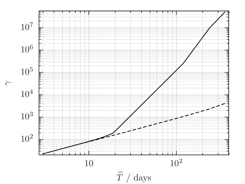
Refer to caption
Figure 12: Refinement of the supersky metric given by Eq. (37) (solid line), and of the global correlation metric given by Pletsch (2010) (dashed line), as a function of total time-span T^^𝑇\widehat{T}. The search setups listed in Table 2 are restricted to T~=1~𝑇1\widetilde{T}=1 day and η=1𝜂1\eta=1.
Refer to caption
Figure 13: Number of semicoherent templates predicted by the supersky metric (solid line), by the global correlation metric of Pletsch (2010) (dashed line), and by Brady and Creighton (2000) (dash-dotted line), as a function of total time-span T^^𝑇\widehat{T}. The search setups listed in Table 2 are restricted to T~=1~𝑇1\widetilde{T}=1 day and η=1𝜂1\eta=1.

IV.1 Comparison to the global correlation metric

The numerical simulations described in Section III.2 were repeated with two changes: the coherent global correlation metrics 𝐠~gcsuperscriptsubscript~𝐠gc\widetilde{\boldsymbol{\mathrm{g}}}_{\ell}^{\textrm{gc}} given by Eqs. (50) of Pletsch (2010) were substituted for the coherent supersky metrics 𝐠~subscript~𝐠\widetilde{\boldsymbol{\mathrm{g}}}_{\ell}, and the semicoherent global correlation metric 𝐠^gcsuperscript^𝐠gc\widehat{\boldsymbol{\mathrm{g}}}^{\textrm{gc}} given by Eqs. (59) of Pletsch (2010) was substituted for the semicoherent supersky metric 𝐠^^𝐠\widehat{\boldsymbol{\mathrm{g}}}. In other words, the simulations were repeated assuming that the global correlation metrics are used to construct the coherent and semicoherent template banks in steps (ii) and (iv) of the procedure described in Section III.2.

Figure 11 plots the relative error between μ^ni0subscriptsuperscript^𝜇0ni\widehat{\mu}^{0}_{\textrm{ni}} and μ^nigcsubscriptsuperscript^𝜇gcni\widehat{\mu}^{\textrm{gc}}_{\textrm{ni}}, ε(μ^ni0,μ^nigc)𝜀subscriptsuperscript^𝜇0nisubscriptsuperscript^𝜇gcni\varepsilon(\widehat{\mu}^{0}_{\textrm{ni}},\widehat{\mu}^{\textrm{gc}}_{\textrm{ni}}), and between μ^0superscript^𝜇0\widehat{\mu}^{0} and μ^gcsuperscript^𝜇gc\widehat{\mu}^{\textrm{gc}}, ε(μ^0,μ^gc)𝜀superscript^𝜇0superscript^𝜇gc\varepsilon(\widehat{\mu}^{0},\widehat{\mu}^{\textrm{gc}}). Figs. 11a and 11b are directly comparable to Figs. 3a and 3b for the supersky metrics respectively. The global correlation metric over-estimates the \mathcal{F}-statistic mismatch, with the median |ε(μ^ni0,μ^nigc)||ε(μ^0,μ^gc)|0.4similar-to𝜀subscriptsuperscript^𝜇0nisubscriptsuperscript^𝜇gcni𝜀superscript^𝜇0superscript^𝜇gcless-than-or-similar-to0.4|\varepsilon(\widehat{\mu}^{0}_{\textrm{ni}},\widehat{\mu}^{\textrm{gc}}_{\textrm{ni}})|\sim|\varepsilon(\widehat{\mu}^{0},\widehat{\mu}^{\textrm{gc}})|\lesssim 0.4, provided that T^20less-than-or-similar-to^𝑇20\widehat{T}\lesssim 20 days; for T^20greater-than-or-equivalent-to^𝑇20\widehat{T}\gtrsim 20 days, the global correlation metric severely under-estimates the \mathcal{F}-statistic mismatch, with the median ε(μ^ni0,μ^nigc)1greater-than-or-equivalent-to𝜀subscriptsuperscript^𝜇0nisubscriptsuperscript^𝜇gcni1\varepsilon(\widehat{\mu}^{0}_{\textrm{ni}},\widehat{\mu}^{\textrm{gc}}_{\textrm{ni}})\gtrsim 1 and ε(μ^0,μ^gc)0.5greater-than-or-equivalent-to𝜀superscript^𝜇0superscript^𝜇gc0.5\varepsilon(\widehat{\mu}^{0},\widehat{\mu}^{\textrm{gc}})\gtrsim 0.5. Figs. 11c11f restrict the search setups listed in Table 2 to T~{1,3}~𝑇13\widetilde{T}\in\{1,3\} days and η=1𝜂1\eta=1 (i.e. contiguous segments). The behavior of the median relative error is similar under these restrictions: in Fig. 11d, ε(μ^0,μ^gc)0greater-than-or-equivalent-to𝜀superscript^𝜇0superscript^𝜇gc0\varepsilon(\widehat{\mu}^{0},\widehat{\mu}^{\textrm{gc}})\gtrsim 0 for T^20greater-than-or-equivalent-to^𝑇20\widehat{T}\gtrsim 20 days and ε(μ^0,μ^gc)0.5greater-than-or-equivalent-to𝜀superscript^𝜇0superscript^𝜇gc0.5\varepsilon(\widehat{\mu}^{0},\widehat{\mu}^{\textrm{gc}})\gtrsim 0.5 for T^120greater-than-or-equivalent-to^𝑇120\widehat{T}\gtrsim 120 days; in Fig. 11f, ε(μ^0,μ^gc)0greater-than-or-equivalent-to𝜀superscript^𝜇0superscript^𝜇gc0\varepsilon(\widehat{\mu}^{0},\widehat{\mu}^{\textrm{gc}})\gtrsim 0 for T^14greater-than-or-equivalent-to^𝑇14\widehat{T}\gtrsim 14 days and ε(μ^0,μ^gc)0.5greater-than-or-equivalent-to𝜀superscript^𝜇0superscript^𝜇gc0.5\varepsilon(\widehat{\mu}^{0},\widehat{\mu}^{\textrm{gc}})\gtrsim 0.5 for T^30greater-than-or-equivalent-to^𝑇30\widehat{T}\gtrsim 30 days.

The relationship between the semicoherent and coherent metrics is often quantified using the refinement,

γdet𝐠^median{det𝐠~}.𝛾^𝐠subscriptmediansubscript~𝐠\gamma\equiv\frac{\sqrt{\det\widehat{\boldsymbol{\mathrm{g}}}}}{\operatorname{median}_{\ell}\{\sqrt{\det\widetilde{\boldsymbol{\mathrm{g}}}_{\ell}}\}}\,. (37)

This quantifies the ratio of the number of templates in the semicoherent template bank 𝒩^det𝐠^proportional-to^𝒩^𝐠\widehat{\mathcal{N}}\propto\sqrt{\det\widehat{\boldsymbol{\mathrm{g}}}} to the median 555 In contrast to e.g. Pletsch (2010), we use the median rather than the mean in the denominator of Eq. (37), for the following reason. Throughout this paper we calculate detector positions 𝒓(t)𝒓𝑡\boldsymbol{r}(t) [Eq. (9)] using standard Jet Propulsion Laboratory ephemerides for the motion of the Earth and Sun. For segments with T~1similar-to~𝑇1\widetilde{T}\sim 1 day and specific segment mid-times, the ephemeris-derived orbital motion of the Earth can potentially interact with step (ii) of the procedure described in Section II.2 to predict anomalously large numbers of coherent templates. Using the median instead of the mean, therefore, gives a more representative value for the refinement in these circumstances. number of templates in the coherent template banks 𝒩~det𝐠~proportional-tosubscript~𝒩subscript~𝐠\widetilde{\mathcal{N}}_{\ell}\propto\sqrt{\det\widetilde{\boldsymbol{\mathrm{g}}}_{\ell}}, assuming μ^max=μ~maxsubscript^𝜇maxsubscript~𝜇max\widehat{\mu}_{\textrm{max}}=\widetilde{\mu}_{\textrm{max}}. Figure 12 plots the refinement for both supersky and global correlation metrics, the former given by Eq. (37), the latter given by Eqs. (50), (59), and (73) of Pletsch (2010). The search setups listed in Table 2 are restricted to T~=1~𝑇1\widetilde{T}=1 day and η=1𝜂1\eta=1. For T^20greater-than-or-equivalent-to^𝑇20\widehat{T}\gtrsim 20 days, the rate of increase of the supersky metric refinement increases markedly, while that of the global correlation metric refinement remains constant. The lack of additional refinement by the global correlation metric for T^20greater-than-or-equivalent-to^𝑇20\widehat{T}\gtrsim 20 days is consistent with the deterioration in its ability to predict the \mathcal{F}-statistic mismatch above the same threshold, as observed in Fig. 11.

The semicoherent global correlation metric is derived under a number of assumptions, which were studied in unpublished work by Manca (2013). One assumption is that the sky position parameters do not contribute to the refinement, i.e. that the number of distinct sky positions that must be searched remains the same in both the semicoherent and coherent template banks. We conclude from Figs. 11 and 12, however, that this assumption remains valid only for T^20less-than-or-similar-to^𝑇20\widehat{T}\lesssim 20 days. That the sky position parameters do contribute to the refinement has also been found in work on the Hough method, a similar semicoherent search method for gravitational-wave pulsars Krishnan et al. (2004); Astone et al. (2014).

IV.2 Number of semicoherent templates

Figure 13 plots the number of semicoherent templates 𝒩^^𝒩\widehat{\mathcal{N}} required to search the whole sky, frequencies up to fmaxsubscript𝑓maxf_{\textrm{max}}, and spindowns |f˙|f/τmin˙𝑓𝑓subscript𝜏min|\dot{f}|\leq f/\tau_{\textrm{min}} (motivated by a minimum “spindown age” of the gravitational-wave pulsar), with a prescribed maximum mismatch μmaxsubscript𝜇max\mu_{\textrm{max}}. This parameter space is used in Brady et al. (1998) and Brady and Creighton (2000) for predictions of the number of coherent and semicoherent templates respectively. Setting fmax=200subscript𝑓max200f_{\textrm{max}}=200 Hz, τmin=103subscript𝜏minsuperscript103\tau_{\textrm{min}}=10^{3} yr, and μmax=μ~max=0.3subscript𝜇maxsubscript~𝜇max0.3\mu_{\textrm{max}}=\widetilde{\mu}_{\textrm{max}}=0.3, the prediction for the number of coherent templates in Brady et al. (1998) was compared in Paper II to that given by 𝐠~subscript~𝐠\widetilde{\boldsymbol{\mathrm{g}}}_{\ell}. Here, using the same values of fmaxsubscript𝑓maxf_{\textrm{max}}, τminsubscript𝜏min\tau_{\textrm{min}}, and μmax=μ^maxsubscript𝜇maxsubscript^𝜇max\mu_{\textrm{max}}=\widehat{\mu}_{\textrm{max}}, the prediction for 𝒩^^𝒩\widehat{\mathcal{N}} given by 𝐠^^𝐠\widehat{\boldsymbol{\mathrm{g}}}, which follows from Eq. (29) of Paper II, is compared to the prediction of Brady and Creighton (2000), given by Eqs. (2.15)–(2.19) and (2.22)–(2.27) of that paper, and to the prediction of the global correlation metric, given by Eqs. (56), (59), and (65) of Pletsch (2010). The search setups listed in Table 2 are restricted to T~=1~𝑇1\widetilde{T}=1 day and η=1𝜂1\eta=1.

In Brady and Creighton (2000), the number of semicoherent sky templates is computed assuming that only the rotational motion of the Earth is important; a similar assumption is made in deriving the global correlation metric Pletsch (2010). Paper I demonstrated, however, that both the rotational and orbital motion of the Earth are important to the coherent metric, and the same is true of the semicoherent metric. The neglect of the orbital motion by both Brady and Creighton (2000) and Pletsch (2010) is consistent with their predictions for 𝒩^^𝒩\widehat{\mathcal{N}} not following the increase predicted by 𝐠^^𝐠\widehat{\boldsymbol{\mathrm{g}}} for T^20greater-than-or-equivalent-to^𝑇20\widehat{T}\gtrsim 20 days, once the orbital motion begins to dominate, as seen in Fig. 13.

In Section III.2.2 we saw that the semicoherent metric 𝐠^^𝐠\widehat{\boldsymbol{\mathrm{g}}} generally over-estimates the \mathcal{F}-statistic mismatch μ^0superscript^𝜇0\widehat{\mu}^{0}. The metric will therefore generate a template bank with more templates than are strictly required to satisfy the condition μ^0μ^maxsuperscript^𝜇0subscript^𝜇max\widehat{\mu}^{0}\leq\widehat{\mu}_{\textrm{max}}. This effect cannot, however, account for the increase in the number of templates seen in Figure 13, for two reasons. First, the number of templates scales with the maximum metric mismatch as 𝒩μ^maxn/2proportional-to𝒩superscriptsubscript^𝜇max𝑛2\mathcal{N}\propto\widehat{\mu}_{\textrm{max}}^{-n/2}, where n=4𝑛4n=4 for a four-dimensional parameter space. Let us assume very conservatively that 𝐠^^𝐠\widehat{\boldsymbol{\mathrm{g}}} always over-estimates μ^0superscript^𝜇0\widehat{\mu}^{0} by a factor of 2, i.e. ε(μ^0,μ^)=0.667𝜀superscript^𝜇0^𝜇0.667\varepsilon(\widehat{\mu}^{0},\widehat{\mu})=-0.667 (cf. Figs. 3 and 4). We could therefore increase μ^maxsubscript^𝜇max\widehat{\mu}_{\textrm{max}} by a factor of 2 to achieve the desired maximum μ^0superscript^𝜇0\widehat{\mu}^{0}, which would reduce the number of templates by a factor (μ^max/2)4/2/μ^max4/2=4superscriptsubscript^𝜇max242superscriptsubscript^𝜇max424(\widehat{\mu}_{\textrm{max}}/2)^{-4/2}/\widehat{\mu}_{\textrm{max}}^{-4/2}=4. This factor is still much smaller than the 104superscript10less-than-or-similar-toabsent410^{\lesssim 4} increase in the number of templates predicted by 𝐠^^𝐠\widehat{\boldsymbol{\mathrm{g}}}, seen in Fig. 13; this increase cannot, therefore, be accounted for by metric over-estimation. Second, as discussed in Section III.2.2, the dominant contribution to the over-estimation of μ^0superscript^𝜇0\widehat{\mu}^{0} by 𝐠^^𝐠\widehat{\boldsymbol{\mathrm{g}}} is the Taylor expansion in Eq. (5) used in deriving the phase metric. Both the metrics of Brady and Creighton (2000) and of Pletsch (2010), against which 𝐠^^𝐠\widehat{\boldsymbol{\mathrm{g}}} is compared in Fig. 13, are also derived from a phase metric via Taylor expansion. The metrics of Brady and Creighton (2000); Pletsch (2010) will therefore, in addition to their other assumptions, also tend to over-estimate the \mathcal{F}-statistic mismatch.

V Summary

This paper presents a useful approximation to the semicoherent parameter-space metric: the semicoherent supersky metric 𝐠^^𝐠\widehat{\boldsymbol{\mathrm{g}}}. Together with the coherent supersky metric introduced in Paper I, it constitutes a complete description of the parameter-space metrics for all-sky semicoherent searches for isolated gravitational-wave pulsars. The number of semicoherent templates required to maintain a prescribed maximum mismatch is found to be several orders of magnitude larger than previous predictions.

The consequences of the required increase in the number of semicoherent templates for the sensitivity of gravitational-wave pulsar searches is left for future work.

Acknowledgements.
I thank Reinhard Prix for many valuable discussions, and David Keitel for helpful comments on the manuscript. I also thank the anonymous referee for suggesting valuable improvements to the paper. Numerical simulations were performed on the ATLAS computer cluster of the Max-Planck-Institut für Gravitationsphysik. This paper has document number LIGO-P1500126.

References