1 \jmlryear2014 \jmlrworkshopICML 2014 AutoML Workshop
Automatic Inference for Inverting Software Simulators via Probabilistic Programming
Abstract
Models of complex systems are often formalized as sequential software simulators: computationally intensive programs that iteratively build up probable system configurations given parameters and initial conditions. These simulators enable modelers to capture effects that are difficult to characterize analytically or summarize statistically. However, in many real-world applications, these simulations need to be inverted to match the observed data. This typically requires the custom design, derivation and implementation of sophisticated inversion algorithms. Here we give a framework for inverting a broad class of complex software simulators via probabilistic programming and automatic inference, using under 20 lines of probabilistic code. Our approach is based on a formulation of inversion as approximate inference in a simple sequential probabilistic model. We implement four inference strategies, including Metropolis-Hastings, a sequentialized Metropolis-Hastings scheme, and a particle Markov chain Monte Carlo scheme, requiring 4 or fewer lines of probabilistic code each. We demonstrate our framework by applying it to invert a real geological software simulator from the oil and gas industry.
1 Introduction
Sequential software simulators are used to model complex systems in fields ranging from geophysics (Symes et al., 2011) to finance (Calvet and Fisher, 2007). They can capture dynamics that produce effects which are difficult or impossible to characterize analytically or to summarize statistically. However, the real-world problems faced by modelers often require inference, not just simulation. For example, prediction tasks require identifying realizations of a simulation that are compatible with observed data. The problem of identifying probable realizations of a simulator given data is sometimes called simulator inversion. Both deterministic, optimization-based methods (Boschetti et al., 1996), (Ramillien, 2001) and stochastic, sampling based (Malinverno, 2002), (Chen et al., 2006) methods are sometimes applied. Applying a standard technique to a new simulator or developing a new method for an existing simulator requires developing and implementing custom algorithms.
In this paper we show how to use probabilistic programming and automatic inference to formulate and solve a broad class of inversion problems. We define a simple interface to a sequential software simulator, and define a probabilistic model and approximate inference problem for inversion given that interface. This formulation requires under 20 lines of probabilistic code. We also describe four Monte Carlo inference strategies for solving the inversion problem, each requiring 4 or fewer lines of probabilistic code. We demonstrate our framework by applying it to invert a real geological software simulator from the oil and gas industry.
2 A framework for inverting sequential simulation software
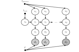
To invert sequential simulators, we define a probabilistic model over their parameters that encodes generic priors, and use approximate inference methods to infer probable values given data.
 |
1. = Initialize() and = Prob_Init(,) 2. = Sample() and = Prob_Smp(,) 3. = Simulate() and = Prob_Sim(,) 4. = Emit() and = Prob_Emt(,) 5. = Comp_Distance_Likelihood() |
We assume the simulator is Markovian; that is, at every time point , we have a state variable which only depends on the previous state and the parameter(s) for the state : and . For the initial state, we assume . Moreover, at every given the current state , an emission is generated from a distribution, . To afford the flexibility for many different forms of observable data, we allow simulators to come with arbitrary per-step likelihood terms. These terms are incorporated by defining a Bernoulli distribution with parameter , where is the real data and . We provide an example of the in Section 2.3.
2.1 Procedural interface for specifying sequential simulators
This probabilistic model lends itself to a natural software interface that can be satisfied by many sequential simulators:
-
1.
= Initialize() and = Prob_Init(,): These procedures return the state of the simulator at initialization and compute the probability of sampling state from the initializing distribution respectively.
-
2.
= Sample() and = Prob_Smp(,): These procedures sample the parameters for a time point and compute the probability of sampling.
-
3.
= Simulate() and = Prob_Sim(,): Given the current state of the simulator at time and the parameter(s) for that time point, these procedures return the next state and compute the probability of sampling.
-
4.
= Emit() and = Prob_Emit(,): Given the current state at time , these procedures emit the observation for that time point and computes the probability of emission.
-
5.
= Comp_Distance_Likelihood() : Given the observation and the real data, this procedure calculates the probability of having an observation at time .
2.2 A real-world example: inverting a geological forward model
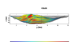
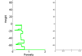
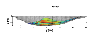
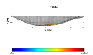
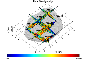
We focus on a simulator developed by an oil and gas company. In this model, the states () correspond to geological features called a lobes and the emissions () correspond to the porosities of the substrate. The parameters for each state are -tuples of independent uniform random variables, . The real data is given by a set of well logs, or sequences of porosities at varying heights, each at a different location in the geological model. Figure 6 shows a generated sample from the geological simulator. In our dataset, well logs are available for wells. The color of the lobe in renderings from the simulator represents the porosity at that lobe. See Figure 2 for a visualization of lobe formation and Figure 6 for the final output stratigraphy showing all 7 wells.
The simulator builds a lobe according to a complex geological model which given and is deterministic. The emission at a well location, denoted by , is a function of the current lobe and location . We assume the initial state is a function of a hyperparameter and the emissions at different locations are independent. For every emission 111To be more precise, every emission at well is a sequence of porosities indexed by height . The height at the end of lobe at well is denoted by ; hence, the generated observation at well and lobe is given by . Similarly, we can define the sequence of porosities for the real well logs., there will be a corresponding real well log for the same location and lobe . We set and .
The generative model for the observations at each lobe can be summarized as:
 |
 |
 |
 |
 |
 |
The problem of stochastic inversion of a sequential simulator is finding the joint posterior of the states and the parameters given a sequence of real data (i.e. finding in the model of Section 2). For the rest of this paper, we assume the model to be the geological model defined in this section.
2.3 Distance based likelihood function
In a complex simulator, the likelihood is intractable and an ABC filtering (Jasra et al., 2012) or ABC-MCMC (Marjoram et al., 2003) methods may be useful. However, in the geological model (without the distance based likelihood) and are delta distributions with a single atom. Thus, the likelihood is tractable. However, the deterministic structure of the simulator can result in poor performance of any inference method. For instance, in an SMC scheme, , which appears in the weight updating equations of particles, will be zero for all the particles with probability one. This explains the reason behind defining the likelihood in terms of the distance between the real data and the generated observation.
Recall that, for lobe and well , we denote the generated data by and the real data by . We assume that the error values for different locations are independent. For each location we use the following kernel to compute the error where is the parameter of the kernel which controls the bandwidth.
2.4 Probabilistic programming and automatic inference
We use Venture (Mansinghka et al., 2014) to represent our probabilistic model, including an interface to external simulation software. We use the automatic inference mechanisms in Venture to implement several strategies that can be applied to any simulator that satisfies the requirements of our interface. The Venture program we use for inverting all such simulators requires under 20 lines of probabilistic code.
Figure 3 shows the probabilistic code for the model and four inference strategies. We focus on inversion strategies built out of the building blocks provided by Metropolis Hastings (MH) and particle Markov chain Monte Carlo methods (PMCMC) (Andrieu et al., 2010). Each of the four strategies we present requires 4 or fewer lines of probabilistic code to implement. See (Mansinghka et al., 2014) for details regarding the syntax and semantics of Venture.
,gobble=-30, numbers=left,numbersep=2pt, frame=single, xleftmargin=10mm, xrightmargin = 0mm, fontsize=,,
[assume sim (make_simulator) ][assume get_init (lambda () (sim ’initialize)) ][assume get_params (mem (lambda (t) (scope_include 0 t (make_array (uniform_continuous 0 1) 5)))) ][assume get_state (mem (lambda (t) (sim ’simulate (get_params t) t (if (= t 0) (get_init) (get_state (- t 1))))))][assume get_emission (mem (lambda (t) (sim ’emit (get_state t)))))][assume get_distance (mem (lambda (t) (sim ’distance (get_emission t)))))]
,gobble=-30, numbers=left,numbersep=2pt, frame=single, xleftmargin=10mm, xrightmargin = -5mm, fontsize=, fontsize=,,
// Particle Gibbsfor t = 1...T: [observe (log_flip (get_distance t)) true][infer (pgibbs 0 ordered 10 50)]\KV@do,gobble=-30, numbers=left,numbersep=2pt, frame=single, xleftmargin=8mm, xrightmargin = 0mm, fontsize=, fontsize=,,
// Metropolis Hastingsfor t = 1...T: [observe (log_flip (get_distance t)) true][infer (mh default one 500)]
,gobble=-30, numbers=left,numbersep=2pt, frame=single, xleftmargin=10mm, xrightmargin = -5mm, fontsize=, fontsize=,,
// Hybrid PGibbs-MHfor t = 1...T: [observe (log_flip (get_distance t)) true][infer (cycle ((pgibbs 0 ordered 10 10) (mh default one 50)) 10)]
,gobble=-30, numbers=left,numbersep=2pt, frame=single, xleftmargin=8mm, xrightmargin = 0mm, fontsize=, fontsize=,,
// Sequential MHfor t = 1...T: [observe (log_flip (get_distance t)) true] for i == 1...t: [infer (mh 0 one 10)]
3 Experiments
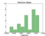
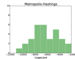
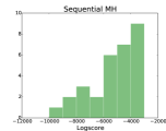
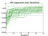
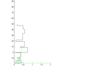
We report two experimental results. First, we compare the performance of particle Gibbs, Metropolis-Hastings and sequential Metropolis-Hastings. For all three methods, we set the kernel bandwidth to 1. We use 10 lobes; each of these problem instances involves exploring a jagged 50-dimensional energy landscape. Figure 4 shows the results. On this problem, we find sequential Metropolis-Hastings to be the most effective, with particle Gibbs also exhibiting reasonable performance. Pure Metropolis-Hastings occasionally performs quite well but exhibits higher variance, frequently getting stuck in local minima.
The three methods were run for roughly equivalent numbers of iterations (500), and their runtimes were all within a factor of 2 of each other. This is due to the runtime being dominated by calls to the simulator, and one iteration resulting in about 5-10 simulator calls for all three methods.
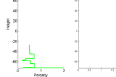
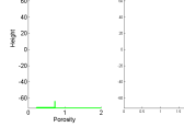
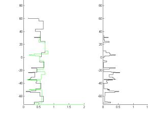
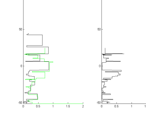
Figure 5 shows typical results for a larger-scale experiment searching over 80 lobes (400 dimensions). Many complex features of the well logs are captured by our method, although some wells are only poorly explained. Based on discussions with geologists, these results are comparable in quality to those obtained via a custom optimization-based baseline. It thus may be possible to improve accuracy as well as reduce code complexity by developing a more sophisticated inference scheme that can be automatically applied to this broad class of inversion problems.
 |
 |
 |
 |
 |
 |
 |
| (a) PGibbs - Well #4 | (b) PGibbs - Well #5 | (c) PGibbs - Well #6 |
4 Discussion
These preliminary results show that it is possible to use a general-purpose probabilistic programming system with only automatic, general-purpose inference mechanisms to invert sophisticated software simulators. A 10-line probabilistic program suffices. Multiple inference strategies can be specified with 4 or fewer lines, and can be compared to produce an ensemble of probable inversions. If the underlying simulator is changed, the only change to the probabilistic program that is needed is to generate the appropriate random parameters per simulation step. The inference programs do not need to be changed at all, even though the transition operators they induce may be quite different.
Future work will investigate more sophisticated models and automatic, general-purpose inference schemes, as well as applications to other simulators. It would be especially interesting to address statistical issues in inversion, for example by augmenting our simulator interface to expose and label parameters that affect model complexity or adjust the resolution of the data, and using model selection and parameter estimation to adjust them appropriately.
Acknowledgements
We thank Shell company for the funding and provision of the lobes forward stratigraphy simulator. We also thank Zoltan Sylvester, Alessandro Cantelli, Matt Wolinsky and Oriol Falivene who built the simulator code.
References
- Andrieu et al. (2003) Christophe Andrieu, Nando De Freitas, Arnaud Doucet, and Michael I Jordan. An introduction to mcmc for machine learning. Machine learning, 50(1-2):5–43, 2003.
- Andrieu et al. (2010) Christophe Andrieu, Arnaud Doucet, and Roman Holenstein. Particle markov chain monte carlo methods. Journal of the Royal Statistical Society: Series B (Statistical Methodology), 72(3):269–342, 2010.
- Boschetti et al. (1996) Fabio Boschetti, Mike C Dentith, and Ron D List. Inversion of seismic refraction data using genetic algorithms. Geophysics, 61(6):1715–1727, 1996.
- Calvet and Fisher (2007) Laurent E Calvet and Adlai J Fisher. Multifrequency news and stock returns. Journal of Financial Economics, 86(1):178–212, 2007.
- Chen et al. (2006) J Chen, Susan Hubbard, J Peterson, K Williams, M Fienen, P Jardine, and D Watson. Development of a joint hydrogeophysical inversion approach and application to a contaminated fractured aquifer. Water Resources Research, 42(6), 2006.
- Jasra et al. (2012) Ajay Jasra, Sumeetpal S Singh, James S Martin, and Emma McCoy. Filtering via approximate bayesian computation. Statistics and Computing, 22(6):1223–1237, 2012.
- Malinverno (2002) Alberto Malinverno. Parsimonious bayesian markov chain monte carlo inversion in a nonlinear geophysical problem. Geophysical Journal International, 151(3):675–688, 2002.
- Mansinghka et al. (2014) Vikash Mansinghka, Daniel Selsam, and Yura Perov. Venture: a higher-order probabilistic programming platform with programmable inference. ArXiv e-prints, March 2014.
- Marjoram et al. (2003) Paul Marjoram, John Molitor, Vincent Plagnol, and Simon Tavaré. Markov chain monte carlo without likelihoods. Proceedings of the National Academy of Sciences, 100(26):15324–15328, 2003.
- Ramillien (2001) Guillaume Ramillien. Genetic algorithms for geophysical parameter inversion from altimeter data. Geophysical Journal International, 147(2):393–402, 2001.
- Symes et al. (2011) William W Symes, Dong Sun, and Marco Enriquez. From modelling to inversion: designing a well-adapted simulator. Geophysical Prospecting, 59(5):814–833, 2011.