Efficient Iterative Processing
in the SciDB Parallel Array Engine

Abstract

Many scientific data-intensive applications perform iterative computations on array data. There exist multiple engines specialized for array processing. These engines efficiently support various types of operations, but none includes native support for iterative processing. In this paper, we develop a model for iterative array computations and a series of optimizations. We evaluate the benefits of an optimized, native support for iterative array processing on the SciDB engine and real workloads from the astronomy domain.

1 Introduction

Science is increasingly becoming data-driven [11]. From small research labs to large communities [31, 17], scientists have access to more data than ever before. As a result, scientists can increasingly benefit from using database management systems to organize and query their data [15, 30].

Scientific data often takes the form of multidimensional arrays (e.g., 2D images or 3D environment simulations). One approach to managing this type of array data is to build array libraries on top of relational engines, but many argue that simulating arrays on top of relations can be highly inefficient [4]. Scientists also need to perform a variety of operations on their array data such as feature extraction [14], smoothing [25], and cross-matching [23], which are not built-in operations in relational Database Management Systems (DBMSs). Those operations also impose different requirements than relational operators on a DBMS [6].

As a result, many data management systems are being built to support the array model natively [7, 25, 36]. Additionally, to handle today’s large-scale datasets, several engines, including SciDB [25], provide support for processing arrays in parallel in a shared-nothing cluster. Several benchmark studies have shown that these specialized array engines outperform both relational engines and MapReduce-type systems on a variety of array workloads [4, 33].

Many data analysis tasks today require iterative processing [8]: machine learning, model fitting, pattern discovery, flow simulations, cluster extraction, and more. As a result, most modern Big Data management and analytics systems (e.g., [16, 34]) support iterative processing as a first-class citizen and offer a variety of optimizations for these types of computations: caching [3], asynchronous processing [16], prioritized processing [20, 35], etc.

The need for efficient iterative computation extends to analysis executed on multi-dimensional scientific arrays. For example, astronomers typically apply an iterative outlier-removal algorithm to telescope images as one of the first data processing steps. Once the telescope images have been cleaned, the next processing step is to extract sources (i.e., stars, galaxies, and other celestial structures) from these images. The source extraction algorithm is most easily written as an iterative query as well. As a third example, the simple task of clustering data in a multi-dimensional array also requires iterating until convergence to the final set of clusters. We further describe these three applications in Section 2.

While it is possible to implement iterative array computations by repeatedly invoking array queries from a script, this approach is highly inefficient (as we show in Figure 10(a)). Instead, a large-scale array management systems such as SciDB should support iterative computations as first-class citizens in the same way other modern data management systems do for relational or graph data.

Contributions: In this paper, we introduce a new model for expressing iterative queries over arrays. We develop a middleware system called ArrayLoop that we implement on top of SciDB to translate queries expressed in this model into queries that can be executed in SciDB. Importantly, ArrayLoop includes three optimizations that trigger rewrites to the iterative queries and ensure their efficient evaluation. The first optimization also includes extensions to the SciDB storage manager. More specifically, the contribution of this paper are as follows:

(1) New model for iterative array processing (Sections 3 and 4): Iterating over arrays is different from iterating over relations. In the case of arrays, the iteration starts with an array and updates the cell values of that array. It does not generate new tuples as in a relational query. Additionally, these update operations typically operate on neighborhoods of cells. These two properties are the foundation of our new model for iterative array processing. Our model enables the declarative specification of iterative array computations, their automated optimization, and their efficient execution.

(2)Incremental iterative processing (Section 5): In many iterative applications, the result of the computation changes only partly from one iteration to the next. As such, implementations that recompute the entire result every time are known to be inefficient. The optimization, called incremental iterative processing [8], involves processing only the part of the data that changes across iterations. When this optimization is applicable, it has been shown to significantly improve performance in relational and graph systems [8, 20]. This optimization also applies to array iterations. While it is possible to manually write a set of queries that process the data incrementally, doing so is tedious, error-prone, and can miss optimization opportunities. Our iterative array model enables the automatic generation of such incremental computations from the user’s declarative specification of the overall iterative query. Additionally, while the idea of incremental iterations has previously been developed for relational systems, its implementation in an array engine is very different: For an array engine, the optimization can be pushed all the way to the storage manager with significant performance benefits. We develop and evaluate such storage-manager-based approach to incremental array processing.

(3) Overlap iterative processing (Section 6): In iterative array applications, including, for example, cluster finding and source detection, operations in the body of the loop update the value of the array cells by using the values of other neighboring array cells. These neighborhoods are often bounded in size. These applications can effectively be processed in parallel if the system partitions an array but also replicates a small amount of overlap cells. In the case of iterative processing, the key challenge lies in keeping these overlap cells up to date. This optimization is specific to queries over arrays and does not apply to relational engines. Our key contribution here lies in new mechanisms for managing the efficient reshuffling of the overlap data across iterations.

A subset of applications that leverage overlap data also have the property that overlap cells can be updated only every few iterations. Examples of such applications are those that try to find structures in the array data. They can find structures locally, and need to exchange information only periodically to stitch these local structures into larger ones. We extend our overlap data shuffling approach to leverage this property and further reduce the overhead of synchronizing overlap data. We call this optimization, mini-iterations.

(4)Multi-resolution iterative processing (Section 7): Finally, in many applications, the raw data lives in a continuous space (3D universe, 2D ocean, N-D space of continuous variables) and arrays capture discretized approximations of the real data. Different data resolutions are thus possible and scientifically meaningful to analyze. In fact, it is common for scientists to look at the data at different levels of detail. In many applications, it is often efficient to first process the low-resolution versions of the data and use the result to speed-up the processing of finer-resolution versions of the data if requested by the user. Our final optimization automates this approach. While scientists are accustomed to working with arrays at different levels or detail, our contribution is to show how this optimization can be automatically applied to iterative queries in an array engine.

(5) Implementation and evaluation We implement the iterative model and all three optimizations as extensions to the open-source SciDB engine and we demonstrate their effectiveness on experiments with 1 TB of publically-available synthetic LSST images [24]. Experiments show that Incremental iterative processing can boost performance by a factor of 4-6X compared to a non-incremental iterative computation. Iterative overlap processing together with mini-iteration processing can improve performance by 31% compare to SciDB’s current implementation of overlap processing. Finally, the multi-resolution optimization can cut runtimes in half if an application can leverage this technique. Interestingly, these three optimizations are complementary and their benefits can be compounded.

To the best of our knowledge, this paper is the first to design, implement, and evaluate an approach for iterative processing in a parallel array data management system. Given that array engines have been shown to outperform a variety of other systems on array workloads [4, 33] and that iterative analytics are common on array data (as we discussed above), efficient support for iterative query processing in array engines is a critical component of the big data engine ecosystem.

2 Motivating Applications

We start by presenting three array-oriented, iterative applications. We use these applications as examples throughout the paper and also in the evaluation.

Example 2.1.

Sigma-clipping and co-addition in LSST images (SigmaClip): The Large Synoptic Survey Telescope (LSST [17]) is a large-scale, multi-organization initiative to build a new telescope and use it to continuously survey the visible sky. The LSST will generate tens of TB of telescope images every night. Before the telescope produces its first images, astronomers are testing their data analysis pipelines using realistic but simulated images.

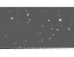
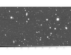
When analyzing telescope images, some sources (a “source" can be a galaxy, a star, etc.) are too faint to be detected in one image but can be detected by stacking multiple images from the same location on the sky. The pixel value (flux value) summation over all images is called image co-addition. Figure 1 shows a single image and the corresponding co-added image. Before the co-addition is applied, astronomers often run a “sigma-clipping" noise-reduction algorithm. The analysis in this case has two steps: (1) outlier filtering with “sigma-clipping" and then (2) image co-addition. Listing 1 shows the pseudocode for both steps. Sigma-clipping consists in grouping all pixels by their (x,y) coordinates. For each location, the algorithms computes the mean and standard deviation of the flux. It then sets to null all cell values that lie $k$ standard deviations away from the mean. The algorithm iterates by re-computing the mean and standard deviation. The cleaning process terminates once no new cell values are filtered out. Throughout the paper, we refer to this application as SigmaClip.  $\square$

Example 2.2.

Iterative source detection algorithm (SourceDetect): Once telescope images have been cleaned and co-added, the next step is typically to extract the actual sources from the images.

The pseudocode for a simple source detection algorithm is shown in Listing 2. Each non-empty cell is initialized with a unique label and is considered to be a different object. At each iteration, each cell resets its label to the minimum label value across its neighbors. Two cells are neighbors if they are adjacent. This procedure continues until the algorithm converges. We refer to this application as SourceDetect.  $\square$

Example 2.3.

K-means clustering algorithm (KMeans):  In many domains, clustering algorithms are commonly used to identify patterns in data. Their use extends to array data. We consider in particular K-means clustering on a 2D array [12]. K-means clustering works as follows: It assigns each cell randomly to one of the $k$ clusters. It computes the centroid of each cluster. It iterates by re-assigning each cell to its nearest cluster. We refer to this application as KMeans.  $\square$

These applications illustrate two important properties of iterative computations over arrays. First, the goal of an iterative computation is to take an array from an initial state to a final state by iteratively refining its content. The SigmaClip application, for example, starts with an initial 3D array containing 2D images taken at different times. Each iteration changes the cell values in this array. The iteration terminates when no cell changes across two iterations. Second, the value of each cell at the next iteration is determined by the values of a group of cells with some common characteristics at the current iteration. Those characteristics are often mathematically described for any given cell in the array. For SigmaClip those are “all pixel values at the same (x,y) location". Interestingly, unlike SigmaClip, where each group of cells at the same $(x,y)$ location influences many cell-values at the next iteration, in the SourceDetect algorithm any given cell $(x,y)$ is influenced by a unique group of cells, which are its adjacent neighbors. These groups of cells partially overlap with each other, which complicates parallel processing as we discuss in Section 6.

(a) Single image

(b) Co-added image

Figure 1: Illustrative comparison of a single telescope image and its corresponding co-added image. Many faint objects become visible after co-addition.

Input: Array A with pixels from x-y images over time.
//Part 1: Iterative sigma-clipping
While(some pixel changes in A)
 For each (x,y) location
  Compute mean/stddev of all pixel values at (x,y).
  Filter any pixel value that is k
  standard deviations away from the mean
//Part 2: Image co-addition
Sum all non-null pixel values grouped by x-y

Listing 1 Pseudocode for SigmaClip application

Input: Co-added Array A with uniquely labeled pixels from
       all the x-y images.
Input: int r, the adjacency threshold.
While(some pixel changes in A)
 For each (x,y) location
  Compute the minimum label of all pixel values (x’,y’)
  with x-r <= x’<= x+r  and  y-r <= y’<= y+r.
  Update (x,y) with the minimum label.

Listing 2 Pseudocode for SourceDetect application

3 Iterative Array-Processing Model

We start with a formal definition of an array similar to Furtado and Baumann [9]: Given a discrete coordinate set $S=S_{1}\times\ldots\times S_{d}$, where each $S_{i},i\in[1,d]$ is a finite totally ordered discrete set, an array is defined by a d-dimensional domain $D=[I_{1},\ldots,I_{d}]$, where each $I_{i}$ is a subinterval of the corresponding $S_{i}$. Each combination of dimension values in D defines a cell. All cells in a given array $A$ have the same type $T$, which is a tuple. $cells(A)$ is the set of all the cells in array $A$ and function $V:cells(A)\rightarrow T$ maps each cell in array $A$ to its corresponding tuple with type $T$. In the rest of the paper, we refer to the dimension $x$ in array $A$ as $A[x]$ and to each attribute $y$ in the array $A$ as $A.y$.

Figure 2: Iterative array $A$ and its state at each iteration for the SourceDetect application. $\{Q^{f^{\pi},\delta^{\pi}}_{cells(A)}:\forall c_{i,j}\in cells(A)\;i\in I_{1}\;\&\;j\in I_{2}\;\}$ where $I_{1}=I_{2}=\{1,2,3,4\}$ are the sets of dimension values, $f^{\pi}$ applies $min()$ aggregate on each group of cells, $\delta^{\pi}$ simply stores the aggregated value in each cell $c_{i,j}$, and $\pi:(x,y)\rightarrow[x\pm 1][y\pm 1]$. At each iteration, a sliding window scans through all the cells.

In SciDB, users operate on arrays by issuing declarative queries using either the Array Query Language (AQL) or the Array Functional Language (AFL). The select statements in Algorithm 1 in Section 5 are examples AQL queries. AQL and AFL queries are translated into query plans in the form of trees of array operators. Each operator $O$ takes one or more arrays as input and outputs an array: $O:A\rightarrow A$ or $O:A\times A\rightarrow A$.

In an iterative computation, the goal is to start with an initial array $A$ and transform it through a series of operations in an iterative fashion until a termination condition is satisfied. The iterative computation on $A$ typically involves other arrays, including arrays that capture various intermediate results (e.g., arrays containing the average and standard deviation for each $(x,y)$ location in the SigmaClip application) and arrays with constant values (e.g., a connectivity matrix in a graph application).

One can use the basic array model to express iterative computations. The body of the loop can simply take the form of a series of AQL or AFL queries. Similarly, the termination condition can be an AQL or AFL query. In Section 5, the first function in Algorithm 1 illustrates this approach.

To enable optimizations, however, we extend the basic array model with constructs that capture in greater details how iterative applications process arrays. We start with some definitions.

Definition 3.1.

We call an array iterative if its cell-values are updated during the course of an iterative computation. The array starts with an initial state $A_{0}$. As the iterative computation progresses, the array goes through a set of states $A_{1}$, $A_{2}$, $A_{3}$, $\ldots$, until a final state $A_{N}$. Note that all $A_{i}$ have the same schema. In other words, the shape of an iterative array does not change.

Figure 2 shows a (4$\times$4) iterative array that represents a tiny telescope image in the SourceDetect application. In the initial state, $A_{0}$, each pixel with a flux value above a threshold is assigned a unique value. As the iterative computation progresses, adjacent pixels are re-labeled as they are found to belong to the same source. In the final state $A_{3}$, each set of pixels with the same label corresponds to one detected source.

Iterative applications typically define a termination condition that examines the cell-values of the iterative array:

Definition 3.2.

An iterative array $A$ has converged, whenever $T(A_{i},A_{i+1})\leq\epsilon$ for some aggregate function $T$. $T$ is the termination condition. $\epsilon$ is a user-specified constant.

In Figure 2, convergence occurs at iteration 3 when $\epsilon=0$ and the termination condition $T$ is the count of differences between $A_{i}$ and $A_{i+1}$. Our ArrayLoop system represents $T$ as AQL function.

An iterative array computation takes an iterative array, $A$, and applies to it a computation $Q$ until convergence:

$$A_{0}\xrightarrow{Q}A_{1}\xrightarrow{Q}\dots\xrightarrow{Q}A_{i}\xrightarrow{Q}A_{i+1}$$ (1)

where $Q$ is a sequence of valid AQL or AFL queries. At each step, $Q$ can either update the entire array or only some subset of the array. We capture the distinction with the notion of major and minor iteration steps:

Definition 3.3.

A state transition, $A_{i}\xrightarrow{Q}A_{i+1}$, is a major step if the function $Q$ operates on all the cells in $A$ at the same time. Otherwise it is a minor step.

The array state $A_{i,j}$ represents the state of the iterative array after $i$ major steps followed by $j$ minor steps. We are interested in modeling computations where each major step can be decomposed into a set of minor steps that can be evaluated in parallel. That is, a major step $Q_{i}$ can be expressed as a set of minor steps $q_{i}$ such that $\sigma$, $Q_{i}=q_{i,\sigma_{1}}\cdot q_{i,\sigma_{2}}\dots q_{i,\sigma_{n-1}}\cdot q_{i,\sigma_{n}}$.

The iterative array computation in Equation 2 includes $(i+1)$ major steps. The first line illustrates the transition of iterative array $A$ in major steps and the second line illustrates the possible minor steps that can replace the major step $Q_{i+1}$. A termination condition check always occurs between two states of an iterative array after a major step.

$$A_{0}\xrightarrow{Q_{1}}A_{1}\xrightarrow{Q_{2}}\dots A_{i-1}\xrightarrow{Q_{i}}A_{i}\xrightarrow{Q_{i+1}}A_{i+1}$$ (2)

$$\overbrace{A_{i}\xrightarrow{q_{i,1}\cdot q_{i,2}\dots q_{i,j-1}\cdot q_{i,j}}A_{i+1}}$$

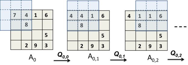
Figure 2 shows an iterative array computation with only major steps involved, while Figure 3 presents the same application but executed with minor steps.

Figure 3: Iterative array $A$ and its state after three minor steps, each of the form: $Q_{i,j}=Q^{f^{\pi},\delta^{\pi}}_{c_{i,j}}$ where $c_{i,j}$ is the cell at $A[i][j]$, $f^{\pi}$ applies $min()$ aggregate, $\delta$ simply stores the aggregate result as the new value in cell $c_{i,j}$, and $\pi:(x,y)\rightarrow[x\pm 1][y\pm 1]$

We further observe from the example applications in Section 2 that the functions $Q$ often follow a similar pattern.

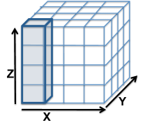
First, the value of each cell in iterative array $A_{i+1}$ that is updated by $Q$ only depends on values in nearby cells in array $A_{i}$. We capture this spatial constraint with a function $\pi$ that specifies the mapping from output cells back onto input cells:

Definition 3.4.

$\pi$ is an assignment function defined as $\pi:cells(A)\rightarrow\mathcal{P}\left(cells(A)\right)$, where $cells(A)$ is the set of all the cells in array $A$ and $\mathcal{P}()$ is the powerset function.

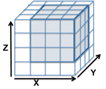
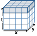
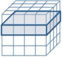
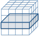
Figure 4 illustrates two examples of assignment functions. Our ArrayLoop system supports two types of assignment functions: windowed functions such as those illustrated in Figure 4 and attribute assignment function. The latter occur in applications such as K-means clustering described in Example 2.3: $\pi:(x,y)\rightarrow label$ where all the cells with the same label are grouped together.

Definition 3.5.

$f^{\pi}$ is an aggregate function defined as $f^{\pi}:cells(A)\rightarrow\tau$. $f^{\pi}$ groups the cells of the array $A$ according to assignment function $\pi$, with one group of cells per cell in the array $A$. It then computes the aggregate functions separately for each group. The aggregate result is stored in tuple $\tau$.

Finally, $Q$ updates the output array with the computed aggregate values:

Definition 3.6.

$\delta^{\pi}:(cells(A),f^{\pi})\rightarrow cells(A)$ is a cell-update function. It updates each cell of the array $A$ with the corresponding tuple $\tau$ computed by $f^{\pi}$ and the current value of the cell itself.

These three pieces together define the iterative array computation $Q^{f^{\pi},\delta^{\pi}}_{C}$ as follows:

Definition 3.7.

An iterative array computation $Q^{f^{\pi},\delta^{\pi}}_{C}$ on the subset of cells $C$ where $C\in\mathcal{P}(cells(A))$ generates subset of cells $C^{{}^{\prime}}\in\mathcal{P}(cells(A))$ such that $\forall c\in C$ and $c^{{}^{\prime}}\in C^{{}^{\prime}}$ $c^{{}^{\prime}}=\delta^{\pi}(c,f^{\pi}(c))$ where $c$ and $c^{{}^{\prime}}$ are two corresponding cells in those subsets.

In the example from Figures 2 and 3, which illustrate the SourceDetect application, the goal is to detect all the clusters in the array $A$, where each cell $p_{1}=(x_{1},y_{1})$ in a cluster has at least one neighbor $p_{2}=(x_{2},y_{2})$ in the same cluster such that $|x_{1}-x_{2}|\leq 1$ and $|y_{1}-y_{2}|\leq 1$, if it is not a single-cell cluster. In this application, $\pi$ is the 3X3 window around a cell. We slide the window over the array cells in major order. At each minor step, at each cell $c_{i,j}$ at the center of the window, we apply an iterative array computation $Q_{i,j}=Q^{f^{\pi},\delta^{\pi}}_{c_{i,j}}$ where $f^{\pi}$ applies a $min()$ aggregate over the 3x3 window, $\pi$, and $\delta^{\pi}$ is a cell-update function that simply stores the result of the $min()$ aggregate into cell $c_{i,j}$. Figure 3 illustrates three steps of this computation. Notice that the output of the iterative array computation $Q_{0,0}$ becomes the input for $Q_{0,1}$ and so on. Another strategy is to have many windows grouped and applied together. In other words, instead of applying the iterative array computation per cell, we apply $Q^{f^{\pi},\delta^{\pi}}_{C}$ on a group of cells $C\in\mathcal{P}\left(cells(A)\right)$ in one major step. Note that when using minor steps, the output of each minor step serves as input to the next step. In contrast, when using major steps, the iterative array computations see the original array state at the beginning of that iteration. Figure 2 shows the iterative array computation for the latter strategy. The former strategy has less expensive steps than the latter strategy, but it requires more steps to converge.

(a) SourceDetect

(b) SigmaClip

Figure 4: Two examples of window assignment functions: (a) $\pi_{1}:(x,y,z)\rightarrow[x\pm 1][y\pm 1][z\pm 1]$, the associated window is highlighted for the cell at $(2,1,2)$. (b) $\pi_{2}:(x,y,z)\rightarrow[x][y]$, the associated window is highlighted for all the cells at $(x,y,z)$ with $z=0$.

In our model, we encapsulate all the elements of the model in a FixPoint operator:

$$FixPoint(A,\pi,f,\delta,T,\epsilon)$$ (3)

With our model, the user specifies the logic of the iterative algorithm without worrying about the way it is going to be executed. Our model can be implemented and executed on top of various array execution engines. In the rest of the paper, we describe how the queries specified in our model are rewritten and efficiently run in the SciDB array engine. The execution strategy in SciDB uses only major steps. Mini-step iterations, i.e. asynchronous execution, is left for future study.

4 Iterative Array Processing

We extend SciDB-Py [27] with a python $FixPoint()$ operator following the model from Section 3. We also develop an optimizer module that we name ArrayLoop. The user encapsulates its iterative algorithm in the $FixPoint()$ operator. The ArrayLoop optimizer sits on top of SciDB. ArrayLoop rewrites a $FixPoint(A,\pi,f,\delta,T,\epsilon)$ operator into the AQL queries in Listing 3 that it wraps with an internal while loop.

is_window helper function in Listing 3 clarifies whether the window assignment function translates to a window aggregate or a group-by aggregate. ArrayLoop translates a window assignment function to a group-by aggregate if mapping is from a set of input dimensions to one of its subsets. If mapping is from a set of dimensions to the same set of dimensions with additional offsets per dimension, then ArrayLoop translates it to window-aggregate. Supporting window assignment function that is a combination of group-by aggregate and window aggregate is left for future work.

In addition, ArrayLoop also implements a set of query re-writing tasks in order to leverage a series of optimizations that we develop: incremental iterative processing, overlap iterative processing, and multi-resolution iterative processing.

Input:
  FixPoint(A,pi,f,delta,T,epsilon)
Output:
  While (T(A,A_prev)  < epsilon)
   // Termination function T is also AQL function.
   // Compute the new aggregates from the current iterative array.
   If (is_window(pi))
      G = SELECT f FROM A WINDOW PARTITIONED BY pi
   else
      G = SELECT f FROM A GROUP BY pi
   // Combine the new aggregate with the old value of the cell.
   S = SELECT * FROM G JOIN A ON <matching dimensions>
   A_new = SELECT delta(S) FROM S
   A_prev = A
   A = A_new

Listing 3 Pseudocode for rewriting FixPoint operator

ArrayLoop acts as a pre-processing module before executing the iterative query in SciDB. Currently the majority of the ArrayLoop implementation is outside the core SciDB engine. As future work, we are planning to push the ArrayLoop python prototype into the core SciDB engine. ArrayLoop relies on SciDB for features such as distributed query processing, fault-tolerance, data distribution, and load balancing. In the following sections, we describe each of the three optimizations in more detail.

5 Incremental Iterations

Algorithm 1 SigmaClip application followed by image co-addition

1.function sigma-clipping($A$,$k$) $\triangleright$ Naïve sigma-clip

2. Input: Iterative Array $A$ $<$float $d$$>$[$x$,$y$,$t$]

3. Input: $k$ a constant parameter.

4. while (some pixels $A[x,y,t]$ are filtered) do

5.   $T[x,y]$ = select $avg(d)$ as $\mu$, $stdv(d)$ as $\sigma$ from $A$ group by $x,y$

6.   $S[x,y,t]$ = select * from $T$ join $A$ on $T.x$ = $A.x\;and\;T.y$=$A.y$

7.   $A[x,y,t]$ = select $d$ from $S$ where $\mu-k\times\sigma\leq d\leq\mu+k\times\sigma$

8. end while

9.end function

10.

11.function incr-sigma-clipping($A$,$k$) $\triangleright$ Incremental sigma-clip

12. Input: Array $A$ $<$float $d$$>$[$x$,$y$,$t$].

13. Input: $k$: a constant parameter.

14. Local: Array $C$ $<$int $c$,float $s$,float $s^{2}$$>$[$x$,$y$].

15. Local: $Collect\leftarrow\phi$ $\triangleright$ Collects all the filtered points.

16. Local: $Remain\leftarrow A$ $\triangleright$ Keeps track of remaining points.

17. $\Delta A\leftarrow A$

18. while ($\Delta A$ is not empty) do

19.   $T_{1}[x,y]\leftarrow$ select count$(d)$ as $c$, sum($d$) as $s$, sum($d^{2}$) as $s^{2}$ from $\Delta A$ group by $x,y$

20.  if (first iteration) then

21.   $C\leftarrow T_{1}[x,y]$

22.  else

23.    $\Delta$C[x,y] $\leftarrow$ select $C.c-T_{1}.c$ as $c$ , $C.s-T_{1}.s$ as $s$ , $C.s^{2}-T_{1}.s^{2}$ as $s^{2}$ from $C$ join $T_{1}$ on $T_{1}.x$ = $C.x\;\&\;T_{1}.y$=$C.y$

24.  end if

25.   $T[x,y]\leftarrow$ select $\frac{C.s}{C.c}$ AS $\mu$, $\sqrt[2]{\frac{C.s^{2}}{C.c}-(\frac{C.s}{C.c})^{2}}$ AS $\sigma$ from $\Delta C$

26.   $S[x,y,t]\leftarrow$ select $A.d$, $T.\mu$, $T.\sigma$ from $T$ join $Remain$ on $T.x$ = $A.x\;\ and\;T.y$=$A.y$

27.   $\Delta A\leftarrow$ select $d$ from $S$ where $d\leq\mu-k\times\sigma\;or\;d\geq\mu+k\times\sigma$

28.  $Remain\leftarrow\pi_{d}(S)$-$\Delta A$ $\triangleright$ Updates Remain.

29.  $Collect\leftarrow$ $\Delta A$ $\triangleright$ Adds the filtered points to Collect.

30. end while

31. $A\leftarrow A$-$Collect$$\triangleright$ Produces the final state for A.

32.end function

33.

34.co-addition phase:

35.$R[x,y]\leftarrow$ select sum($A.d$) as $coadd$ from $A$ group by $x,y$

Figure 5: Snapshots from the first 3 iterations of the SigmaClip application with the incremental-processing optimization on the LSST dataset. Green-colored points are the ones that change across iterations. (a) Original Image (b) Iteration-1 (c) Iteration-2 (d) Iteration-3.

Algorithm 2 ArrayLoop version of the SigmaClip application followed by image co-addition

1.function ArrayLoop-sigma-clipping($A$,$k$) $\triangleright$ SigmaClip algorithm with FixPoint operator provided by the user.

2. Input: Iterative Array $A$ $<$float $d$$>$[$x$,$y$,$t$],

3. Input: $k$ a constant parameter.

4. $\pi:[x][y][z]\rightarrow[x][y].$

5. $\delta:``A.d\geq\mu-k\times\sigma$ and $A.d\leq\mu+k\times\sigma?A:null"$

6. $f:\{avg()\;as\;\mu,stdv()\;as\;\sigma\}$

7. $FixPoint(A,\pi,f,\delta,count(),0)$

8.end function

9.

10.function ArrayLoop-incr-sigma-clipping($A$,$k$) $\triangleright$ ArrayLoop incremental rewriting of the SigmaClip.

11. Input: Iterative Array $A$ $<$float $d$$>$[$x$,$y$,$t$],

12. Input: $k$: a constant parameter.

13. Local: Iterative Array $C$ $<$int $c$,float $s$,float $s^{2}$$>$[$x$,$y$],

14. Local: Array $S$ $<$float $\sigma$,float $\mu$$>$[$x$,$y$],

15. $\Delta A^{-}\leftarrow A$

16. while ($\Delta A^{-}$ is not empty) do

17.   $T[x,y]\leftarrow$ select count$(d)$ as $c$, sum($d$) as $s$, sum($d^{2}$) as $s^{2}$ from $\Delta A^{-}$ group by $x,y$

18.  if (first iteration) then

19.   $C\leftarrow T[x,y]$

20.  else

21.   merge($C$,$T$,$C.c-T.c$)

22.   merge($C$,$T$,$C.s-T.s$)

23.   merge($C$,$T$,$C.s^{2}-T.s^{2}$)

24.  end if

25.   $S[x,y]\leftarrow$ select $\frac{T.s}{T.c}$ AS $\mu$, $\sqrt[2]{\frac{T.s^{2}}{T.c}-(\frac{T.s}{T.c})^{2}}$ AS $\sigma$ FROM $\Delta^{+}C$

26.  merge$(A,S,S.\mu-k\times S.\sigma\leq A.d\leq S.\mu+k\times S.\sigma?A:null)$

27. end while

28.end function

29.co-addition phase:

30.$R[x,y]\leftarrow$ select sum($A.d$) as $coadd$ from $A$ group by $x,y$

In a wide range of iterative algorithms, the output at each iteration differs only partly from the output at the previous iteration. Performance can thus significantly improve if the system computes, at each iteration, only the part of the output that changes rather than re-computing the entire result every time. This optimization called incremental iterative processing [8] is well-known, e.g.  in semi-naive datalog evaluation, and has been shown to significantly improve performance in relational and graph systems. ArrayLoop leverages the iterative computation model from Section 3 to automatically apply this optimization when the semantics of the applications permit it. The SigmaClip application described in Section 2.1 is an example application that can benefit from incremental iterative processing. Figure 5 shows multiple snapshots of running the sigma-clipping algorithm using incremental iterative processing, on a subset of the lsst dataset. Green-colored points are the ones with changed values across two consecutive iterations. As the iterative computation proceeds, the number of green-colored points drops dramatically and consequently the amount of required computation at that step.

sigma-clipping() and incr-sigma-clipping() modules in Algorithm 1 show the original implementation and the manually-written incremental version of the implementation, respectively. In the sigma-clipping() module, the avg() and stdv() aggregate operators are computed over the whole input at each iteration, which is inefficient. In incr-sigma-clipping(), the user rewrites the avg() and stdv() aggregate operators in terms of two other aggregate operators count() and sum() (Algorithm 1, Lines 19 and 25). The user also needs to carefully merge the current partial aggregates with the aggregate result of the previous iteration (Algorithm 1, Line 23). As shown in Algorithm 1, writing an efficient incremental implementation is not a trivial task. It is painful for users if they need to rewrite their algorithms to compute these increments and manage them during the computation. Ideally, the user wants to define the semantics of the algorithm and the system should automatically generate an optimized, incremental implementation. Additionally, as we show in the evaluation, if the system is aware of the incremental processing, it can further optimize the implementation by pushing certain optimizations all the way to the storage layer.

5.1 Rewrite for Incremental Processing

In ArrayLoop, we show how the incremental processing optimization can be applied to arrays. As shown in Algorithm 2, with ArrayLoop, the user provides a FixPoint operator in ArrayLoop-sigma-clipping function. ArrayLoop automatically expands and rewrites the operation into an incremental implementation as shown in the ArrayLoop-incr-sigma-clipping function. The rewrite proceeds as follows. If the aggregate function $f$ is incremental, ArrayLoop replaces the initial aggregation with one over Delta A- or Delta A+ or both. For example, for ArrayLoop-incr-sigma-clipping, only negative delta arrays are generated at each iteration(there is no $\Delta A^{+}$). So the rewrite produces a group-by aggregate only on $\Delta A^{-}$ (line 16). Next, ArrayLoop merges the partial aggregate values with the aggregate results from the previous iteration (lines 20 through 22). The aggregate rewrite rules define that merge logic for all the aggregate functions. In this example, ArrayLoop will generate one merge statement per aggregate function computed earlier. Finally, on Line 24, ArrayLoop does the final computation to generate the final aggregate values for this iteration. Note that finalize phase in the aggregate computation is always done on positive delta arrays ($\Delta C^{+}$), which generates the same result as computing on negative delta array $\Delta C^{-}$ followed by a subtract merge plus computing on positive delta array $\Delta C^{+}$ followed by an addition merge. Line 25 leverages the $\delta$ function to generate the $\Delta A^{-}$ of the next iteration.

Currently the decision whether the application semantics permit incremental iterative processing is left to the user. Given the FixPoint operator, ArrayLoop performs two tasks: (1) it automatically rewrites aggregate functions, if possible, into incremental ones and (2) it efficiently computes the last state of the iterative array using the updated cells at each iteration. The automatic rewrite is enabled by the precise model for iterative computations in the form of the three functions $\pi$, $f$, and $\delta$. Given this precise specification of the loop body, ArrayLoop rewrites the computation using a set of rules that specify how to replace aggregates with their incremental counter-parts when possible. To efficiently compute incremental state updates, we introduce a special merge operator. We now describe both components of the approach.

(1) Automatic aggregate rewrite: ArrayLoop triggers the incremental iterative processing optimization if any aggregate function in the FixPoint operator is flagged as incremental. The Data cube paper [10] defines an aggregate function $F()$ as algebraic if there is an M-tuple valued function $G()$ and a function $H()$ such that: $F(\{X_{i,j}\})=H(\{G(\{X_{i,j}\}|i=1,\dots,I\})|j=1,\dots,J\})$. ArrayLoop stores a triple $(agg,\{G_{1},\dots,G_{k}\},H)$ for any $algebraic$ function in the system and rewrites the aggregate query in terms of $G()$ and $H()$ functions during the query rewriting phase. For example, ArrayLoop records the triple (avg(),{sum(),count()},sum/count) and rewrites the algebraic average function avg() using the combination of sum() and count() to leverage incremental iterative processing.

(2) Incremental state management: ArrayLoop provides an efficient method for managing array state and incremental array updates during the course of an iterative computation. We observe that, during incremental processing, a common operation is to merge the data in two arrays, which do not necessarily have the same number of dimensions. In our example application, merging happens when the partial aggregates are combined with the aggregate result of the previous iteration, line 23 in incr-sigma-clipping() function. This operation merges together two 2D arrays where the merge logic is inferred from the incremental aggregate function $f$. Such merging also happens when the results of the aggregate function are used to update the iterative array, lines 26 and 27 in incr-sigma-clipping() function. In this case, the application merges the data in a 2D array with the data in a 3D array by sliding or extruding the 2D array through the 3D array. The $\delta$ cell-update function defines the logic of the merge operation in this case. The $\pi$ assignment function pairs-up cells from the intermediate aggregation array and the iterative array that merge together and thus determines whether merging will occur between arrays with the same number of dimensions or not.

In the manual implementation, shown in the incr-sigma-clipping() function, the user implements the merge logic manually using join and filter queries, which is inefficient. To remove this inefficiency, given the FixPoint operator, ArrayLoop automatically generates queries with explicit merge points that leverage a new merge operator that we add to SciDB: merge(Array source, Array extrusion, Expression exp).

The new merge operator is unique in a sense that it not only specifies the merge logic between two cells via a mathematical expression, exp, but it also automatically figures out which pairs of cells from the two arrays merge together by examining their common dimensions. ArrayLoop merges two cells from the source array and extrusion array if they share the same dimension-values in those dimensions that match in dimension-name. One cell in the extrusion array can thus merge with many cells in the source array. Figure 6 illustrates the merge operator for queries in lines 26 and 27 in Algorithm 1. As the figure shows, the extrusion array slides through the source array as the merging proceeds.

5.2 Pushing Incremental Computation into the Storage Manager

We observe that increments between iterations translate into updates to array cells and can thus be captured with two auxiliary arrays: a positive delta array and a negative delta array. At each iteration, the positive delta array $\Delta A^{+}$ records the new values of updated cells and the negative delta array $\Delta A^{-}$ keeps track of the old values of updated cells. Delta arrays can automatically be computed by the system directly at the storage manager level.

As a further optimization, we extend the SciDB storage manager to manage simple merge operations such as addition/subtraction found in Lines 21, 22, and 23 of Algorithm 2. ArrayLoop uses naming conventions as a hint to the storage manager about the semantics of the merge operation. For example $A_{(-)}\leftarrow B$, asks the storage manager to subtract array $B$ from array $A$ and store the result of the $(A-B)$ operation as the new version of array $A$. In case array $A$ is iterative, the new values and the old values of updated cells are stored in $\Delta^{+}A$ and $\Delta^{-}A$, respectively.

Typically, the user need not worry about these annotations and processing details since ArrayLoop automatically generates the appropriate queries from the FixPoint specification. However, the user can leverage these optimizations manually as well. For example, the queries in the incr-sigma-clipping() function at Lines 28, 29, and 31 (queries with red box frames) can all be pushed into the storage manager.

To achieve high performance, the storage manager keeps chunks of the result array $A$ together on disk with the corresponding chunks from the auxiliary $\Delta A^{+}$ and $\Delta A^{-}$ arrays. As we showed in previous work on array versioning [32], the space overhead of delta arrays taken between similar array versions is typically insignificant compared with the size of the original array.

We extend the Scan() and Store() operators to read and write partial arrays $\Delta A^{+}$ and $\Delta A^{-}$, respectively. With those optimizations, the user does not need to explicitly write a user-defined diff() function or, as shown in the incr-sigma-clipping() example, a sequence of join() and filter() queries in order to extract delta arrays from the output of the last iteration.

In prior work [22], we demonstrated a prototype implementation of the SigmaClip application together with the incremental iterative processing optimizations in the context of the AscotDB system that we built. AscotDB results from the integration of ASCOT, a Web-based tool for the collaborative analysis of telescope images and their metadata, and SciDB, a parallel array processing engine. The focus of the demonstration was on this system integration and on the impact of the optimizations on the application. AscotDB shows that average users who use graphical interfaces to specify their analysis also benefit from optimized iterative processing provided by lower layers of the analysis stack.

(a) step 1

(b) step 2

(c) step 3

(d) step 4

Figure 6: merge$(A,T,T.\mu-k\times T.\sigma\leq A.d\leq T.\mu+k\times T.\sigma?A:null)$ in SigmaClip application. This is the core filtering step where the outliers are removed. The 3D source array $A$ $<$float $d$$>$[$x$,$y$,$t$] and the 2D extrusion array (highlighted) $T$ $<$float $\mu$,float $\sigma$$>$[$x$,$y$] share the first two dimensions. (a), (b), (c), and (d) show how the cells in the extrusion array slide into the source array at runtime.

6 Iterative Overlap Processing

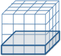
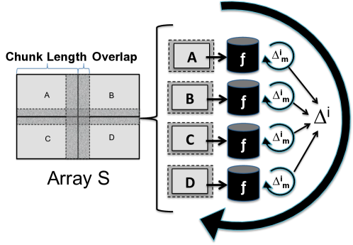
To process a query over a large-scale array in parallel, SciDB (and other engines) break arrays into sub-arrays called chunks, distribute chunks to different compute nodes (each node receives multiple chunks), and process chunks in parallel at these nodes. For many operations, such as filter for example, one can process chunks independently of each other and can union the result. This simple strategy, however, does not work for many scientific array operations. Frequently, the value of each output array cell is based on a neighborhood of input array cells. Data clustering is one example. Clusters can be arbitrarily large and can go across array chunk boundaries. A common approach to computing such operations in parallel is to perform them in two steps: a local, parallel step followed by an aggregate-type post-processing step [13, 14, 18] that merges partial results into a final output. For the clustering example, the first step finds clusters in each chunk. The second step combines clusters that cross chunk boundaries [13]. Such a post-processing phase, however, can add significant overhead. To avoid a post-processing phase, some have suggested to extract, for each array chunk, an overlap area $\epsilon$ from neighboring chunks, store the overlap together with the original chunk [25, 28], and provide both the core data and overlap data to the operator during processing [6]. This technique is called overlap processing. Figure 7 shows an example of array chunks with overlap. We refer the interested reader to our ArrayStore paper [6] for a more detailed discussion of efficient overlap processing techniques. These techniques, however, do not address the question of how best to update the overlap data during an iterative computation. Our contribution in this paper is to tackle this specific question.

6.1 Efficient Overlap Processing

Array applications that can benefit from overlap processing techniques are those that update the value of certain array cells by using the values of neighboring array cells. The SourceDetect application described in Section 2.2 is an example application that can benefit form overlap processing. Other example applications include “oceanography particle tracking”, which follow a set of particles as they move in a 2D or 3D grid. A velocity vector is associated with each cell in the grid and the goal is to find a set of trajectories, one for each particle in the array. Particles cannot move more than a certain maximum distance (depending on the maximum velocity of particles) at each step. These applications can be effectively processed in parallel by leveraging overlap processing techniques.

The challenge, however, is to keep replicated overlap cells up-to-date as their values change across iterations. To efficiently update overlap array cells, we leverage SciDB’s bulk data-shuffling operators as follows: SciDB’s operator framework implements a bool requiresRepart() function that helps the optimizer to decide whether the input array requires repartitioning before the operator actually executes. The partitioning strategy is determined by the operator semantics. For example, WindowAggregate operator [26] in SciDB requires repartitioning with overlap in case the input array is not already partitioned in that manner. We extend the SciDB operator interface such that ArrayLoop can dynamically set the returned value of the operator’s requiresRepart() function. To update overlap data, ArrayLoop sets the requiresRepart() return value to true. ArrayLoop has the flexiblity to set the value to true either at each iteration or every few iterations as we discuss further below. In case an operator in SciDB is guided by ArrayLoop to request repartitioning, the SciDB optimizer injects the Scatter/Gather [26] operators to shuffle the data in the input iterative array before the operator executes.

A benefit of using SciDB’s existing Scatter/Gather operators, is that they shuffle array data one chunk (i.e., sub-array) at a time. Chunk-based data shuffling is faster compared with the method that shuffles overlap data one cell at a time. The downside of using SciDB’s Scatter/Gather general operators is the relative higher cost of data shuffling when only a few overlap cells have changed.

6.2 Mini-Iteration Processing

Keeping overlap cells updated at each iteration requires reading data from disk, shuffling it across the network, and writing it to disk. These are all expensive operations. Any reduction in the number of such data synchronization steps can yield significant performance improvements.

We observe that a large subset of iterative applications have the property that overlap cells can be updated only every few iterations. These are applications, for example, that try to find structures in the array data, e.g. SourceDetect application. These applications can find structures locally and eventually need to exchange information to stitch these local structures into larger ones. For those applications, ArrayLoop can add the following additional optimization: ArrayLoop runs the algorithm for multiple iterations without updating the replicas of overlap cells. The application iterates over chunks locally and independently of other chunks. Every few iterations, ArrayLoop triggers the update of overlap cells, and continues with another set of local iterations. The key idea behind this approach is to avoid data movement across array chunks unless a large enough amount of change justifies the cost.

We call each series of local iterations without overlap cell synchronization mini iterations. Figure 7 illustrates the schematic of the mini iteration optimization.

An alternative approach is for the scheduler to delegate the decision to shuffle overlap data to individual chunks, rather than making the decision array-global as we do in this paper. We leave this extra optimization for future work.

Figure 7: Illustration of the mini-iteration optimization. $\Delta^{i}_{m}$ represents local changes at iteration $i$ of mini-iteration $m$ and $\Delta^{i}$ is the global change at iteration $i$.

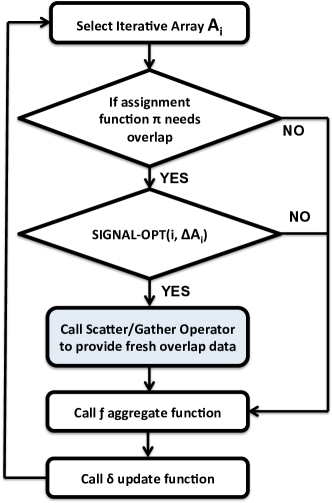
ArrayLoop includes a system-configurable function SIGNAL-OPT() that takes as input an iteration number and a delta iterative array, which represents the changes in the last iteration. This function is called at the beginning of each iteration. The output of this function defines if the overlap data at the current iteration needs to be shuffled. A control flow diagram of this procedure is shown in Figure 8. There exists an optimization opportunity to exploit: Do we exchange overlap cells every iteration? Or do we wait until local convergence? Or something in between these two extremes? We further examine those optimization questions in Section 8.

Figure 8: Control flow diagram for mini-iteration-based processing in ArrayLoop.

7 Multi-Resolution Optimization

In many scientific applications, raw data lives in a continuous space (3D universe, 2D ocean, N-D space of continuous variables). Scientists often perform continuous measurements over the raw data and then store a discretized approximation of the real data in arrays. In these scenarios, different levels of granularity for arrays are possible and scientifically meaningful to analyze. In fact, it is common for scientists to look at the data at different levels of detail.

As discussed earlier, many algorithms search for structure in array data. One example is the extraction of celestial objects from telescope images, snow cover regions from satellite images, or clusters from an N-D dataset. In these algorithms, it is often efficient to first identify the outlines of the structures on a low-resolution array, and then refine the details on high-resolution arrays. We call this array-specific optimization multi-resolution optimization. This multi-resolution optimization is a form of prioritized processing. By first processing a low-resolution approximation of the data, we focus on identifying and approximating the overall shape of the structures. Further processing of higher-resolution arrays helps extract the more detailed outlines of these structures.

In the rest of this section we describe how ArrayLoop automates this optimization for iterative computations in SciDB. We use the KMeans application described in Section 2.3 and the SourceDetect application described in Section 2.2 as our illustrative examples.

To initiate the multi-resolution optimization, ArrayLoop initially generates a series of versions, $A^{i},A^{i+1},\dots,A^{j}$, of the original iterative array $A$. Each version has a different resolution. $A^{i}$ is the original array. It has the highest resolution. $A^{j}$ is the lowest-resolution array. Figure 9 illustrates three pixelated versions of an lsst image represented as iterative array $A^{0}$ in the context of the SourceDetect application. The coarser-grained, pixelated versions are generated by applying a sequence of grid followed by filter operations represented together as $grid_{p}$(), where $p$ is the predicate of the filter operator. The size and the aggregate function in the grid operator are application-specific and are specified by the user. The SourceDetect application has a grid-size of $(2\times 2)$ and an aggregate function count with a filter predicate that only passes grid blocks without empty cells (in this scenario all the grid blocks with count=4). This ensures that cells that are identified to be in the same cluster in a coarsened version of the array, remain together in finer grained versions of the array as well. In other words, the output of the iterative algorithm on the pixelated version array $A^{j}$ should be a valid intermediate step for $A^{j-1}$. ArrayLoop runs the iterative function $Q$ on the sequence of pixelated arrays in order of increasing resolution. The output of the iterative algorithm after convergence at pixelated version $A^{i}$ is transformed into a finer-resolution version using an xgrid operator (inverse of a grid operator). It is then merged with $A^{i-1}$, the next immediate finer-grained version of the iterative array. We represent both operations as $xgrid_{m}$(). The xgrid operator [26] produces a result array by scaling up its input array. Within each dimension, the xgrid operator duplicates each cell a specified number of times before moving to the next cell. The following illustrates the ordered list of operators called by ArrayLoop during multi-resolution optimizations:

$$A^{0}\xrightarrow{grid_{p}()}\dots A^{i}\xrightarrow{grid_{p}()}A^{i+1}\xrightarrow{grid_{p}()}\dots A^{j}$$

$$A^{j}\xrightarrow{Q}A^{*j}\xrightarrow{xgrid_{m}(A^{*j})}A_{x}^{j-1}$$

$$\dots$$ (4)

$$A_{x}^{1}\xrightarrow{Q}A^{*1}\xrightarrow{xgrid_{m}(A^{*1})}A_{x}^{0}$$

$$A_{x}^{0}\xrightarrow{Q}A^{*0}$$

Figure 9: Illustration of the multi-resolution optimization for the SourceDetect application. There is a sequence of three grid operations initiated from the original lsst image $A^{0}$: $A^{0}\xrightarrow{grid_{p}(A^{0},2,2)}A^{1}\xrightarrow{grid_{p}(A^{1},2,2)}A^{2}\xrightarrow{grid_{p}(A^{2},2,2)}A^{3}$.

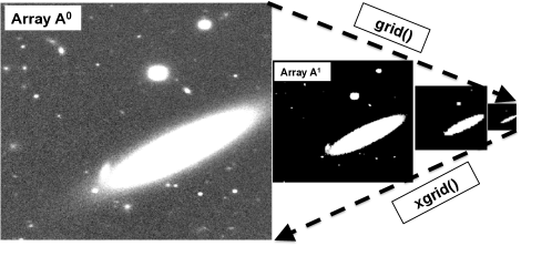
where $A^{*i}$ is the output of the iterative algorithm $Q$ on pixelated array $A^{i}$, and $A^{j-1}$ is replaced with $A_{x}^{j-1}$ as the new input for the iterative computation at pixelated version $(j-1)$.

By carefully merging the approximate results with the input array at the next finer-grained level, ArrayLoop skips a significant amount of computation.

The K-means clustering algorithm on points in a continuous space is another example application that benefits from this optimization. The KMeans application can use an arbitrary grid size. It also uses count as the aggregate function with a filter predicate that passes grid blocks that have at least one non-empty cell. It is easy to observe that in case of K-means clustering, $A_{x}^{j-1}$ is a valid labeling for the next pixelated array $A^{j-1}$. Basically, K-means clustering on $A^{j}$ produces a set of centroids for the k-means algorithm on $A^{j-1}$ that lead to a faster convergence than a random set of initial centroids.

The advantage of applying the multi-resolution optimization goes beyond better query runtime performance. This optimization can also help when the original iterative array changes, which is described as the following additional optimization:

Input Change Optimization

If ArrayLoop materializes the outputs $A^{*i}$ for all the pixelated versions of the original array $A$, then there is an interesting optimization in case the original iterative array $A$ is modified. Unlike the Naiad system [20] that materializes the entire state at each iteration to skip some computation in case of change in the input data, ArrayLoop takes a different strategy. When changes in the input occur, ArrayLoop re-generates the pixelated arrays $A^{i}$s in Equation 7, but only runs the iterative algorithm $Q$ for those arrays $A^{i}$s that have also changed in response to the input array change. If $A^{i}$ did not change for some $i$, ArrayLoop skips the computation $A^{k}\xrightarrow{Q}A^{*k}\;\forall k\geq i$ and uses the materialized result $A^{*i}$ from the previous run to produce $A_{x}^{i-1}$. The intuition is that, if there are only a few changes in the input array, it is likely that changes are not carried over to all the pixelated versions of the array and our system reuses some results of the previous run for the current computation as well.

8 Evaluation

In this section, we demonstrate the effectiveness of ArrayLoop’s native iterative processing capabilities including the three optimizations on experiments with 1TB of LSST images [24]. Because the LSST will only start to produce data in 2019, astronomers are testing their analysis pipelines with synthetic images that simulate as realistically as possible what the survey will produce. We use one such synthetic dataset. The images take the form of one large 3D array (2D images accumulated over time) with almost 44 billion non-empty cells. The experiments are executed on a 20-machine cluster. (Intel(R) Xeon(R) CPU E5-2430L @ 2.00GHz) with 64GB of memory and Ubuntu 13.04 as the operating system. We report performance for two real-scientific applications SigmaClip and SourceDetect described in Sections 2.1 and 2.2, respectively. SigmaClip runs on the large 3D array and SourceDetect runs on the co-added 2D version of the whole dataset.

8.1 Incremental Iterative Processing

We first demonstrate the effectiveness of our approach to bringing incremental processing to the iterative array model in the context of the SigmaClip application. Figure 10(a) shows the total runtime of the algorithm with different execution strategies. As shown, the non-incremental “sigma-clipping" algorithm performs almost four times worse than any other approach. The manual-incr approach is the incr-sigma-clipping function from Section 5, which is the manually-written incremental version of the “sigma-clipping" algorithm. This approach keeps track of all the points that are still candidates to be removed at the next iteration and discards the rest. By doing so, it touches the minimum number of cells from the input dataset at each iteration. Although manual-incr performs better than other approaches at later stages of the iterative computation, it incurs significant overhead during the first few iterations due to the extra data points tracking (Lines 26 to 29 in incr-sigma-clipping() function). manual-incr also requires a post-processing phase at the end of the iterative computation to return the final result. efficient-incr and efficient-incr+storage are the two strategies used by ArrayLoop (ArrayLoop-incr-sigma-clipping function from Section 5). efficient-incr represents ArrayLoop’s query rewrite for incremental state management that also leverages our merge operator. efficient-incr+storage further includes the storage manager extensions. Figure 1(a) shows the total runtime in each case. ArrayLoop’s efficient versions of the algorithm are competitive with the manually written variant. They even outperform the manual version in this application. All the incremental approaches beat the non-incremental one by a factor of $4-6X$. Interestingly, our approach to push some incremental computations to the storage manager improves efficient-incr by an extra $25\%$.

(a) SigmaClip application with different strategies.

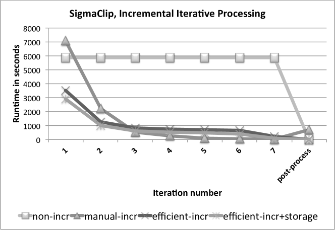
non-incr	manual-incr	efficient-incr	efficient-incr+storage
40957	10975	8007	6096

(a) Total runtime for SigmaClip for different strategies in seconds.

Figure 10: Runtime of the SigmaClip application with and without incremental processing. Constant $k=3$ in all the algorithms.

8.2 Overlap Iterative Processing

In Section 6, we describe overlap processing as a technique to support parallel array processing. In the case of an iterative computation, the challenge is to keep the overlap data up-to-date as the iteration progresses. The solution is to efficiently shuffle overlap data at each iteration. An optimization applicable to many applications is to perform mini-iteration processing, where the shuffling happens only periodically. Figure 11(a) shows the effectiveness of this optimization in the context of the SourceDetect application, which requires overlap processing. T1 refers to the policy where ArrayLoop shuffles overlap data at each iteration, or no mini-Iteration processing. As expected this approach incurs considerable data shuffling overhead, although it converges faster in the SourceDetect application (Figure 1(b)). At the other extreme, we configure ArrayLoop to only shuffle overlap data after local convergence occurs in all the chunks. Interestingly, this approach performs worse than $T1$. Although this approach does a minimum number of data shuffling, it suffers from the long tail of mini-iterations (Figure 1(b): 94 mini-iterations). $T5$ and $T10$ are two other approaches, where ArrayLoop shuffles data with some constant interval. We find that $T10$, which shuffles data every ten iterations, is a good choice in this application. The optimal interval is likely to be application-specific and tuning that value automatically is beyond the scope of this paper. The other interesting approach is to instruct ArrayLoop to initiate overlap data shuffling when the number (or magnitude) of changes between mini-iterations is below some threshold. We simply pick a constant number to determine the overlap data shuffling interval in the context of the SourceDetect application. More sophisticated approaches are left for future study.

(a) SourceDetect application: T1, T5, and T10 refer to policies where ArrayLoop shuffles overlap data every iteration, every 5 iterations, and every 10 iterations, respectively. converge is the strategy where ArrayLoop shuffles data only after local convergence occurs.

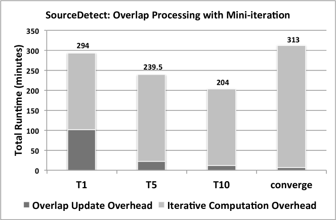
	T1	T5	T10	converge
Mini#	51	57	60	94
Major#	51	11	6	3

(b) Number of major and mini iterations. Major# is the number of times that overlap data is reshuffled and Mini# is the total number of iterations.

Figure 11: SourceDetect application: Iterative overlap processing with mini-iteration optimization.

8.3 Multi-Resolution Optimization

The multi-resolution optimization is a form of prioritized processing. By first processing a low-resolution approximation of the data, we focus on identifying the overall shape of the structures. Further processing of higher-resolution (larger) arrays then extracts the more detailed outlines of these structures. Figure 12(a) shows the benefits of this approach in the context of the SourceDetect application. We generate four lower-resolution versions of the source array A0 by sequentially calling the grid() operator with a grid-size of (2$\times$2). We operate on these multi-resolution versions exactly as described in Equation 7. The performance results are compared to those of T10 from Figure 11(a) as we pick the same overlap-processing policy to operate on each multi-resolution array. Interestingly, the multi-resolution optimization cuts runtimes nearly in half. Note that most of the saving comes from the fact that the algorithm converges much faster in $A0$ compared to its counterpart $T10$ (Figure 1(c)) thanks to the previous runs over arrays $A1$ through $A4$, where most of the cell-points are already labeled with their final cluster values.

In Section 7, we described a potential optimization in case of input data changes in the original array. As an initial evaluation of the potential of this approach, we modify the input data by dropping one image from the large, 3D array. This change is consistent with the LSST use-case, where a new set of images will be appended to the array every night. We observe that the new co-added image only differs in a small number of points from the original one. Additionally, these changes do not affect the pixelated array A1. This gives us the opportunity to re-compute the SourceDetect application not from the beginning, but from the pixelated version A1. Although the performance gain is not major in this scenario, it demonstrates the opportunity for further novel optimizations that we leave for future work.

(a) SourceDetect application: T10 refers to the strategy where ArrayLoop shuffles overlap data every 10 iterations. A0, A1, A2, A3, and A4 are five versions of the same array with different resolutions, where A0 is the same resolution as the original array and A4 is the most pixelated version. The grid-size is (2$\times$2).

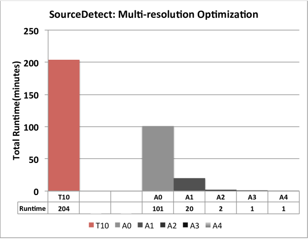
	T10	A0	A1	A2	A3	A4
iter#	60	35	12	12	6	10

(c) Iteration# that converges at each resolution.

Figure 12: SourceDetect application: Multi-resolution Optimization.

9 Related Work

Several systems have been developed that support iterative big data analytics [3, 8, 16, 29, 35]. Some have explicit iterations, others require an external driver to support iterations, but none of them provides native support for iterative computation in the context of parallel array processing.

Twister [5], Daytona [1], and HaLoop [3] extend MapReduce to add a looping construct and preserve state across iterations. HaLoop takes advantage of the task scheduler to increase local access to the static data. However, our system takes advantage of iterative array processing to increase local access to the dynamic data as well by applying overlap iterative processing.

PrIter [35] is a distributed framework for fast iterative computation. The key idea of PrIter is to prioritize iterations that ensure fast convergence. In particular, PrIter gives each data point a priority value to indicate the importance of the update and it enables selecting a subset of data rather than all the data to perform updates in each iteration. ArrayLoop also supports a form of prioritized processing through multi-resolution optimization. ArrayLoop initially finds course-grained outlines of the structures on the more pixelated versions of the array, and then it refines the details on fine-grained versions.

REX [21] is a parallel shared-nothing query processing platform implemented in Java with a focus on supporting incremental iterative computations in which changes, in the form of deltas, are propagated from iteration to iteration. Similar to REX, ArrayLoop supports incremental iterative processing. However REX lacks other optimization techniques that we provide.

A handful of systems exist that support iterative computation with focus on graph algorithms. Pregel [19] is a bulk synchronous message passing abstraction where vertices hold states and communicate with neighboring vertices. Unlike Pregel, ArrayLoop relieves the synchronization barrier overhead by including mini-iteration steps in the iterative query plan. Unlike ArrayLoop, Pregel does not prioritize iterative computation.

GraphLab [16] develops a programming model for iterative machine learning computations. The GraphLab abstraction consists of three main parts: the data graph, the dynamic asynchronous computation as update functions, and the globally sync operation. Similar to our overlap iterative processing technique, GraphLab has a notion of ghost nodes. However, the granularity of computation is per node, while ArrayLoop supports overlap iterative processing per chunk. Our system also supports prioritization through the novel multi-resolution iterative processing.

Prior work also studies array processing on in-situ data [2]. While this work addresses the limitation that array data must first be loaded into an array engine before it can be analyzed, it does not provide any special support for iterative computation. SciDB and our extensions are designed for scenarios where loading times amortize over a sufficiently large amount of data analysis.

10 Conclusion

In this paper, we developed a model for iterative processing in a parallel array engine. We then presented three optimizations to improve the performance of these types of computations: incremental processing, mini-iteration overlap processing, and multi-resolution processing. Experiments with a 1TB scientific dataset show that our optimizations can cut runtimes by 4-6X for incremental processing, 31% for overlap processing with mini-iterations, and almost 2X for the multi-resolution optimization. Interestingly, the optimizations are complementary and can be applied at the same time, cutting runtimes to a small fraction of the performance without our approach.

References

- [1] R. Barga et al. Daytona: Iterative MapReduce on Windows Azure. http://research.microsoft.com/en-us/projects/daytona/default.aspx.
- [2] Blanas et. al. Parallel data analysis directly on scientific file formats. In SIGMOD, pages 385–396, 2014.
- [3] Y. Bu et al. HaLoop: Efficient iterative data processing on large clusters. PVLDB, 3(1), 2010.
- [4] Cudre-Mauroux et. al. SS-DB: A Standard Science DBMS Benchmark. http://www-conf.slac.stanford.edu/xldb10/docs/ssdb_benchmark.pdf, 2010.
- [5] J. Ekanayake et al. Twister: a runtime for iterative MapReduce. In HPDC, pages 810–818, 2010.
- [6] E.Soroush, M.Balazinska, and D.Wang. ArrayStore: A storage manager for complex parallel array processing. In SIGMOD, pages 253–264, June 2011.
- [7] Baumann et. al. The multidimensional database system RasDaMan. In SIGMOD, pages 575–577, 1998.
- [8] S. Ewen et al. Spinning fast iterative data flows. In VLDB, pages 1268–1279, 2012.
- [9] Furtado et. al. Storage of multidimensional arrays based on arbitrary tiling. In Proc. of the 15th ICDE Conf., 1999.
- [10] Gray, J. et. al. Data cube: A relational aggregation operator generalizing group-by, cross-tab, and sub-totals. dmkd, pages 29–53, 1997.
- [11] T. Hey, S. Tansley, and K. Tolle. The fourth paradigm: Data-intensive scientific discovery, 2009.
- [12] Ž. Ivezić, A.J. Connolly, J.T. Vanderplas, and A. Gray. Statistics, Data Mining and Machine Learning in Astronomy. Princeton University Press, 2014.
- [13] Y. Kwon et al. Scalable clustering algorithm for N-body simulations in a shared-nothing cluster. In SSDBM, 2010.
- [14] Kwon, Y. et. al. Skew-resistant parallel processing of feature-extracting scientific user-defined functions. In Proc. of SOCC Symp., June 2010.
- [15] Loebman et. al. Analyzing massive astrophysical datasets: Can Pig/Hadoop or a relational DBMS help? In IASDS, 2009.
- [16] Y. Low et al. Distributed GraphLab: a framework for machine learning and data mining in the cloud. In VLDB, pages 716–727, 2012.
- [17] Large Synoptic Survey Telescope. http://www.lsst.org/.
- [18] Apache mahout. http://mahout.apache.org/.
- [19] G. Malewicz et al. Pregel: a system for large-scale graph processing. In SIGMOD, 2010.
- [20] F. McSherry, D. G. Murray, R. Isaacs, and M. Isard. Differential dataflow. In CIDR., 2013.
- [21] S.R. Mihaylov et al. REX: Recursive, delta-based data-centric computation. In VLDB, 2012.
- [22] Moyers et. al. A demonstration of iterative parallel array processing in support of telescope image analysis. In Proc. of the 39th VLDB Conf., 2013.
- [23] Nieto-santisteban et. al. Cross-matching very large datasets. In NSTC NASA Conference, 2006.
- [24] UW-CAT. http://myria.cs.washington.edu/repository/uw-cat.html.
- [25] J. Rogers et al. Overview of SciDB: Large scale array storage, processing and analysis. In SIGMOD, 2010.
- [26] SciDB Guide. http://scidb.org/HTMLmanual/13.3/scidb_ug/.
- [27] Scidb-py. http://jakevdp.github.io/SciDB-py/tutorial.html.
- [28] Seamons et. al. Physical schemas for large multidimensional arrays in scientific computing applications. In Proc of 7th SSDBM, pages 218–227, 1994.
- [29] Shaw et. al. . Optimizing large-scale semi-naive Datalog evaluation in Hadoop. In In Datalog 2.0, 2012.
- [30] Sloan Digital Sky Survey III: SkyServer DR12. http://skyserver.sdss.org/dr12/en/home.aspx.
- [31] Sloan Digital Sky Survey. http://cas.sdss.org.
- [32] Soroush et. al . Time travel in a scientific array database. In Proc. of the 29th ICDE Conf., March 2013.
- [33] Taft et. al. Genbase: A complex analytics genomics benchmark. In SIGMOD, pages 177–188, 2014.
- [34] M. Zaharia et al. Spark: cluster computing with working sets. In HotCloud’10, 2010.
- [35] Y. Zhang et al. PrIter: a distributed framework for prioritized iterative computations. In VLDB, 2011.
- [36] Zhang et. al. RIOT: I/O-efficient numerical computing without SQL. In Proc. of the Fourth CIDR Conf., 2009.