Effects of large-scale non-axisymmetric perturbations in the mean-field solar dynamo.

Abstract

We explore a response of a non-linear non-axisymmetric mean-field solar dynamo model to shallow non-axisymmetric perturbations. After a relaxation period the amplitude of the non-axisymmetric field depends on the initial condition, helicity conservation, and the depth of perturbation. It is found that a perturbation which is anchored at $0.9R_{\odot}$ has a profound effect on the dynamo process, producing a transient magnetic cycle of the axisymmetric magnetic field, if it is initiated at the growing phase of the cycle. The non-symmetric with respect to the equator perturbation results in a hemispheric asymmetry of the magnetic activity. The evolution of the axisymmetric and non-axisymmetric fields depend on the turbulent magnetic Reynolds number $R_{m}$. In the range of $R_{m}=10^{4}-10^{6}$ the evolution returns to the normal course in the next cycle, in which the non-axisymmetric field is generated due to a non-linear $\alpha$-effect and magnetic buoyancy. In the stationary state the large-scale magnetic field demonstrates a phenomenon of “active longitudes” with cyclic 180^∘ “flip-flop” changes of the large-scale magnetic field orientation. The flip-flop effect is known from observations of solar and stellar magnetic cycles. However, this effect disappears in the model which includes the meridional circulation pattern determined by helioseismology. The rotation rate of the non-axisymmetric field components varies during the relaxation period, and carries important information about the dynamo process.

1 Introduction

Dynamo theories commonly assume that the magnetic activity of the Sun is approximately axisymmetric on large spatial (size of the Sun) and temporal (the period of solar cycle) scales. These models provide a quantitative self-consistent description of the 22-year solar magnetic cycles, and allow us to investigate the basic mechanisms of the solar dynamo. However, deviations from the axisymmetry are rather strong at any particular moment of observations. Intermittent patterns of magnetic fields on the solar surface are formed because the magnetic field emerges on the surface like separated magnetic patches, e.g, in the form of sunspot groups. Such phenomena make a significant contribution to the large-scale non-axisymmetric magnetic field of the Sun.

Raedler (1986) discussed dynamo generation of large-scale non-axisymmetric (NA) magnetic field on the Sun. It was found that the differential rotation suppresses generation of the NA magnetic field. Non-linear dynamo processes can maintain a weak non-axisymmetric field in expense of the axisymmetric (AS) magnetic field (see, Raedler et al. 1990; Moss 1999; Elstner & Korhonen 2005). Also it was found that the dynamo generated NA magnetic field rotates rigidly. Further theoretical developments (see, e.g., Moss et al. 1991; Bigazzi & Ruzmaikin 2004; Moss 2004; Berdyugina et al. 2006) showed that some of the properties of the non-linear non-axisymmetric mean-field dynamo can be invoked for interpretation of the origin and evolution of the so-called “active-longitudes” of solar magnetic activity. Phenomenon of the active longitudes (AL) is probably one of the most interesting manifestations of the solar non-axisymmetric magnetic field. It appears when the solar activity persists within the fixed interval of longitudes for a long period of time (see e.g., Vitinskii 1966; Bumba & Howard 1969; Vitinsky et al. 1986).

We have to mention that the question about persistence of the AL on century time scales interval remains a highly controversial issue both from the observational and theoretical points of view. For example, Berdyugina (2004), Berdyugina et al. (2006) and Zhang et al. (2011) reported about the AL which are persistent over a century long time interval. However, Pelt et al. (2010) found that the AL have the maximal lifetime of about one solar cycle. Another phenomenon which is related to the AL is the so-called “hot spots” of the solar flare activity (Bai, 1987, 2003). The reason for the different name is because in general the longitudinal position of the activity nests is different in the Northern and Southern hemispheres. Bai (2003) found that those “hot spot could persist rigidly rotating with period about 27 days up to three solar cycles. The nonlinear dynamo models predict that the energy of the non-axisymmetric modes is only about $10^{-4}$ of the energy of the axisymmetric (AS) component (Berdyugina et al., 2006). It is not clear how such a weak magnetic field can modulate the nests of the sunspots activity.

While, the standard mean-field model can not explain the origin of the NA magnetic field (Raedler, 1986), it was noted that the solar activity produces the large-scale NA modes which are well seen in the coronal hole configurations (Stix, 1977). The very recent example of such events was observed by the SDO/HMI during the last decade of May 2015. Observations at the Wilcox Solar Observatory (Duvall et al., 1979; Hoeksema, 1995) found that the strength of the NA modes of the radial magnetic field, e.g., the mode with the azimuthal number m=1, can be about 1 G during epoch of the solar maxima. The axisymmetric dipole has the same magnitude during the solar minims. It is likely that the origin of this NA field is related to decay of solar active regions. However it is unclear how the evolution of such NA field may impact the solar dynamo process. The effect of the NA field on the global dynamo has not been studied before.

In this paper we explore a non-linear response of a mean-field dynamo model to a shallow NA m=1 perturbations with the field strength of 1G. It is assumed that these perturbations result from abrupt instability-type events, which can be described by injecting NA perturbations into the system over a very short period of time. We consider a fairly complete theoretical description of the mean turbulent electro-motive force taking into account the known properties of the solar convection zone and including the anisotropic turbulent effects due to the global rotation. The model includes a nonlinear magnetic buoyancy effect, and two types of non-linearity in the $\alpha$-effect, described as “algebraic” and “dynamical” quenching (Tworkowski et al., 1998). The algebraic quenching is due to the back-reaction of the dynamo-generated magnetic field on helical turbulence. The dynamical quenching results from a magnetic helicity conservation condition (Kleeorin & Ruzmaikin, 1982). We will show that the nonlinear non-axisymmetric effects are sufficiently strong to reproduce the “flip-flop” phenomenon and explain the rotation rate of active longitudes on the Sun (Tuominen et al., 2002a; Berdyugina et al., 2006; Gyenge et al., 2012).

2 Basic equations

Evolution of the large-scale magnetic field in perfectly conductive media is described by the mean-field induction equation (Krause & Rädler, 1980; Moffatt, 1978; Parker, 1979):

$$\partial_{t}\left\langle\mathbf{B}\right\rangle=\boldsymbol{\nabla}\times\left(\mathbf{\boldsymbol{\boldsymbol{\mathcal{E}}}+}\left\langle\mathbf{U}\right\rangle\times\left\langle\mathbf{B}\right\rangle\right)$$ (1)

where $\boldsymbol{\mathcal{E}}=\left\langle\mathbf{u\times b}\right\rangle$ is the mean electromotive force; $\mathbf{u}$ and $\mathbf{b}$ are the turbulent fluctuating velocity and magnetic field respectively; and $\left\langle\mathbf{U}\right\rangle$ and $\left\langle\mathbf{B}\right\rangle$ are the mean velocity and magnetic field. Our solution of the dynamo equation will follow the outline given earlier by Moss et al. (1991) and Moss (1999). For convenience we decompose the magnetic field into the axisymmetric (AS), (hereafter $\overline{\mathbf{B}}$-field), and non-axisymmetric (NA) parts, (hereafter $\tilde{\mathbf{B}}$-field): $\left\langle\mathbf{B}\right\rangle=\overline{\mathbf{B}}+\tilde{\mathbf{B}}$. We assume that the mean flow is axisymmetric $\left\langle\mathbf{U}\right\rangle\equiv\overline{\mathbf{U}}$. Let $\hat{\boldsymbol{\phi}}=\mathbf{e_{\phi}}$ and $\hat{\mathbf{r}}=r\mathbf{e}_{r}$ be vectors in the azimuthal and radial directions respectively, then we represent the mean magnetic field vectors as follows:

$$\left\langle\mathbf{B}\right\rangle = \overline{\mathbf{B}}+\tilde{\mathbf{B}}$$ (2)

$$\mathbf{\overline{B}} = \hat{\boldsymbol{\phi}}B+\nabla\times\left(A\hat{\boldsymbol{\phi}}\right)$$ (3)

$$\tilde{\mathbf{B}} = \boldsymbol{\nabla}\times\left(\hat{\mathbf{r}}T\right)+\boldsymbol{\nabla}\times\boldsymbol{\nabla}\times\left(\hat{\mathbf{r}}S\right),$$ (4)

where $A$, $B$, $T$ and $S$ are scalar functions representing the AS and NA parts respectively. Assuming that $A$ and $B$ do not depend on longitude, Eqs(3, 4) ensure that the field $\left\langle\mathbf{B}\right\rangle$ is divergence-free. Taking the scalar product of Eq(1) with vector $\hat{\boldsymbol{\phi}}$ we get equations for the AS magnetic field components,

$$\partial_{t}B =\hat{\boldsymbol{\phi}}\cdot\boldsymbol{\nabla}\times\left(\mathbf{\boldsymbol{\boldsymbol{\mathcal{E}}}+}\mathbf{\overline{U}}\times\overline{\mathbf{B}}\right),$$ (5)

$$\partial_{t}A =\hat{\boldsymbol{\phi}}\cdot\left(\mathbf{\boldsymbol{\mathcal{E}}+}\overline{\mathbf{U}}\times\mathbf{\overline{B}}\right),$$ (6)

To get equation for $T$ we take curl of Eq(1), and then calculate the scalar product with vector $\mathbf{\hat{r}}$. Similarly, equation for $S$ is obtained by taking twice curl of Eq(1) and then the scalar product with vector $\mathbf{\hat{r}}$. The procedure is described in detail by Krause & Rädler (1980). Equations for the NA field are

$$\partial_{t}\Delta_{\Omega}T = \Delta_{\Omega}V^{(U)}+\Delta_{\Omega}V^{(\mathcal{E})},$$ (7)

$$\partial_{t}\Delta_{\Omega}S = \Delta_{\Omega}U^{(U)}+\Delta_{\Omega}U^{(\mathcal{E})},$$ (8)

where ${\displaystyle\Delta_{\Omega}=\frac{\partial}{\partial\mu}\sin^{2}\theta\frac{\partial}{\partial\mu}+\frac{1}{\sin^{2}\theta}\frac{\partial^{2}}{\partial\phi^{2}}}$, $\mu=\cos\theta$ and $\theta$ is a polar angle, and

$$\Delta_{\Omega}V^{(U)} = -\hat{\mathbf{r}}\cdot\boldsymbol{\nabla}\times\boldsymbol{\nabla}\times\left(\mathbf{\overline{U}}\times\mathbf{\tilde{\mathbf{B}}}\right),$$ (9)

$$\Delta_{\Omega}V^{(\mathcal{E})} = -\hat{\mathbf{r}}\cdot\boldsymbol{\nabla}\times\boldsymbol{\nabla}\times\boldsymbol{\boldsymbol{\mathcal{E}}},$$ (10)

$$\Delta_{\Omega}U^{(U)} = -\hat{\mathbf{r}}\cdot\boldsymbol{\nabla}\times\left(\mathbf{\overline{U}}\times\tilde{\mathbf{B}}\right),$$ (11)

$$\Delta_{\Omega}U^{(\mathcal{E})} = -\hat{\mathbf{r}}\cdot\boldsymbol{\nabla}\times\boldsymbol{\boldsymbol{\mathcal{E}}}.$$ (12)

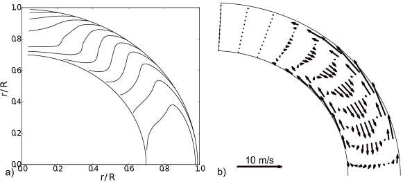
The scalar functions with superscript ^(U) contain contributions from the large-scale AS flows like the differential rotation or meridional circulation. The integration domain includes the solar convection zone from $0.71$ to $0.99R_{\odot}$. The distribution of the mean flows is given by helioseismology (Howe et al. 2011 and Zhao et al. 2013). Profiles of the angular velocity and meridional circulation are illustrated in Figure 1.

Figure 1: a) The isolines of constant angular velocity ranging from 0.6$\Omega_{0}$ to 0.96$\Omega_{0}$ ($\Omega_{0}=2.87\times 10^{-6}$s^-1); b) illustration of the double-cell meridional circulation model, consistent with the helioseismology results of Zhao et al. (2013).

We use formulation for the mean electromotive force obtained by Pipin(2008). The calculations of the mean electromotive force are done using the mean-field magnetohydrodynamics framework and the so-called “minimal tau-approximation” (see, e.g., Blackman & Field, 2002; Rädler et al., 2003; Brandenburg & Subramanian, 2005). The tau-approximation suggests that the second-order correlations do not vary significantly on timescale $\tau_{c}$ which corresponds to a typical turnover time of the convective flows. The theoretical calculations are performed for anelastic turbulent flows. They take into account the effects of density stratification, spatial inhomogeneity of the intensity of turbulent flows, and inhomogeneity of the large-scale magnetic fields. The effects of large-scale inhomogeneity of the turbulent flows and magnetic fields are computed in the first order of the Taylor expansion in terms of ratio $\ell/L$, where $\ell$ is a typical spatial scale of the turbulence, and $L$ is a spatial scale of the mean quantities. The mean electromotive force, $\boldsymbol{\mathcal{E}}$, is expressed as follows (Pipin, 2008):

$$\mathcal{E}_{i}=\left(\alpha_{ij}+\gamma_{ij}\right)\left\langle B\right\rangle_{j}-\eta_{ijk}\nabla_{j}\left\langle B\right\rangle_{k}.$$ (13)

where symmetric tensor $\alpha_{ij}$ models the generation of magnetic field by the $\alpha$- effect; antisymmetric tensor $\gamma_{ij}$ controls the mean drift of the large-scale magnetic fields in turbulent medium; tensor $\eta_{ijk}$ governs the turbulent diffusion. We take into account the effect of rotation and magnetic field on the mean-electromotive force (see, e.g., Pipin 2015 for details). To determine unique solution of Eqs.(5-8) we apply the following gauge (see, e.g., Krause & Rädler 1980; Bigazzi & Ruzmaikin 2004):

$$\int_{0}^{2\pi}\int_{-1}^{1}Sd\mu d\phi=0,\,\,\int_{0}^{2\pi}\int_{-1}^{1}Td\mu d\phi=0.$$ (14)

The same gauge is used in Eqs(9-12).

2.1 Nonlinear interaction of the axisymmetric and non-axisymmetric modes

Interaction between the AS and NA modes in the mean-field dynamo models can be due to nonlinear dynamo effects, for example, the $\alpha$-effect, (Krause & Rädler, 1980; Moss, 1999). In our model the $\alpha$ effect takes into account the kinetic and magnetic helicities in the following form:

$$\alpha_{ij} = C_{\alpha}\sin^{2}\theta\psi_{\alpha}(\beta)\alpha_{ij}^{(H)}\eta_{T}+\alpha_{ij}^{(M)}\frac{\left\langle\chi\right\rangle\tau_{c}}{4\pi\overline{\rho}\ell^{2}}$$ (15)

where $C_{\alpha}$ is a free parameter which controls the strength of the $\alpha$- effect due to turbulent kinetic helicity; $\alpha_{ij}^{(H)}$ and $\alpha_{ij}^{(M)}$ express the kinetic and magnetic helicity parts of the $\alpha$-effect, respectively; $\eta_{T}$ is the magnetic diffusion coefficient, and $\left\langle\chi\right\rangle=\left\langle\mathbf{a}\cdot\mathbf{b}\right\rangle$ ($\mathbf{a}$ and $\mathbf{b}$ are the fluctuating parts of magnetic field vector-potential and magnetic field vector). Both the $\alpha_{ij}^{(H)}$ and $\alpha_{ij}^{(M)}$ depend on the Coriolis number $\Omega^{*}=4\pi{\displaystyle\frac{\tau_{c}}{P_{rot}}}$, where $P_{rot}$ is the rotational period, $\tau_{c}$ is the convective turnover time, and $\ell$ is a typical length of the convective flows (the mixing length). A theoretical justification for the latitudinal factor, $\sin^{2}\theta$, in Eq(15) was given by Kleeorin & Rogachevskii (2003). Function $\psi_{\alpha}(\beta)$ controls the so-called “algebraic” quenching of the $\alpha$- effect where $\beta=\left|\mathbf{\left\langle B\right\rangle}\right|/\sqrt{4\pi\overline{\rho}u^{\prime 2}}$, $u^{\prime}$ is the RMS of the convective velocity. For the case of the strong magnetic field, $\beta\gg$1, $\psi_{\alpha}\sim\beta^{-2}$ . The interaction between the axisymmetric and non-axisymmetric dynamo modes via $\psi_{\alpha}(\beta)$ is because both modes contribute to parameter $\beta$. Also, for the case $\beta>$1, the latitudinal profile of the $\alpha$ effect changes. This can affect the dynamo conditions for excitation of the NA modes. Raedler et al. (1990) and Moss (1999) discussed the evolution of NA magnetic field in a simple dynamo model with such “algebraic” quenching.

The dynamical quenching is caused by the magnetic helicity conservation (see, Kleeorin & Ruzmaikin 1982). This effect was discovered by Frisch et al. (1975) and Pouquet et al. (1975). Contribution of the magnetic helicity to the $\alpha$-effect is expressed by the second term in Eq.(15). The magnetic helicity density of turbulent field, $\left\langle\chi\right\rangle=\left\langle\mathbf{a}\cdot\mathbf{b}\right\rangle$, is governed by the conservation law (Hubbard & Brandenburg, 2012; Pipin et al., 2013):

$$\frac{\partial\left\langle\chi\right\rangle^{(tot)}}{\partial t}=-\frac{\left\langle\chi\right\rangle}{R_{m}\tau_{c}}-2\eta\left\langle\mathbf{B}\right\rangle\cdot\left\langle\mathbf{J}\right\rangle-\boldsymbol{\nabla\cdot}\boldsymbol{\boldsymbol{\mathcal{F}}}^{\chi},$$ (16)

where $\left\langle\chi\right\rangle^{(tot)}=\left\langle\chi\right\rangle+\left\langle\mathbf{A}\right\rangle\cdot\left\langle\mathbf{B}\right\rangle$ is the total magnetic helicity density of the mean and turbulent fields, $\boldsymbol{\boldsymbol{\mathcal{F}}}^{\chi}=-\eta_{\chi}\boldsymbol{\nabla}\left\langle\chi\right\rangle$ is the diffusive flux of the turbulent magnetic helicity, and $R_{m}$ is the magnetic Reynolds number. The coefficient of the turbulent helicity diffusivity, $\eta_{\chi}$, is chosen ten times smaller than the isotropic part of the magnetic diffusivity (Mitra et al., 2010): $\eta_{\chi}=\frac{1}{10}\eta_{T}$. Similarly to the magnetic field, the mean magnetic helicity density can be formally decomposed into the axisymmetric and non-axisymmetric parts: $\left\langle\chi\right\rangle^{(tot)}=\overline{\chi}^{(tot)}+\tilde{\chi}^{(tot)}$. The same can be done for the magnetic helicity density of the turbulent field: $\left\langle\chi\right\rangle=\overline{\chi}+\tilde{\chi}$, where $\overline{\chi}=\overline{\mathbf{a}\cdot\mathbf{b}}$ and $\tilde{\chi}=\tilde{\left\langle\mathbf{a}\cdot\mathbf{b}\right\rangle}$. Then we have,

$$\overline{\chi}^{(tot)} =\overline{\chi}+\overline{\mathbf{A}}\cdot\overline{\mathbf{B}}+\overline{\tilde{\mathbf{A}}\cdot\tilde{\mathbf{B}}},$$ (17)

$$\tilde{\chi}^{(tot)} =\tilde{\chi}+\overline{\mathbf{A}}\cdot\tilde{\mathbf{B}}+\tilde{\mathbf{A}}\cdot\overline{\mathbf{B}}+\tilde{\mathbf{A}}\cdot\tilde{\mathbf{B}},$$ (18)

Evolution of the $\overline{\chi}$ and $\tilde{\chi}$ is governed by the corresponding parts of Eq(16). Thus, the model takes into account contributions of the AS and NA fields in the whole magnetic helicity density balance, providing a non-linear coupling. We see that the $\alpha$-effect is dynamically linked to the longitudinally averaged magnetic helicity of the NA $\tilde{\mathbf{B}}$-field, which is the last term in Eq(17). Thus, the nonlinear $\alpha$-effect is non-axisymmetric, and it results in coupling between the AS and NA modes. The coupling works in both directions. For instance, the azimuthal $\alpha$-effect results in $\mathcal{E}_{\phi}=\alpha_{\phi\phi}\left\langle B_{\phi}\right\rangle$. If we denote the NA part of the $\alpha_{\phi\phi}$ by $\tilde{\alpha}_{\phi\phi}$ then the mean electromotive force is $\overline{\mathcal{E}}_{\phi}=\overline{\alpha}_{\phi\phi}\overline{B}_{\phi}+\overline{\tilde{\alpha}_{\phi\phi}\tilde{B}_{\phi}}$. This introduces a new source in Eq(6) which is usually ignored in the axisymmetric dynamo models.

Magnetic buoyancy is another nonlinear effect which is important in the large-scale dynamo. The part of the mean electro-motive force which is responsible for magnetic buoyancy is (Kichatinov & Pipin, 1993):

$$\boldsymbol{\boldsymbol{\mathcal{E}}}^{(\beta)}=V_{\beta}\hat{\mathbf{r}}\times\mathbf{B},$$ (19)

where $V_{\beta}={\displaystyle C_{\beta}\frac{\alpha_{MLT}u^{\prime}}{\gamma}}\beta^{2}K\left(\beta\right),$ $u^{\prime}$ is the RMS convection velocity, $K\left(\beta\right)$ can be found in (Kichatinov & Pipin, 1993; Pipin, 2015), $\gamma$ is the adiabatic exponent, $\alpha_{MLT}$ is the mixing-length theory parameter, $C_{\beta}$ is a free parameter to switch on/off this effect in the model. For the case $\beta\ll 1$, $K\sim 1$ and the up-flow velocity, $V_{\beta}$, is proportional to the pressure of large-scale magnetic field. Similarly to the $\alpha$-effect, the $V_{\beta}$ is non-axisymmetric and contributes to the source terms in Eqs(5,6). Note that advection of the large-scale magnetic field by the magnetic buoyancy reduces concentration of the magnetic field near the bottom of the convection zone, and increases the field strength near the top.

2.2 Parameters of the convection zone and numerical procedure

The distribution of the turbulent parameters, such as the typical convective turn-over time, $\tau_{c}$, the mixing length, $\ell$, and the RMS convection velocity, $u^{\prime}$, are taken from the solar interior model of Stix (2002). We define the mixing-length: $\ell=\alpha_{{\rm MLT}}\left|\Lambda^{(p)}\right|^{-1}$, where $\Lambda{}^{(p)}=\boldsymbol{\nabla}\log\overline{p}\,$ is the inverse pressure scale, and the mixing-length parameter $\alpha_{{\rm MLT}}=2$. The profile of the turbulent diffusivity is taken in the form $\eta_{T}=C_{\eta}{\displaystyle\frac{u^{\prime 2}\tau_{c}}{3f_{ov}\left(r\right)}}$, where $f_{ov}(r)=1+\exp\left[50\left(r_{ov}-r\right)\right]$, $r_{ov}=0.725R_{\odot}$ controls quenching of the turbulent effects near the bottom of the convection zone, which is $r_{b}=0.715R$. Free parameter $C_{\eta}$, $\left(0<C_{\eta}<1\right)$ controls the efficiency of mixing of the large-scale magnetic field by turbulence. It is usually employed to tune the period of the dynamo cycle.

The numerical scheme employs the spherical harmonics decomposition for the non-axisymmetric part of the problem, i.e., the scalar functions T and S in Eqs(7,8) are represented in the form:

$$T\left(r,\mu,\phi,t\right) =\sum\hat{T}_{l,m}\left(r,t\right)\bar{P}_{l}^{\left|m\right|}\exp\left(im\phi\right),$$ (20)

$$S\left(r,\mu,\phi,t\right) =\sum\hat{S}_{l,m}\left(r,t\right)\bar{P}_{l}^{\left|m\right|}\exp\left(im\phi\right),$$ (21)

where $\bar{P}_{l}^{m}$ is the normalized associated Legendre function of degree $l\geq 1$ and order $m\geq 1$. The simulations which we will discuss include 600 spherical harmonics ($l_{max}=28$). Note that $\hat{S}_{l,-m}=\hat{S}_{l,m}^{*}$ and the same for $\hat{T}$. We employ the pseudo-spectral approach for integration along latitude. The second-order finite differences are used for discretization int the radial direction. The numerical integration is carried out in latitude from the pole to pole and in radius from $r_{b}=0.715R_{\odot}$ to $r_{e}=0.99R_{\odot}$. All the nonlinear terms are calculated in the real space. The transformation between the spectral spherical harmonic and the real 3D space was done using the Intel Fortran FFT library. We implement algorithms of Muciaccia et al. (1997) to speed-up the transform calculations. At the bottom of the convection zone we set up a perfectly conducting boundary condition for the axisymmetric magnetic field, and for the non-axisymmetric field we set the functions $S$ and $T$ to zero. At the top of the convection zone the poloidal field is smoothly matched to the external potential field. The boundary conditions for toroidal field allow field penetrate the surface (Moss et al. (1991), Pipin & Kosovichev (2011)):

$$\delta\frac{\eta_{T}}{r_{e}}B+\left(1-\delta\right)\mathcal{E}_{\theta} = 0,$$ (22)

$$\frac{\delta}{R}T-\left(1-\delta\right)\frac{\partial T}{\partial r} = 0$$ (23)

where parameter $\delta=0.99$.

The particular choice of parameters was discussed in our previous papers (see, e.g, Pipin & Kosovichev 2014). The free parameters are $C_{\alpha}=0.04$, $C_{\delta}=\frac{1}{3}C_{\alpha}$, $C_{\eta}=\frac{1}{15}$ and the anisotropy parameter $a=3$ (see Pipin & Kosovichev 2014). The $\alpha$-effect parameter $C_{\alpha}$ is about 30% above the dynamo generation threshold. For the chosen values of $C_{\eta}$ and $a$, the turbulent diffusion coefficient in the near-surface shear layer, at $r=0.9R_{\odot}$ is about $10^{9}$m²s^-1 which is in agreement with surface observations (see, Abramenko et al. 2011). The magnetic helicity conservation is determined by the magnetic Reynolds number $R_{m}$, for which we considered values: $10^{4}$- $10^{6}$.

To investigate the influence of meridional circulation we consider two models: M1 without meridional circulation and model M2 with the double-cell meridional circulation with a characteristic velocity 10 m/s. For the model M2 we employ the larger parameter $C_{\alpha}$ because this model has a larger critical dynamo threshold (see, Pipin & Kosovichev 2013, 2014). For this value of $C_{\alpha}$ model M2 has the same magnitude of the generated AS toroidal magnetic field inside the convection zone as the model M1. The set of parameters in the models is summarized in Table 1.

To quantify the mirror symmetry type of the toroidal magnetic field relative to the equator we introduce the parity index, $P$, as follows,

$$\overline{P} = \frac{\overline{E}_{S}-\overline{E}_{A}}{\overline{E}},$$ (24)

$$\overline{E}_{S,A} = \frac{1}{4}\int\left(B\left(r_{s},\theta\right)\pm B\left(r_{s},-\theta\right)\right)^{2}\sin\theta d\theta,$$

where “$+$” corresponds to the index “S”, and “$-$” is for “A”; $\overline{E}=\overline{E}_{S}+\overline{E}_{A}$, $\overline{E}_{S}$ and $\overline{E}_{A}$ are energies of the symmetric and anti-symmetric components of the AS toroidal magnetic field at $r_{s}=0.9R_{\odot}$ . Similarly we define parameter $\tilde{P}$ for the NA magnetic field,

$$\tilde{P} = \frac{\tilde{E}_{S}-\tilde{E}_{A}}{\tilde{E}},$$ (25)

$$\tilde{E}_{S,A} = \int\left(\tilde{B}_{\phi}\left(r_{s},\theta,\phi\right)\pm\tilde{B}_{\phi}\left(r_{s},-\theta,\phi\right)\right)^{2}\sin\theta d\theta d\phi,$$

where $\tilde{E}=\tilde{E}_{S}+\tilde{E}_{A}$. The parity of the total magnetic field is $P=\left(\overline{P}\overline{E}+\tilde{P}\tilde{E}\right)/\left(\overline{E}+\tilde{E}\right)$. We will see that perturbation can affect the cycle amplitude. Similar to Raedler et al. (1990) we introduce a parameter to measure deviation of the toroidal magnetic field from symmetry about the axis of rotation

$$M=1-\frac{\overline{E}}{\overline{E}+\tilde{E}}.$$ (26)

Figure 2: Axisymmetric and non-axisymmetric field structure at the moment of initialization of the non-axisymmetric perturbation: a) distribution of the axisymmetric toroidal magnetic field (background image) and poloidal field lines in the meridional cross-section for model M1; b) the same as a) for model M2; c) components of the non-axisymmetric magnetic field at the surface, $\tilde{B}_{r}$ is shown as color image, $\tilde{B}_{\phi}$ is shown by contour lines plotted every 3G; d) illustration of the magnetic field lines in model M1 at the moment of initialization of the perturbation.

We simulate the sunspot number $W$ using the anzatz (Pipin et al., 2012):

$$W\left(t\right)=\left\langle B_{{\rm max}}\right\rangle\exp\left(-\frac{B_{0}}{\left\langle B_{{\rm max}}\right\rangle}\right),$$ (27)

where in model M1 $\left\langle B_{{\rm max}}\right\rangle$ is the maximum strength of the toroidal magnetic field averaged in the subsurface layers over radius in the range of $0.9-0.99R_{\odot}$, and $B_{0}$ is a characteristic strength of the toroidal magnetic field, $B_{0}=800$G. In model M2 we measure $\left\langle B_{{\rm max}}\right\rangle$ in the layer of convergence of the two meridional circulation cells, which is in the range of $0.85-0.9R_{\odot}$. This layer corresponds to the maximum of the toroidal magnetic field strength in the convection zone for model M2. The AS model with the double-cell meridional circulation was discussed in details in our previous papers (Pipin & Kosovichev, 2013, 2014).

2.3 Initial conditions

In our first runs the weak initial field, which consisted of a superposition sum of polar and equatorial dipoles with the magnetic field strength of $0.01$G, evolved to a state in which the axisymmetric dynamo regime dominates. In this regime, the typical strength of the axisymmetric toroidal field in the convection zone is about 1kG. However, the non-axisymmetric field is rather weak with the strength about 10^-5G. This means that in our model the non-axisymmetric magnetic field is linearly stable, unless the dynamo governing parameters are forced to be non-axisymmetric, e.g., like in the paper by Bigazzi & Ruzmaikin (2004).

Exploring the nonlinear solutions we found that the evolution of the non-axisymmetric field depends on the initial conditions which include the strength and geometry of both the axisymmetric $\mathbf{\overline{B}}$-field and non-axisymmetric $\mathbf{\tilde{\mathbf{B}}}$-field. The evolution of the large-scale magnetic field depends on the presence of the meridional circulation, too.

In the following section we present results for the non-axisymmetric dynamo which was perturbed by a finite-amplitude non-axisymmetric $\mathbf{\tilde{\mathbf{B}}}$-field in the developed axisymmetric dynamo regime. Such non-axisymmetric perturbations can be developed either due to evolution of active regions or due to instabilities not described by the mean-field theory (e.g., Dikpati & Gilman 2001). For the seed field we consider a non-symmetric relative to the equator perturbation represented by a sum of the equatorial dipole (l=1, m=$\pm$1) and quadrupole ($l=2$, $m=\pm 1$) components. In Eq(21) we define

$$S_{1,1} =\frac{1}{2}\left(1-\mathrm{erf}\left(\frac{\left(r_{s}-r\right)}{d}\right)\right)\frac{r_{e}}{r},$$ (28)

$$S_{1,2} =\frac{1}{2}\left(1-\mathrm{erf}\left(\frac{\left(r_{s}-r\right)}{d}\right)\right)\left(\frac{r_{e}}{r}\right)^{2},$$ (29)

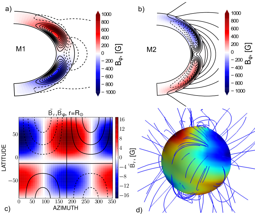
where, $r_{e}=0.99R_{\odot}$, $r_{s}=0.9R_{\odot}$ is the bottom of the subsurface shear layer, $d=0.02R_{\odot}$. The other $S_{l,m}$ and $T_{l,m}$ coefficients are zero in the perturbation. The initial non-axisymmetric perturbation is concentrated in the near-surface shear layer. The depth of the non-axisymmetric perturbation can influence the evolution of the axisymmetric dynamo. At the moment of the initialization of perturbation the strength of the axisymmetric toroidal field is by two orders of magnitude greater than of the non-axisymmetric one. At the same time the maximum amplitude of the NA radial magnetic field at the surface is about twice of the axisymmetric one (see Fig. 2c). Also, the initialization time we have the following parameters for the parity of the AS and NA parts are $\overline{P}=-1$, $\tilde{P}=-0.3$ respectively and the indexes of the axisymmetry are $M\approx 10^{-4}$.

Table 1: Summary of the dynamo models and their parameters.

Components	M1	M2
The $\boldsymbol{\mathcal{E}}$	Eq.(13)	same
circulation	no	$\overline{U}=10$m/s
free parameters, (see,Pipin 2015)	$C_{\alpha}=0.04$,$C_{\delta}=C_{\alpha}/3$, $C_{\eta}=0.06$, a=3, $C_{\beta}=1$ and $C_{\beta}=C_{\eta}$, $R_{m}=10^{4-6}$, $\alpha_{MLT}=2$	$C_{\alpha}=0.05$, others are same as in M1

3 Results

Figure 2 illustrates the geometry of the axisymmetric and non-axisymmetric fields just before initialization of the non-axisymmetric perturbation. The perturbation is initialized at $t\approx 13.2$ years for model M1 and $t\approx 5.7$ for model M2. Those times corresponds approximately the same phase of the AS toroidal magnetic field in the upper half of the convection zone in the models. Figure 3 illustrates the evolution of the axisymmetric magnetic field before and after the perturbation for two models, with and without the meridional circulation. We show the time-latitude diagrams for the toroidal magnetic field in the subsurface shear layer and the radial magnetic field at the surface. In the model with the meridional circulation the toroidal magnetic field is shown for the middle of the convection zone (see Pipin & Kosovichev 2013). The radial evolution is shown for $30^{\circ}$ latitude in the Northern hemisphere.

Figure 3: . a-c) Dynamo evolution in model M1 before and after the initialization of the non-axisymmetric perturbation at $t=13$ yr: a) time-latitude diagram, b) time-radius diagram at 30^∘ latitude, c) the simulated sunspot number for the Northern and Southern hemispheres; d-f) the same as in a-c) for model M2. Color images show the radial magnetic field component. The contour lines show the toroidal component, plotted every $100$ G.

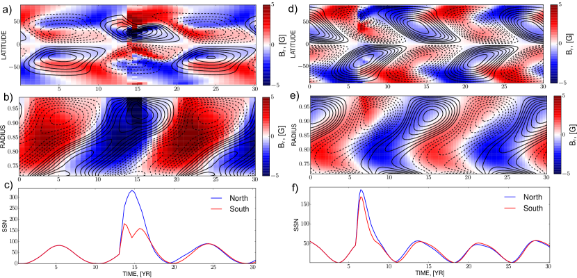
The models show that the imposed non-axisymmetric perturbation produces a transient cycle in both models M1 and in M2. In the Northern hemisphere, where the initiated perturbation is greater, the simulated sunspot number cycle is stronger than in the Southern hemisphere. The perturbation affects the reversal of the polar magnetic fields. In the Northern hemisphere the polar field reversal occurs earlier than in the Southern hemisphere where we see multiple reversals. Model M1 shows a time shift of about 2 years for the polar reversals in the Northern and Southern hemispheres. We find that these phenomena depend on the depth of perturbation (parameters, $r_{s}$ and $d$ in Eq(28)). For instance, the polar field reversal happens earlier in the Southern hemisphere than in the Northern one if the imposed perturbation is shallower $r_{s}=0.95R_{\odot}$. We also see that in both models the cycle returns quickly to the previously established axisymmetric state. Additional runs which are not illustrated here show that this restoration could take a longer time interval (more than 1 cycle) if the axisymmetric field would have a mixed parity at the initialization moment.

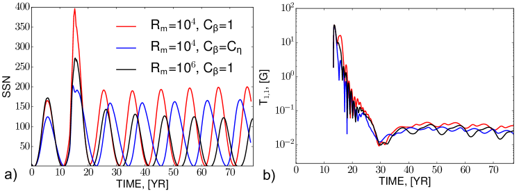
The evolution of the magnetic helicity density (Eq 16) depends on the magnetic Reynods number, $R_{m}$, which is a free parameter of the model. For higher $R_{m}$ the relaxation in both models is similar. Figure 4 illustrates the results for model M1 for $R_{m}=10^{4}$ and $R_{m}=10^{6}$ and also for model M1 with a reduced magnetic buoyancy effect ($C_{\beta}=C_{\eta}$). The developed axisymmetric dynamo regime which is employed at the beginning of evolution series shown in Figure 4 is related to the the case $R_{m}=10^{4}$ and $C_{\beta}=1$. This explains why the magnetic cycles in model M1 with $C_{\beta}=C_{\eta}$ and $R_{m}=10^{6}$ do not relax to the original cycle amplitude. The model with a reduced magnetic buoyancy shows a smaller (by a factor 2) magnitude of $T_{1,1}$ mode after the relaxation. The mode $T_{1,1}$ shows a larger variations of amplitude in case of $R_{m}=10^{6}$ than in the case of $R_{m}=10^{4}$ after the relaxation.

Figure 4: Evolution of the simulated sunspot number (a) and $T_{1,1}$ harmonic (b) in model M1 for the different values of the parameter $R_{m}$ and $C_{\beta}$: $R_{m}=10^{4}$, $C_{\beta}=1$ (red), $R_{m}=10^{4}$, $C_{\beta}=C_{\eta}$ (blue), $R_{m}=10^{6}$, $C_{\beta}=1$ (black).

Figure 5: Non-axisymmetric modes of model M1: a) the time-radius evolution of the dynamo modes $T_{1,1}$ (background image) and $S_{1,1}$ modes (contours are in the same range of values as the color scale); b) evolution of longitude of the maximum of the large-scale toroidal field, c) the mean strength of the near-surface axisymmetric and non-axisymmetric toroidal magnetic field and the strength of the m=1 T-potentials, d) evolution of parities, $\overline{P}$ and $\tilde{P}$, and the index of the axisymmetry $M$.

Figure 6: The same as Figure 5 for model M2

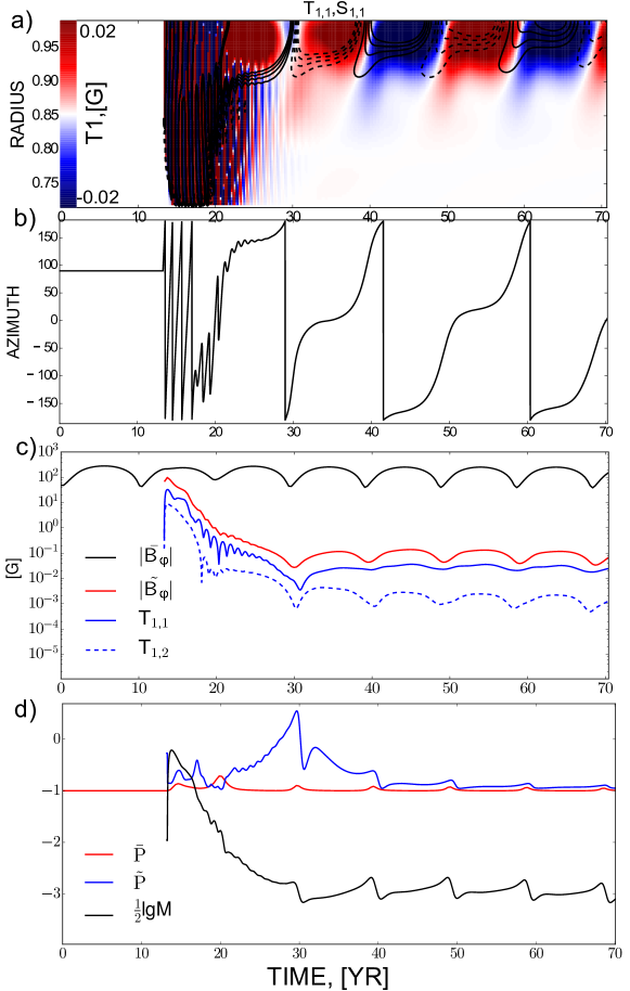
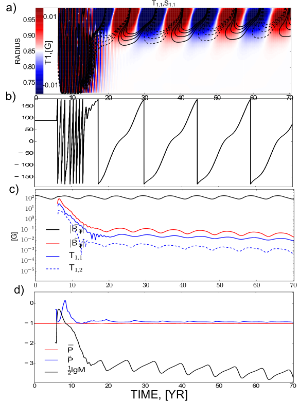
The restoration of the initial of the axisymmetric magnetic field evolution after the perturbation does not mean that the non-axisymmetric field completely dissipates. Figures 5, 6(a,c,d) show that a low strength non-axisymmetric field is maintained in the model. We find that the strength of the toroidal field T-potentials is reduced from about 100G at the maximum to 0.01G after the relaxation. In model M2 the NA magnetic field decays slowly after relaxation. Both the M1 and M2 models show a deviation of the parity of the AS magnetic field, $\overline{P}$ from -1 (corresponding to antisymmetric about theequator magnetic field) after the perturbation. The NA magnetic field shows a mixed parity solution during and after the relaxation phase. The important finding is that the NA perturbation evolves through a growing phase for about half an year in model M1 and for about one year in model M2, and it is not just decaying after the initialization. Variations of the axial symmetry index, $M$, and the parity, $P$, is shown in Fig7(a). We see that $M$ first grows and then after about 1 year the perturbation is reflected in the parity of the large-scale magnetic field. Model M1 shows greater variations of the parities than the model M2. We find that in the M1 relaxation of the parity takes more than one cycle. After relaxation the dynamo model returns to axial symmetry, $M\approx 10^{-6}$. Even such a low strength non-axisymmetric magnetic field can produce some interesting phenomena which may be related to solar observations.

Figure 7: a) Evolution of parity of total magnetic field $P$ versus the axisymmetry index $M$ for model M1 (blue) and M2(red); b) Position of maxima of the total toroidal magnetic field strength of the subsurface shear layer (r=0.92R) in models M1 and M2 after relaxation.

Figures 5,6(b) show the longitudinal evolution of a maximum of the large-scale toroidal field in the subsurface shear layer. The longitude is computed for the coordinate frame rotating with the period of about 25 days. After the perturbation initialization the longitude of the m=1 mode drifts around the Sun. There is no fluid motion associated with this drift, this drift is an analogue of the latitudinal dynamo waves in the slowly-rotating regime. The effect was suggested earlier in the study of the linear dynamo regimes by Raedler (1986). It was found in observations (e.g., Tuominen et al. 2002b; Lindborg et al. 2013) and in the direct numerical simulations (Cole et al., 2014). The speed of the drift changes after the relaxation. Model M1 shows the almost fixed positions for the longitude of the m=1 mode during epochs of the maximum of the AS toroidal magnetic field. The latitude-longitude position of the maxima of the large-scale toroidal magnetic field strength after relaxation are illustrated in Fig7(b). Model M1 (without the meridional circulation) shows the periodic changes of the longitude by 180^∘ degrees during the magnetic cycle decay. The change of the longitude is accompanied by a change of the hemispheric position of the field maximum. Thus, the orientation of the global non-axisymmetric field is reversed every cycle during the minima of the toroidal magnetic field . This behavior may correspond to the “flip-flop” phenomenon of the active longitudes suggested for stellar magnetic cycles (Berdyugina, 2004).

Model M2 which includes the meridional circulation has no stable positions of the non-axisymmetric magnetic field azimuth. Figures 5(a) and 6(a) clarify the reason for this. The effect disappears because the circulation mixes the magnetic field in the subsurface shear layer with the magnetic field of the deep interior with a period which approximately corresponds to the period of the magnetic cycle. We see that oscillations of the $S_{1,1}$ and $T_{1,1}$ harmonics have a $\pi/2$ phase shift. Thus, for a persistent appearance of the active longitude the phases of the $S_{1,1}$ and $T_{1,1}$ harmonics should be consistent. Model M2 shows a continuous drift of the longitude of the large-scale toroidal magnetic field strength in the course of the magnetic activity evolution. Additional runs which are not illustrated here show that the model with the circulation could produce a sort of active longitude phenomenon but for another combination of the circulation cells differen from the solar case shown in Figure1(b). More specifically, the strength of the bottom cell should be reduced compared to model M2. In this case we find that the active longitudes occupy only the Northern hemisphere.

Figure 8: Model M1 a half year after the initialization of the non-axisymmetric perturbation, a) distribution of the axisymmetric toroidal magnetic field (background image) and poloidal field lines in the meridional cross-section, b) azimuth-latitude distribution of the non-axisymmetric radial magnetic field (background image) and toroidal magnetic field (contours are in the same range as the color-scale) on the surface; c) the same as in panel (a) for the non-axisymmetric components of magnetic field; d) the magnetic field lines of the non-axisymmetric magnetic field above the surface.

Figure 9: The same as Figure 8 for model M2

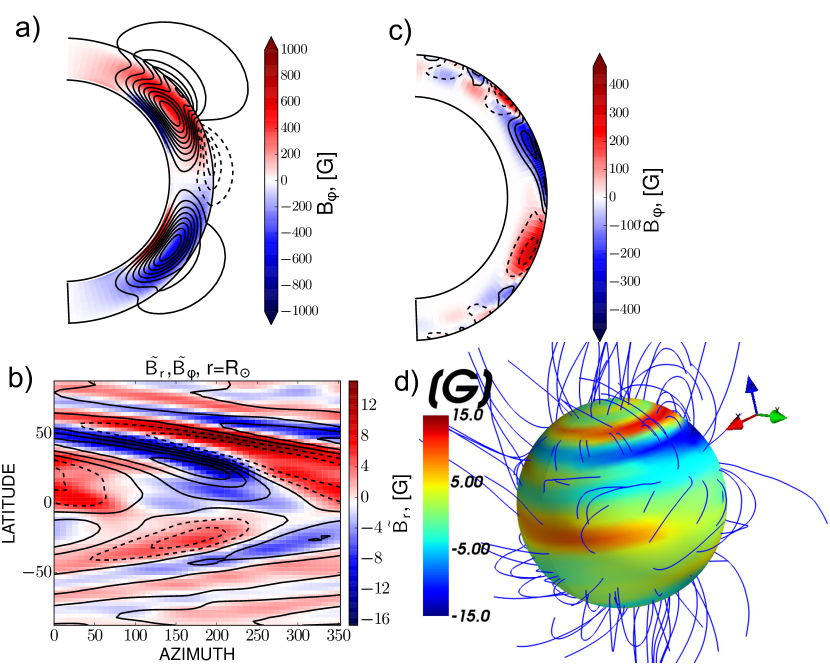
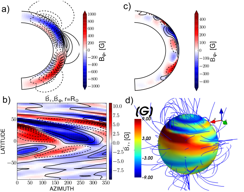
Figure 8 shows snapshots of the axisymmetric and non-axisymmetric fields after a half-year evolution of the initial perturbation. We also show the configuration of the external potential magnetic field. This period of time corresponds to a maximum of the toroidal magnetic field in the upper part of the convection zone, and the epoch of the polar field reversal. The non-axisymmetric part of the field is concentrated to the surface (as the initial field). The longitude-latitude diagram shows the distributions of the large-scale non-axisymmetric magnetic field. It illustrates how the differential rotation stretches the initial magnetic field configuration (cf., Fig2a). The snapshots in Figures 8 and 9 show the large-scale unipolar regions which extend from the equator to the high-latitude regions the poles. The increasing of the non-axisymmetric magnetic field in the polar regions results in twisted field lines in the polar caps.

Figure 10: The same as in Fig. 7 after 6 years of the evolution after the initialization of the non-axisymmetric perturbation.

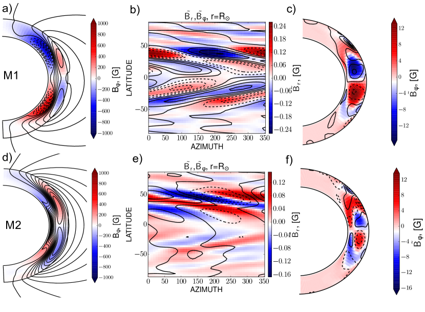
Figure 10 illustrates snapshots of the magnetic field configuration during the decaying phase of the magnetic cycle in model M1 after 6 years from the initialization. We see that the non-axisymmetric toroidal field distributed over the convection zone has maxims at the bottom of the convection zones and in the near equatorial region. The strength of the non-axisymmetric field is much smaller than the strength of the axisymmetric field. Model M2 has long overlaps between the subsequent cycles. Snapshots for this model are shown in Fig.10(bottom) for the growing phase of the cycle. The snapshots show the situation when the symmetric with respect to the equator m=1 mode dominates at the surface. In the deep layers the general distribution of the non-axisymmetric magnetic field is close to model M1.

The stationary dynamo evolution begins about 15 years after the initialization of the non-axisymmetric magnetic field in model M1 (see Fig.5). The relaxation time of model M2 is about one cycle. In the stationary stage the non-axisymmetric field is concentrated at the top of the convection zone like in the snapshots shown in Figures 8 and 9 (also see Figures 5(a) and 6(a)). The antisymmetric m=1 mode with mixed parity dominates in both models.

In addition to models M1 and M2 presented in the paper, we calculated the models for different initial conditions by changing the spatial distribution of the non-axisymmetric perturbation and the initialization time relative to the different epochs of the magnetic cycle. In model M1 the effect of perturbation is the greatest when it is initiated at the growing phase of the cycle. Also, the impact of the perturbation, and the amplitude of the non-axisymmetric field after the relaxation are stronger with the increase of the perturbation depth. However, if the perturbation in the form of Eq(28) is located near the bottom of the convection zone, it produces only a weak effect on the large-scale distributed dynamo.

Figure 11: The power spectra for rotation periods of azimuth of non-axisymmetric mode $S_{1,1}$ in the solar convection zone for: a) model M1; b) model M2.

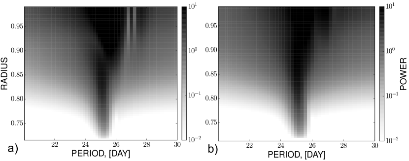
To investigate the rotation rate of the non-axisymmetric modes we calculate power spectra of the $m=1$ mode azimuth for different radii. Figure 11 shows results for the three levels of the solar convection zone. The time series cover the period of about 5 year after the initialization of the non-axisymmetric field in the models. At the initialization period the equatorial dipole was rotating with a period of 27.26 days, which corresponds to the differential rotation period at the latitude of the maxima of the initial perturbation. For model M1 it is found that in the subsurface shear layer the equatorial dipole rotates with the periods of 25.1-25.5 days. This corresponds to rotation of the subsurface shear layer at 30^∘ latitude. At the surface the dipole rotates with the period about 25.7 days, and at the bottom of the convection zone it rotates with the period of 25.1 days. The origin of these rotational periods has to be studied further. It seems that the periods of rotation follow the rotation profile in the solar convection zone, e.g., see the typical bow of the magnetic field distribution in Fig 10(c). In model M2 the meridional circulation mixes all layers of the convection zone, producing a unique maximum of the non-axisymmetric magnetic field rotating with period of 25.4 days, which corresponds to the differential rotation period at latitude of 30^∘ and $r=0.9R$.

Finally, the animated evolution of the large-scale magnetic field is illustrated by two videos: “http://www.youtube.com/watch?v=0i5tslwaxao” and
”http://www.youtube.com/watch?v=buNK91Sb3OA”, showing results for model M1.

4 Discussion and Summary

In the paper we explored the evolution of a non-axisymmetric (NA) magnetic field perturbations in the mean-field solar-type dynamo models. The models are kinematic with respect to the mean flow. The distribution of the mean flow is taken from the recent results of helioseismology, including the subsurface rotational shear layer and the double-cell meridional circulation pattern which was suggested recently by results of Zhao et al. (2013). We studied models with and without meridional circulation. The non-axisymmetric dynamo model takes into account the mean turbulent electromotive force in a fairly complete form. The mean electromotive force which is employed in the non-axisymmetric part of the model is the same as for the axisymmetric (AS) part except that the $\delta$-effect ($\Omega\times J$ term) (Rädler, 1969) was omitted in the non-axisymmetric electromotive force. We plan to investigate it separately.

The dynamo models studied in the paper show two distinct evolution phases. The transient phase starts after the initialization of the NA perturbation and ends approximately after one dynamo cycle period. The results suggest that the non-axisymmetric magnetic field can considerably affect the axisymmetric dynamo. This effect depends on the amplitude of the perturbation, the depth of perturbation, and the phase of evolution of the axisymmetric magnetic field. In the paper we illustrated the effect of a perturbation representedby the mix of the odd and even parities of $m=1$ mode of magnetic field with magnitude of 1G. The depth of the perturbation is $r=0.9R_{\odot}$ .

The models show that during the transient phase the NA magnetic field is amplified, to the level of the axysymmetry index $M=0.3$, which is 30% of the total magnetic field energy. It affects the North-South asymmetry of the magnetic field about equator. The growth and decay of the NA magnetic field is accompanied by oscillations with a period about of 1.5 year. Rotation of the$m=1$mode during the transient phase shows a continuous spectrum of the rotation periods because the evolution of the NA magnetic field is strongly coupled with the differential rotation. The maximum in the spectrum of the rotation periods is at about of 25.4 days.

The transient phase of the dynamo evolution follows by a “stationary” phase when the NA magnetic field evolves slowly, varying on the time interval which is longer than the dynamo period. Solutions for the second phase could be compared with results of the previous NA dynamo models (see, Raedler 1986; Raedler et al. 1990; Moss et al. 1991; Moss 1999; Elstner & Korhonen 2005). In the “stationary” phase we found only a weak NA magnetic field ($M\sim 10^{-6}$) with the dominant $m=1$ structure and with the antisymmetric relative to the equator magnetic parity. The NA dynamo modes rotates rigidly.

Model M1 (without the meridional circulation) shows that the rigid rotation of the m=1 dynamo modes is accompanied by changes of the longitude and the hemispheric position of the maximum of the $m=1$ mode with a period of one dynamo cycle. This regime resembles the so-called “flip-flop” phenomenon which is found in the stellar magnetic activity (Jetsu et al., 1991; Korhonen et al., 2002; Berdyugina, 2004; Lindborg et al., 2013). It was also previously suggested by other NA dynamo models (Tuominen et al., 2002b; Moss, 2004; Elstner & Korhonen, 2005; Berdyugina et al., 2006). The flip-flop phenomenon may be related another phenomenon so-called the “active longitudes” (AL) (e.g.,Vitinskii 1966; Vitinsky et al. 1986). In Introduction it was mentioned that the persistence the AL on the Sun on the century time scale remains a highly controversial issue. The origin of flip-flop phenomenon in nonlinear non-axisymmetric dynamo models was discussed in details by Moss (2004) (see, also, discussion in Berdyugina et al. 2006). In our calculations the active longitude is fixed when the $T_{1,1}$ and $S_{1,1}$ dynamo-modes are in phase. The flip-flop occurs when the orientation of the equatorial dipole changes the sign. If this effect is accompanied by the equatorial symmetry variations of the axisymmetric magnetic field then the orientation of the large-scale magnetic field changes by 180^∘. The current explanation remains qualitative because the amplitude of the NA magnetic field in the model is rather small (the axial symmetry index, $M\sim 10^{-6}$). It is not clear how such a weak NA magnetic field could modulate the sunspot activity.

One interesting feature of model M1 is that in the stationary evolution phase the antisymmetric parity of the $m=1$ mode dominates. This is different from previous results of the linear theory by Raedler (1986) and the previous nonlinear models (Raedler et al., 1990; Moss et al., 1991; Moss, 1999). Also the maximum of the $m=1$ is located on the mid-latitude zone which is different from the typical poleward concentration of the NA magnetic field suggested by results of the above cited papers. The origin of this disagreement is unclear. We have to stress that in our models we employ a fairly complete information about the radial profiles of the $\alpha$-effect and the differential rotation suggested by the modern results of the helioseismology, and results of recent theoretical works. Also we include the magnetic helicity conservation which was not taking into account before in the non-axisymmetric dynamo models. The dynamo parameters such as the $\alpha$-effect and the turbulent diffusion coefficients were tuned to reproduce the 22 year dynamo cycle by the axisymmetric dynamo. Considering the ratio between the $\alpha$ and $\Omega$-effects in our models, we find ${\displaystyle\frac{\Omega_{0}R_{\odot}}{\alpha_{0}}\sim 10^{3}}$, where $\alpha_{0}$ is the magnitude of the $\alpha$-effect. This is about by 2 orders of magnitude than the quantity employed by Raedler et al. (1990) and Moss (1999). The finding similar to ours, i.e., a concentrated to the equator antisymmetric $m=1$ magnetic field mode was reported by Nelson et al. (2013) for the global numerical simulation of the convective dynamo on the solar-type star rotating 3 times faster the modern Sun.

Model M2 with the meridional circulation illustrates another feature predicted by the linear analysis of the kinematic NA dynamo models. In this model the longitudinal position of the $m=1$ mode in the stationary phase of evolution drifts around the Sun with a period of about one dynamo cycle. This can be interpreted as an azimuthal dynamo wave. The effect was predicted by the mean-field theory (see, e.g. Krause & Rädler 1980), it was found in the mean-field NA dynamo models (Raedler, 1986; Raedler et al., 1990; Moss et al., 1991), and in the direct numerical simulations (Cole et al., 2014). It was also found in observations of magnetic activity on fast-rotating late-type stars (e.g., Tuominen et al. 2002b; Lindborg et al. 2013).

5 Conclusions

We considered non-axisymmetric mean-field dynamo models including the non-linear magnetic helicity and magnetic buoyancy effects, which were not studied before. The study confirms the previous findings of Moss (1999) that the non-axisymmetric dynamo component is rather weak if we start from a weak initial (seed) non-axisymmetric field. We notice that our models can be characterized as weakly non-linear because the parameter of the $\alpha$-effect in the model is only 30% above the dynamo instability threshold. Also the magnetic helicity conservation and magnetic buoyancy prevent the generation of magnetic field of the super-equipartition strength (Brandenburg & Käpylä, 2007; Hubbard & Brandenburg, 2012). Thus, the low-strength non-axisymmetric magnetic field generated from a weak seed field can be explained by the linear stability of the non-axisymmetric field, and by the weak non-linearity of the dynamo system. However, finite-amplitude non-axisymmetric perturbations, which can be developed in the complex dynamical system may have significant effects on the dynamo process.

The modeling results show that the magnetic helicity conservation (also known as dynamical quenching of the $\alpha$-effect) is an important factor to preserve the non-axisymmetric field from a complete decay. It is found that for the magnetic Reynolds number $R_{m}=10^{6}$ the coupling of the non-axisymmetric magnetic field with the axisymmetric dynamo process is stronger than in case of $R_{m}=10^{4}$. The strong coupling results in a synchronization between oscillations of the non-axisymmetric and axisymmetric magnetic fields. Also, our models include nonlinear effects of magnetic buoyancy. It is found that if the magnetic buoyancy effect is switched off then the strength of the non-axisymmetric field after the relaxation is decreased by a factor of two.

The paper illustrates our initial results of the nonlinear non-axisymmetric mean-field dynamo model. The axisymmetric part of the model is based on our previous results. The non-axisymmetric perturbations are assumed to be located in the near-surface rotational shear layer. For the first time we demonstrate that nonlinear coupling between the asymmetric and the non-axisymmetric fields can impact the generation of the axisymmetric field in the case of finite-amplitude perturbations. The effect depends strongly on the dynamo mechanisms involved in the problem, the spatial distribution of perturbation, the phase of the dynamo cycle at the time of initialization of the perturbation, and on how well the magnetic helicity is conserved in the system. These factors determine the subsequent evolution of the dynamo system including the dynamo cycle, evolution and rotation of the non-axisymmetric modes of large-scale magnetic fields.

In summary:

• The differential rotation and interaction with the axisymmetric magnetic fields results to amplification of the non-axisymmetric perturbation during the transient phase of evolution, producing the magnetic field configuration which deviates considerably from the axial symmetry.

• In the solar dynamo models non-axisymmetric magnetic field perturbations developed in the near-surface rotational shear layer affect the strength and period of the dynamo cycles.

• Without the meridional circulation the non-axisymmetric dynamo-mode shows a “flip-flop” phenomenon and also has a fixed longitudinal position resembling the active longitude phenomenon. However, the solar-type (double-cell) meridional circulation destroys these effects. Instead, the non-axisymmetric field represent a travelling in azimutal direction dynamo wave.

Acknowledgments The work was partially supported by NASA grants NNX09AJ85G and NNX14AB70G. VP thanks support of RFBR under grants 14-02-90424, 15-02-01407 and the project II.16.3.1 of ISTP SB RAS.

References

- Abramenko et al. (2011) Abramenko, V. I., Carbone, V., Yurchyshyn, V., Goode, P. R., Stein, R. F., Lepreti, F., Capparelli, V., & Vecchio, A. 2011, ApJ, 743, 133
- Bai (1987) Bai, T. 1987, in Bulletin of the American Astronomical Society, Vol. 19, Bulletin of the American Astronomical Society, 921
- Bai (2003) Bai, T. 2003, ApJ, 585, 1114
- Berdyugina (2004) Berdyugina, S. V. 2004, Sol. Phys., 224, 123
- Berdyugina et al. (2006) Berdyugina, S. V., Moss, D., Sokoloff, D., & Usoskin, I. G. 2006, A&A, 445, 703
- Bigazzi & Ruzmaikin (2004) Bigazzi, A., & Ruzmaikin, A. 2004, ApJ, 604, 944
- Blackman & Field (2002) Blackman, E. G., & Field, G. B. 2002, Phys. Rev. Lett., 89
- Brandenburg & Käpylä (2007) Brandenburg, A., & Käpylä, P. J. 2007, New Journal of Physics, 9, 305
- Brandenburg & Subramanian (2005) Brandenburg, A., & Subramanian, K. 2005, Phys. Rep., 417, 1
- Bumba & Howard (1969) Bumba, V., & Howard, R. 1969, Sol. Phys., 7, 28
- Cole et al. (2014) Cole, E., Käpylä, P. J., Mantere, M. J., & Brandenburg, A. 2014, ApJ, 780, L22
- Dikpati & Gilman (2001) Dikpati, M., & Gilman, P. A. 2001, ApJ, 559, 428
- Duvall et al. (1979) Duvall, Jr., T. L., Scherrer, P. H., Svalgaard, L., & Wilcox, J. M. 1979, Sol. Phys., 61, 233
- Elstner & Korhonen (2005) Elstner, D., & Korhonen, H. 2005, Astronomische Nachrichten, 326, 278
- Frisch et al. (1975) Frisch, U., Pouquet, A., Léorat, J., & A., M. 1975, J. Fluid Mech., 68, 769
- Gyenge et al. (2012) Gyenge, N., Baranyi, T., & Ludmány, A. 2012, Central European Astrophysical Bulletin, 36, 9
- Hoeksema (1995) Hoeksema, J. T. 1995, Space Sci. Rev., 72, 137
- Howe et al. (2011) Howe, R., Larson, T. P., Schou, J., Hill, F., Komm, R., Christensen-Dalsgaard, J., & Thompson, M. J. 2011, Journal of Physics Conference Series, 271, 012061
- Hubbard & Brandenburg (2012) Hubbard, A., & Brandenburg, A. 2012, ApJ, 748, 51
- Jetsu et al. (1991) Jetsu, L., Huovelin, J., Tuominen, I., & Savanov, I. 1991, A&A, 248, 574
- Kichatinov & Pipin (1993) Kichatinov, L. L., & Pipin, V. V. 1993, A&A, 274, 647
- Kleeorin & Rogachevskii (2003) Kleeorin, N., & Rogachevskii, I. 2003, Phys. Rev. E, 67, 026321
- Kleeorin & Ruzmaikin (1982) Kleeorin, N. I., & Ruzmaikin, A. A. 1982, Magnetohydrodynamics, 18, 116
- Korhonen et al. (2002) Korhonen, H., Berdyugina, S. V., & Tuominen, I. 2002, A&A, 390, 179
- Krause & Rädler (1980) Krause, F., & Rädler, K.-H. 1980, Mean-Field Magnetohydrodynamics and Dynamo Theory (Berlin: Akademie-Verlag), 271
- Lindborg et al. (2013) Lindborg, M., Mantere, M. J., Olspert, N., Pelt, J., Hackman, T., Henry, G. W., Jetsu, L., & Strassmeier, K. G. 2013, A&A, 559, A97
- Mitra et al. (2010) Mitra, D., Candelaresi, S., Chatterjee, P., Tavakol, R., & Brandenburg, A. 2010, Astronomische Nachrichten, 331, 130
- Moffatt (1978) Moffatt, H. K. 1978, Magnetic Field Generation in Electrically Conducting Fluids (Cambridge, England: Cambridge University Press)
- Moss (1999) Moss, D. 1999, MNRAS, 306, 300
- Moss (2004) —. 2004, MNRAS, 352, L17
- Moss et al. (1991) Moss, D., Tuominen, I., & Brandenburg, A. 1991, A&A, 245, 129
- Muciaccia et al. (1997) Muciaccia, P. F., Natoli, P., & Vittorio, N. 1997, ApJ, 488, L63
- Nelson et al. (2013) Nelson, N. J., Brown, B. P., Brun, A. S., Miesch, M. S., & Toomre, J. 2013, ApJ, 762, 73
- Parker (1979) Parker, E. N. 1979, Cosmical magnetic fields: Their origin and their activity (Oxford: Clarendon Press)
- Pelt et al. (2010) Pelt, J., Korpi, M. J., & Tuominen, I. 2010, A&A, 513, A48
- Pipin (2015) Pipin, V. V. 2015, MNRAS, 451, 1528
- Pipin & Kosovichev (2011) Pipin, V. V., & Kosovichev, A. G. 2011, ApJL, 727, L45
- Pipin & Kosovichev (2013) Pipin, V. V., & Kosovichev, A. G. 2013, The Astrophysical Journal, 776, 36
- Pipin & Kosovichev (2014) Pipin, V. V., & Kosovichev, A. G. 2014, ApJ, 785, 49
- Pipin et al. (2012) Pipin, V. V., Sokoloff, D. D., & Usoskin, I. G. 2012, A&A, 542, A26
- Pipin et al. (2013) Pipin, V. V., Zhang, H., Sokoloff, D. D., Kuzanyan, K. M., & Gao, Y. 2013, MNRAS, 435, 2581
- Pouquet et al. (1975) Pouquet, A., Frisch, U., & Léorat, J. 1975, J. Fluid Mech., 68, 769
- Rädler (1969) Rädler, K.-H. 1969, Monats. Dt. Akad. Wiss., 11, 194
- Rädler et al. (2003) Rädler, K.-H., Kleeorin, N., & Rogachevskii, I. 2003, Geophys. Astrophys. Fluid Dyn., 97, 249
- Raedler (1986) Raedler, K.-H. 1986, Astronomische Nachrichten, 307, 89
- Raedler et al. (1990) Raedler, K.-H., Wiedemann, E., Brandenburg, A., Meinel, R., & Tuominen, I. 1990, A&A, 239, 413
- Stix (1977) Stix, M. 1977, A&A, 59, 73
- Stix (2002) —. 2002, The sun: an introduction, 2nd edn. (Berlin : Springer), 521
- Tuominen et al. (2002a) Tuominen, I., Berdyugina, S. V., & Korpi, M. J. 2002a, Astronomische Nachrichten, 323, 367
- Tuominen et al. (2002b) —. 2002b, Astronomische Nachrichten, 323, 367
- Tworkowski et al. (1998) Tworkowski, A., Covas, E., Tavakol, R., & Brandenburg, A. 1998, ArXiv Astrophysics e-prints
- Vitinskii (1966) Vitinskii, I. I. 1966, Morfologiia solnechnoi aktivnosti.
- Vitinsky et al. (1986) Vitinsky, Y. I., Kopecky, M., & Kuklin, G. V. 1986, The statistics of sunspots (Statistika pjatnoobrazovatelnoj dejatelnosti solntsa) (Nauka, Moscow), 298pp
- Zhang et al. (2011) Zhang, L., Mursula, K., Usoskin, I., & Wang, H. 2011, A&A, 529, A23
- Zhao et al. (2013) Zhao, J., Bogart, R. S., Kosovichev, A. G., Duvall, Jr., T. L., & Hartlep, T. 2013, ApJ, 774, L29