Volumetric Bias in Segmentation and Reconstruction: Secrets and Solutions
Abstract
Many standard optimization methods for segmentation and reconstruction compute ML model estimates for appearance or geometry of segments, e.g. Zhu-Yuille [21], Torr [18], Chan-Vese [6], GrabCut [16], Delong et al. [8]. We observe that the standard likelihood term in these formulations corresponds to a generalized probabilistic K-means energy. In learning it is well known that this energy has a strong bias to clusters of equal size, which can be expressed as a penalty for KL divergence from a uniform distribution of cardinalities [10]. However, this volumetric bias has been mostly ignored in computer vision. We demonstrate significant artifacts in standard segmentation and reconstruction methods due to this bias. Moreover, we propose binary and multi-label optimization techniques that either (a) remove this bias or (b) replace it by a KL divergence term for any given target volume distribution. Our general ideas apply to many continuous or discrete energy formulations in segmentation, stereo, and other reconstruction problems.
1 Introduction
Most problems in computer vision are ill-posed and optimization of regularization functionals is critical for the area. In the last decades the community developed many practical energy functionals and efficient methods for optimizing them. This paper analyses a widely used general class of segmentation energies motivated by Bayesian analysis, discrete graphical models (e.g. MRF/CRF), information theory (e.g. MDL) , or continuous geometric formulations. Typical examples in this class of energies include a log-likelihood term for models assigned to image segments
| (1) |
where, for simplicity, we focus on a discrete formulation with data for a finite set of pixels/features and segments defined by variables/labels indicating the segment index assigned to . In different vision problems models could represent Gaussian intensity models [6], color histograms [2], GMM [21, 16], or geometric models [18, 8, 1] like lines, planes, homographies, or fundamental matrices.
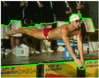
| Secrets (1) | Solutions (6), (2-10) |
 |
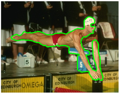 |
| (a) GrabCut [16] | with unbiased data term (10) |
 |
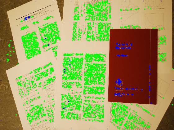 |
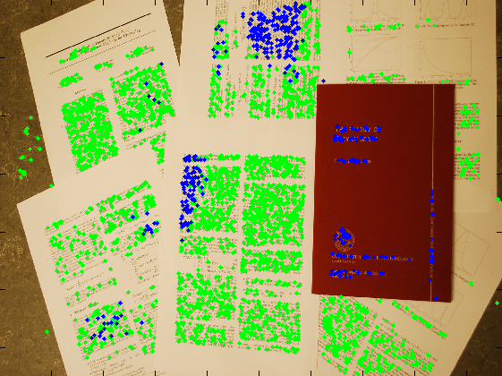
| (b) plane fitting [18, 8, 1] | with unbiased data term (10) |
 |
 |
| (c) Chan-Vese [6] [7] | with target volumes (6) |
Depending on application, the energies combine likelihoods (1), a.k.a. data term, with different regularization potentials for segments . One of the most standard regularizers is the Potts potential, as in the following energy
where is the number of label discontinuities between neighboring points on a given neighborhood graph or the length of the segmentation boundary in the image grid [3]. Another common regularizer is sparsity or label cost for each model with non-zero support [18, 21, 1, 8], e.g.
In general, energies often combine likelihoods (1) with multiple different regularizers at the same time.
This paper demonstrates practically significant bias to equal size segments in standard energies when models are treated as variables jointly estimated with segmentation . This problem comes from likelihood term (1), which we interpret as probabilistic K-means energy carefully analyzed in [10] from an information theoretic point of view. In particular, [10] decomposes energy (1) as111Symbol represents equality up to an additive constant.
where is KL divergence for model and the true distribution222The decomposition above applies to either discrete or continuous probability models (e.g. histogram vs. Gaussian). The continuous case relies on Monte-Carlo estimation of the integrals over “true” data density. of data in segment . Conditional entropy penalizes “non-deterministic” segmentation if variables are not completely determined by intensities . The last term is negative entropy of segmentation variables , which can be seen as KL divergence
| (2) |
between the volume distribution for segmentation
| (3) |
and a uniform distribution . Thus, this term represents volumetric bias to equal size segments . Its minimum is achieved for cardinalities .
1.1 Contributions
Our experiments demonstrate that volumetric bias in probabilistic K-means energy (1) leads to practically significant artifacts for problems in computer vision, where this term is widely used for model fitting in combination with different regularizers, e.g. [21, 18, 6, 16, 8]. Section 2 proposes several ways to address this bias.
First, we show how to remove the volumetric bias. This could be achieved by adding extra term to any energy with likelihoods (1) exactly compensating for the bias. We discuss several efficient optimization techniques applicable to this high-order energy term in continuous and/or discrete formulations: iterative bound optimization, exact optimization for binary discrete problems, and approximate optimization for multi-label problems using -expansion [5]. It is not too surprising that there are efficient solvers for the proposed correction term since is a concave cardinality function, which is known to be submodular for binary problems [14]. Such terms have been addressed previously, in a different context, in the vision literature [11, 17].
Second, we show that the volumetric bias to uniform distribution could be replaced by a bias to any given target distribution of cardinalities
| (4) |
In particular, introducing weights for log-likelihoods in (1) replaces bias as in (2) by divergence between segment volumes and desired target distribution
| (5) |
Our experiments in supervised or unsupervised segmentation and in stereo reconstruction demonstrate that both approaches to managing volumetric bias in (1) can significantly improve the robustness of many energy-based methods for computer vision.
2 Log-likelihood energy formulations
This section has two goals. First, we present weighted likelihood energy in (6) and show in (8) that its volumetric bias is defined by . Standard data term in (1) is a special case with . Then, we present another modification of likelihood energy in (2) and prove that it does not have volumetric bias. Note that [10] also discussed unbiased energy . The analysis of below is needed for completeness and to devise optimization for problems in vision where likelihoods are only a part of the objective function.
Weighted likelihoods: Consider energy
| (6) |
which could be motivated by a Bayesian interpretation [8] where weights explicitly come from a volumetric prior. It is easy to see that
where is a cross entropy between distributions and . As discussed in the introduction, the analysis of probabilistic K-means energy in [10] implies that
Combining two terms in the second line gives
| (8) | |||||
In case of given weights equation (8) implies that weighted likelihood term (6) has bias to the target volume distribution represented by KL divergence (5).
Note that optimization of weighted likelihood term (6) presents no extra difficulty for regularization methods in vision. Fixed weights contribute unary potentials for segmentation variables , see (2), which are trivial for standard discrete or continuous optimization methods. Nevertheless, examples in Sec. 3 show that indirect minimization of KL divergence (5) substantially improves the results in applications if (approximate) target volumes are known.
Unbiased data term: If weights are treated as unknown parameters in likelihood energy (6) they can be optimized out. In this case decomposition (8) implies that the corresponding energy has no volumetric bias:
Weights in (3) are ML estimate of that minimize (8) by achieving . Putting optimal weights into (2) confirms that volumetrically unbiased data term (2) is a combination of standard likelihoods (1) with a high-order correction term :
| (10) | |||||
Note that unbiased data term should be used with caution in applications where allowed models are highly descriptive. In particular, this applies to Zhu&Yuille [21] and GrabCut [16] where probability models are histograms or GMM. According to (2), optimization of model will over-fit to data, i.e. will be reduced to zero for arbitrary . Thus, highly descriptive models reduce to conditional entropy , which only encourages consistent labeling for points of the same color. While this could be useful in segmentation, see bin consistency in [17], trivial solution becomes good for energy . Thus, bias to equal size segments in standard likelihoods (1) is important for histogram or GMM fitting methods [21, 16].
Many techniques with unbiased data term avoid trivial solutions. Over-fitting is not a problem for simple models, e.g. Gaussians [6], lines, homographies [18, 8]. Label cost could be used to limit model complexity. Trivial solutions could also be removed by specialized regional terms added to the energy [17]. Indirectly, optimization methods that stop at a local minimum help as well.
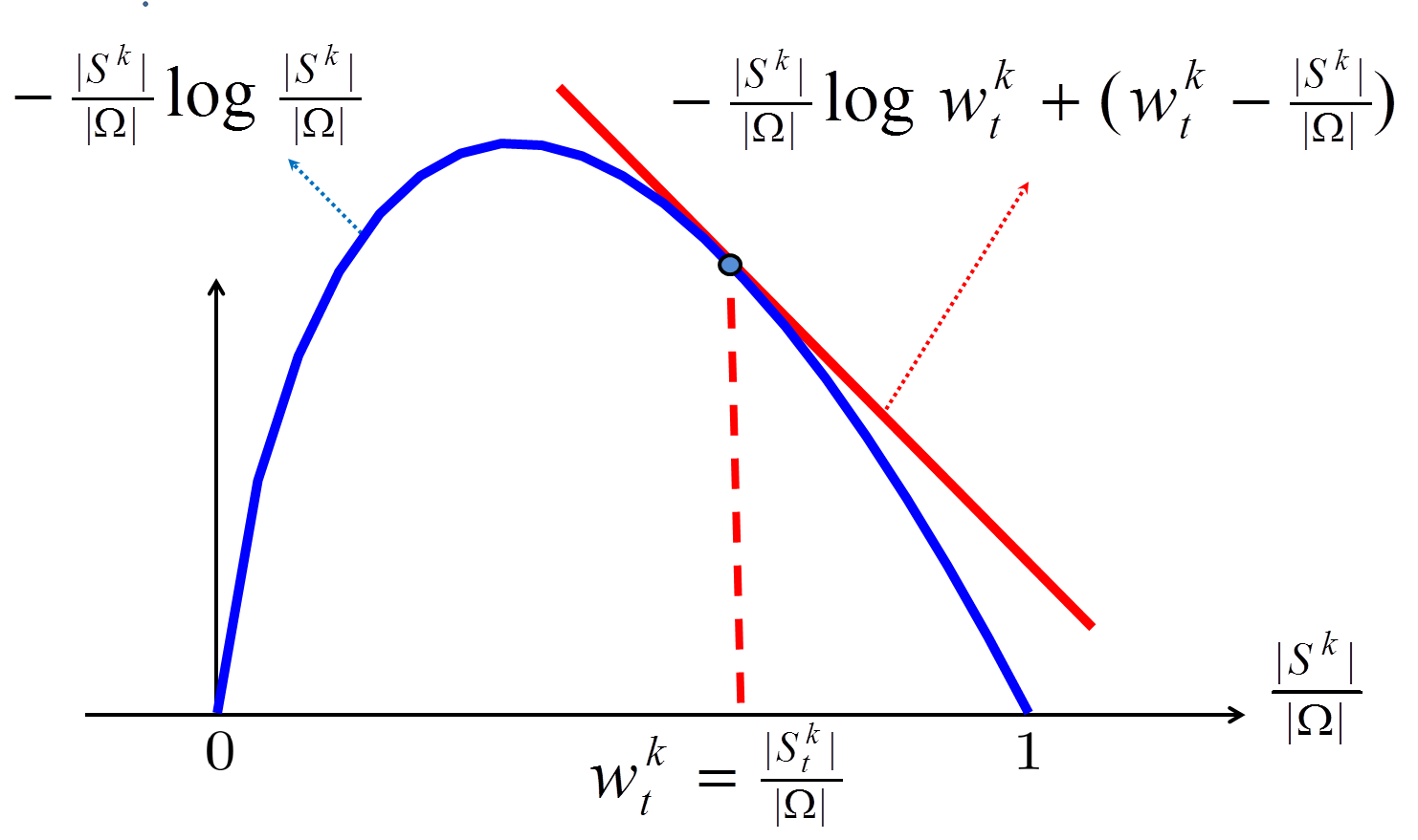
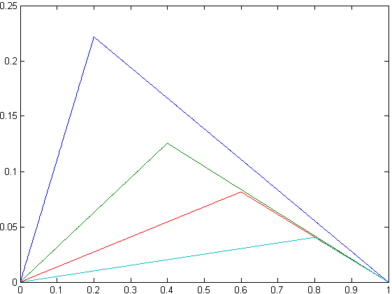
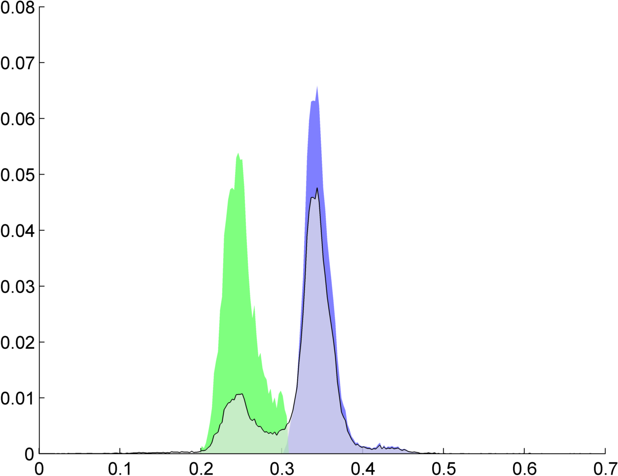
Bound optimization for (2-10): One local optimization approach for uses iterative minimization of weights for . According to (8) the optimal weights at any current solution are since they minimize . The algorithm iteratively optimizes over and resets to energy at each step until convergence. This block-coordinate descent can be seen as bound optimization [13]. Indeed, see Figure 2, at any given energy is an upper bound for , that is
This bound optimization approach to is a trivial modification for any standard optimization algorithm for energies with unary likelihood term in (6).
High-order optimization for entropy in (2-10): Alternatively, optimization of unbiased term could be based on equation (10). Since term is unary for the only issue is optimization of high-order entropy . The entropy is a combination of terms for . Each of these is a concave function of cardinality, which are known to be submodular [14]. As explained below, entropy is amenable to efficient discrete optimization techniques both in binary (Sec.3.2) and multi-label cases (Sec.3.2-3.3).
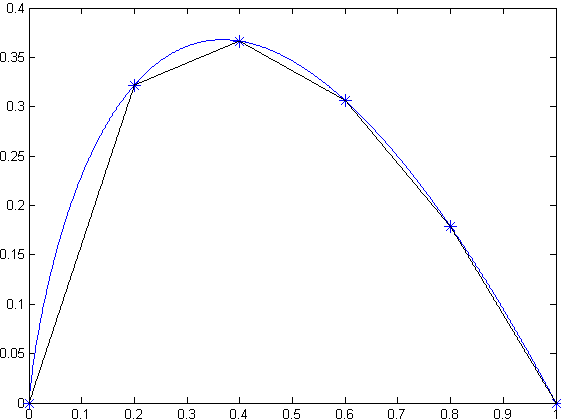
Optimization of concave cardinality functions was previously proposed in vision for label consistency [11], bin consistency [17], and other applications. Below, we discuss similar optimization methods in the context of entropy. We use a polygonal approximation with triangle functions as illustrated in Figure 3. Each triangle function is the minimum of two affine cardinality functions, yielding an approximation of the type
| (11) |
Optimization of each “triangle” term in this summation can be done as follows. Cardinality functions like and are unary. Evaluation of their minimum can be done with an auxiliary variable as in
| (12) |
which is a pairwise energy. Indeed, consider binary segmentation problems . Since
| (13) |
(12) breaks into submodular333Depending on , may need to switch and . pairwise terms for and . Thus, each “triangle” energy (12) can be globally optimized with graph cuts [12]. For more general multi-label problems energy terms (12) can be iteratively optimized via binary graph-cut moves like -expansion [5]. Indeed, let variables represent -expansion from a current solution to a new solution . Since
| (14) |
(12) also reduces to submodular pairwise terms for , .
The presented high-order optimization approach makes stronger moves than the simpler bound optimization method in the previous sub-section. However, both methods use block coordinate descent iterating optimization of and with no quality guarantees. The next section shows examples with different optimization methods.
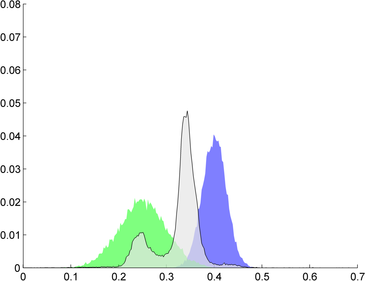
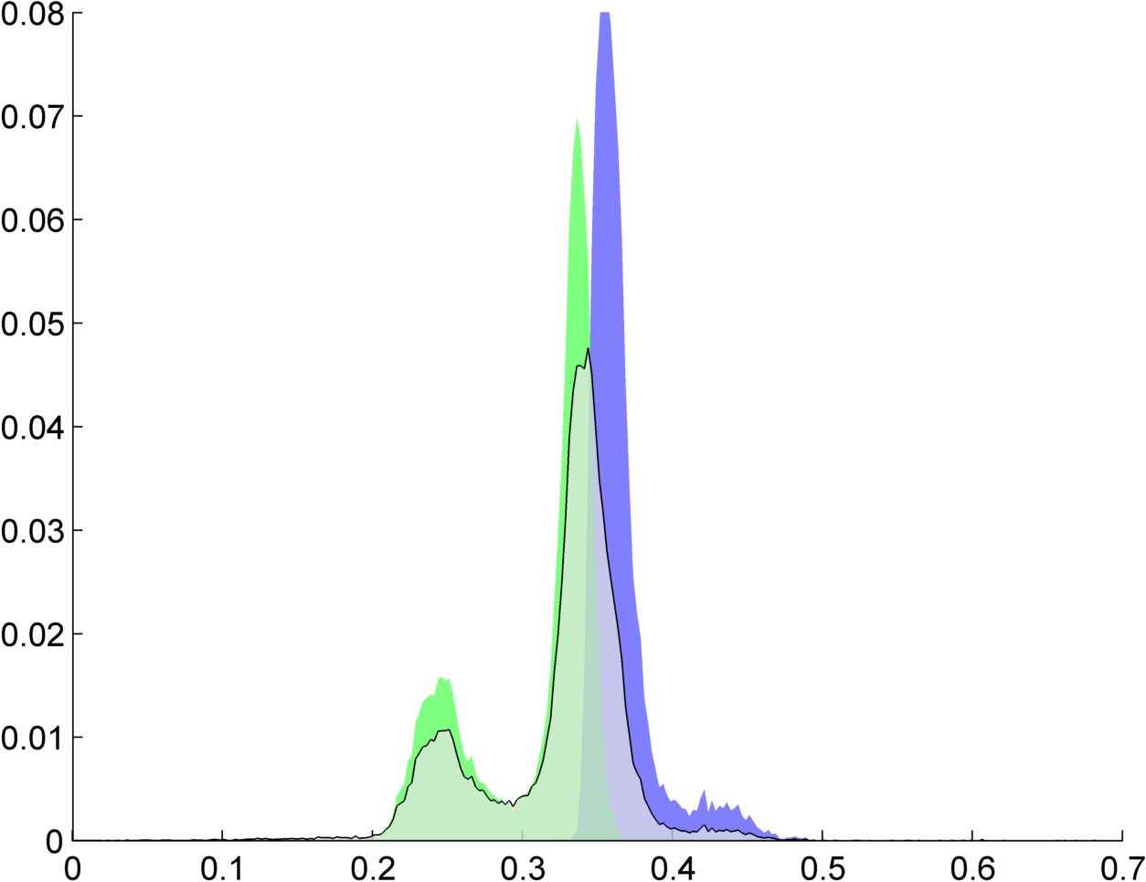
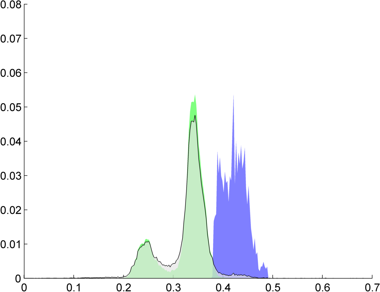
| (a) initial models | (b) segmentation for | (c) for | (d) for |
|---|---|---|---|
 |
 |
 |
 |
 |
 |
 |
 |
3 Examples
This sections considers several representative examples of computer vision problems where regularization energy uses likelihood term (1) with re-estimated models . We empirically demonstrate bias to segments of the same size (2) and show advantages of different modifications of the data term proposed in the previous section.
3.1 Segmentation with target volumes
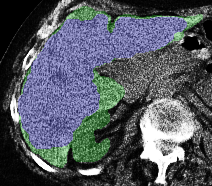
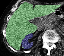
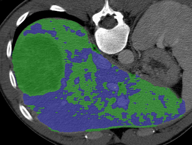
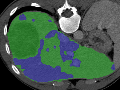
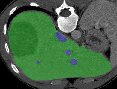
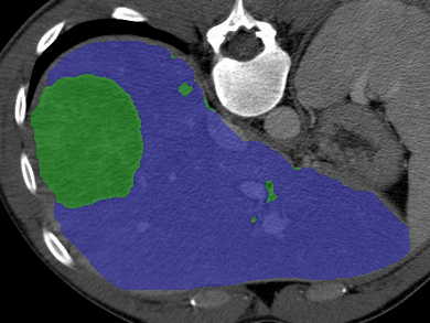
In this section we consider a biomedical example with segments: background, liver, substructure inside liver (blood vessels or cancer), see Fig.4. The energy combines standard data term from (1), boundary length , an inclusion constraint , and a penalty for distance between the background segment and a given shape template , as follows
| (15) |
For fixed models this energy can be globally minimized over as described in [7]. In this example intensity likelihood models are histograms treated as unknown parameters and estimated using block-coordinate descent for variables and . Figure 4 compares optimization of (15) in (b) with optimization of a modified energy replacing standard likelihoods with a weighted data term in (6)
| (16) |
for fixed weights set from specific target volumes (c-d).
The teaser in Figure 1(c) demonstrates a similar example for separating a kidney from a liver based on Gaussian models , as in Chan-Vese [6], instead of histograms. Standard likelihoods in (15) show equal-size bias, which is corrected by weighted likelihoods in (16) with approximate target volumes .
3.2 Segmentation without volumetric bias
We demonstrate in different applications a practically significant effect of removing the volumetric bias, i.e., using our
functional . We first report comprehensive comparisons of binary segmentations on the GrabCut data set [16], which
consists of color images with ground-truth segmentations and user-provided bounding boxes444http://research.microsoft.com/en-us/um/cambridge/projects
/visionimagevideoediting/segmentation/grabcut.htm. We compared three energies: high-order energy (10), standard likelihoods
(1), which was used in the well-known GrabCut algorithm [16], and (6), which
constrains the solution with true target volumes (i.e., those computed from ground truth). The appearance models in each energy were based on
histograms encoded by bins per channel, and the image data is based color specified in RGB coordinates. For each energy, we added a standard contrast-sensitive
regularization term [16, 2]: , where denote standard pairwise
weights determined by color contrast and spatial distance between neighboring pixels and [16, 2]. is the set neighboring
pixels in a 8-connected grid.
We further evaluated two different optimization schemes for high-order energy : (i) bound optimization and (ii) high-order optimization of concave cardinality potential using polygonal approximations; see Sec.2 for details. Each energy is optimized by alternating two iterative steps: (i) fixing the appearance histogram models and optimizing the energy w.r.t using graph cut [4]; and (ii) fixing segmentation and updating the histograms from current solution. For all methods we used the same appearance model initialization based on a user-provided box555The data set comes with two boxes enclosing the foreground segment for each image. We used the outer bounding box to restrict the image domain and the inner box to compute initial appearance models..
The error is evaluated as the percentage of mis-classified pixels with respect to the ground truth. Table 1 reports the best average error over for each method. As expected, using the true target volumes yields the lowest error. The second best performance was obtained by with high-order optimization; removing the volumetric bias substantially improves the performance of standards log-likelihoods reducing the error by . The bound optimization obtains only a small improvement as it is more likely to get stuck in weak local minima. We further show representative examples for in the last two rows of Table 1, which illustrate clearly the effect of both equal-size bias in (1) and the corrections we proposed in (10) and (6).
It is worth noting that the error we obtained for standard likelihoods (the last column in Table 1) is significantly higher than the error previously reported in the literature, e.g., [19]. The lower error in [19] is based on a different (more recent) set of tighter bounding boxes [19], where the size of the ground-truth segment is roughly half the size of the box. Therefore, the equal-size bias in (10) for this particular set of boxes has an effect similar to the effect of true target volumes in (6) (the first column in Table 1), which significantly improves the performance of standard likelihoods (the last column). In practice, both 50/50 boxes and true are equally unrealistic assumptions that require knowledge of the ground truth.
| Energy | (6) true target volumes | (10) high-order optimization | (2) bound optimization | (1) standard likelihoods |
|---|---|---|---|---|
| Overall Error (50 images) | ||||
| Examples |
![[Uncaptioned image]](/html/1505.00218/assets/Plane_Target_Volume.png) error:
error:
![[Uncaptioned image]](/html/1505.00218/assets/Bool_Target_Volume.png) error:
error:
|
![[Uncaptioned image]](/html/1505.00218/assets/Plane_High_Order.png) error:
error:
![[Uncaptioned image]](/html/1505.00218/assets/Bool_High_Order.png) error:
error:
|
![[Uncaptioned image]](/html/1505.00218/assets/Plane_Bound_Optim.png) error:
error:
![[Uncaptioned image]](/html/1505.00218/assets/Bool_Bound_Optim.png) error:
error:
|
![[Uncaptioned image]](/html/1505.00218/assets/Plane_likelihood.png) error:
error:
![[Uncaptioned image]](/html/1505.00218/assets/Bool_likelihood.png) error:
error:
|
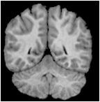
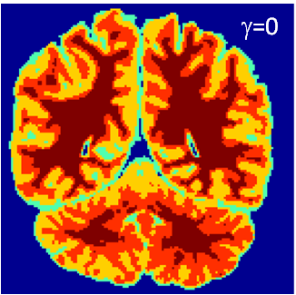
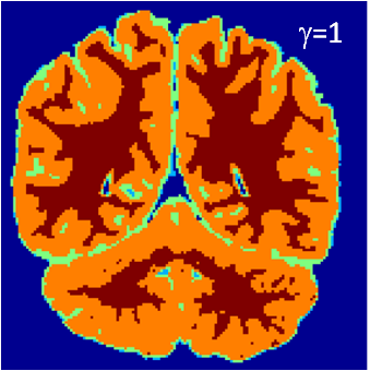
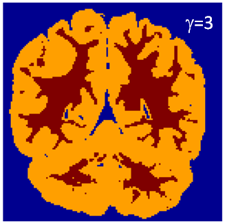
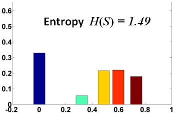
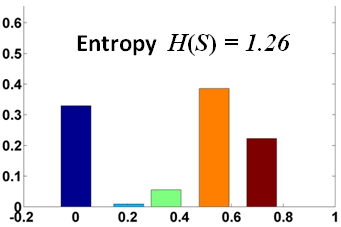
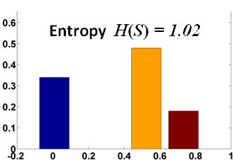
Fig. 5 depicts a different application, where we segment a magnetic resonance image (MRI) of the brain into multiple regions (). Here we introduce an extension of using a positive factor that weighs the contribution of entropy against the other terms:
| (17) |
This energy could be written as
using the high-order decomposition of likelihoods from [10] presented in the intro. Thus, the bias introduced by has two cases: (volumetric equality bias) and (volumetric disparity bias), as discussed below.
We used the Chan-Vese data term [6], which assumes the appearance models in are Gaussian distributions: , with the mean of intensities within segment and is fixed for all segments. We further added a standard total-variation term [20] that encourages boundary smoothness.
The solution is sought following the bound optimization strategy we discussed earlier; See Fig. 2. The algorithm alternates between two iterative steps: (i) optimizing a bound of w.r.t segmentation via a continuous convex-relaxation technique [20] while model parameters are fixed, and (ii) fix segmentation and update parameters and using current solution. We set the initial number of models to and fixed and . We run the method for , and . Fig. 5 displays the results using colors encoded by the region means obtained at convergence. Column (a) demonstrates the equal-size bias for ; notice that the yellow, red and brown components have approximately the same size. Setting in (b) removed this bias, yielding much larger discrepancies in size between these components. In (c) we show that using large weight in energy (17) has a sparsity effect; it reduced the number of distinct segments/labels from to . At the same time, for , this energy introduces disparity bias; notice the gap between the volumes of orange and brown segments has increased compared to in (b), where there was no volumetric bias. This disparity bias is opposite to the equality bias for in (a).
| image | equality bias | no bias | disparity bias |
 |
|
|
|
|
|
|
|
| (a) | (b) | (c) |
3.3 Geometric model fitting
Energy minimization methods for geometric model fitting problems have recently gained popularity due to [9]. Similarly to segmentation these methods are often driven by a maximum likelihood based data term measuring model fit to the particular feature. The theory presented in Section 2 applies to these problems as well and they therefore exhibit the same kind of volumetric bias.
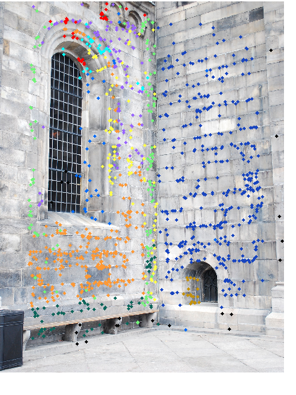
Figures 1 (b) shows a simple homography estimation example. Here we captured two images of a scene with two planes and tried to fit homographies to these (the right image with results is shown in Figure 1). For this image pair SIFT [15] generated 3376 matches on the larger plane (paper and floor) and 135 matches on the smaller plane (book). For a pair of matching points we use the log likelihood costs
| (18) |
where and is the symmetric mahalanobis transfer distance. The solution to the left in Figure 1 (b) was generated by optimizing over homographies and covariances while keeping the priors fixed and equal (). The volume bias makes the smaller plane (blue points) grab points from the larger plane. For comparison Figure 1 (b) also shows the result obtained when reestimating and . Note that the two algorithms were started with the same homographies and covariances. Figure 6 shows an independently computed 3D reconstruction using the same matches as for the homography experiment.
3.3.1 Multi Model Fitting
Recently discrete energy minimization formulations have been shown to be effective for geometric model fitting tasks [9, 8]. These methods effectively handle regularization terms needed to produce visually appealing results. The typical objective functions are of the type
| (19) |
where is a smoothness term and is a label cost preventing over fitting by penalizing the number of labels. The data term
| (20) |
consists of log-likelihoods for the observed measurements , given the model parameters . Typically the prior distributions are ignored (which is equivalent to letting all be equal) hence resulting in a bias to equal partitioning. Because of the smoothness and label cost terms the bias is not as evident in practical model fitting applications as in k-means, but as we shall see it is still present.
Multi model fitting with variable priors presents an additional challenge. The PEARL (Propose, Expand And Reestimate Labels) paradigm [9] naturally introduces and removes models during optimization. However, when reestimating priors, a model that is not in the current labeling will have giving an infinite log-likelihood penalty. Therefore a simple alternating approach (see bound optimization in Sec.2) will be unable to add new models to the solution. For sets of small cardinality it can further be seen that the entropy bound in Figure 2 will become prohibitively large since the derivative of the entropy function is unbounded (when approaching ). Instead we use -expansion moves with higher order interactions to handle the entropy term, as described in Section 2.
| (a) | (b) |
 |
 |
| (c) | (d) |
 |
 |
| (e) | (f) |
 |
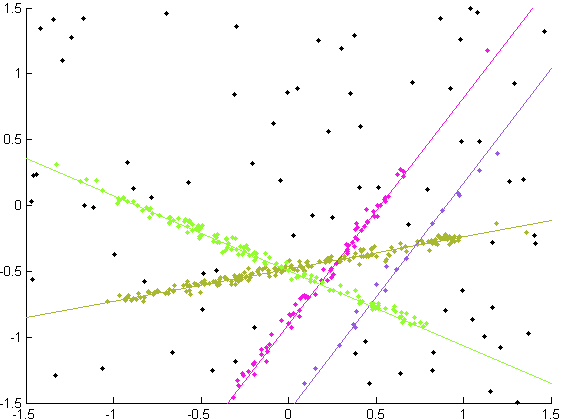 |
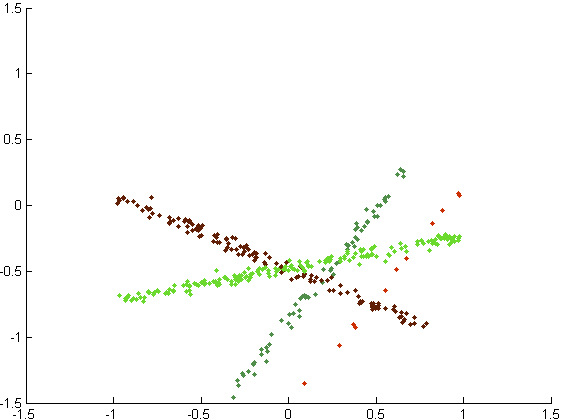
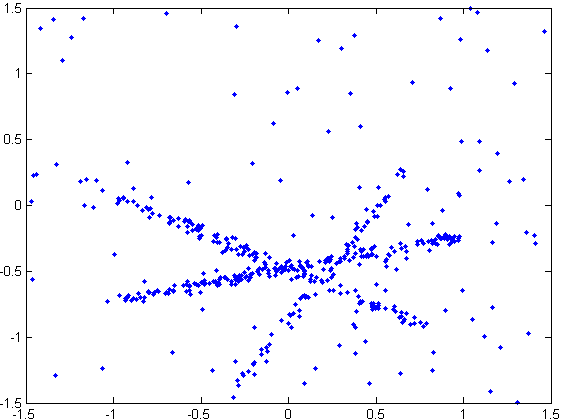
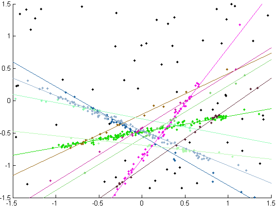
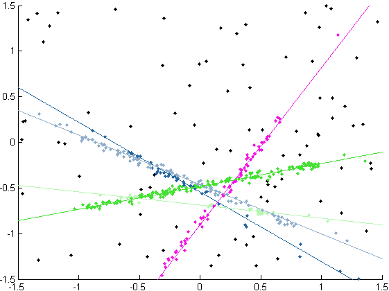
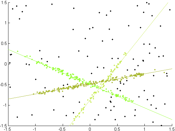
Figure 7 shows the result of a synthetic line fitting experiment. Here we randomly sampled points from four lines with different probabilities, added noise with and added outliers. We used energy (19) without smoothness and with label cost times the number of labels (excluding the outlier label). The model parameters consist of line location and orientation. We treated the noise level for each line as known. Although the volume bias seems to manifest itself more clearly when the variance is reestimated, it is also present when only the means are estimated.
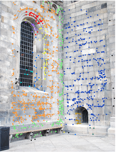
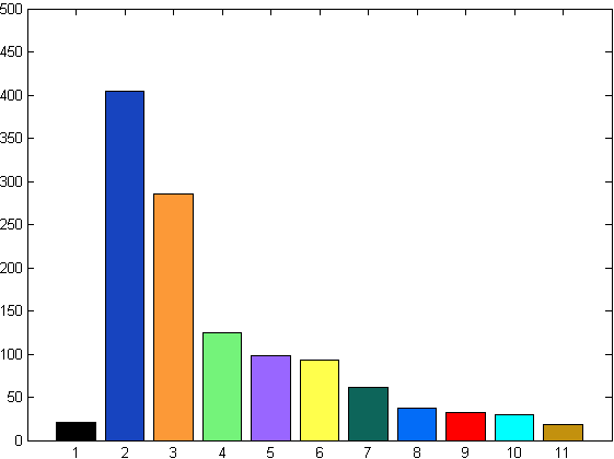
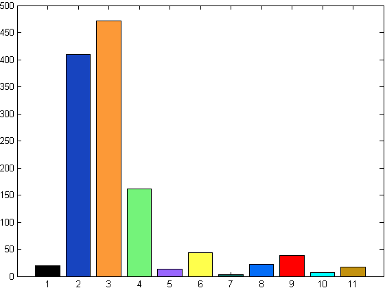
Using random sampling we generated line proposals to be used by both methods (fixed and variable W). Figure 7 (c), (d) and (e) show the results with fixed W for three different strengths of label cost. Both the label cost and the entropy term want to remove models with few assigned points. However, the label cost does not favor any assignment when it is not strong enough to remove a model. Therefore it cannot counter the volume bias of the standard data term favoring more assignments to weaker models. In the line fitting experiment of Figure 7 we varied the strength of the label cost (three settings shown in (c), (d) and (e)) without being able to correctly find all the 4 lines. Reestimation of in Figure 7 (f) resulted in a better solution.
Figures 9 and 9 show the results of a homography estimation problem with the smoothness term . For the smoothness term we followed [9] and created edges using a Delauney triangulation with weights , where is the distance between the points. For the label costs we used with fixed and with variable . We fixed the model variance to (pixels2).
4 Conclusions
We demonstrated significant artifacts in standard segmentation and reconstruction methods due to bias to equal size segments in standard likelihoods (1) following from the general information theoretic analysis [10]. We proposed binary and multi-label optimization methods that either (a) remove this bias or (b) replace it by a KL divergence term for any given target volume distribution. Our general ideas apply to many continuous or discrete problem formulations.
References
- [1] O. Barinova, V. Lempitsky, and P. Kohli. On the Detection of Multiple Object Instances using Hough Transforms. In IEEE conference on Computer Vision and Pattern Recognition (CVPR), June 2010.
- [2] Y. Boykov and M.-P. Jolly. Interactive graph cuts for optimal boundary & region segmentation of objects in N-D images. In International Conference on Computer Vision, volume I, pages 105–112, July 2001.
- [3] Y. Boykov and V. Kolmogorov. Computing geodesics and minimal surfaces via graph cuts. In International Conference on Computer Vision, volume I, pages 26–33, 2003.
- [4] Y. Boykov and V. Kolmogorov. An experimental comparison of min-cut/max-flow algorithms for energy minimization in vision. IEEE transactions on Pattern Analysis and Machine Intelligence, 26(9):1124–1137, September 2004.
- [5] Y. Boykov, O. Veksler, and R. Zabih. Fast approximate energy minimization via graph cuts. IEEE transactions on Pattern Analysis and Machine Intelligence, 23(11):1222–1239, November 2001.
- [6] T. Chan and L. Vese. Active contours without edges. IEEE Transactions on Image Processing, 10(2):266–277, 2001.
- [7] A. Delong and Y. Boykov. Globally Optimal Segmentation of Multi-Region Objects. In International Conference on Computer Vision (ICCV), 2009.
- [8] A. Delong, A. Osokin, H. Isack, and Y. Boykov. Fast Approximate Energy Minization with Label Costs. International Journal of Computer Vision (IJCV), 96(1):1–27, January 2012.
- [9] H. N. Isack and Y. Boykov. Energy-based Geometric Multi-Model Fitting. International Journal of Computer Vision (IJCV), 97(2):123–147, April 2012.
- [10] M. Kearns, Y. Mansour, and A. Ng. An Information-Theoretic Analysis of Hard and Soft Assignment Methods for Clustering. In Thirteenth Conference on Uncertainty in Artificial Intelligence (UAI), August 1997.
- [11] P. Kohli, L. Ladicky, and P. H. S. Torr. Robust Higher Order Potentials for Enforcing Label Consistency. International Journal of Computer Vision (IJCV), 82(3):302—324, 2009.
- [12] V. Kolmogorov and R. Zabih. What energy functions can be minimized via graph cuts. IEEE transactions on Pattern Analysis and Machine Intelligence, 26(2):147–159, February 2004.
- [13] K. Lange, D. R. Hunter, and I. Yang. Optimization transfer using surrogate objective functions. Journal of Computational and Graphical Statistics, 9(1):1–20, 2000.
- [14] L. Lovasz. Submodular functions and convexity. Mathematical programming: the state of the art, pages 235–257, 1983.
- [15] D. G. Lowe. Distinctive image features from scale-invariant keypoints. International Journal of Computer Vision, 60(2):91–110, 2004.
- [16] C. Rother, V. Kolmogorov, and A. Blake. Grabcut - interactive foreground extraction using iterated graph cuts. In ACM transactions on Graphics (SIGGRAPH), August 2004.
- [17] M. Tang, L. Gorelick, O. Veksler, and Y. Boykov. From GrabCut to One Cut. In International Conference on Computer Vision (ICCV), December 2013.
- [18] P. Torr. Geometric motion segmentation and model selection. Philosophical transactions of the Royal Society A, 356:1321–1340, 1998.
- [19] S. Vicente, V. Kolmogorov, and C. Rother. Joint optimization of segmentation and appearance models. In IEEE International Conference on Computer Vision (ICCV ), pages 755–762, 2009.
- [20] J. Yuan, E. Bae, X. Tai, and Y. Boykov. A continuous max-flow approach to potts model. In European Conference on Computer Vision (ECCV), Part VI, pages 379–392, 2010.
- [21] S. C. Zhu and A. Yuille. Region competition: Unifying snakes, region growing, and Bayes/MDL for multiband image segmentation. IEEE Transactions on Pattern Analysis and Machine Intelligence, 18(9):884–900, September 1996.