Non-local bias in the halo bispectrum with primordial non-Gaussianity

Matteo Tellarini    Ashley J. Ross    Gianmassimo Tasinato    and David Wands
Abstract

Primordial non-Gaussianity can lead to a scale-dependent bias in the density of collapsed halos relative to the underlying matter density. The galaxy power spectrum already provides constraints on local-type primordial non-Gaussianity complementary those from the cosmic microwave background (CMB), while the bispectrum contains additional shape information and has the potential to outperform CMB constraints in future. We develop the bias model for the halo density contrast in the presence of local-type primordial non-Gaussianity, deriving a bivariate expansion up to second order in terms of the local linear matter density contrast and the local gravitational potential in Lagrangian coordinates. Nonlinear evolution of the matter density introduces a non-local tidal term in the halo model. Furthermore, the presence of local-type non-Gaussianity in the Lagrangian frame leads to a novel non-local convective term in the Eulerian frame, that is proportional to the displacement field when going beyond the spherical collapse approximation. We use an extended Press-Schechter approach to evaluate the halo mass function and thus the halo bispectrum. We show that including these non-local terms in the halo bispectra can lead to corrections of up to 25%percent2525\% for some configurations, on large scales or at high redshift.

1 Introduction

1.1 General motivations

Inflation is a powerful mechanism to solve the puzzle of initial conditions for the Hot Big Bang cosmology and explain the origin of structure in our Universe. However, the exact mechanism that drove inflation is still a matter of debate. Different models make different predictions for the statistics of the primordial curvature perturbations ζinfsubscript𝜁inf\zeta_{\rm inf}, which can be quantified by computing the n𝑛n-point correlation functions ζinf(𝐤1)ζinf(𝐤n)delimited-⟨⟩subscript𝜁infsubscript𝐤1subscript𝜁infsubscript𝐤𝑛\langle\zeta_{\rm inf}(\mathbf{k}_{1})\dots\zeta_{\rm inf}(\mathbf{k}_{n})\rangle. All models predict some departure from Gaussianity, giving non-vanishing correlation functions for n>2𝑛2n>2. Since the amplitude, shape- and scale-dependence are model dependent, the intrinsic non-Gaussianity of primordial curvature perturbations is a powerful tool to discriminate among different models [1]. For example, local-type non Gaussianity is a distinctive signature of multi-field models [2], while equilateral and orthogonal non-Gaussianity probe non-slow roll dynamics through the self-interactions of the fields [3]. Thus observational features of the primordial curvature perturbation offer a window onto the nature of inflation [4].

At the time of this publication, the most accurate constraints on primordial non-Gaussianity (PNG) come from the cosmic microwave background (CMB). WMAP999 set the constraint on local fNLsubscript𝑓NLf_{\rm NL} to be 3<fNL<773subscript𝑓NL77-3<f_{\rm NL}<77 at 95%percent9595\% CL [5], while the most recent data from the Planck satellite experiment requires 9.2<fNL<10.89.2subscript𝑓NL10.8-9.2<f_{\rm NL}<10.8 [6]. This is compatible with the predictions of simple slowly-rolling single-field models which predict |fNL|<1subscript𝑓NL1|f_{\rm NL}|<1. The CMB is a 222D map at redshift z1100𝑧1100z\approx 1100 whose temperature fluctuations have been measured with high accuracy. The error bars could be further decreased by including the higher-resolution polarization data [7], but we are close to having fully exploited the constraining power of the CMB, being limited on small scales by the Silk damping and on large scales by the cosmic variance. The question is then which other observables may be suitable to obtain bounds on ΔfNL1Δsubscript𝑓NL1\Delta f_{\rm NL}\approx 1.

The large-scale structure (LSS) of the Universe provides a 333D map of the Universe, with accessible modes potentially going from the horizon scale 104Mpcsimilar-toabsentsuperscript104Mpc\sim 10^{4}\ \text{Mpc} down to the non-linear scale 10Mpcsimilar-toabsent10Mpc\sim 10\ \text{Mpc}. The pioneering paper by Dalal et al. [8] (see also [9]) showed that the LSS power spectrum also offers a strong constraint on primordial non-Gaussianity. The idea comes from the mode coupling in local-type models; the short wavelength modes which drive the collapse of matter into halos are modulated by the long wavelength modes, effectively changing the short-mode variance from patch to patch of the sky. This introduces a scale-dependent correction in the bias model, which describes how the number of halos relates to the matter density. Since the correction is proportional to fNL/k2subscript𝑓NLsuperscript𝑘2f_{\rm NL}/k^{2}, the clustering of structures on large scales has the potential to discriminate among different models of inflation.

It is important to emphasise that LSS constraints are independent of those from the CMB and apply on different scales, hence constraining also scale-dependent non-Gaussianity. This new perspective on the subject has been studied in depth in a number of works [9, 10, 11, 12, 13, 14, 15]. However, constraining fNLsubscript𝑓NLf_{\rm NL} from real data requires detailed understanding of the systematic errors; indeed, some of them mimic the PNG excess of power on large scales (see for instance [16, 17, 18]). Different techniques have been proposed to handle these errors [17, 19, 20, 21], as well as methods to reduce the effect of cosmic variance [22, 23, 24, 25, 26, 27] and the statistical uncertainties [28, 29]. Constraints comparable with the WMAP bounds have already been achieved [10, 30, 31, 20, 21, 32, 33, 34, 19] and even more stringent results will come thanks to the next generation of experiments, like Euclid and SKA [35, 36, 37, 27], despite the fact that no survey has been optimized for PGN so far [38]. The novel technique introduced in [39] may optimistically provide ΔfNL1similar-toΔsubscript𝑓NL1\Delta f_{\rm NL}\sim 1.

However the 222-point function is not the natural statistic in which to look for PNG, as the full shape information is available only in higher-order statistics, and moreover local-type models including higher-order non-Gaussian parameters like gNLsubscript𝑔NLg_{\rm NL} are approximately degenerate with fNLsubscript𝑓NLf_{\rm NL} in the power spectrum [40]. These issues naturally drive us towards studying higher-order n𝑛n-points correlation functions, in particular the 333-point function and its Fourier transform, the bispectrum111In [41] the possibility to use the higher-order moments of LSS to constraint PNG has been explored. Although these avoid the complexities of the full n𝑛n-point statistics, they may not be able to detect small PNG.. Many more 333D triangle configurations compared to 222D CMB ones are available in k𝑘k-space, suggesting potentially a stronger constraining power with respect to the power spectrum. Indeed, ΔfNL1Δsubscript𝑓NL1\Delta f_{\rm NL}\approx 1 is expected from the bispectrum [42, 43, 44], although this forecast is based on idealized surveys and ignores redshift space distortions (RSD). In addition, the degeneracy between fNLsubscript𝑓NLf_{\rm NL} and gNLsubscript𝑔NLg_{\rm NL} is broken by combining both the power spectrum and bispectrum constraints [45, 46].

There are a number of complications, which explains why few measurements of the 333-point function or bispectrum from real data have been obtained so far [47, 48, 42, 49, 50, 51, 52, 53, 54, 55]. For example, redshift-space distortions and the complicated mask geometry intrinsic to any survey are hard to model. Further, non-linearities in halo populations and the non-linear nature of Einstein’s field equations produce non-Gaussian features in the evolved matter field that may be hard to disentangle from the PNG signal.

1.2 What we do in this work

The ability to go beyond current constraints on PNG, crucially depends on our understanding of all possible effects that can influence LSS measurements and how these depend on the primordial fluctuations. In this paper we make improvements to the bias model which relates the halo density to the underlying matter density, particularly focussing on an accurate description of the second-order, non-local and non-Gaussian effects.

A common procedure to describe how dark matter halos trace the matter density is to assume a local relation between the final number density of objects with mass MM{\rm M} at redshift z𝑧z and the evolved density field, known as local Eulerian biasing [56],

δhE(𝐱,z,M)=j=1bjE(z)j!(δME(𝐱,z))j,superscriptsubscript𝛿E𝐱𝑧Msuperscriptsubscript𝑗1subscriptsuperscript𝑏E𝑗𝑧𝑗superscriptsubscriptsuperscript𝛿EM𝐱𝑧𝑗\delta_{h}^{\rm E}(\mathbf{x},z,{\rm M})=\sum_{j=1}^{\infty}\,\frac{b^{\rm E}_{j}(z)}{j!}\left(\delta^{\rm E}_{\rm M}(\mathbf{x},z)\right)^{j}\,, (1.1)

where bjsubscript𝑏𝑗b_{j} are the bias coefficients and δMEsubscriptsuperscript𝛿EM\delta^{\rm E}_{\rm M} is the fully non-linear density contrast in Eulerian space, smoothed on the mass scale MM{\rm M}. In this picture, the halos are drawn on top of the density field without any memory of their past history, with possible application also to the case of PNG [42, 43, 45]. However, many recent results show that this biasing model is not sufficiently accurate when compared to simulations [57, 58, 59, 60, 61]. In particular, other physically motivated contributions consistent with the symmetries of the dark matter equations of motion [62], like a tidal term, should be included. These new terms break the assumption of locality implicit in eq. 1.1. Either a local or non-local Eulerian model offer only a parametrization of the bias, and the bias coefficients need to be fitted against data or N-body simulations.

A promising alternative is to assume a physically reasonable local relation between the initial number density of objects and the initial density field [63],

δhL(𝐪,z,M)=j=1bjL(z)j!(δlin,ML(𝐪,z))j,superscriptsubscript𝛿L𝐪𝑧Msuperscriptsubscript𝑗1subscriptsuperscript𝑏L𝑗𝑧𝑗superscriptsubscriptsuperscript𝛿LlinM𝐪𝑧𝑗\delta_{h}^{\rm L}(\mathbf{q},z,{\rm M})=\sum_{j=1}^{\infty}\,\frac{b^{\rm L}_{j}(z)}{j!}\left(\delta^{\rm L}_{{\rm lin},{\rm M}}(\mathbf{q},z)\right)^{j}\,, (1.2)

where δlin,MLsubscriptsuperscript𝛿LlinM\delta^{\rm L}_{{\rm lin},{\rm M}} is the linearly evolving density contrast smoothed on scale MM{\rm M}. Note that the expansion is performed in Lagrangian space, with the initial spatial coordinate 𝐪𝐪\mathbf{q} being related to the evolved Eulerian coordinate, 𝐱𝐱\mathbf{x}, through the relation

𝐱(𝐪,τ)=𝐪+𝚿(𝐪,τ),𝐱𝐪𝜏𝐪𝚿𝐪𝜏\mathbf{x}(\mathbf{q},\tau)=\mathbf{q}+\mathbf{\Psi}(\mathbf{q},\tau)\,, (1.3)

where 𝚿𝚿\mathbf{\Psi}, the displacement field, is the key dynamical quantity in the Lagrangian picture. Equation 1.2 is known as a local Lagrangian biasing scheme and in effect assumes that the formation sites of halos can be identified from the initial density field 222Generalizations of this picture exists as well, see for instance [64, 65].. The dynamics of halos is then captured in the transformation to the Eulerian space, by applying eq. 1.3. This local Lagrangian biasing scheme comes with a prescription to calculate the bias, if we know the halo mass function, and it also automatically leads to the presence of a tidal term when written in terms of the non-linearly evolved density field [66, 57]. We will follow this approach, carefully evaluating the effects of the displacement field on the physical quantities we will investigate.

In presence of PNG of local type, the usual local Lagrangian bias model needs to be extended to account for the correlations in the initial density field. In the following we start re-deriving the bivariate model of [67], which remarkably shows good fits against simulations even when applied to the bispectrum [44, 68]. We then show that a novel non-local term arises, contributing to the number density of halos, which was previously neglected under the assumption of spherical collapse. We will quantitatively investigate how much the tidal term, and our new non-local contribution, affect the tree-level halo bispectrum in comparison with the reference model of [44] (hereafter BSS)333Alternative frameworks to include PNG of general type in a Lagrangian description exist as well. See for instance [69] and [70], which is based on the integrated perturbation theory developed in [65].


This paper is organized as follows. In section 2, we briefly introduce the main concepts and notation. In particular, in section 2.1 we review the evolution of the matter density field up to second order and indentify a new convective term in presence of PNG, while in section 2.2 we describe the peak-background split. This constitutes the basis of our local Lagrangian biasing scheme, which will be presented in section 3. As we work in a Lagrangian approach, our result then needs to be transformed into the Eulerian frame in section 4. In section 5 expressions for the matter and halo bispectra are given, and a numerical analysis of the halo bispectrum is presented in section 6, where we quantify the effect of new non-local terms in LSS bispectra. We present our final conclusions together with a discussion of potential future developments of our work in section 7.

2 Basic framework

2.1 Matter density field

In this subsection we define the quantities and introduce the notation that we will use in what follows. The linearly growing mode of the density field has a simple separable form in Lagrangian space

δlin(𝐪,z)=C(𝐪)D(z),subscript𝛿lin𝐪𝑧𝐶𝐪𝐷𝑧\delta_{\rm lin}(\mathbf{q},z)=C(\mathbf{q})D(z)\,, (2.1)

where D(z)𝐷𝑧D(z) is the linear growth factor with D(z)(1+z)1proportional-to𝐷𝑧superscript1𝑧1D(z)\propto(1+z)^{-1} in the matter-dominated era, normalized such that D(0)=1𝐷01D(0)=1.

The density contrast at the start of the matter-dominated era is determined by the primordial metric perturbation from inflation that we denote with ζinfsubscript𝜁inf\zeta_{\rm inf}. In Fourier space we have

δlin(𝐤,z)=2k2c2T(k)D(z)5ΩmH02ζinf(𝐤),subscript𝛿lin𝐤𝑧2superscript𝑘2superscript𝑐2𝑇𝑘𝐷𝑧5subscriptΩ𝑚superscriptsubscript𝐻02subscript𝜁inf𝐤\delta_{\rm lin}(\mathbf{k},z)=\frac{2k^{2}c^{2}T(k)D(z)}{5\Omega_{m}H_{0}^{2}}\,\zeta_{\rm inf}(\mathbf{k})\,, (2.2)

where the transfer function T(k)𝑇𝑘T(k) accounts for the damping of sub-Hubble-scale modes in the radiation era and T(k)1𝑇𝑘1T(k)\rightarrow 1 as k0𝑘0k\to 0. Conventionally this is written in terms of a primordial Newtonian potential

δlin(𝐤,z)=α(k,z)Φin(𝐤),subscript𝛿lin𝐤𝑧𝛼𝑘𝑧subscriptΦin𝐤\delta_{\rm lin}(\mathbf{k},z)=\alpha(k,z)\Phi_{\rm in}(\mathbf{k})\,, (2.3)

where, from eq. 2.3, we identify

Φin=35ζinf,α(k,z)2k2c2T(k)D(z)3ΩmH02.formulae-sequencesubscriptΦin35subscript𝜁inf𝛼𝑘𝑧2superscript𝑘2superscript𝑐2𝑇𝑘𝐷𝑧3subscriptΩ𝑚superscriptsubscript𝐻02\Phi_{\rm in}=\frac{3}{5}\zeta_{\rm inf}\,,\quad\alpha(k,z)\equiv\frac{2k^{2}c^{2}T(k)D(z)}{3\Omega_{m}H_{0}^{2}}\,. (2.4)

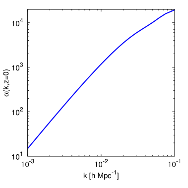
The function α𝛼\alpha is plotted in fig. 1.

Throughout this paper we will consider a primordial Newtonian potential with local-type non-Gaussianity, that is a local function of a Gaussian random field [71, 72, 73]

Φin=φG(𝐪)+fNL(φG2(𝐪)φG2),subscriptΦinsubscript𝜑G𝐪subscript𝑓NLsubscriptsuperscript𝜑2G𝐪delimited-⟨⟩subscriptsuperscript𝜑2G\Phi_{\rm in}=\varphi_{\rm G}(\mathbf{q})+f_{\rm NL}\left(\varphi^{2}_{\rm G}(\mathbf{q})-\langle\varphi^{2}_{\rm G}\rangle\right)\,, (2.5)

where φG(𝐪)subscript𝜑𝐺𝐪\varphi_{G}(\mathbf{q}) is a Gaussian field, seeded by free field fluctuations during inflation, and fNLsubscript𝑓NLf_{\rm NL} is a dimensionless parameter quantifying the magnitude of non-Gaussian corrections either due to non-linear evolution of the primordial metric perturbation [2], or to the non-linearity inherent in the general relativistic constraint equations [74, 75, 76]. Note that the non-Gaussian correction is a local function of the Gaussian field at a given initial (Lagrangian) position, 𝐪𝐪\mathbf{q}.

In the presence of primordial non-Gaussianity, the linearly growing mode (2.3) contains first- and second-order terms with respect to φG(𝐪)subscript𝜑𝐺𝐪\varphi_{G}(\mathbf{q}). It will be convenient, for our discussion, to define the first-order (Gaussian) density contrast δG(𝐤,z)subscript𝛿G𝐤𝑧\delta_{{\rm G}}(\mathbf{k},z), where from eq. 2.3 and eq. 2.5 we identify

δG(𝐤,z)=α(k,z)φG(𝐤).subscript𝛿G𝐤𝑧𝛼𝑘𝑧subscript𝜑G𝐤\delta_{{\rm G}}(\mathbf{k},z)=\alpha(k,z)\varphi_{\rm G}(\mathbf{k})\,. (2.6)
Refer to caption
(a)
Refer to caption
(b)
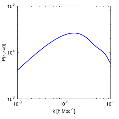
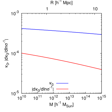
Figure 1: The left panel shows α𝛼\alpha as a function of wavenumber k𝑘k at redshift z=0𝑧0z=0. The right panel shows the matter power spectrum P(k)𝑃𝑘P(k) at redshift z=0𝑧0z=0. They are both obtained using CAMB [77] and assuming the Planck data set [78].

The initial linearly growing mode of eq. 2.3 drives the subsequent non-linear evolution of the density field [79] and we may write the non-linearly evolved field in Lagrangian coordinates as

δ𝛿\displaystyle\delta =δlin(𝐪,z)+δnonlinL(𝐪,z).absentsubscript𝛿lin𝐪𝑧superscriptsubscript𝛿nonlinL𝐪𝑧\displaystyle=\delta_{\rm lin}(\mathbf{q},z)+\delta_{\rm nonlin}^{\rm L}(\mathbf{q},z)\,. (2.7)

where at second order we have

δnonlinL(𝐪,z)subscriptsuperscript𝛿Lnonlin𝐪𝑧\displaystyle\delta^{\rm L}_{\rm nonlin}(\mathbf{q},z) 1721(δlin(𝐪,z))2+27s2(𝐪,z)similar-to-or-equalsabsent1721superscriptsubscript𝛿lin𝐪𝑧227superscript𝑠2𝐪𝑧\displaystyle\simeq\frac{17}{21}(\delta_{\rm lin}(\mathbf{q},z))^{2}+\frac{2}{7}s^{2}(\mathbf{q},z)\, (2.8)

with s2=sijsijsuperscript𝑠2subscript𝑠𝑖𝑗superscript𝑠𝑖𝑗s^{2}=s_{ij}s^{ij} and sijsubscript𝑠𝑖𝑗s_{ij}, the trace-free tidal tensor, is defined as

sij(ij13δijK)2δ,subscript𝑠𝑖𝑗subscript𝑖subscript𝑗13subscriptsuperscript𝛿𝐾𝑖𝑗superscript2𝛿s_{ij}\equiv\left(\nabla_{i}\nabla_{j}-\frac{1}{3}\delta^{K}_{ij}\right)\nabla^{-2}\delta\,, (2.9)

where δijKsubscriptsuperscript𝛿𝐾𝑖𝑗\delta^{K}_{ij} is the Kronecker delta function.

Since the Lagrangian and Eulerian coordinates (1.3) agree at leading order, the first-order density perturbation eq. 2.6 has the same form in either frame. However at second order the density perturbations differ because of the convective term proportional to the displacement, 𝚿𝚿\mathbf{\Psi} [80]444See also [81] where this term is referred to as a shift term.. For a general function f(𝐱,z)𝑓𝐱𝑧f(\mathbf{x},z) we have, from eq. 1.3,

f(𝐱(𝐪,z),z)f(𝐪,z)+𝚿f(𝐪,z).similar-to-or-equals𝑓𝐱𝐪𝑧𝑧𝑓𝐪𝑧𝚿𝑓𝐪𝑧f(\mathbf{x}(\mathbf{q},z),z)\simeq f(\mathbf{q},z)+\mathbf{\Psi}\cdot\mathbf{\nabla}f(\mathbf{q},z)\,. (2.10)

Hence we can write the non-linearly evolved density field eq. 2.7 in Eulerian coordinates as

δ𝛿\displaystyle\delta =δlin(𝐱,z)+δnonlinE(𝐱,z),absentsubscript𝛿lin𝐱𝑧superscriptsubscript𝛿nonlinE𝐱𝑧\displaystyle=\delta_{\rm lin}(\mathbf{x},z)+\delta_{\rm nonlin}^{\rm E}(\mathbf{x},z)\,, (2.11)

where at second order, using eqs. 2.8 and 2.10, we obtain [82]:

δnonlinE(𝐱,z)subscriptsuperscript𝛿Enonlin𝐱𝑧\displaystyle\delta^{\rm E}_{\rm nonlin}(\mathbf{x},z) 1721(δlin(𝐱,z))2+27s2(𝐱,z)𝚿(𝐱,z)δ(𝐱,z).similar-to-or-equalsabsent1721superscriptsubscript𝛿lin𝐱𝑧227superscript𝑠2𝐱𝑧𝚿𝐱𝑧𝛿𝐱𝑧\displaystyle\simeq\frac{17}{21}(\delta_{\rm lin}(\mathbf{x},z))^{2}+\frac{2}{7}s^{2}(\mathbf{x},z)-\mathbf{\Psi}(\mathbf{x},z)\cdot\mathbf{\nabla}\delta(\mathbf{x},z)\,. (2.12)

Similarly, although the Newtonian potential has the same form to first order, we must include a convective term when writing the primordial potential (2.5) up to second order in Euclidean coordinates

φG(𝐱)φG(𝐪)+𝚿(𝐱,z)φG(𝐪);similar-to-or-equalssubscript𝜑G𝐱subscript𝜑G𝐪𝚿𝐱𝑧subscript𝜑G𝐪\varphi_{\rm G}(\mathbf{x})\simeq\varphi_{\rm G}(\mathbf{q})+\mathbf{\Psi}(\mathbf{x},z)\cdot\nabla\varphi_{\rm G}(\mathbf{q})\,; (2.13)

and thus

ΦinφG(𝐱)𝚿(𝐱,z)φG(𝐱)+fNL(φG2(𝐱)φG2).similar-to-or-equalssubscriptΦinsubscript𝜑𝐺𝐱𝚿𝐱𝑧subscript𝜑𝐺𝐱subscript𝑓NLsubscriptsuperscript𝜑2G𝐱delimited-⟨⟩subscriptsuperscript𝜑2G\Phi_{\rm in}\simeq\varphi_{G}(\mathbf{x})-\mathbf{\Psi}(\mathbf{x},z)\cdot\mathbf{\nabla}\varphi_{G}(\mathbf{x})+f_{\rm NL}\left(\varphi^{2}_{\rm G}(\mathbf{x})-\langle\varphi^{2}_{\rm G}\rangle\right)\,. (2.14)

Hence we learn that, even though the primordial potential is by definition a local function of an initial Gaussian random field φG(𝐪)subscript𝜑𝐺𝐪\varphi_{G}(\mathbf{q}) at each initial spatial coordinate 𝐪𝐪\mathbf{q} and at a fixed initial time, the primordial potential at a fixed Eulerian position, 𝐱𝐱\mathbf{x} becomes time-dependent at second-order, due to the time-dependent relation between Eulerian and Lagrangian coordinates (1.3). In appendix A we show that even a Gaussian initial potential in the Lagrangian frame becomes a non-Gaussian field at second-order in the Eulerian frame due to the first-order displacement. We shall see that this gives rise to additional non-local terms in the distribution of collapsed halos in Eulerian space in the presence of primordial non-Gaussianity, assuming a bivariate local bias model (dependent on the linear density and the primordial potential) in Lagrangian space.

2.2 Peak-Background split

Our local Lagrangian bias model relies on a simple though powerful argument, known as the peak-background split. In this approach, the first-order potential φGsubscript𝜑G\varphi_{\rm G} is considered as a superposition of long and short modes

φG(𝐪)=φG,l(𝐪)+φG,s(𝐪),subscript𝜑G𝐪subscript𝜑G𝑙𝐪subscript𝜑G𝑠𝐪\varphi_{\rm G}(\mathbf{q})=\varphi_{{\rm G},l}(\mathbf{q})+\varphi_{{\rm G},s}(\mathbf{q})\,, (2.15)

which are statistically independent for a Gaussian random field. The local background is composed of long-wavelength modes φG,lsubscript𝜑G𝑙\varphi_{{\rm G},l} and acts as an approximately homogeneous background cosmology on comoving scale l𝑙l. On top of these the smaller scale peaks φG,ssubscript𝜑G𝑠\varphi_{{\rm G},s} lead to the collapse of dark matter into halos, on a scale Rlmuch-less-thanR𝑙{\rm R}\ll l, when exceeding a suitable threshold value, δcsubscript𝛿𝑐\delta_{c}. This is usually assumed to be the linearly growing density mode for a spherically collapsed object (δc=1.686subscript𝛿𝑐1.686\delta_{c}=1.686).

With Gaussian initial conditions, this implies that the threshold for collapse is effectively different from place to place,

δcδcδG,l(𝐪),subscript𝛿𝑐subscript𝛿𝑐subscript𝛿G𝑙𝐪\delta_{c}\longrightarrow\delta_{c}-\delta_{{\rm G},l}(\mathbf{q})\,, (2.16)

enhancing the formation of structures on top of long-mode overdense regions; this conclusion leads naturally to the idea that dark matter halos are biased tracers of the underlying matter distribution on a given scale l𝑙l [83].

Substituting the peak-background split (eq. 2.15) into the non-Gaussian primordial potential of eq. 2.5, we obtain

Φin(𝐪)=φG,l+fNL(φG,l2φG,l2)+(1+2fNLφG,l)φG,s+fNL(φG,s2[φG,s2]V),subscriptΦin𝐪subscript𝜑G𝑙subscript𝑓NLsuperscriptsubscript𝜑G𝑙2delimited-⟨⟩superscriptsubscript𝜑G𝑙212subscript𝑓NLsubscript𝜑G𝑙subscript𝜑G𝑠subscript𝑓NLsuperscriptsubscript𝜑G𝑠2subscriptdelimited-[]superscriptsubscript𝜑G𝑠2𝑉\Phi_{\rm in}(\mathbf{q})=\varphi_{{\rm G},l}+f_{\rm NL}\left(\varphi_{{\rm G},l}^{2}-\langle\varphi_{{\rm G},l}^{2}\rangle\right)+\left(1+2f_{\rm NL}\varphi_{{\rm G},l}\right)\varphi_{{\rm G},s}+f_{\rm NL}\left(\varphi_{{\rm G},s}^{2}-[\varphi_{{\rm G},s}^{2}]_{V}\right)\,, (2.17)

where the square brackets [φG,s2]Vsubscriptdelimited-[]superscriptsubscript𝜑G𝑠2𝑉[\varphi_{{\rm G},s}^{2}]_{V} account for a local expectation evaluated over the volume Vl3similar-to𝑉superscript𝑙3V\sim l^{3} centred around 𝐪𝐪\mathbf{q},

[φG,s2]V(𝐪)kl1d𝐤(2π)3kl1d𝐤(2π)3ei(𝐤+𝐤)𝐪φG,s(𝐤)φG,s(𝐤).subscriptdelimited-[]superscriptsubscript𝜑G𝑠2𝑉𝐪subscript𝑘superscript𝑙1d𝐤superscript2𝜋3subscriptsuperscript𝑘superscript𝑙1dsuperscript𝐤superscript2𝜋3superscript𝑒𝑖𝐤superscript𝐤𝐪delimited-⟨⟩subscript𝜑G𝑠𝐤subscript𝜑G𝑠superscript𝐤[\varphi_{{\rm G},s}^{2}]_{V}(\mathbf{q})\equiv\int_{k\geq l^{-1}}\frac{\,\mathrm{d}\mathbf{k}}{(2\pi)^{3}}\int_{k^{\prime}\geq l^{-1}}\frac{\,\mathrm{d}\mathbf{k}^{\prime}}{(2\pi)^{3}}e^{-i(\mathbf{k}+\mathbf{k}^{\prime})\cdot\mathbf{q}}\langle\varphi_{{\rm G},s}(\mathbf{k})\varphi_{{\rm G},s}(\mathbf{k}^{\prime})\rangle\,. (2.18)

By Fourier transforming eq. 2.17 and defining the Gaussian long and short density mode respectively as δlin,G,l=αφG,lsubscript𝛿linG𝑙𝛼subscript𝜑G𝑙\delta_{{\rm lin},{\rm G},l}=\alpha\,\varphi_{{\rm G},l} and δlin,G,s=αφG,ssubscript𝛿linG𝑠𝛼subscript𝜑G𝑠\delta_{{\rm lin},{\rm G},s}=\alpha\,\varphi_{{\rm G},s}, we can identify a “background” density perturbation

δlin,l(𝐤)=δG,l+fNLα(φG,l2φG,l2),subscript𝛿lin𝑙𝐤subscript𝛿G𝑙subscript𝑓NL𝛼superscriptsubscript𝜑G𝑙2delimited-⟨⟩superscriptsubscript𝜑G𝑙2\delta_{{\rm lin},l}(\mathbf{k})=\delta_{{\rm G},l}+f_{\rm NL}\alpha\left(\varphi_{{\rm G},l}^{2}-\langle\varphi_{{\rm G},l}^{2}\rangle\right)\,, (2.19)

which changes the effective collapse threshold for the small scale peaks

δcδcδlin,l.subscript𝛿𝑐subscript𝛿𝑐subscript𝛿lin𝑙\delta_{c}\,\longrightarrow\,\delta_{c}-\delta_{{\rm lin},l}\,. (2.20)

At the same time, local-type non-Gaussianity introduces a correlation between long and short wavelength modes in the density field. This leads to the important conclusion that the small scale power is affected by the long-modes of the primordial potential,

σl=(1+2fNLφG,l)σG.subscript𝜎𝑙12subscript𝑓NLsubscript𝜑G𝑙subscript𝜎𝐺\sigma_{l}=(1+2f_{\rm NL}\varphi_{{\rm G},l})\sigma_{G}\,. (2.21)

The above discussion suggests that the number density of objects with mass MM{\rm M} at redshift z𝑧z in a volume Vl3similar-to𝑉superscript𝑙3V\sim l^{3}, i.e. the local mass function (see appendix B for a brief introduction), depends not only on the mass and the redshift but also on the local density field and its moments [84, 46]

nh=nh(M,z,[δlinn]V).subscript𝑛subscript𝑛M𝑧subscriptdelimited-[]subscriptsuperscript𝛿𝑛lin𝑉n_{h}=n_{h}({\rm M},z,[\delta^{n}_{\rm lin}]_{V})\,. (2.22)

In the non-Gaussian cosmology of eq. 2.5, eq. 2.22 for a given halo mass MM{\rm M} and redshift z𝑧z simply reduces to nh=nh(δlin,l,σl,fNL)subscript𝑛subscript𝑛subscript𝛿lin𝑙subscript𝜎𝑙subscript𝑓NLn_{h}=n_{h}(\delta_{{\rm lin},l},\sigma_{l},f_{\rm NL}). The dimensionless variable ν𝜈\nu in the mass function (eq. B.4) thus needs to be replaced with the local effective value

ν=δcσGν(𝐪)=δcδlin,l(𝐪)σl(𝐪).𝜈subscript𝛿𝑐subscript𝜎𝐺𝜈𝐪subscript𝛿𝑐subscript𝛿lin𝑙𝐪subscript𝜎𝑙𝐪\nu=\frac{\delta_{c}}{\sigma_{G}}\,\longrightarrow\,\nu(\mathbf{q})=\frac{\delta_{c}-\delta_{{\rm lin},l}(\mathbf{q})}{\sigma_{l}(\mathbf{q})}\,. (2.23)

This is the main result of this section and provides the basis for our local bias model in Lagrangian space.

3 Local Lagrangian bias model: halo overdensity

Our bias model provides an expression for the local halo overdensity in Lagrangian coordinates

δhL(𝐪)=nh(𝐪)nhnh.superscriptsubscript𝛿L𝐪subscript𝑛𝐪delimited-⟨⟩subscript𝑛delimited-⟨⟩subscript𝑛\delta_{h}^{\rm L}(\mathbf{q})=\frac{n_{h}(\mathbf{q})-\langle n_{h}\rangle}{\langle n_{h}\rangle}\,. (3.1)

Using the preceding arguments we expect the local halo overdensity to be a function of the large-scale linearly growing mode of the density field, δlin,lsubscript𝛿lin𝑙\delta_{{\rm lin},l} (the local “background” density), and the small-scale variance of the linearly growing mode, σlsubscript𝜎𝑙\sigma_{l} (the “peaks”), averaged over the same large scale (l𝑙l in the preceding section). We thus Taylor expand eq. 2.22 up to second order555Note that to compute the tree-level bispectrum we need quantities up to 𝒪(δ2)𝒪superscript𝛿2\mathcal{O}(\delta^{2}). in terms of δlin,lsubscript𝛿lin𝑙\delta_{{\rm lin},l} and σlsubscript𝜎𝑙\sigma_{l}

δhL(𝐪)=β10δlin,l+β01(σlσ1)++12[β20(δlin,l)2+β02(σlσ1)2+2β11δlin,l(σlσ1)],superscriptsubscript𝛿L𝐪subscript𝛽10subscript𝛿lin𝑙subscript𝛽01subscript𝜎𝑙𝜎112delimited-[]subscript𝛽20superscriptsubscript𝛿lin𝑙2subscript𝛽02superscriptsubscript𝜎𝑙𝜎122subscript𝛽11subscript𝛿lin𝑙subscript𝜎𝑙𝜎1\begin{split}\delta_{h}^{{\rm L}}(\mathbf{q})=\,&\beta_{10}\delta_{{\rm lin},l}+\beta_{01}\left(\frac{\sigma_{l}}{\sigma}-1\right)+\\ &+\frac{1}{2}\left[\beta_{20}(\delta_{{\rm lin},l})^{2}+\beta_{02}\left(\frac{\sigma_{l}}{\sigma}-1\right)^{2}+2\beta_{11}\delta_{{\rm lin},l}\left(\frac{\sigma_{l}}{\sigma}-1\right)\right]\,,\end{split} (3.2)

where we define the bias coefficients

βij[(σl)jnhi+jnhiδlin,ljσl]|δlin,l=0,σl=σ.subscript𝛽𝑖𝑗evaluated-atdelimited-[]superscriptsubscript𝜎𝑙𝑗subscript𝑛superscript𝑖𝑗subscript𝑛superscript𝑖subscript𝛿lin𝑙superscript𝑗subscript𝜎𝑙formulae-sequencesubscript𝛿lin𝑙0subscript𝜎𝑙𝜎\beta_{ij}\equiv\left[\frac{(\sigma_{l})^{j}}{n_{h}}\frac{\partial^{i+j}n_{h}}{\partial^{i}\delta_{{\rm lin},l}\partial^{j}\sigma_{l}}\right]\biggr{|}_{\delta_{{\rm lin},l}=0,\sigma_{l}=\sigma}\,. (3.3)

Hereafter we drop the subscript l𝑙l, and simply use δlinsubscript𝛿lin\delta_{\rm lin} and φGsubscript𝜑G\varphi_{\rm G} to indicate the long-wavelength modes of the linearly growing density contrast and the Gaussian primordial potential respectively.

The small-scale variance of eq. 2.21 depends on the local primordial potential φG,lsubscript𝜑G𝑙\varphi_{{\rm G},l} and hence we can write the Taylor expansion in the bivariate form [67, 44]

δhL(𝐪)=b10Lδlin+b01LφG+b20L(δlin)2+b11LδlinφG+b02LφG2,subscriptsuperscript𝛿L𝐪subscriptsuperscript𝑏L10subscript𝛿linsubscriptsuperscript𝑏L01subscript𝜑Gsubscriptsuperscript𝑏L20superscriptsubscript𝛿lin2subscriptsuperscript𝑏L11subscript𝛿linsubscript𝜑Gsubscriptsuperscript𝑏L02superscriptsubscript𝜑G2\delta^{\rm L}_{h}(\mathbf{q})=\,b^{\rm L}_{10}\delta_{{\rm lin}}+b^{\rm L}_{01}\varphi_{\rm G}+b^{\rm L}_{20}(\delta_{{\rm lin}})^{2}+b^{\rm L}_{11}\delta_{{\rm lin}}\varphi_{\rm G}+b^{\rm L}_{02}\varphi_{\rm G}^{2}\,, (3.4)

where we identify the Lagrangian bias coefficients

b10L=β10,b01L=2fNLβ01,b20L=β202,b11L=2fNLβ11,b02L=2fNL2β02,formulae-sequencesuperscriptsubscript𝑏10Lsubscript𝛽10formulae-sequencesuperscriptsubscript𝑏01L2subscript𝑓NLsubscript𝛽01formulae-sequencesuperscriptsubscript𝑏20Lsubscript𝛽202formulae-sequencesuperscriptsubscript𝑏11L2subscript𝑓NLsubscript𝛽11superscriptsubscript𝑏02L2superscriptsubscript𝑓NL2subscript𝛽02\begin{split}b_{10}^{\rm L}&=\beta_{10}\,,\\ b_{01}^{\rm L}&=2f_{\rm NL}\beta_{01}\,,\\ b_{20}^{\rm L}&=\frac{\beta_{20}}{2}\,,\\ b_{11}^{\rm L}&=2f_{\rm NL}\beta_{11}\,,\\ b_{02}^{\rm L}&=2f_{\rm NL}^{2}\beta_{02}\,,\end{split} (3.5)

Following BSS, we assume the Sheth-Tormen mass function corrected for non-Gaussian initial conditions (see appendix B for further details). This allows to provide explicit formulas for the Lagrangian bias coefficients; only two of them are independent:

b10Lsuperscriptsubscript𝑏10L\displaystyle b_{10}^{\rm L} =γν21δc+2p1+(γν2)p1δcκ3ν3ν2δc+dκ3/dMdlnσ1/dMν+ν16δcabsent𝛾superscript𝜈21subscript𝛿𝑐2𝑝1superscript𝛾superscript𝜈2𝑝1subscript𝛿𝑐subscript𝜅3superscript𝜈3𝜈2subscript𝛿𝑐𝑑subscript𝜅3𝑑M𝑑superscript𝜎1𝑑M𝜈superscript𝜈16subscript𝛿𝑐\displaystyle=\frac{\gamma\nu^{2}-1}{\delta_{c}}+\frac{2p}{1+(\gamma\nu^{2})^{p}}\frac{1}{\delta_{c}}-\kappa_{3}\frac{\nu^{3}-\nu}{2\delta_{c}}+\frac{d\kappa_{3}/d{\rm M}}{d\ln\sigma^{-1}/d{\rm M}}\frac{\nu+\nu^{-1}}{6\delta_{c}} (3.6)
b20Lsuperscriptsubscript𝑏20L\displaystyle b_{20}^{\rm L} =γν2γν232δc2+p1+(γν2)p2γν2+2p1δc2κ32[γν5(γ+2)ν3+νδc2+2p1+(γν2)pν3νδc2]+absent𝛾superscript𝜈2𝛾superscript𝜈232superscriptsubscript𝛿𝑐2𝑝1superscript𝛾superscript𝜈2𝑝2𝛾superscript𝜈22𝑝1superscriptsubscript𝛿𝑐2limit-fromsubscript𝜅32delimited-[]𝛾superscript𝜈5𝛾2superscript𝜈3𝜈superscriptsubscript𝛿𝑐22𝑝1superscript𝛾superscript𝜈2𝑝superscript𝜈3𝜈superscriptsubscript𝛿𝑐2\displaystyle=\gamma\nu^{2}\frac{\gamma\nu^{2}-3}{2\delta_{c}^{2}}+\frac{p}{1+(\gamma\nu^{2})^{p}}\frac{2\gamma\nu^{2}+2p-1}{\delta_{c}^{2}}-\frac{\kappa_{3}}{2}\left[\frac{\gamma\nu^{5}-(\gamma+2)\nu^{3}+\nu}{\delta_{c}^{2}}+\frac{2p}{1+(\gamma\nu^{2})^{p}}\frac{\nu^{3}-\nu}{\delta_{c}^{2}}\right]+
+12dκ3/dMdlnσ1/dM[γν3+(γ1)ν3δc2+2p1+(γν2)pνν13δc2],12𝑑subscript𝜅3𝑑M𝑑superscript𝜎1𝑑Mdelimited-[]𝛾superscript𝜈3𝛾1𝜈3superscriptsubscript𝛿𝑐22𝑝1superscript𝛾superscript𝜈2𝑝𝜈superscript𝜈13superscriptsubscript𝛿𝑐2\displaystyle\quad+\frac{1}{2}\frac{d\kappa_{3}/d{\rm M}}{d\ln\sigma^{-1}/d{\rm M}}\left[\frac{\gamma\nu^{3}+(\gamma-1)\nu}{3\delta_{c}^{2}}+\frac{2p}{1+(\gamma\nu^{2})^{p}}\frac{\nu-\nu^{-1}}{3\delta_{c}^{2}}\right]\,, (3.7)

where γ𝛾\gamma and p𝑝p were introduced in eq. B.6. Thus the remaining coefficients are obtained from the following combinations

b01L=2fNLδcb10L,b11L=2fNL(δcb20Lb10L),b02L=4fNL2δc(δcb20L2b10L).formulae-sequencesuperscriptsubscript𝑏01L2subscript𝑓NLsubscript𝛿𝑐superscriptsubscript𝑏10Lformulae-sequencesuperscriptsubscript𝑏11L2subscript𝑓NLsubscript𝛿𝑐superscriptsubscript𝑏20Lsuperscriptsubscript𝑏10Lsuperscriptsubscript𝑏02L4superscriptsubscript𝑓NL2subscript𝛿𝑐subscript𝛿𝑐superscriptsubscript𝑏20L2superscriptsubscript𝑏10L\begin{split}b_{01}^{\rm L}&=2f_{\rm NL}\delta_{c}b_{10}^{\rm L}\,,\\ b_{11}^{\rm L}&=2f_{\rm NL}(\delta_{c}b_{20}^{\rm L}-b_{10}^{\rm L})\,,\\ b_{02}^{\rm L}&=4f_{\rm NL}^{2}\delta_{c}(\delta_{c}b_{20}^{\rm L}-2b_{10}^{\rm L})\,.\end{split} (3.8)

In eq. 3.6 we can identify the first two terms as the usual Gaussian bias [85] plus a scale-independent correction introduced by PNG [10, 11], which has been showed to improve the comparison between theory and simulations [12]. The same structure is found for eq. 3.7.

4 Non-local Eulerian bias

Galaxy surveys map the distribution of galaxies, which we assume to be located in collapsed halos, displaced with respect to their Lagrangian positions according to eq. 1.3. Equation 3.4 describes the excess of halos in Lagrangian space but this needs to be transformed to the Eulerian frame to account for their dynamics.

Unlike the matter density contrast, the halo density contrast is not a 333-scalar since it is conventionally defined as a coordinate density [80]. Hence the number of halos in a given volume element is given by

Nh=nhL(𝐪,z)d3𝐪=nhE(𝐱,z)d3𝐱.subscript𝑁superscriptsubscript𝑛L𝐪𝑧superscript𝑑3𝐪superscriptsubscript𝑛E𝐱𝑧superscript𝑑3𝐱N_{h}=n_{h}^{\rm L}(\mathbf{q},z)d^{3}\mathbf{q}=n_{h}^{\rm E}(\mathbf{x},z)d^{3}\mathbf{x}\,. (4.1)

Thus we have

1+δhE(𝐱,z)=[1+δhL(𝐪,z)]|d3𝐪d3𝐱|1superscriptsubscript𝛿E𝐱𝑧delimited-[]1superscriptsubscript𝛿L𝐪𝑧superscript𝑑3𝐪superscript𝑑3𝐱1+\delta_{h}^{\rm E}(\mathbf{x},z)=\left[1+\delta_{h}^{\rm L}(\mathbf{q},z)\right]\left|\frac{d^{3}\mathbf{q}}{d^{3}\mathbf{x}}\right| (4.2)

and using the coordinate Jacobian [see appendix D, eq. D.5] we obtain the transformation rule [86, 65]

1+δhE(𝐱,z)=[1+δ(𝐱,z)][1+δhL(𝐪,z)],1superscriptsubscript𝛿E𝐱𝑧delimited-[]1𝛿𝐱𝑧delimited-[]1superscriptsubscript𝛿L𝐪𝑧1+\delta_{h}^{\rm E}(\mathbf{x},z)=[1+\delta(\mathbf{x},z)]\left[1+\delta_{h}^{\rm L}(\mathbf{q},z)\right]\,, (4.3)

The Lagrangian space halo density contrast, δhL(𝐪,z)superscriptsubscript𝛿L𝐪𝑧\delta_{h}^{\rm L}(\mathbf{q},z), is given by eq. 3.4 in terms of the linearly growing density contrast δlin(𝐪,z)subscript𝛿lin𝐪𝑧\delta_{\rm lin}(\mathbf{q},z) and the Gaussian potential φG(𝐪)subscript𝜑𝐺𝐪\varphi_{G}(\mathbf{q}) in Lagrangian coordinates. However, we have seen in eqs. 2.7 and 2.8 how δlin(𝐪,z)subscript𝛿lin𝐪𝑧\delta_{{\rm lin}}(\mathbf{q},z) can be expressed up to second-order in terms of the non-linear matter density, δ𝛿\delta, and the tidal tensor, s2superscript𝑠2s^{2},

δlin(𝐪,z)δ(𝐱,z)1721(δ(𝐱,z))227s2.similar-to-or-equalssubscript𝛿lin𝐪𝑧𝛿𝐱𝑧1721superscript𝛿𝐱𝑧227superscript𝑠2\delta_{\rm lin}(\mathbf{q},z)\simeq\delta(\mathbf{x},z)-\frac{17}{21}(\delta(\mathbf{x},z))^{2}-\frac{2}{7}s^{2}\,. (4.4)

In eq. 2.13 we showed how φG(𝐪)subscript𝜑𝐺𝐪\varphi_{G}(\mathbf{q}) can be expressed up to second-order in terms of the displacement 𝚿𝚿\mathbf{\Psi} and the Gaussian potential in Eulerian coordinates φG(𝐱)subscript𝜑𝐺𝐱\varphi_{G}(\mathbf{x}):

φG(𝐪)φG(𝐱)𝚿(𝐱,z)φG(𝐱).similar-to-or-equalssubscript𝜑G𝐪subscript𝜑G𝐱𝚿𝐱𝑧subscript𝜑G𝐱\varphi_{\rm G}(\mathbf{q})\simeq\varphi_{\rm G}(\mathbf{x})-\mathbf{\Psi}(\mathbf{x},z)\cdot\nabla\varphi_{\rm G}(\mathbf{x})\,. (4.5)

We thus obtain our expression for the Eulerian halo overdensity up to second order in terms of the density contrast and the Gaussian potential in Eulerian coordinates

δhE(𝐱)=b10Eδ+b01Eφ+b20Eδ2+b11EφGδ+b02EφG227b10Ls2b01L𝚿(𝐱,z)φG.subscriptsuperscript𝛿E𝐱superscriptsubscript𝑏10E𝛿superscriptsubscript𝑏01E𝜑superscriptsubscript𝑏20Esuperscript𝛿2superscriptsubscript𝑏11Esubscript𝜑G𝛿superscriptsubscript𝑏02Esuperscriptsubscript𝜑G227superscriptsubscript𝑏10Lsuperscript𝑠2superscriptsubscript𝑏01L𝚿𝐱𝑧subscript𝜑G\begin{split}\delta^{\rm E}_{h}(\mathbf{x})=\,&b_{10}^{\rm E}\delta+b_{01}^{\rm E}\varphi+b_{20}^{\rm E}\delta^{2}+b_{11}^{\rm E}\varphi_{\rm G}\delta+b_{02}^{\rm E}\varphi_{\rm G}^{2}-\frac{2}{7}b_{10}^{\rm L}s^{2}-b_{01}^{\rm L}\mathbf{\Psi}(\mathbf{x},z)\cdot\mathbf{\nabla}\varphi_{\rm G}\,.\end{split} (4.6)

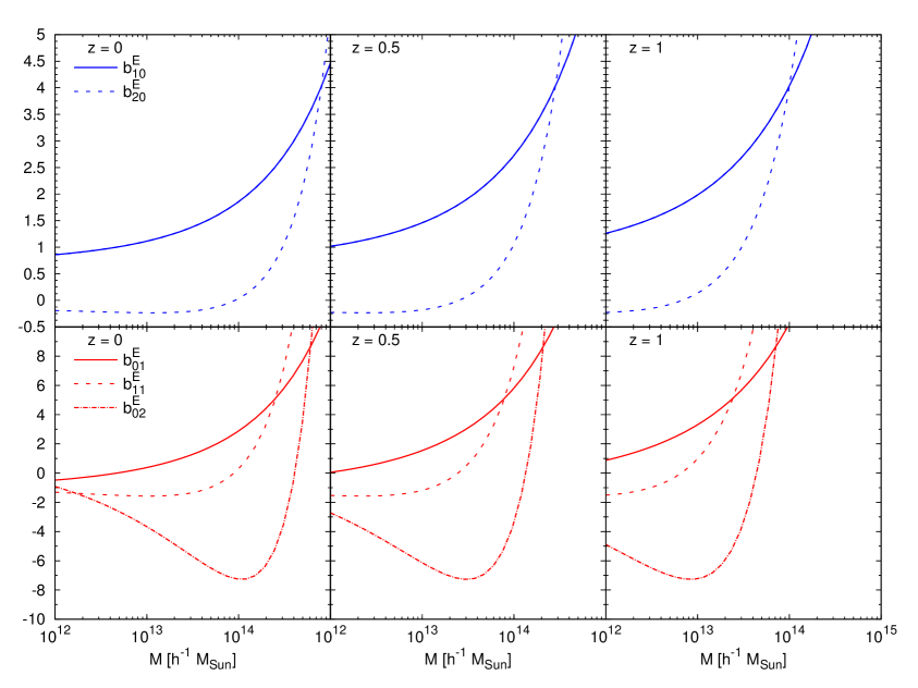
where we define the standard Eulerian bias coefficients (see fig. 2),

b10E=1+b10Lb01E=b01Lb20E=821b10L+b20Lb11E=b01L+b11Lb02E=b02L,superscriptsubscript𝑏10E1superscriptsubscript𝑏10Lsuperscriptsubscript𝑏01Esuperscriptsubscript𝑏01Lsuperscriptsubscript𝑏20E821superscriptsubscript𝑏10Lsuperscriptsubscript𝑏20Lsuperscriptsubscript𝑏11Esuperscriptsubscript𝑏01Lsuperscriptsubscript𝑏11Lsuperscriptsubscript𝑏02Esuperscriptsubscript𝑏02L\begin{split}b_{10}^{\rm E}&=1+b_{10}^{\rm L}\\ b_{01}^{\rm E}&=b_{01}^{\rm L}\\ b_{20}^{\rm E}&=\frac{8}{21}b_{10}^{\rm L}+b_{20}^{\rm L}\\ b_{11}^{\rm E}&=b_{01}^{\rm L}+b_{11}^{\rm L}\\ b_{02}^{\rm E}&=b_{02}^{\rm L}\,,\end{split} (4.7)

Equation 4.6 generalises the result that is usually obtained under the spherical collapse approximation (see appendix E). Indeed, the last two terms of eq. 4.6 are the non-local, non-linear terms of our bias model. While s2superscript𝑠2s^{2} is an already known tidal term, we have derived here for the first time the convective contribution 𝚿(𝐱,z)φG𝚿𝐱𝑧subscript𝜑G\mathbf{\Psi}(\mathbf{x},z)\cdot\mathbf{\nabla}\varphi_{\rm G}. We decide to keep the corresponding bias coefficients written as b10Lsuperscriptsubscript𝑏10Lb_{10}^{\rm L} and b01Lsuperscriptsubscript𝑏01Lb_{01}^{\rm L}, instead of replacing them with b10E1superscriptsubscript𝑏10E1b_{10}^{\rm E}-1 and b01Esuperscriptsubscript𝑏01Eb_{01}^{\rm E} respectively. In this way we will be able to recognise more easily the differences they introduce with respect to the reference model of BSS, especially in the discussion in section 6.
Refer to caption
Figure 2: The Eulerian bias coefficients as a function of mass and redshift, assuming fNL=1subscript𝑓NL1f_{\rm NL}=1.

Finally, if we perform a Fourier transform with respect to Euclidean coordinates we obtain

δhE(𝐤)=b10Eδ+b01EφG+b20Eδδ+b11EδφG+b02EφGφG27b10Ls2b01Ln2,superscriptsubscript𝛿E𝐤superscriptsubscript𝑏10E𝛿superscriptsubscript𝑏01Esubscript𝜑Gsuperscriptsubscript𝑏20E𝛿𝛿superscriptsubscript𝑏11E𝛿subscript𝜑Gsuperscriptsubscript𝑏02Esubscript𝜑Gsubscript𝜑G27superscriptsubscript𝑏10Lsuperscript𝑠2superscriptsubscript𝑏01Lsuperscript𝑛2\begin{split}\delta_{h}^{\rm E}(\mathbf{k})=\,&b_{10}^{\rm E}\delta+b_{01}^{\rm E}\varphi_{\rm G}+b_{20}^{\rm E}\delta\ast\delta+b_{11}^{\rm E}\delta\ast\varphi_{\rm G}+b_{02}^{\rm E}\varphi_{\rm G}\ast\varphi_{\rm G}-\frac{2}{7}b_{10}^{\rm L}s^{2}-b_{01}^{\rm L}n^{2}\,,\end{split} (4.8)

where we define

δE(𝐤)=superscript𝛿E𝐤absent\displaystyle\delta^{\rm E}(\mathbf{k})= δG(𝐤)+fNLα(k)d𝐪(2π)3δG(𝐪)δG(𝐤𝐪)α(q)α(|𝐤𝐪|)+d𝐪(2π)32(𝐪,𝐤𝐪)δG(𝐪)δG(𝐤𝐪)subscript𝛿G𝐤subscript𝑓NL𝛼𝑘𝑑𝐪superscript2𝜋3subscript𝛿G𝐪subscript𝛿G𝐤𝐪𝛼𝑞𝛼𝐤𝐪𝑑𝐪superscript2𝜋3subscript2𝐪𝐤𝐪subscript𝛿G𝐪subscript𝛿G𝐤𝐪\displaystyle\,\delta_{\rm G}(\mathbf{k})+f_{\rm NL}\alpha(k)\int\frac{d\mathbf{q}}{(2\pi)^{3}}\frac{\delta_{\rm G}(\mathbf{q})\delta_{\rm G}(\mathbf{k}-\mathbf{q})}{\alpha(q)\alpha(|\mathbf{k}-\mathbf{q}|)}+\int\,\frac{d\mathbf{q}}{(2\pi)^{3}}\mathcal{F}_{2}(\mathbf{q},\mathbf{k}-\mathbf{q})\delta_{\rm G}(\mathbf{q})\delta_{\rm G}(\mathbf{k}-\mathbf{q}) (4.9)
s2(𝐤)=superscript𝑠2𝐤absent\displaystyle s^{2}(\mathbf{k})= d𝐪(2π)3𝒮2(𝐪,𝐤𝐪)δG(𝐪)δG(𝐤𝐪)𝑑𝐪superscript2𝜋3subscript𝒮2𝐪𝐤𝐪subscript𝛿G𝐪subscript𝛿G𝐤𝐪\displaystyle\,\int\frac{d\mathbf{q}}{(2\pi)^{3}}\mathcal{S}_{2}(\mathbf{q},\mathbf{k}-\mathbf{q})\delta_{\rm G}(\mathbf{q})\delta_{\rm G}(\mathbf{k}-\mathbf{q}) (4.10)
n2(𝐤)=superscript𝑛2𝐤absent\displaystyle n^{2}(\mathbf{k})=  2d𝐪(2π)3𝒩2(𝐪,𝐤𝐪)δG(𝐪)δG(𝐤𝐪)α(|𝐤𝐪|)2𝑑𝐪superscript2𝜋3subscript𝒩2𝐪𝐤𝐪subscript𝛿G𝐪subscript𝛿G𝐤𝐪𝛼𝐤𝐪\displaystyle\,2\int\frac{d\mathbf{q}}{(2\pi)^{3}}\mathcal{N}_{2}(\mathbf{q},\mathbf{k}-\mathbf{q})\frac{\delta_{\rm G}(\mathbf{q})\delta_{\rm G}(\mathbf{k}-\mathbf{q})}{\alpha(|\mathbf{k}-\mathbf{q}|)} (4.11)

and the kernels are given by

2(𝐤1,𝐤2)subscript2subscript𝐤1subscript𝐤2\displaystyle\mathcal{F}_{2}(\mathbf{k}_{1},\mathbf{k}_{2}) =57+12𝐤1𝐤2k1k2(k1k2+k2k1)+27(𝐤1𝐤2)2k12k22absent5712subscript𝐤1subscript𝐤2subscript𝑘1subscript𝑘2subscript𝑘1subscript𝑘2subscript𝑘2subscript𝑘127superscriptsubscript𝐤1subscript𝐤22superscriptsubscript𝑘12superscriptsubscript𝑘22\displaystyle=\,\frac{5}{7}+\frac{1}{2}\frac{\mathbf{k}_{1}\cdot\mathbf{k}_{2}}{k_{1}k_{2}}\left(\frac{k_{1}}{k_{2}}+\frac{k_{2}}{k_{1}}\right)+\frac{2}{7}\frac{\left(\mathbf{k}_{1}\cdot\mathbf{k}_{2}\right)^{2}}{k_{1}^{2}k_{2}^{2}} (4.12)
𝒮2(𝐤1,𝐤2)subscript𝒮2subscript𝐤1subscript𝐤2\displaystyle\mathcal{S}_{2}(\mathbf{k}_{1},\mathbf{k}_{2}) =(𝐤1𝐤2)2k12k2213absentsuperscriptsubscript𝐤1subscript𝐤22superscriptsubscript𝑘12superscriptsubscript𝑘2213\displaystyle=\,\frac{\left(\mathbf{k}_{1}\cdot\mathbf{k}_{2}\right)^{2}}{k_{1}^{2}k_{2}^{2}}-\frac{1}{3} (4.13)
𝒩2(𝐤1,𝐤2)subscript𝒩2subscript𝐤1subscript𝐤2\displaystyle\mathcal{N}_{2}(\mathbf{k}_{1},\mathbf{k}_{2}) =𝐤1𝐤22k12.absentsubscript𝐤1subscript𝐤22superscriptsubscript𝑘12\displaystyle=\,\frac{\mathbf{k}_{1}\cdot\mathbf{k}_{2}}{2k_{1}^{2}}\,. (4.14)

The standard second-order Newtonian kernel 2subscript2\mathcal{F}_{2} is generated by the non-linear gravitational evolution. 𝒮2subscript𝒮2\mathcal{S}_{2} by the tidal term and the new kernel, 𝒩2subscript𝒩2\mathcal{N}_{2}, is generated by the convective term 𝚿φG𝚿subscript𝜑G\mathbf{\Psi}\cdot\mathbf{\nabla}\varphi_{\rm G}.

5 Three-point functions of halo and matter overdensities

In sections 5.1 and 5.2 we will present the tree-level bispectra for the halo and matter overdensities. We adopt the definition

δαE(𝐤1)δβE(𝐤2)δγE(𝐤3)=(2π)3δD(𝐤1+𝐤2+𝐤3)Bαβγ(𝐤1,𝐤2,𝐤3),delimited-⟨⟩subscriptsuperscript𝛿𝐸𝛼subscript𝐤1subscriptsuperscript𝛿𝐸𝛽subscript𝐤2subscriptsuperscript𝛿𝐸𝛾subscript𝐤3superscript2𝜋3superscript𝛿𝐷subscript𝐤1subscript𝐤2subscript𝐤3subscript𝐵𝛼𝛽𝛾subscript𝐤1subscript𝐤2subscript𝐤3\langle\delta^{E}_{\alpha}(\mathbf{k}_{1})\delta^{E}_{\beta}(\mathbf{k}_{2})\delta^{E}_{\gamma}(\mathbf{k}_{3})\rangle=(2\pi)^{3}\delta^{D}(\mathbf{k}_{1}+\mathbf{k}_{2}+\mathbf{k}_{3})B_{\alpha\beta\gamma}(\mathbf{k}_{1},\mathbf{k}_{2},\mathbf{k}_{3})\,, (5.1)

where α,β,γ=h,mformulae-sequence𝛼𝛽𝛾𝑚\alpha,\beta,\gamma=h,m with the labels hh and m𝑚m standing for halo and matter respectively. The crossed halo-matter bispectra are given in appendix G.

In sections 5.2 and 6 we will make use of the graphical representation introduced by Jeong and Komatsu [45] to show the shape dependence of the bispectrum. The amplitude of Bαβγsubscript𝐵𝛼𝛽𝛾B_{\alpha\beta\gamma}, or parts of it, will be plotted as a function of k2/k1subscript𝑘2subscript𝑘1k_{2}/k_{1} and k3/k1subscript𝑘3subscript𝑘1k_{3}/k_{1} in a colour map, under the condition k3k2k1subscript𝑘3subscript𝑘2subscript𝑘1k_{3}\leq k_{2}\leq k_{1}. This requirement avoids multiple visualizations of the same triangle. From all the possible choices of k2/k1subscript𝑘2subscript𝑘1k_{2}/k_{1} and k3/k1subscript𝑘3subscript𝑘1k_{3}/k_{1}, we can identify some specific configurations which are shown in fig. 3: equilateral (k1=k2=k3subscript𝑘1subscript𝑘2subscript𝑘3k_{1}=k_{2}=k_{3}), isosceles (k1>k2=k3subscript𝑘1subscript𝑘2subscript𝑘3k_{1}>k_{2}=k_{3} or k1=k2>k3subscript𝑘1subscript𝑘2subscript𝑘3k_{1}=k_{2}>k_{3}), folded (k1=2k2=2k3subscript𝑘12subscript𝑘22subscript𝑘3k_{1}=2k_{2}=2k_{3}), squeezed (k1k2k3similar-to-or-equalssubscript𝑘1subscript𝑘2much-greater-thansubscript𝑘3k_{1}\simeq k_{2}\gg k_{3}) and elongated (k1=k2+k3subscript𝑘1subscript𝑘2subscript𝑘3k_{1}=k_{2}+k_{3}).

Refer to caption
Figure 3: Explanation of the visual representation for the bispectrum introduced in [45]. The triangular-shaped region that hosts the colour map is due to the condition k3k2k1subscript𝑘3subscript𝑘2subscript𝑘1k_{3}\leq k_{2}\leq k_{1}. This requirement avoids double visualizations of the same triangular configuration. For the allowed values of k2/k1subscript𝑘2subscript𝑘1k_{2}/k_{1} and k3/k1subscript𝑘3subscript𝑘1k_{3}/k_{1} we recognise same specific configurations: point (a) is for the squeezed limit (k1k2k3similar-to-or-equalssubscript𝑘1subscript𝑘2much-greater-thansubscript𝑘3k_{1}\simeq k_{2}\gg k_{3}), (b) for the equilateral configuration (k1=k2=k3subscript𝑘1subscript𝑘2subscript𝑘3k_{1}=k_{2}=k_{3}) and (c) for the folded one (k1=2k2=2k3subscript𝑘12subscript𝑘22subscript𝑘3k_{1}=2k_{2}=2k_{3}). The elongated triangles (k1=k2+k3subscript𝑘1subscript𝑘2subscript𝑘3k_{1}=k_{2}+k_{3}) resides on the left edge, while the upper and right edges correspond to isosceles triangles (k1>k2=k3subscript𝑘1subscript𝑘2subscript𝑘3k_{1}>k_{2}=k_{3} or k1=k2>k3subscript𝑘1subscript𝑘2subscript𝑘3k_{1}=k_{2}>k_{3}). General configurations are in the inner region.

5.1 Matter bispectrum

The matter bispectrum is given from eqs. 4.9 and 5.1

Bmmm(𝐤1,𝐤2,𝐤3)=(2P(k1)P(k2)2(𝐤1,𝐤2)+2fNLP(k1)P(k2)α(k3)α(k1)α(k2)+2cyc.),subscript𝐵mmmsubscript𝐤1subscript𝐤2subscript𝐤32𝑃subscript𝑘1𝑃subscript𝑘2subscript2subscript𝐤1subscript𝐤22subscript𝑓NL𝑃subscript𝑘1𝑃subscript𝑘2𝛼subscript𝑘3𝛼subscript𝑘1𝛼subscript𝑘22cyc.B_{\text{mmm}}(\mathbf{k}_{1},\mathbf{k}_{2},\mathbf{k}_{3})=\left(2P(k_{1})P(k_{2})\mathcal{F}_{2}(\mathbf{k}_{1},\mathbf{k}_{2})+2f_{\rm NL}\frac{P(k_{1})P(k_{2})\alpha(k_{3})}{\alpha(k_{1})\alpha(k_{2})}+2\ \text{cyc.}\right)\,, (5.2)

where we have dropped the redshift z𝑧z dependence from the function α(k,z)𝛼𝑘𝑧\alpha(k,z) and the matter power spectrum P(k,z)𝑃𝑘𝑧P(k,z) in order to simplify the notation; we will do the same in the following sections. The matter bispectrum is thus generated by both primordial non-Gaussianity, fNLsubscript𝑓NLf_{\rm NL}, and non-linear gravitational evolution, 2subscript2\mathcal{F}_{2}.

The tree-level approximation based on perturbation theory well describes the simulation results at scales up to k0.050.1hMpc1similar-to-or-equals𝑘0.050.1superscriptMpc1k\simeq 0.05-0.1h\text{Mpc}^{-1}, depending on the redshift. Including one-loop corrections can significantly extend the validity for bispectrum to k0.3hMpc1similar-to-or-equals𝑘0.3superscriptMpc1k\simeq 0.3h\text{Mpc}^{-1} at redshift z1greater-than-or-equivalent-to𝑧1z\gtrsim 1 [68]. Alternatively, it is possible to use an effective kernel 2effsuperscriptsubscript2eff\mathcal{F}_{2}^{\rm eff} calibrated against simulations [87]. This phenomenological approach gives simpler expressions in the non-linear regime, and accurate predictions for the bispectrum, up to k0.4hMpc1similar-to-or-equals𝑘0.4superscriptMpc1k\simeq 0.4h\text{Mpc}^{-1} in the redshift range 0z1.50𝑧1.50\leq z\leq 1.5, when Gaussian initial conditions are assumed [88].

5.2 Halo bispectrum

First let us consider the halo bispectrum when Gaussian initial conditions (fNL=0subscript𝑓NL0f_{\rm NL}=0) are assumed [66]

BhhhG(𝐤1,𝐤2,𝐤3)=subscriptsuperscript𝐵𝐺hhhsubscript𝐤1subscript𝐤2subscript𝐤3absent\displaystyle B^{G}_{\text{hhh}}(\mathbf{k}_{1},\mathbf{k}_{2},\mathbf{k}_{3})= b103(2P(k1)P(k2)2(𝐤1,𝐤2)+2cyc.)Asuperscriptsubscript𝑏103subscript2𝑃subscript𝑘1𝑃subscript𝑘2subscript2subscript𝐤1subscript𝐤22cyc.A\displaystyle b_{10}^{3}\left(2P(k_{1})P(k_{2})\mathcal{F}_{2}(\mathbf{k}_{1},\mathbf{k}_{2})+2\ \text{cyc.}\right)_{\text{A}}
+\displaystyle+ b102b20(2P(k1)P(k2)+2cyc.)Lsuperscriptsubscript𝑏102subscript𝑏20subscript2𝑃subscript𝑘1𝑃subscript𝑘22cyc.L\displaystyle b_{10}^{2}b_{20}\left(2P(k_{1})P(k_{2})+2\ \text{cyc.}\right)_{\text{L}} (5.3)
\displaystyle- 27b102b10L(2P(k1)P(k2)𝒮2(𝐤1,𝐤2)+2cyc.)M.27superscriptsubscript𝑏102superscriptsubscript𝑏10Lsubscript2𝑃subscript𝑘1𝑃subscript𝑘2subscript𝒮2subscript𝐤1subscript𝐤22cyc.M\displaystyle\frac{2}{7}b_{10}^{2}b_{10}^{\rm L}\left(2P(k_{1})P(k_{2})\mathcal{S}_{2}(\mathbf{k}_{1},\mathbf{k}_{2})+2\ \text{cyc.}\right)_{\text{M}}\,.

Here and in the following the various terms appearing in the halo bispectrum are labelled in accordance with BSS [44] in order to facilitate comparison and to highlight the new terms we have identified. The halo bispectrum of section 5.2 is generated by the non-linear gravitational evolution, 2subscript2\mathcal{F}_{2}, by non-linear bias, b20subscript𝑏20b_{20}, and, in particular, the last term, 𝒮2subscript𝒮2\mathcal{S}_{2}, is due to the non-local tidal term, s2superscript𝑠2s^{2}, in the expression for the halo overdensity (see eq. 4.8). Note that, here and in the following, we have suppressed the E superscript in the bias factors to simplify the notation but not the L superscript. This allows to keep track of the effects generated by the non-local terms s2superscript𝑠2s^{2} and n2superscript𝑛2n^{2}.

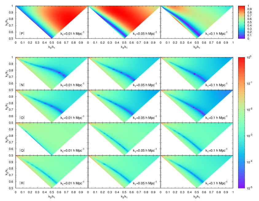
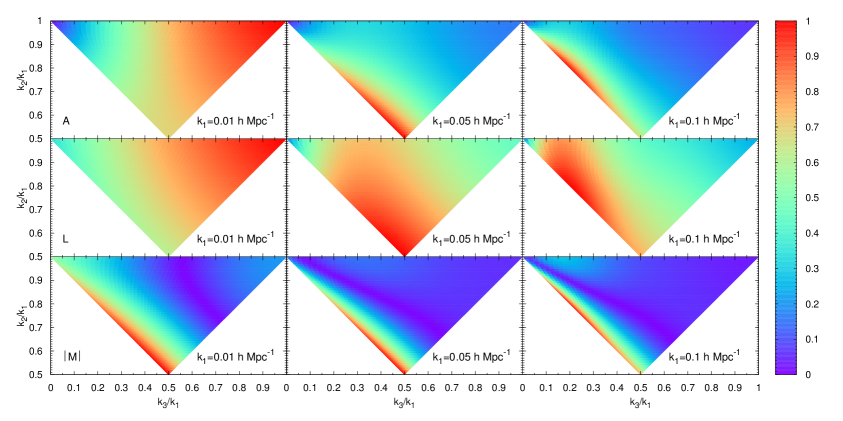
In fig. 4 we plot the shape dependence of each of the terms A,L,M for different choices of k1subscript𝑘1k_{1}, normalizing each of them to the maximum value it takes in the (k2/k1,k3/k1)subscript𝑘2subscript𝑘1subscript𝑘3subscript𝑘1(k_{2}/k_{1},k_{3}/k_{1})-space. This normalisation eliminates the redshift-dependence and as a result one should not make a comparison of the amplitude between plots because of the different scaling. The results are shown in fig. 4. Note that the absolute value is plotted for M, as it can be positive or negative. Indeed, the violet region that cuts the plots into two parts is where M changes sign.
Refer to caption
Figure 4: Shape dependence of the terms contributing to the halo bispectrum when Gaussian initial conditions are assumed and for k1=0.01,0.05,0.1hMpc1subscript𝑘10.010.050.1superscriptMpc1k_{1}=0.01,0.05,0.1h\text{Mpc}^{-1}. Each term is normalized to the maximum value it can take in the k2/k1subscript𝑘2subscript𝑘1k_{2}/k_{1},k3/k1subscript𝑘3subscript𝑘1k_{3}/k_{1}-space. This normalisation eliminates the redshift-dependence and as a result one should not make a comparison of the amplitude between plots because of the different scaling. Note that the last row shows the absolute value of M𝑀M, since it can take negative values. The violet strip indicates where it is changing sign.
Refer to caption
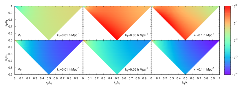
Figure 5: The term A is given by the sum of two pieces, which we label A1subscriptA1\text{A}_{1} and A2subscriptA2\text{A}_{2}. The former is sourced by non-linear gravitational evolution while the latter by PNG. We show them separately, normalized to the maximum value A can take and assuming z=0𝑧0z=0 and fNL=10subscript𝑓NL10f_{\rm NL}=10. The normalization does not completely cancel the redshift dependence, which is present in A2subscriptA2\text{A}_{2} through the factor D(z)1𝐷superscript𝑧1D(z)^{-1}. The effect of A2subscriptA2\text{A}_{2} is visible in the squeezed configuration, where A1subscriptA1\text{A}_{1} is vanishing and A2subscriptA2\text{A}_{2} is at its maximum (the logarithmic scale might hide this aspect but a quick look back to fig. 4 should clarify this point).

In the presence of primordial non-Gaussianity, many more terms contributes to the halo bispectrum:

Bhhh(𝐤1,𝐤2,𝐤3)=subscript𝐵hhhsubscript𝐤1subscript𝐤2subscript𝐤3absent\displaystyle B_{\text{hhh}}(\mathbf{k}_{1},\mathbf{k}_{2},\mathbf{k}_{3})= Bhhh(AL)(𝐤1,𝐤2,𝐤3)superscriptsubscript𝐵hhhALsubscript𝐤1subscript𝐤2subscript𝐤3\displaystyle B_{\text{hhh}}^{(\text{A}\rightarrow\text{L})}(\mathbf{k}_{1},\mathbf{k}_{2},\mathbf{k}_{3})
\displaystyle- 27b102b10L(2P(k1)P(k2)𝒮2(𝐤1,𝐤2)+2cyc.)M27superscriptsubscript𝑏102superscriptsubscript𝑏10Lsubscript2𝑃subscript𝑘1𝑃subscript𝑘2subscript𝒮2subscript𝐤1subscript𝐤22cyc.M\displaystyle\frac{2}{7}b_{10}^{2}b_{10}^{\rm L}\left(2P(k_{1})P(k_{2})\mathcal{S}_{2}(\mathbf{k}_{1},\mathbf{k}_{2})+2\ \text{cyc.}\right)_{\text{M}}
\displaystyle- 27b10b01b10L(2P(k1)P(k2)(1α(k1)+1α(k2))𝒮2(𝐤1,𝐤2)+2cyc.)N27subscript𝑏10subscript𝑏01superscriptsubscript𝑏10Lsubscript2𝑃subscript𝑘1𝑃subscript𝑘21𝛼subscript𝑘11𝛼subscript𝑘2subscript𝒮2subscript𝐤1subscript𝐤22cyc.N\displaystyle\frac{2}{7}b_{10}b_{01}b_{10}^{\rm L}\left(2P(k_{1})P(k_{2})\left(\frac{1}{\alpha(k_{1})}+\frac{1}{\alpha(k_{2})}\right)\mathcal{S}_{2}(\mathbf{k}_{1},\mathbf{k}_{2})+2\ \text{cyc.}\right)_{\text{N}}
\displaystyle- 27b012b10L(2P(k1)P(k2)α(k1)α(k2)𝒮2(𝐤1,𝐤2)+2cyc.)O27superscriptsubscript𝑏012superscriptsubscript𝑏10Lsubscript2𝑃subscript𝑘1𝑃subscript𝑘2𝛼subscript𝑘1𝛼subscript𝑘2subscript𝒮2subscript𝐤1subscript𝐤22cyc.O\displaystyle\frac{2}{7}b_{01}^{2}b_{10}^{\rm L}\left(2\frac{P(k_{1})P(k_{2})}{\alpha(k_{1})\alpha(k_{2})}\mathcal{S}_{2}(\mathbf{k}_{1},\mathbf{k}_{2})+2\ \text{cyc.}\right)_{\text{O}} (5.4)
\displaystyle- b102b01L(2P(k1)P(k2)(𝒩2(𝐤1,𝐤2)α(k2)+𝒩2(𝐤2,𝐤1)α(k1))+2cyc.)Psuperscriptsubscript𝑏102superscriptsubscript𝑏01Lsubscript2𝑃subscript𝑘1𝑃subscript𝑘2subscript𝒩2subscript𝐤1subscript𝐤2𝛼subscript𝑘2subscript𝒩2subscript𝐤2subscript𝐤1𝛼subscript𝑘12cyc.P\displaystyle b_{10}^{2}b_{01}^{\rm L}\left(2P(k_{1})P(k_{2})\left(\frac{\mathcal{N}_{2}(\mathbf{k}_{1},\mathbf{k}_{2})}{\alpha(k_{2})}+\frac{\mathcal{N}_{2}(\mathbf{k}_{2},\mathbf{k}_{1})}{\alpha(k_{1})}\right)+2\ \text{cyc.}\right)_{\text{P}}
\displaystyle- b10b01b01L(2P(k1)P(k2)(𝒩2(𝐤1,𝐤2)α(k2)+𝒩2(𝐤2,𝐤1)α(k1))(1α(k1)+1α(k2))+2cyc.)Qsubscript𝑏10subscript𝑏01superscriptsubscript𝑏01Lsubscript2𝑃subscript𝑘1𝑃subscript𝑘2subscript𝒩2subscript𝐤1subscript𝐤2𝛼subscript𝑘2subscript𝒩2subscript𝐤2subscript𝐤1𝛼subscript𝑘11𝛼subscript𝑘11𝛼subscript𝑘22cyc.Q\displaystyle b_{10}b_{01}b_{01}^{\rm L}\left(2P(k_{1})P(k_{2})\left(\frac{\mathcal{N}_{2}(\mathbf{k}_{1},\mathbf{k}_{2})}{\alpha(k_{2})}+\frac{\mathcal{N}_{2}(\mathbf{k}_{2},\mathbf{k}_{1})}{\alpha(k_{1})}\right)\left(\frac{1}{\alpha(k_{1})}+\frac{1}{\alpha(k_{2})}\right)+2\ \text{cyc.}\right)_{\text{Q}}
\displaystyle- b012b01L(2P(k1)P(k2)α(k1)α(k2)(𝒩2(𝐤1,𝐤2)α(k2)+𝒩2(𝐤2,𝐤1)α(k1))+2cyc.)R.superscriptsubscript𝑏012superscriptsubscript𝑏01Lsubscript2𝑃subscript𝑘1𝑃subscript𝑘2𝛼subscript𝑘1𝛼subscript𝑘2subscript𝒩2subscript𝐤1subscript𝐤2𝛼subscript𝑘2subscript𝒩2subscript𝐤2subscript𝐤1𝛼subscript𝑘12cyc.R\displaystyle b_{01}^{2}b_{01}^{\rm L}\left(2\frac{P(k_{1})P(k_{2})}{\alpha(k_{1})\alpha(k_{2})}\left(\frac{\mathcal{N}_{2}(\mathbf{k}_{1},\mathbf{k}_{2})}{\alpha(k_{2})}+\frac{\mathcal{N}_{2}(\mathbf{k}_{2},\mathbf{k}_{1})}{\alpha(k_{1})}\right)+2\ \text{cyc.}\right)_{\text{R}}\,.

The quantity Bhhh(AL)superscriptsubscript𝐵hhhALB_{\text{hhh}}^{(\text{A}\rightarrow\text{L})} accounts for the terms with label going from A to L; it matches exactly Eq.(5.1)5.1(5.1) of BSS, that we reproduce in appendix F.

The first line in eq. F.1, term A, comes from linear bias acting on the matter bispectrum. We can split this into two terms

A1(𝐤1,𝐤2,𝐤3)=subscriptA1subscript𝐤1subscript𝐤2subscript𝐤3absent\displaystyle\text{A}_{1}(\mathbf{k}_{1},\mathbf{k}_{2},\mathbf{k}_{3})= 2P(k1)P(k2)2(𝐤1,𝐤2)+2cyc.2𝑃subscript𝑘1𝑃subscript𝑘2subscript2subscript𝐤1subscript𝐤22cyc.\displaystyle 2P(k_{1})P(k_{2})\mathcal{F}_{2}(\mathbf{k}_{1},\mathbf{k}_{2})+2\ \text{cyc.} (5.5)
A2(k1,k2,k3)=subscriptA2subscript𝑘1subscript𝑘2subscript𝑘3absent\displaystyle\text{A}_{2}(k_{1},k_{2},k_{3})= 2fNLP(k1)P(k2)α(k3)α(k1)α(k2)+2cyc.,2subscript𝑓NL𝑃subscript𝑘1𝑃subscript𝑘2𝛼subscript𝑘3𝛼subscript𝑘1𝛼subscript𝑘22cyc.\displaystyle 2f_{\rm NL}\frac{P(k_{1})P(k_{2})\alpha(k_{3})}{\alpha(k_{1})\alpha(k_{2})}+2\ \text{cyc.}\,, (5.6)

identifying an additional term, A2subscriptA2\text{A}_{2}, with respect to the Gaussian initial conditions section 5.2 proportional to fNLsubscript𝑓NLf_{\rm NL}. We study the shape dependence of A1subscriptA1\text{A}_{1} and A2subscriptA2\text{A}_{2} in fig. 5. Again, we plot them separately but normalize to the maximum value taken by A(𝐤1,𝐤2,𝐤3)=A1+A2Asubscript𝐤1subscript𝐤2subscript𝐤3subscriptA1subscriptA2\text{A}(\mathbf{k}_{1},\mathbf{k}_{2},\mathbf{k}_{3})=\text{A}_{1}+\text{A}_{2} in the k2/k1subscript𝑘2subscript𝑘1k_{2}/k_{1},k3/k1subscript𝑘3subscript𝑘1k_{3}/k_{1}-space. The relative values of the two plots can thus be compared, but note that the normalization does not cancel the growth factor 1/α1/D(z)proportional-to1𝛼1𝐷𝑧1/\alpha\propto 1/D(z) in A2subscriptA2\text{A}_{2} but absent in A1subscriptA1\text{A}_{1}. Hence the relative amplitude of the bispectrum from primordial non-Gaussianity A2subscriptA2\text{A}_{2} grows with redshift relative the bispectrum A1subscriptA1\text{A}_{1} coming from Gaussian initial conditions. Figure 5 highlights the interesting shape dependence of A2subscriptA2\text{A}_{2}; it peaks in the extremely squeezed configuration (top left), exactly where the A1subscriptA1\text{A}_{1} term vanishes (see also fig. 4).

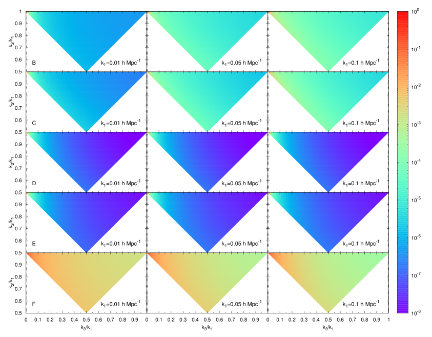
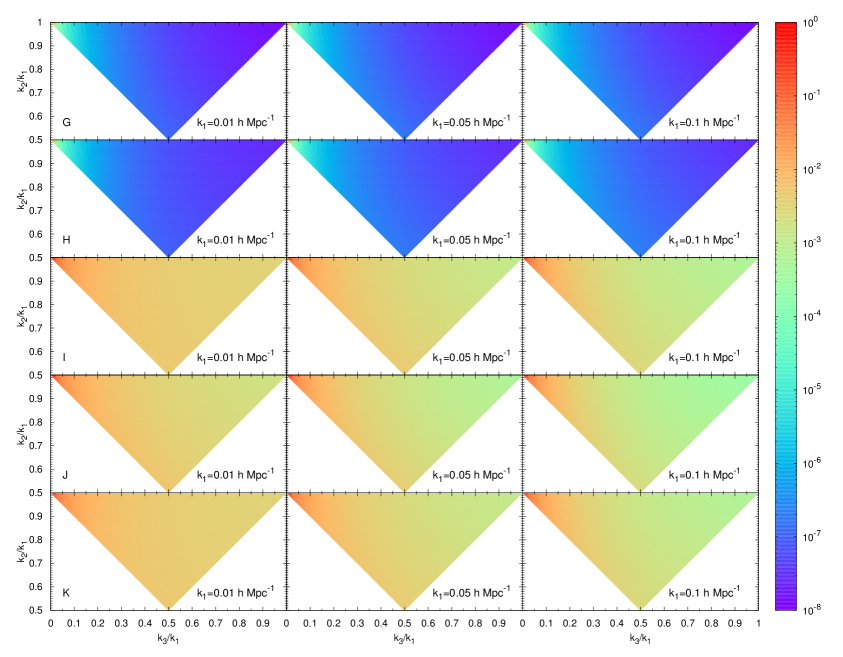
We emphasize that A2subscriptA2\text{A}_{2} and the terms from B to K are generated by primordial non-Gaussianity. We plot the shape dependence of the terms B to F in fig. 6 and the term G to K in fig. 7. They confirm what we have previously stated: the PNG terms are greatest in the squeezed configuration.
Refer to caption
Figure 6: Shape dependence of the terms, B to F, contributing to the halo bispectrum. These are generated by non-Gaussian initial conditions. A value fNL=10subscript𝑓NL10f_{\rm NL}=10 and redshift z=0𝑧0z=0 are assumed. Each term is normalized to the maximum it can take. This choice does not completely cancel the redshift dependence in the terms B and C, where it is present as a factor D(z)1𝐷superscript𝑧1D(z)^{-1}, and does not allow a comparison of the amplitude between different plots. We clearly see that the effect of PNG is prominent in the squeezed configuration.
Refer to caption
Figure 7: The terms contributing to the halo bispectrum, with label going from G to K. These are generated by non-Gaussian initial conditions. A value fNL=10subscript𝑓NL10f_{\rm NL}=10 is assumed. Each term is normalized to the maximum it can take. This choice completely cancels the redshift dependence and does not allow a comparison of the amplitude between different terms. We clearly see that the effect of PNG is prominent in the squeezed configuration.

As a result of the presence of s2superscript𝑠2s^{2} and our new term n2superscript𝑛2n^{2} in the expression for δhEsuperscriptsubscript𝛿E\delta_{h}^{\rm E} (see eq. 4.8), additional terms appear with respect to BSS. M, N and O that are generated by the tidal term s2superscript𝑠2s^{2}; schematically, they are sourced by s2δδdelimited-⟨⟩superscript𝑠2𝛿𝛿\langle s^{2}\delta\delta\rangle, s2δφdelimited-⟨⟩superscript𝑠2𝛿𝜑\langle s^{2}\delta\varphi\rangle and s2φφdelimited-⟨⟩superscript𝑠2𝜑𝜑\langle s^{2}\varphi\varphi\rangle respectively. We have seen in section 5.2 that M is present regardless of the presence of PNG, but N and O come from the coupling between the tidal term and φGsubscript𝜑G\varphi_{\rm G} for fNL0subscript𝑓NL0f_{\rm NL}\neq 0. On the other hand, P, Q and R are generated by n2superscript𝑛2n^{2}. They account for the non-local effect of the potential φGsubscript𝜑G\varphi_{\rm G} and are therefore due to the presence of PNG. Schematically, they are generated by n2δδdelimited-⟨⟩superscript𝑛2𝛿𝛿\langle n^{2}\delta\delta\rangle, n2δφdelimited-⟨⟩superscript𝑛2𝛿𝜑\langle n^{2}\delta\varphi\rangle, n2φφdelimited-⟨⟩superscript𝑛2𝜑𝜑\langle n^{2}\varphi\varphi\rangle respectively. In fig. 8 we show the terms from N to R. Since they can take negative values, we plot their absolute value. Interestingly, in all of the plots we can identify a violet strip, indicating a change of sign and, hence, where the kernels 𝒮2subscript𝒮2\mathcal{S}_{2} and 𝒩2subscript𝒩2\mathcal{N}_{2} make each term vanish.

Refer to caption
Figure 8: Shape dependence of the terms with label going from N to R contributing to the halo bispectrum. These are the additional terms generated by the presence of s2superscript𝑠2s^{2} and n2superscript𝑛2n^{2} in δhsubscript𝛿\delta_{h}. A value fNL=10subscript𝑓NL10f_{\rm NL}=10 is assumed. Each term is normalized to maximum value it can take so that the redshift dependence is completely dropped; note however that the different scaling does not allow one to compare the amplitude between plots. Since these terms can take negative values, we show their absolute value. Actually, the blue line indicates where they change sign, with the top right part of the plots being positive.

6 Analytic estimates

In this section we further investigate our result for the halo bispectrum and, in particular, we compare it to our reference model BSS [44]. Since the model of BSS has shown a good fit against simulations [44, 89], we want to understand if and where differences between these two models arise.

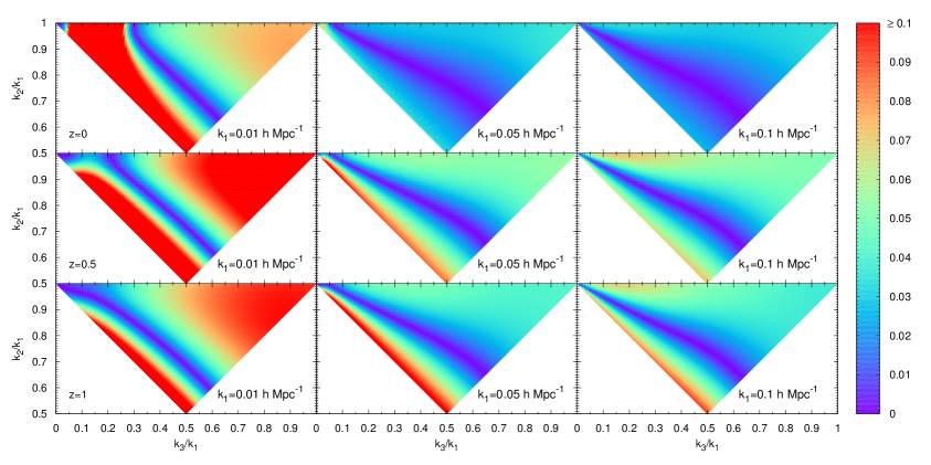
In fig. 9 we plot the absolute value of the relative difference between our halo bispectrum and that of BSS

Diff(𝐤1,𝐤2,𝐤3)=|BTRTW(𝐤1,𝐤2,𝐤3)BBSS(𝐤1,𝐤2,𝐤3)BBSS(𝐤1,𝐤2,𝐤3)|,\text{Diff}(\mathbf{k}_{1},\mathbf{k}_{2},\mathbf{k}_{3})=\Biggr{|}\frac{B_{\text{TRTW}}(\mathbf{k}_{1},\mathbf{k}_{2},\mathbf{k}_{3})-B_{\text{BSS}}(\mathbf{k}_{1},\mathbf{k}_{2},\mathbf{k}_{3})}{B_{\text{BSS}}(\mathbf{k}_{1},\mathbf{k}_{2},\mathbf{k}_{3})}\Biggr{|}\,, (6.1)

for values of k1=0.01,0.05,0.1hMpc1subscript𝑘10.010.050.1superscriptMpc1k_{1}=0.01,0.05,0.1h\text{Mpc}^{-1} and redshift z=0,0.5,1𝑧00.51z=0,0.5,1. We consider halos of mass M=1013h1M𝑀superscript1013superscripth1subscript𝑀direct-productM=10^{13}\text{h}^{-1}M_{\odot} and primordial non-Gaussianity with fNL=10subscript𝑓NL10f_{\rm NL}=10.

Refer to caption
Figure 9: The relative difference in absolute value between our model and the one by Baldauf et al., assuming M=1013h1M𝑀superscript1013superscript1subscript𝑀direct-productM=10^{13}h^{-1}M_{\odot} and fNL=10subscript𝑓NL10f_{\rm NL}=10. Note that we saturate differences above 10%percent1010\% to the same red colour of the palette; as the plots range between different values, this choice allows us to present them in a compact way, highlighting where the most relevant differences are expected. However we do not observe discrepancies above 25%percent2525\%. Interestingly, the squeezed limit is not affected while the other configurations show differences from only a few percent. A no-difference region going approximately from the squeezed to the isosceles configurations is present, following the shape dependence that we showed in figs. 4 and 8.

We choose to saturate differences above 10%percent1010\% to the same red colour of the palette for the purpose of presenting many different plots with different ranges of values in a compact way. However we do not observe differences above 25%percent2525\% 666An exception is the top left plot of fig. 9, where there is a small curve close to the squeezed configuration in which the discrepancy is actually bigger than that. This because in that area the BSS halo bispectrum crosses zero for these values of the bias coefficients. .

For the value of the halo mass and fNLsubscript𝑓NLf_{\rm NL} considered, we find that the terms M and P are the main sources of the differences, with all the other terms contributing very little or having a negligible effect. The most relevant differences appear for k1=0.01hMpc1subscript𝑘10.01superscriptMpc1k_{1}=0.01h\text{Mpc}^{-1}: up to 25%percent2525\% in the elongated, folded and equilateral regions for all the redshifts considered. These discrepancies drop to a few percent for k1=0.05hMpc1subscript𝑘10.05superscriptMpc1k_{1}=0.05h\text{Mpc}^{-1} at z=0𝑧0z=0, while for z=0.5,1𝑧0.51z=0.5,1 they are reduced to about 5%percent55\% when approaching the equilateral configuration and to order 10%percent1010\% in the elongated and folded regions. For k1=0.1hMpc1subscript𝑘10.1superscriptMpc1k_{1}=0.1h\text{Mpc}^{-1} we observe a similar pattern, but at z=0.5𝑧0.5z=0.5 the approximately 10%percent1010\% difference area that was present in the elongated and folded regions for k1=0.05hMpc1subscript𝑘10.05superscriptMpc1k_{1}=0.05h\text{Mpc}^{-1} is almost completely washed out, decreased to about 5%percent55\%. However, that area is still present for z=1𝑧1z=1, although reduced in size. We also recognise an area where the difference is close to zero [the violet region going approximately from the squeezed (top left) to the isosceles (bottom right) configuration] corresponding to a vanishing contribution from the terms M to R, as shown in figs. 4 and 8. Interestingly, in all plots the squeezed configuration is unaffected.

We can understand the features that we have just described by studying the analytic solutions of the halo bispectrum in three simple configurations:

  • In the equilateral configuration, where k1=k2=k3=ksubscript𝑘1subscript𝑘2subscript𝑘3𝑘k_{1}=k_{2}=k_{3}=k, the halo bispectrum becomes

    Bhhh=subscript𝐵hhhabsent\displaystyle B_{\text{hhh}}= {b1027(12b10+b10L+42b20)\displaystyle\Biggr{\{}\frac{b_{10}^{2}}{7}(12b_{10}+b_{10}^{\rm L}+42b_{20})
    +1α(k)[27b01b10(12b10+b10L+42b20)+3b102(b01L+2(fNLb10+b11))]\displaystyle+\frac{1}{\alpha(k)}\biggr{[}\frac{2}{7}b_{01}b_{10}\bigr{(}12b_{10}+b_{10}^{\rm L}+42b_{20}\bigr{)}+3b_{10}^{2}\biggr{(}b_{01}^{\rm L}+2\bigr{(}f_{\rm NL}b_{10}+b_{11}\bigr{)}\biggr{)}\biggr{]}
    +1α(k)2[b0127(12b10+b10L+42b20)+6b01b10(b01L+2(fNLb10+b11))+6b02b102]\displaystyle+\frac{1}{\alpha(k)^{2}}\biggr{[}\frac{b_{01}^{2}}{7}\bigr{(}12b_{10}+b_{10}^{\rm L}+42b_{20}\bigr{)}+6b_{01}b_{10}\biggr{(}b_{01}^{\rm L}+2\bigr{(}f_{\rm NL}b_{10}+b_{11}\bigr{)}\biggr{)}+6b_{02}b_{10}^{2}\biggr{]}
    +3α(k)3[b012(b01L+2(fNLb10+b11))+84b01b02b10]+6b012b02α(k)4}P(k)2\displaystyle+\frac{3}{\alpha(k)^{3}}\biggr{[}b_{01}^{2}\biggr{(}b_{01}^{\rm L}+2\bigr{(}f_{\rm NL}b_{10}+b_{11}\bigr{)}\biggr{)}+84b_{01}b_{02}b_{10}\biggr{]}+\frac{6b_{01}^{2}b_{02}}{\alpha(k)^{4}}\Biggr{\}}P(k)^{2} (6.2)

    We remind the reader that the contributions of b10Lsuperscriptsubscript𝑏10Lb_{10}^{\rm L} and b01Lsuperscriptsubscript𝑏01Lb_{01}^{\rm L} indicate where the non-local, non-linear terms of our model (s2superscript𝑠2s^{2} and n2superscript𝑛2n^{2}) are introducing differences respect to the BSS model. By looking at eq. 5.4 we notice that the terms M, N, O, P, Q, R are respectively linked to the bias combinations b102b10Lsuperscriptsubscript𝑏102superscriptsubscript𝑏10Lb_{10}^{2}b_{10}^{\rm L}, b10b01b10Lsubscript𝑏10subscript𝑏01superscriptsubscript𝑏10Lb_{10}b_{01}b_{10}^{\rm L}, b012b10Lsuperscriptsubscript𝑏012superscriptsubscript𝑏10Lb_{01}^{2}b_{10}^{\rm L}, b102b01Lsuperscriptsubscript𝑏102superscriptsubscript𝑏01Lb_{10}^{2}b_{01}^{\rm L}, b10b01b01Lsubscript𝑏10subscript𝑏01superscriptsubscript𝑏01Lb_{10}b_{01}b_{01}^{\rm L}, b012b01Lsuperscriptsubscript𝑏012superscriptsubscript𝑏01Lb_{01}^{2}b_{01}^{\rm L}, so that we can actually recognize each of them in section 6; M appears in the first line of section 6, while N and P appear in the second line, O and Q in the third and R in the first term on the fourth line.

    The presence of a larger difference at high redshift and on large scales can be explained by noting that the function α(k)𝛼𝑘\alpha(k) takes smaller values in those regimes and enhances the terms inside the square brackets (see eq. 2.3 and fig. 1) and, therefore, accentuates the effect of b10Lsuperscriptsubscript𝑏10Lb_{10}^{\rm L} and b01Lsuperscriptsubscript𝑏01Lb_{01}^{\rm L}.

  • In the folded configuration, k2=k3=ksubscript𝑘2subscript𝑘3𝑘k_{2}=k_{3}=k and k1=2ksubscript𝑘12𝑘k_{1}=2k, the halo bispectrum can be written as

    Bhhh=subscript𝐵hhhabsent\displaystyle B_{\text{hhh}}= {2b103(2Π2)+b102(2b20821b10L)(1+4Π2)+\displaystyle\Biggr{\{}2b_{10}^{3}\left(2-\Pi^{2}\right)+b_{10}^{2}\left(2b_{20}-\frac{8}{21}b_{10}^{\rm L}\right)\left(1+4\Pi^{2}\right)+
    +1α(k)[10b103fNLΠ2+b102(b01(8Π22Π2)+2b01L(1+Π+Π2)+b11(2+Π+4Π2))\displaystyle+\frac{1}{\alpha(k)}\biggr{[}10b_{10}^{3}f_{\rm NL}\Pi^{2}+b_{10}^{2}\biggr{(}b_{01}\left(8-\frac{\Pi}{2}-2\Pi^{2}\right)+2b_{01}^{\rm L}\left(-1+\Pi+\Pi^{2}\right)+b_{11}\left(2+\Pi+4\Pi^{2}\right)\biggr{)}
    +b10(2b01b20821b01b10L)(2+Π+4Π)]\displaystyle+b_{10}\left(2b_{01}b_{20}-\frac{8}{21}b_{01}b_{10}^{\rm L}\right)\left(2+\Pi+4\Pi\right)\biggr{]}
    +1α(k)2[]+1α(k)3[]+1α(k)4[]}P(k)2.\displaystyle+\frac{1}{\alpha(k)^{2}}\biggr{[}\dots\biggr{]}+\frac{1}{\alpha(k)^{3}}\biggr{[}\dots\biggr{]}+\frac{1}{\alpha(k)^{4}}\biggr{[}\dots\biggr{]}\Biggr{\}}P(k)^{2}\,. (6.3)

    where we define Π=T(2k)/T(k)Π𝑇2𝑘𝑇𝑘\Pi=T(2k)/T(k) to make the notation more compact. The full expression is long so we have given just the first two terms. These are enough to explain what we observe in fig. 9. Again, b10Lsuperscriptsubscript𝑏10Lb_{10}^{\rm L} and b01Lsuperscriptsubscript𝑏01Lb_{01}^{\rm L} are present. As for the equilateral configuration, the effect of M appears in the first term, while N and P in the second one, O and Q in the third and R in the fourth one. We see that the effect of b10Lsuperscriptsubscript𝑏10Lb_{10}^{\rm L} and b01Lsuperscriptsubscript𝑏01Lb_{01}^{\rm L} can be enhanced depending on the value of ΠΠ\Pi. When k1=0.01hMpcsubscript𝑘10.01Mpck_{1}=0.01h\text{Mpc} the ratio Π1Π1\Pi\approx 1, while for the other two values of k1subscript𝑘1k_{1} the ratio Π<1Π1\Pi<1. This suggests why bigger differences should be expected in the case with k1=0.01hMpcsubscript𝑘10.01Mpck_{1}=0.01h\text{Mpc}.

    The same considerations apply to the function α(k)𝛼𝑘\alpha(k) as in the equilateral case, so that the differences are larger at high redshift and on large scales.

  • A simple expression for the halo bispectrum in the squeezed limit can be found by setting k1=k2=ϵk3=ksubscript𝑘1subscript𝑘2italic-ϵsubscript𝑘3𝑘k_{1}=k_{2}=\epsilon k_{3}=k with ϵ1much-greater-thanitalic-ϵ1\epsilon\gg 1, corresponding to an isosceles triangle, whose degree of squeezing is controlled by the parameter ϵitalic-ϵ\epsilon. For squeezed triangles (large values of ϵitalic-ϵ\epsilon), the leading term in the bispectrum is

    Bhhhsubscript𝐵hhhabsent\displaystyle B_{\text{hhh}}\approx [2α(k)2(2fNLb01b102+b01b10b11)+2α(k)3(2fNLb012b10+b012b11+2b01b02b10)\displaystyle\Biggr{[}\frac{2}{\alpha(k)^{2}}\biggr{(}2f_{\rm NL}b_{01}b_{10}^{2}+b_{01}b_{10}b_{11}\biggr{)}+\frac{2}{\alpha(k)^{3}}\biggr{(}2f_{\rm NL}b_{01}^{2}b_{10}+b_{01}^{2}b_{11}+2b_{01}b_{02}b_{10}\biggr{)}
    +4α(k)4b012b02]P(k)2ϵ3.\displaystyle+\frac{4}{\alpha(k)^{4}}b_{01}^{2}b_{02}\Biggr{]}P(k)^{2}\epsilon^{3}\,. (6.4)

    The absence of terms involving bias coefficients b10Lsuperscriptsubscript𝑏10Lb_{10}^{\rm L} and b01Lsuperscriptsubscript𝑏01Lb_{01}^{\rm L} explains why our predictions do not differ from the BSS model in extremely squeezed configurations.

7 Conclusions

An important application of measurements of large-scale structure in our Universe is to determine the distribution of primordial perturbations, in particular possible non-Gaussian signatures of scenarios for the origin of structure in the very early universe. For example, the shape information contained in the primordial bispectrum is a valuable tool to discriminate between different inflationary models. The matter bispectrum at later times is due to a combination of both primordial non-Gaussianity and non-linear evolution under gravity. However, the way in which gravitationally collapsed halos trace the density field, the bias model, can enhance the effect of primordial non-Gaussianity in the galaxy distribution. In particular, local-type non-Gaussianity leads to a scale-dependent bias which can have a dramatic effect on very large scales in both the halo power spectrum [8, 9] and the halo bispectrum [46].

In this paper we developed a local Lagrangian bias model, focussing on second-order, non-local and non-Gaussian effects. In particular, we extended and applied a local Lagrangian biasing scheme to a general set-up with local-type primordial non-Gaussianity. For an fNLsubscript𝑓NLf_{\rm NL} cosmology, we re-derive the known result [67] that the halo overdensity can be expressed as a bivariate expansion in terms of the linear matter overdensity in the Lagrangian frame and the primordial Gaussian potential.

Non-linear evolution of the matter field in general gives rise to second-order terms in the matter density which include non-local, tidal terms (see eq. 2.8), while transforming from the Lagrangian to the Eulerian frame introduces a non-local convective term at second order (see eq. 2.12). Non-local here implies terms derived from derivatives of the potential, not directly from the local density or its derivatives. Both these terms are included in the usual kernel, 2subscript2\mathcal{F}_{2}, for the second-order density in Eulerian space. But since the halo density is determined by the linear matter overdensity in the Lagrangian frame, one must account separately for these non-local terms to reconstruct the halo density at late times. These terms are absent at early times, or if we restrict ourselves to the spherical collapse approximation (see appendix E).

We have shown in this paper that in the bivariate expansion we must also account at second order for the convective term relating the primordial potential in the Lagrangian frame to that in Eulerian space at later times (see eq. 2.13). This gives rise to a new term in the halo bispectrum in the presence of local-type primordial non-Gaussianity which has not previously been studied as far as we are aware.

Setting fNL=0subscript𝑓NL0f_{\rm NL}=0 and are able to recover the halo bispectrum model of [66], when a local Lagrangian biasing scheme is applied. Three terms appear in the halo bispectrum (A,L and M) that are sourced by (A) the non-linear matter density encoded in the kernel 2subscript2\mathcal{F}_{2}, (L) the non-linear bias b20subscript𝑏20b_{20} and (M) the tidal term s2superscript𝑠2s^{2}.

Generalising to fNL0subscript𝑓NL0f_{\rm NL}\neq 0, we found 121212 terms in the halo bispectrum (labelled A to L) matching the BSS model [44]. In this case, the non-linear matter density term, A, includes a correction due to PNG, while the non-linear bias term, L, is left unchanged. The other contributions (B to K) come from a mixture of bivariate terms, involving the bias coefficients b01subscript𝑏01b_{01}, b11subscript𝑏11b_{11}, b02subscript𝑏02b_{02}. We also found a contribution, M, sourced by the tidal term, s2superscript𝑠2s^{2}, which also couples with terms in the halo overdensity that are specifically due to PNG and, hence, generate new contributions, N and O, in the halo bispectrum. The new convective term, n2superscript𝑛2n^{2}, also generates contributions in the presence of primordial non-Gaussianity; in the halo bispectrum we have found three new contributions, P, Q and R, due to this term.

In order to investigate the magnitude and shape of the various contributions to the bispectrum, we have implemented a version of the Sheth-Tormen mass function corrected for PNG in light of the Lo Verde mass function, following BSS [44]. This allowed us to numerically calculate the bias coefficients for our model and predict the halo bispectrum in different configurations for sample values of fNLsubscript𝑓NLf_{\rm NL} and at various scales and redshifts.

We investigated the halo bispectrum by comparing it to the fiducial model of BSS. Assuming halos of mass M=1013h1MMsuperscript1013superscript1subscriptMdirect-product{\rm M}=10^{13}h^{-1}{\rm M}_{\odot} and fNL=10subscript𝑓NL10f_{\rm NL}=10, we found:

  • -

    At redshift z=0𝑧0z=0 differences up to 25%percent2525\% in the halo bispectrum for k1=0.01hMpc1subscript𝑘10.01superscriptMpc1k_{1}=0.01h\text{Mpc}^{-1} in the elongated and folded configurations and approximately 78%7percent87-8\% when approaching the equilateral configuration, while these drop to a few percent when k1=0.05subscript𝑘10.05k_{1}=0.05 or 0.1hMpc10.1superscriptMpc10.1h\text{Mpc}^{-1}.

  • -

    At redshift z=0.5𝑧0.5z=0.5 differences up to 25%percent2525\% for k1=0.01hMpc1subscript𝑘10.01superscriptMpc1k_{1}=0.01h\text{Mpc}^{-1} in the elongated, folded and equilateral configurations. When k1=0.05hMpc1subscript𝑘10.05superscriptMpc1k_{1}=0.05h\text{Mpc}^{-1} differences of order 10%percent1010\% are still visible in the elongated and folded shapes, while they decrease to approximately 5%percent55\% towards the equilateral configuration. For k1=0.1hMpc1subscript𝑘10.1superscriptMpc1k_{1}=0.1h\text{Mpc}^{-1} these differences reduce to about 5%percent55\%.

  • -

    At redshift z=1𝑧1z=1 we find results similar to those for z=0.5𝑧0.5z=0.5, except that differences of order 10%percent1010\% are still visible in the elongated and folded regions for k1=0.1hMpc1subscript𝑘10.1superscriptMpc1k_{1}=0.1h\text{Mpc}^{-1}.

In general, we observe that the non-local terms have a negligible effect in extremely squeezed configurations.

Our results indicate that the non-local terms in the halo overdensity could have a significant contribution to the galaxy bispectrum, especially on large scales and at high redshift. The next challenge is to test these theoretical predictions against N-body simulations with non-Gaussian initial conditions. Ultimately we would wish to be able to estimate the signal-to-noise for upcoming surveys, like the ESA Euclid mission [90], which probes large scales and high redshifts, in order to explore the observability of these non-local effects in the bispectrum. A full discussion of the observability of these effects must include a halo occupation model, to describe how galaxies populate halos and many other effects including redshift space distortions and lensing along the line of sight, from galaxies to the observer, in order to translate theoretical model for the halo bispectrum into predictions for the observed galaxy angular bispectrum in redshift space. Nonetheless, we have identified in this paper novel contributions to the expected galaxy bispectrum on large scales and high redshift in the presence of primordial non-Gaussianity.

Acknowledgments

The authors wish to thank Cornelius Rampf for help in the early stages of this work and Tommaso Giannantonio, Nina Roth, Jennifer E. Pollack for many helpful discussions. They are also grateful to Kazuya Koyama for carefully reading the paper and providing many useful comments. MT acknowledges Tobias Baldauf for email communication and Vincent Desjacques, Héctor Gil-Marín, Francesco Pace and Sandro Ciarlariello for useful discussions. GT is supported by an STFC Advanced Fellowship ST/H005498/1. DW is supported by STFC grants ST/K00090X/1 and ST/L005573/1.

Appendix A Displaced Gaussian random fields

In deriving the halo abundance in Eulerian space we need to map the initial gravitational potential in Lagrangian coordinates, eq. 2.4, into Eulerian coordinates under the coordinate displacement eq. 1.3, which is itself determined by the gravitational potential. In this appendix we shall demonstrate how even an initial Gaussian field in Lagrangian coordinates may be transformed into a non-Gaussian field by this displacement to Eulerian coordinates.

We start from a random field, φ^G(q)subscript^𝜑𝐺𝑞\hat{\varphi}_{G}(q), defined with respect to the Lagrangian coordinate chart, q𝑞q. Let

φ^G(q)=ϵf(q)a^,subscript^𝜑𝐺𝑞italic-ϵ𝑓𝑞^𝑎\hat{\varphi}_{G}(q)=\epsilon f(q)\hat{a}\,, (A.1)

where a^^𝑎\hat{a} denotes a Gaussian random variable and ϵitalic-ϵ\epsilon is a small perturbative parameter. Thus φ^G(q)subscript^𝜑𝐺𝑞\hat{\varphi}_{G}(q) is a Gaussian random field (first order with respect to ϵitalic-ϵ\epsilon) with, for example, vanishing 3-point function

φ^G(q1)φ^G(q2)φ^G(q3)=ϵ3f(q1)f(q2)f(q3)a^3=0.delimited-⟨⟩subscript^𝜑𝐺subscript𝑞1subscript^𝜑𝐺subscript𝑞2subscript^𝜑𝐺subscript𝑞3superscriptitalic-ϵ3𝑓subscript𝑞1𝑓subscript𝑞2𝑓subscript𝑞3delimited-⟨⟩superscript^𝑎30\langle\hat{\varphi}_{G}(q_{1})\hat{\varphi}_{G}(q_{2})\hat{\varphi}_{G}(q_{3})\rangle=\epsilon^{3}f(q_{1})f(q_{2})f(q_{3})\langle\hat{a}^{3}\rangle=0\,. (A.2)

where angle-brackets denote the ensemble average.

Let the Eulerian coordinate x𝑥x be related to q𝑞q by a first-order displacement field ψ^(q)^𝜓𝑞\hat{\psi}(q), correlated with the field φ^Gsubscript^𝜑𝐺\hat{\varphi}_{G} such that

x^(q)=q+ϵψ(q)a^.^𝑥𝑞𝑞italic-ϵ𝜓𝑞^𝑎\hat{x}(q)=q+\epsilon\psi(q)\hat{a}\,. (A.3)

If we consider a fixed coordinate q𝑞q then x^(q)^𝑥𝑞\hat{x}(q) is itself a random variable, correlated with φ^G(q)subscript^𝜑𝐺𝑞\hat{\varphi}_{G}(q). We can then construct the field

φ^G(x^(q))=φ^G(q)+ϵ2ψ(q)f(q)a^2+𝒪(ϵ3),subscript^𝜑𝐺^𝑥𝑞subscript^𝜑𝐺𝑞superscriptitalic-ϵ2𝜓𝑞superscript𝑓𝑞superscript^𝑎2𝒪superscriptitalic-ϵ3\hat{\varphi}_{G}(\hat{x}(q))=\hat{\varphi}_{G}(q)+\epsilon^{2}\psi(q)f^{\prime}(q)\hat{a}^{2}+{\mathcal{O}}(\epsilon^{3})\,, (A.4)

which is Gaussian at first order in ϵitalic-ϵ\epsilon, but non-Gaussian at second order. For example, the 3-point function of φ^(x^(q))^𝜑^𝑥𝑞\hat{\varphi}(\hat{x}(q)) with respect to the coordinate chart q𝑞q is non-vanishing at fourth order

φ^G(x^(q1))φ^G(x^(q2))φ^G(x^(q3))q=ϵ4[ψ(q1)f(q1)f(q2)f(q3)+perms]a^4+𝒪(ϵ6)0subscriptdelimited-⟨⟩subscript^𝜑𝐺^𝑥subscript𝑞1subscript^𝜑𝐺^𝑥subscript𝑞2subscript^𝜑𝐺^𝑥subscript𝑞3𝑞superscriptitalic-ϵ4delimited-[]𝜓subscript𝑞1superscript𝑓subscript𝑞1𝑓subscript𝑞2𝑓subscript𝑞3permsdelimited-⟨⟩superscript^𝑎4𝒪superscriptitalic-ϵ60\langle\hat{\varphi}_{G}(\hat{x}(q_{1}))\hat{\varphi}_{G}(\hat{x}(q_{2}))\hat{\varphi}_{G}(\hat{x}(q_{3}))\rangle_{q}=\epsilon^{4}\left[\psi(q_{1})f^{\prime}(q_{1})f(q_{2})f(q_{3})+{\rm perms}\right]\langle\hat{a}^{4}\rangle+{\mathcal{O}}(\epsilon^{6})\neq 0

Conversely, if we work with respect to the Eulerian coordinate chart x𝑥x, it is the Lagrangian coordinate that becomes a random field at fixed coordinate x𝑥x:

q^(x)=xϵψ(x)a^+𝒪(ϵ2),^𝑞𝑥𝑥italic-ϵ𝜓𝑥^𝑎𝒪superscriptitalic-ϵ2\hat{q}(x)=x-\epsilon\psi(x)\hat{a}+{\mathcal{O}}(\epsilon^{2})\,, (A.5)

and φ^G(q^(x))subscript^𝜑𝐺^𝑞𝑥\hat{\varphi}_{G}(\hat{q}(x)) becomes a non-Gaussian field at second order

φ^G(q^(x))=φ^G(x)ϵ2ψ(x)f(x)a^2+𝒪(ϵ3),subscript^𝜑𝐺^𝑞𝑥subscript^𝜑𝐺𝑥superscriptitalic-ϵ2𝜓𝑥superscript𝑓𝑥superscript^𝑎2𝒪superscriptitalic-ϵ3\hat{\varphi}_{G}(\hat{q}(x))=\hat{\varphi}_{G}(x)-\epsilon^{2}\psi(x)f^{\prime}(x)\hat{a}^{2}+{\mathcal{O}}(\epsilon^{3})\,, (A.6)

where φ^G(x)=ϵf(x)a^subscript^𝜑𝐺𝑥italic-ϵ𝑓𝑥^𝑎\hat{\varphi}_{G}(x)=\epsilon f(x)\hat{a} is a first-order Gaussian random field in Eulerian space.

Appendix B Halo mass function

The Press-Schechter formalism [91] and its extensions [92, 93] provide a model to describe the full non-linearly evolved density field, and in particular the number of gravitationally collapsed dark matter halos, in terms of the initial, linearly growing density field (see [94] for a pedagogical review). Dark matter halos are identified as peaks in the linearly growing density field of eq. 2.3, exceeding a suitable threshold value, δcsubscript𝛿𝑐\delta_{c}. This is usually assumed to be the linearly growing density mode for a spherically collapsed object. For example, in a flat ΛΛ\LambdaCDM universe the threshold for a spherical collapsed halo is [95]

δc(z)=3(2π)2/320[1+0.0123logΩm(z)],subscript𝛿𝑐𝑧3superscript2𝜋2320delimited-[]10.0123subscriptΩ𝑚𝑧\delta_{c}(z)=\frac{3(2\pi)^{2/3}}{20}\left[1+0.0123\log\Omega_{m}(z)\right]\,, (B.1)

reducing to δc1.686similar-to-or-equalssubscript𝛿𝑐1.686\delta_{c}\simeq 1.686 when Ωm=1subscriptΩ𝑚1\Omega_{m}=1. Hence δcsubscript𝛿𝑐\delta_{c} is weakly dependent on the value of ΩmsubscriptΩ𝑚\Omega_{m} and ΩΛsubscriptΩΛ\Omega_{\Lambda} at the time of collapse [96].

For Gaussian initial conditions, the smoothed first-order density field is a Gaussian field with variance

σG2(M,z)=D2(z)2π2𝑑kk2WM2(k,R)P0(k),superscriptsubscript𝜎G2M𝑧superscript𝐷2𝑧2superscript𝜋2differential-d𝑘superscript𝑘2superscriptsubscript𝑊M2𝑘𝑅subscript𝑃0𝑘\sigma_{\rm G}^{2}({\rm M},z)=\frac{D^{2}(z)}{2\pi^{2}}\int dk\,k^{2}\,W_{\rm M}^{2}(k,R)P_{0}(k)\,, (B.2)

where P0(k)subscript𝑃0𝑘P_{0}(k) is the linear matter power spectrum at redshift z=0𝑧0z=0 (see fig. 1) and WM(k,R)subscript𝑊M𝑘RW_{\rm M}(k,{\rm R}) is a window function in Fourier space that filters out modes below the length scale R(M)=(3M/4πρm)1/3RMsuperscript3M4𝜋subscript𝜌𝑚13{\rm R}({\rm M})=(3{\rm M}/4\pi\rho_{m})^{1/3}. We will adopt the real-space top-hat filter, with Fourier transform

WM(k,R)=3(kR)3[sin(kR)kRcos(kR)].subscript𝑊M𝑘R3superscript𝑘R3delimited-[]𝑘R𝑘R𝑘RW_{\rm M}(k,{\rm R})=\frac{3}{(k{\rm R})^{3}}\left[\sin(k{\rm R})-k{\rm R}\cos(k{\rm R})\right]\,. (B.3)

The Press-Schechter (PS) approach predicts the number density of objects with mass MM{\rm M} at redshift z𝑧z, i.e. the mass function, to be

nh(M,z)=f(ν)ρmM|dlnσGdM|,n_{h}({\rm M},z)=f(\nu)\frac{\rho_{m}}{{\rm M}}\biggr{|}\frac{d\ln\sigma_{\rm G}}{d{\rm M}}\biggr{|}\,, (B.4)

where we introduce the variable ν=δc/σG𝜈subscript𝛿𝑐subscript𝜎G\nu=\delta_{c}/\sigma_{\rm G}. The analytic form for the PS distribution is

fPS(ν)=2πνeν22.subscript𝑓PS𝜈2𝜋𝜈superscript𝑒superscript𝜈22f_{\rm PS}(\nu)=\sqrt{\frac{2}{\pi}}\nu e^{-\frac{\nu^{2}}{2}}\,. (B.5)

By considering the collapse of ellipsoidal overdense regions, the Sheth-Tormen (ST) distribution [97, 98, 99] is obtained using

fST(ν)=A(p)2γπ[1+(γν2)p]νeγν22,subscript𝑓ST𝜈𝐴𝑝2𝛾𝜋delimited-[]1superscript𝛾superscript𝜈2𝑝𝜈superscript𝑒𝛾superscript𝜈22f_{\rm ST}(\nu)=A(p)\sqrt{\frac{2\gamma}{\pi}}\left[1+\left(\gamma\nu^{2}\right)^{-p}\right]\nu e^{-\gamma\,\frac{\nu^{2}}{2}}\,, (B.6)

where the parameters γ=0.707𝛾0.707\gamma=0.707 and p=0.3𝑝0.3p=0.3 are found by fitting against simulations and A(p)=0.322𝐴𝑝0.322A(p)=0.322 under the requirement that all the mass is collapsed into halos. Equation B.6 greatly improved the agreement with simulations. Interestingly, both the PS and ST functions, f𝑓f, depend only on the variable ν𝜈\nu, for this reason they are know as universal mass functions.

In presence of weakly non-Gaussian initial conditions, the probability distribution function (PDF) of fluctuations can be approximated by an Edgeworth expansion. Then, a derivation similar to the one yielding to eq. B.5 leads to [100]

fLV(ν,M)=fPS(ν)[1+16(κ3(M)H3(ν)dκ3(M)/dMdlnσ1/dMH2(ν)ν)].subscript𝑓LV𝜈Msubscript𝑓PS𝜈delimited-[]116subscript𝜅3Msubscript𝐻3𝜈𝑑subscript𝜅3M𝑑M𝑑superscript𝜎1𝑑Msubscript𝐻2𝜈𝜈f_{\rm LV}(\nu,{\rm M})=f_{\rm PS}(\nu)\left[1+\frac{1}{6}\left(\kappa_{3}({\rm M})H_{3}(\nu)-\frac{d\kappa_{3}({\rm M})/d{\rm M}}{d\ln\sigma^{-1}/d{\rm M}}\frac{H_{2}(\nu)}{\nu}\right)\right]\,. (B.7)

Hnsubscript𝐻𝑛H_{n} is the n𝑛n-th Hermite polynomial and κ3(M)subscript𝜅3M\kappa_{3}({\rm M}) the 333rd cumulant, defined as κ3(M)=δM3/σ3subscript𝜅3Mdelimited-⟨⟩superscriptsubscript𝛿M3superscript𝜎3\kappa_{3}({\rm M})=\langle\delta_{\rm M}^{3}\rangle/\sigma^{3}, where

δlin3=d𝐩(2π)3d𝐩(2π)3d𝐩′′(2π)3WM(p)α(p,z)WM(p)α(p,z)WM(p′′)α(p′′,z)Φin(𝐩)Φin(𝐩)Φin(𝐩′′).delimited-⟨⟩superscriptsubscript𝛿lin3d𝐩superscript2𝜋3dsuperscript𝐩superscript2𝜋3dsuperscript𝐩′′superscript2𝜋3subscript𝑊M𝑝𝛼𝑝𝑧subscript𝑊Msuperscript𝑝𝛼superscript𝑝𝑧subscript𝑊Msuperscript𝑝′′𝛼superscript𝑝′′𝑧delimited-⟨⟩subscriptΦin𝐩subscriptΦinsuperscript𝐩subscriptΦinsuperscript𝐩′′\langle\delta_{\rm lin}^{3}\rangle=\int\frac{\,\mathrm{d}\mathbf{p}}{(2\pi)^{3}}\int\frac{\,\mathrm{d}\mathbf{p}^{\prime}}{(2\pi)^{3}}\int\frac{\,\mathrm{d}\mathbf{p}^{\prime\prime}}{(2\pi)^{3}}W_{\rm M}(p)\alpha(p,z)W_{\rm M}(p^{\prime})\alpha(p^{\prime},z)W_{\rm M}(p^{\prime\prime})\alpha(p^{\prime\prime},z)\langle\Phi_{\rm in}(\mathbf{p})\Phi_{\rm in}(\mathbf{p}^{\prime})\Phi_{\rm in}(\mathbf{p}^{\prime\prime})\rangle\,. (B.8)

In addition, for primordial non-Gaussianity of the form of eq. 2.5, the variance needs to be replaced with

σ2=δlin2=d𝐩(2π)3d𝐩(2π)3WM(p)α(p,z)WM(p)α(p,z)Φin(𝐩)Φin(𝐩)σG2(1+κ2(M)),superscript𝜎2delimited-⟨⟩superscriptsubscript𝛿lin2d𝐩superscript2𝜋3dsuperscript𝐩superscript2𝜋3subscript𝑊M𝑝𝛼𝑝𝑧subscript𝑊Msuperscript𝑝𝛼superscript𝑝𝑧delimited-⟨⟩subscriptΦin𝐩subscriptΦinsuperscript𝐩superscriptsubscript𝜎𝐺21subscript𝜅2M\begin{split}\sigma^{2}=\langle\delta_{\rm lin}^{2}\rangle&=\int\frac{\,\mathrm{d}\mathbf{p}}{(2\pi)^{3}}\int\frac{\,\mathrm{d}\mathbf{p}^{\prime}}{(2\pi)^{3}}W_{\rm M}(p)\alpha(p,z)W_{\rm M}(p^{\prime})\alpha(p^{\prime},z)\langle\Phi_{\rm in}(\mathbf{p})\Phi_{\rm in}(\mathbf{p}^{\prime})\rangle\\ &\approx\sigma_{G}^{2}\left(1+\kappa_{2}({\rm M})\right)\,,\end{split} (B.9)

Equation B.7 is known as the Lo Verde et al. (LV) mass function. In [101] fitting functions for κ2subscript𝜅2\kappa_{2} and κ3subscript𝜅3\kappa_{3} are given; although κ2fNL2proportional-tosubscript𝜅2superscriptsubscript𝑓NL2\kappa_{2}\propto f_{\rm NL}^{2}, it gives a negligible correction to σGsubscript𝜎𝐺\sigma_{G} for any realistic value of fNLsubscript𝑓NLf_{\rm NL} and we will neglect it here777In general κ2τNL2/fNL2proportional-tosubscript𝜅2superscriptsubscript𝜏NL2superscriptsubscript𝑓NL2\kappa_{2}\propto\tau_{\rm NL}^{2}/f_{\rm NL}^{2}. The model of eq. 2.5 satisfies the Suyama-Yamaguchi equality: τNL=(6/5)2fNL2subscript𝜏NLsuperscript652superscriptsubscript𝑓NL2\tau_{\rm NL}=(6/5)^{2}f_{\rm NL}^{2} [102].. The 333rd cumulant κ3subscript𝜅3\kappa_{3} reads

κ3(M)subscript𝜅3M\displaystyle\kappa_{3}({\rm M}) fNL(6.6×10⁴)[10.016ln(Mh1M)];absentsubscript𝑓NL6.6superscript104delimited-[]10.016Msuperscript1subscriptMdirect-product\displaystyle\approx\,f_{\rm NL}\left(6.6\times 10^{-4}\right)\left[1-0.016\ln\left(\frac{{\rm M}}{h^{-1}{\rm M}_{\odot}}\right)\right]\,; (B.10)

we refer the reader to appendix C for further details on κ3subscript𝜅3\kappa_{3} and dκ3(M)/dMdlnσ1/dM𝑑subscript𝜅3M𝑑M𝑑superscript𝜎1𝑑M\frac{d\kappa_{3}({\rm M})/d{\rm M}}{d\ln\sigma^{-1}/d{\rm M}}.

Note that the LV mass function is no longer universal, although the explicit dependence on the mass MM{\rm M} through eqs. B.9 and B.10 is weak (see fig. 10).
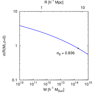
Refer to caption
(a)
Refer to caption
(b)
Figure 10: The left panel shows the variance σ𝜎\sigma at redshift z=0𝑧0z=0. Note that values of fNLsubscript𝑓NLf_{\rm NL} inside the current constraints from CMB and LSS produce no appreciable effects on σ𝜎\sigma. On the right side the 222nd and 333rd cumulant and the derivative of the latter are shown, assuming fNL=1subscript𝑓NL1f_{\rm NL}=1.

Throughout the paper we follow BSS and use an effective form of the LV mass function by replacing fLVsubscript𝑓𝐿𝑉f_{LV} with

fLVfLVfSTfPS;subscript𝑓LVsubscript𝑓LVsubscript𝑓STsubscript𝑓PSf_{\rm LV}\longrightarrow f_{\rm LV}\,\frac{f_{\rm ST}}{f_{\rm PS}}\,; (B.11)

the resulting mass function can be thought as the ST mass function corrected for non-Gaussian initial conditions.

Appendix C Comment on the fitting functions

In [103], useful fitting functions for κ3subscript𝜅3\kappa_{3} and dκ3/dMdlnσ1/dM𝑑subscript𝜅3𝑑M𝑑superscript𝜎1𝑑M\frac{d\kappa_{3}/d{\rm M}}{d\ln\sigma^{-1}/d{\rm M}} are given

κ3(1)=superscriptsubscript𝜅31absent\displaystyle\kappa_{3}^{(1)}=  0.000329(1+0.09z)b10.090.00032910.09𝑧superscriptsubscript𝑏10.09\displaystyle\,0.000329\left(1+0.09z\right)b_{1}^{-0.09}
dκ3(1)/dMdlnσ1/dM=𝑑superscriptsubscript𝜅31𝑑M𝑑superscript𝜎1𝑑Mabsent\displaystyle\frac{d\kappa_{3}^{(1)}/d{\rm M}}{d\ln\sigma^{-1}/d{\rm M}}= 0.000061(1+0.22z)b10.250.00006110.22𝑧superscriptsubscript𝑏10.25\displaystyle-0.000061\left(1+0.22z\right)b_{1}^{-0.25}

where b1=(ν21)/δc+1subscript𝑏1superscript𝜈21subscript𝛿𝑐1b_{1}=(\nu^{2}-1)/\delta_{c}+1 is the Eulerian Gaussian bias derived from the PS mass function with δc=1.42subscript𝛿𝑐1.42\delta_{c}=1.42.

As we use a combination of the ST and LV mass function with δc=1.686subscript𝛿𝑐1.686\delta_{c}=1.686, we prefer to use eq. B.10 for κ3subscript𝜅3\kappa_{3} and get dκ3/dMdlnσ1/dM𝑑subscript𝜅3𝑑M𝑑superscript𝜎1𝑑M\frac{d\kappa_{3}/d{\rm M}}{d\ln\sigma^{-1}/d{\rm M}} out of this one. We obtain

dκ3/dMdlnσ1/dM=1.056×105fNLτG2σG24.2×10101+κ2fNL21,𝑑subscript𝜅3𝑑M𝑑superscript𝜎1𝑑M1.056superscript105subscript𝑓NLsuperscriptsubscript𝜏𝐺2superscriptsubscript𝜎𝐺24.2superscript10101subscript𝜅2superscriptsubscript𝑓NL21\frac{d\kappa_{3}/d{\rm M}}{d\ln\sigma^{-1}/d{\rm M}}=\frac{1.056\times 10^{-5}f_{\rm NL}}{\frac{\tau_{G}^{2}}{\sigma_{G}^{2}}-\frac{4.2\times 10^{-10}}{1+\kappa_{2}}f_{\rm NL}^{2}-1}\,, (C.1)

where we introduced the quantity τG2superscriptsubscript𝜏𝐺2\tau_{G}^{2} that is defined as

τG2d𝐤(2π)3WMj0(kR)P0(k),superscriptsubscript𝜏𝐺2d𝐤superscript2𝜋3subscript𝑊𝑀subscript𝑗0𝑘𝑅subscript𝑃0𝑘\tau_{G}^{2}\equiv\int\frac{\,\mathrm{d}\mathbf{k}}{(2\pi)^{3}}W_{M}j_{0}(kR)P_{0}(k)\,, (C.2)

and j0(kR)subscript𝑗0𝑘𝑅j_{0}(kR) is the spherical Bessel function of order 00. κ3subscript𝜅3\kappa_{3} and dκ3/dMdlnσ1/dM𝑑subscript𝜅3𝑑M𝑑superscript𝜎1𝑑M\frac{d\kappa_{3}/d{\rm M}}{d\ln\sigma^{-1}/d{\rm M}} are plotted in fig. 10.

Appendix D Coordinate Jacobian

Since the matter density is a 333-scalar, we have

M=ρ(𝐱,z)a(z)3|gx|d3𝐱=ρ(𝐪,z)a(z)3|gq|d3𝐪,𝑀𝜌𝐱𝑧𝑎superscript𝑧3subscript𝑔𝑥superscript𝑑3𝐱𝜌𝐪𝑧𝑎superscript𝑧3subscript𝑔𝑞superscript𝑑3𝐪M=\rho(\mathbf{x},z)a(z)^{3}\sqrt{|g_{x}|}d^{3}\mathbf{x}=\rho(\mathbf{q},z)a(z)^{3}\sqrt{|g_{q}|}d^{3}\mathbf{q}\,, (D.1)

the determinant of the Eulerian metric gxsubscript𝑔𝑥g_{x} is simply |gx|=1subscript𝑔𝑥1|g_{x}|=1, but the Lagrangian space has a non-trivial metric gqsubscript𝑔𝑞g_{q} even in Newtonian theory. If we define the coordinate Jacobian

𝒥|d3𝐱d3𝐪|=|gq|,𝒥superscript𝑑3𝐱superscript𝑑3𝐪subscript𝑔𝑞{\cal J}\equiv\left|\frac{d^{3}\mathbf{x}}{d^{3}\mathbf{q}}\right|=\sqrt{|g_{q}|}\,, (D.2)

by using eq. D.1 we have to first order

𝒥1+𝚿.similar-to-or-equals𝒥1𝚿{\cal J}\simeq 1+\nabla\cdot\mathbf{\Psi}\,. (D.3)

At the initial redshift zinsubscript𝑧inz_{\rm in}, the Eulerian and Lagrangian frame are equivalent, i.e. 𝚿=0𝚿0\mathbf{\Psi}=0, and hence 𝒥=1𝒥1{\cal J}=1. If in addition we assume that the mass per volume element is conserved and the initial density was uniform, ρ(𝐪,zin)=ρ¯(zin)𝜌𝐪subscript𝑧in¯𝜌subscript𝑧in\rho(\mathbf{q},z_{\rm in})=\bar{\rho}(z_{\rm in}) in the limit zinsubscript𝑧inz_{\rm in}\to\infty, we have

M=a3(z)ρ(𝐱,z)d3𝐱=a3(zin)ρ¯(zin)d3𝐪𝑀superscript𝑎3𝑧𝜌𝐱𝑧superscript𝑑3𝐱superscript𝑎3subscript𝑧in¯𝜌subscript𝑧insuperscript𝑑3𝐪M=a^{3}(z)\rho(\mathbf{x},z)d^{3}\mathbf{x}=a^{3}(z_{\rm in})\bar{\rho}(z_{\rm in})d^{3}\mathbf{q} (D.4)

and hence

𝒥|d3𝐱d3𝐪|=a3(zin)ρ¯(zin)a3(z)ρ(𝐱,z)=ρ¯(z)ρ(𝐱,z)=[1+δE(𝐱,z)]1,𝒥superscript𝑑3𝐱superscript𝑑3𝐪superscript𝑎3subscript𝑧in¯𝜌subscript𝑧insuperscript𝑎3𝑧𝜌𝐱𝑧¯𝜌𝑧𝜌𝐱𝑧superscriptdelimited-[]1superscript𝛿E𝐱𝑧1{\cal J}\equiv\left|\frac{d^{3}\mathbf{x}}{d^{3}\mathbf{q}}\right|=\frac{a^{3}(z_{\rm in})\bar{\rho}(z_{\rm in})}{a^{3}(z)\rho(\mathbf{x},z)}=\frac{\bar{\rho}(z)}{\rho(\mathbf{x},z)}=[1+\delta^{\rm E}(\mathbf{x},z)]^{-1}\,, (D.5)

where δE(𝐱)superscript𝛿E𝐱\delta^{\rm E}(\mathbf{x}) is the Eulerian fully non-linear density contrast.

Appendix E Spherical collapse approximation: Local Eulerian biasing

The spherical collapse approximation has been used in many works (see for instance [63, 67, 44]) and we present it here with the aim of highlighting the differences respect to the more general result we derived in section 4.

The spherical collapse corresponds to the special case in which 𝚿=0𝚿0\mathbf{\Psi}=0 and the velocity field vanishes at the centre of the symmetrical collapse so that the Eulerian and Lagrangian coordinates coincide at all times, 𝐱𝐪𝐱𝐪\mathbf{x}\equiv\mathbf{q}. The results that we are going to quote all relate the density at the centre of collapse or assume a uniform density equal to that at the centre, i.e. edge effects are not considered.

Following [63] (see also [65]), the linearly growing density at the centre of the collapse relates to the non-linear density field

δlinL(𝐪)=i=0aiδ(𝐱)i=a1δ+a2δ2+,superscriptsubscript𝛿linL𝐪superscriptsubscript𝑖0subscript𝑎𝑖𝛿superscript𝐱𝑖subscript𝑎1𝛿subscript𝑎2superscript𝛿2\delta_{\rm lin}^{\rm L}(\mathbf{q})=\sum_{i=0}^{\infty}a_{i}\delta(\mathbf{x})^{i}=a_{1}\delta+a_{2}\delta^{2}+\dots\,, (E.1)

where the coefficients are

a1=1,a2=1721.formulae-sequencesubscript𝑎11subscript𝑎21721a_{1}=1,\quad a_{2}=-\frac{17}{21}\,. (E.2)

Equation E.1 is local in either Eulerian or Lagrangian coordinates since they coincide at the centre of the symmetrical collapse.

On the other hand, at the centre of collapse the auxiliary potential is simply

φG(𝐪)φG(𝐱),subscript𝜑G𝐪subscript𝜑G𝐱\varphi_{\rm G}(\mathbf{q})\equiv\varphi_{\rm G}(\mathbf{x})\,, (E.3)

where we remember that φG(𝐱)subscript𝜑G𝐱\varphi_{\rm G}(\mathbf{x}) always refer to the primordial value as it simply allows to keep track of the PNG effects in the initial density field; hence φG(𝐱)subscript𝜑G𝐱\varphi_{\rm G}(\mathbf{x}) does not evolve with time like a physical quantity do and its coordinate transformation is straightforward.

Now, using eqs. E.1 and E.3 to express δhL(𝐪)=δhL(𝐪(𝐱,τ))superscriptsubscript𝛿L𝐪superscriptsubscript𝛿L𝐪𝐱𝜏\delta_{h}^{\rm L}(\mathbf{q})=\delta_{h}^{\rm L}(\mathbf{q}(\mathbf{x},\tau)), we can solve eq. 4.3 for δhE(𝐱)superscriptsubscript𝛿E𝐱\delta_{h}^{\rm E}(\mathbf{x}). By using the same bias redefinition of eq. 4.7, the Eulerian halo overdensity finally reads

δh(𝐱)=b10Eδ+b01EφG+b20Eδ2+b11EδφG+b02EφG2.subscript𝛿𝐱superscriptsubscript𝑏10E𝛿superscriptsubscript𝑏01Esubscript𝜑Gsuperscriptsubscript𝑏20Esuperscript𝛿2superscriptsubscript𝑏11E𝛿subscript𝜑Gsuperscriptsubscript𝑏02Esubscriptsuperscript𝜑2G\begin{split}\delta_{h}(\mathbf{x})=\,&b_{10}^{\rm E}\delta+b_{01}^{\rm E}\varphi_{\rm G}+b_{20}^{\rm E}\delta^{2}+b_{11}^{\rm E}\delta\varphi_{\rm G}+b_{02}^{\rm E}\varphi^{2}_{\rm G}\,.\end{split} (E.4)

We see that the local Lagrangian biasing of eq. 3.4 is compatible with the local Eulerian model we have just obtained, despite the fact that the transformation of eq. 4.3 is inherently non local: this is true only when spherical collapse dynamics applies.

Appendix F BSS halo bispectrum

The halo bispectrum model of BSS [44] predicts

Bhhh(AL)(𝐤1,𝐤2,𝐤3)=superscriptsubscript𝐵hhhALsubscript𝐤1subscript𝐤2subscript𝐤3absent\displaystyle B_{\text{hhh}}^{(\text{A}\rightarrow\text{L})}(\mathbf{k}_{1},\mathbf{k}_{2},\mathbf{k}_{3})= b103(2P(k1)P(k2)2(𝐤1,𝐤2)+2fNLP(k1)P(k2)α(k3)α(k1)α(k2)+2cyc.)Asuperscriptsubscript𝑏103subscript2𝑃subscript𝑘1𝑃subscript𝑘2subscript2subscript𝐤1subscript𝐤22subscript𝑓NL𝑃subscript𝑘1𝑃subscript𝑘2𝛼subscript𝑘3𝛼subscript𝑘1𝛼subscript𝑘22cyc.A\displaystyle b_{10}^{3}\left(2P(k_{1})P(k_{2})\mathcal{F}_{2}(\mathbf{k}_{1},\mathbf{k}_{2})+2f_{\rm NL}\frac{P(k_{1})P(k_{2})\alpha(k_{3})}{\alpha(k_{1})\alpha(k_{2})}+2\ \text{cyc.}\right)_{\text{A}}
+\displaystyle+ b102b01(2P(k1)P(k2)(1α(k1)+1α(k2))F2(k1,k2)\displaystyle b_{10}^{2}b_{01}\left(2P(k_{1})P(k_{2})\left(\frac{1}{\alpha(k_{1})}+\frac{1}{\alpha(k_{2})}\right)F_{2}(\vec{k}_{1},\vec{k}_{2})\right.
+\displaystyle+ 2fNLP(k1)P(k2)α(k3)α(k1)α(k2)(1α(k1)+1α(k2))+2cyc.)B\displaystyle\left.2f_{\rm NL}\frac{P(k_{1})P(k_{2})\alpha(k_{3})}{\alpha(k_{1})\alpha(k_{2})}\left(\frac{1}{\alpha(k_{1})}+\frac{1}{\alpha(k_{2})}\right)+2\ \text{cyc.}\right)_{\text{B}}
+\displaystyle+ b10b012(2P(k1)P(k2)α(k1)α(k2)2(𝐤1,𝐤2)+2fNLP(k1)P(k2)α(k3)α2(k1)α2(k2)+2cyc.)Csubscript𝑏10superscriptsubscript𝑏012subscript2𝑃subscript𝑘1𝑃subscript𝑘2𝛼subscript𝑘1𝛼subscript𝑘2subscript2subscript𝐤1subscript𝐤22subscript𝑓NL𝑃subscript𝑘1𝑃subscript𝑘2𝛼subscript𝑘3superscript𝛼2subscript𝑘1superscript𝛼2subscript𝑘22cyc.C\displaystyle b_{10}b_{01}^{2}\left(2\frac{P(k_{1})P(k_{2})}{\alpha(k_{1})\alpha(k_{2})}\mathcal{F}_{2}(\mathbf{k}_{1},\mathbf{k}_{2})+2f_{\rm NL}\frac{P(k_{1})P(k_{2})\alpha(k_{3})}{\alpha^{2}(k_{1})\alpha^{2}(k_{2})}+2\ \text{cyc.}\right)_{\text{C}}
+\displaystyle+ b012b02(2P(k1)P(k2)α2(k1)α2(k2)+2cyc.)Dsuperscriptsubscript𝑏012subscript𝑏02subscript2𝑃subscript𝑘1𝑃subscript𝑘2superscript𝛼2subscript𝑘1superscript𝛼2subscript𝑘22cyc.D\displaystyle b_{01}^{2}b_{02}\left(2\frac{P(k_{1})P(k_{2})}{\alpha^{2}(k_{1})\alpha^{2}(k_{2})}+2\ \text{cyc.}\right)_{\text{D}}
+\displaystyle+ b01b10b02(2P(k1)P(k2)α(k1)α(k2)(1α(k1)+1α(k2))+2cyc.)Esubscript𝑏01subscript𝑏10subscript𝑏02subscript2𝑃subscript𝑘1𝑃subscript𝑘2𝛼subscript𝑘1𝛼subscript𝑘21𝛼subscript𝑘11𝛼subscript𝑘22cyc.E\displaystyle b_{01}b_{10}b_{02}\left(2\frac{P(k_{1})P(k_{2})}{\alpha(k_{1})\alpha(k_{2})}\left(\frac{1}{\alpha(k_{1})}+\frac{1}{\alpha(k_{2})}\right)+2\ \text{cyc.}\right)_{\text{E}}
+\displaystyle+ b102b02(2P(k1)P(k2)α(k1)α(k2)+2cyc.)Fsuperscriptsubscript𝑏102subscript𝑏02subscript2𝑃subscript𝑘1𝑃subscript𝑘2𝛼subscript𝑘1𝛼subscript𝑘22cyc.F\displaystyle b_{10}^{2}b_{02}\left(2\frac{P(k_{1})P(k_{2})}{\alpha(k_{1})\alpha(k_{2})}+2\ \text{cyc.}\right)_{\text{F}} (F.1)
+\displaystyle+ b012b11(P(k1)P(k2)α(k1)α(k2)(1α(k1)+1α(k2))+2cyc.)Gsuperscriptsubscript𝑏012subscript𝑏11subscript𝑃subscript𝑘1𝑃subscript𝑘2𝛼subscript𝑘1𝛼subscript𝑘21𝛼subscript𝑘11𝛼subscript𝑘22cyc.G\displaystyle b_{01}^{2}b_{11}\left(\frac{P(k_{1})P(k_{2})}{\alpha(k_{1})\alpha(k_{2})}\left(\frac{1}{\alpha(k_{1})}+\frac{1}{\alpha(k_{2})}\right)+2\ \text{cyc.}\right)_{\text{G}}
+\displaystyle+ b01b10b11(P(k1)P(k2)(1α2(k1)+2α(k1)α(k2)+1α2(k2))+2cyc.)Hsubscript𝑏01subscript𝑏10subscript𝑏11subscript𝑃subscript𝑘1𝑃subscript𝑘21superscript𝛼2subscript𝑘12𝛼subscript𝑘1𝛼subscript𝑘21superscript𝛼2subscript𝑘22cyc.H\displaystyle b_{01}b_{10}b_{11}\left(P(k_{1})P(k_{2})\left(\frac{1}{\alpha^{2}(k_{1})}+\frac{2}{\alpha(k_{1})\alpha(k_{2})}+\frac{1}{\alpha^{2}(k_{2})}\right)+2\ \text{cyc.}\right)_{\text{H}}
+\displaystyle+ b102b11(P(k1)P(k2)(1α(k1)+1α(k2))+2cyc.)Isuperscriptsubscript𝑏102subscript𝑏11subscript𝑃subscript𝑘1𝑃subscript𝑘21𝛼subscript𝑘11𝛼subscript𝑘22cyc.I\displaystyle b_{10}^{2}b_{11}\left(P(k_{1})P(k_{2})\left(\frac{1}{\alpha(k_{1})}+\frac{1}{\alpha(k_{2})}\right)+2\ \text{cyc.}\right)_{\text{I}}
+\displaystyle+ b012b20(2P(k1)P(k2)α(k1)α(k2)+2cyc.)Jsuperscriptsubscript𝑏012subscript𝑏20subscript2𝑃subscript𝑘1𝑃subscript𝑘2𝛼subscript𝑘1𝛼subscript𝑘22cyc.J\displaystyle b_{01}^{2}b_{20}\left(2\frac{P(k_{1})P(k_{2})}{\alpha(k_{1})\alpha(k_{2})}+2\ \text{cyc.}\right)_{\text{J}}
+\displaystyle+ b01b10b20(2P(k1)P(k2)(1α(k1)+1α(k2))+2cyc.)Ksubscript𝑏01subscript𝑏10subscript𝑏20subscript2𝑃subscript𝑘1𝑃subscript𝑘21𝛼subscript𝑘11𝛼subscript𝑘22cyc.K\displaystyle b_{01}b_{10}b_{20}\left(2P(k_{1})P(k_{2})\left(\frac{1}{\alpha(k_{1})}+\frac{1}{\alpha(k_{2})}\right)+2\ \text{cyc.}\right)_{\text{K}}
+\displaystyle+ b102b20(2P(k1)P(k2)+2cyc.)L.superscriptsubscript𝑏102subscript𝑏20subscript2𝑃subscript𝑘1𝑃subscript𝑘22cyc.L\displaystyle b_{10}^{2}b_{20}\left(2P(k_{1})P(k_{2})+2\ \text{cyc.}\right)_{\text{L}}\,.

Equation F.1 is incorporated in our prediction for the halo bispectrum but new terms appear (see eq. 5.4).

Appendix G Halo-matter bispectra

Here we consider the case of crossed bispectra between halos and matter. Potentially, weak lensing measurements will allow to cross correlate the dark matter density field with galaxies in the future. Also, these results provide additional predictions of our model that can be tested against simulations.

We start by quoting the halo-halo-matter bispectrum in presence of Gaussian initial conditions

Bhhm(𝐤1,𝐤2,𝐤3)=subscript𝐵hhmsubscript𝐤1subscript𝐤2subscript𝐤3absent\displaystyle B_{\text{hhm}}(\mathbf{k}_{1},\mathbf{k}_{2},\mathbf{k}_{3})= b102(62(𝐤1,𝐤2)P(k1)P(k2)+2cyc.)Asuperscriptsubscript𝑏102subscript6subscript2subscript𝐤1subscript𝐤2𝑃subscript𝑘1𝑃subscript𝑘22cyc.A\displaystyle b_{10}^{2}\biggl{(}6\mathcal{F}_{2}(\mathbf{k}_{1},\mathbf{k}_{2})P(k_{1})P(k_{2})+2\ \text{cyc.}\biggr{)}_{\text{A}}
+\displaystyle+ b10b20(4P(k1)P(k2)+2cyc.)Dsubscript𝑏10subscript𝑏20subscript4𝑃subscript𝑘1𝑃subscript𝑘22cyc.D\displaystyle b_{10}b_{20}\biggl{(}4P(k_{1})P(k_{2})+2\ \text{cyc.}\biggr{)}_{\text{D}} (G.1)
\displaystyle- 27b10b10L(2𝒮2(𝐤1,𝐤2)P(k1)P(k2)+2cyc.)J.27subscript𝑏10superscriptsubscript𝑏10Lsubscript2subscript𝒮2subscript𝐤1subscript𝐤2𝑃subscript𝑘1𝑃subscript𝑘22cyc.J\displaystyle\frac{2}{7}b_{10}b_{10}^{\rm L}\biggl{(}2\mathcal{S}_{2}(\mathbf{k}_{1},\mathbf{k}_{2})P(k_{1})P(k_{2})+2\ \text{cyc.}\biggr{)}_{\text{J}}\,.

Again, we recognise that it is sourced by non-linear gravitational evolution and non-linear bias, while the last term is generated by s2superscript𝑠2s^{2} in eq. 4.8.

Assuming PNG, the halo-halo-matter bispectrum888Note that the term H corrects a typo present in Eq.(5.6)5.6(5.6) of BSS. reads

Bhhm(𝐤1,𝐤2,𝐤3)=subscript𝐵hhmsubscript𝐤1subscript𝐤2subscript𝐤3absent\displaystyle B_{\text{hhm}}(\mathbf{k}_{1},\mathbf{k}_{2},\mathbf{k}_{3})= b102(62(𝐤1,𝐤2)P(k1)P(k2)+6fNLα(k3)P(k1)α(k1)P(k2)α(k2)+2cyc.)Asuperscriptsubscript𝑏102subscript6subscript2subscript𝐤1subscript𝐤2𝑃subscript𝑘1𝑃subscript𝑘26subscript𝑓NL𝛼subscript𝑘3𝑃subscript𝑘1𝛼subscript𝑘1𝑃subscript𝑘2𝛼subscript𝑘22cyc.A\displaystyle b_{10}^{2}\biggl{(}6\mathcal{F}_{2}(\mathbf{k}_{1},\mathbf{k}_{2})P(k_{1})P(k_{2})+6f_{\rm NL}\alpha(k_{3})\frac{P(k_{1})}{\alpha(k_{1})}\frac{P(k_{2})}{\alpha(k_{2})}+2\ \text{cyc.}\biggr{)}_{\text{A}}
+\displaystyle+ b01b10(42(𝐤1,𝐤2)P(k1)P(k2)(1α(k1)+1α(k2))\displaystyle b_{01}b_{10}\biggl{(}4\mathcal{F}_{2}(\mathbf{k}_{1},\mathbf{k}_{2})P(k_{1})P(k_{2})\left(\frac{1}{\alpha(k_{1})}+\frac{1}{\alpha(k_{2})}\right)
+\displaystyle+ 4fNLα(k3)P(k1)P(k2)(1α2(k1)α(k2)+1α(k1)α2(k2))+2cyc.)B\displaystyle 4f_{\rm NL}\alpha(k_{3})P(k_{1})P(k_{2})\left(\frac{1}{\alpha^{2}(k_{1})\alpha(k_{2})}+\frac{1}{\alpha(k_{1})\alpha^{2}(k_{2})}\right)+2\ \text{cyc.}\biggr{)}_{\text{B}}
+\displaystyle+ b012(22(𝐤1,𝐤2)P(k1)P(k2)α(k1)α(k2)+2fNLα(k3)P(k1)P(k2)α2(k1)α2(k2)+2cyc.)Csuperscriptsubscript𝑏012subscript2subscript2subscript𝐤1subscript𝐤2𝑃subscript𝑘1𝑃subscript𝑘2𝛼subscript𝑘1𝛼subscript𝑘22subscript𝑓NL𝛼subscript𝑘3𝑃subscript𝑘1𝑃subscript𝑘2superscript𝛼2subscript𝑘1superscript𝛼2subscript𝑘22cyc.C\displaystyle b_{01}^{2}\biggl{(}2\mathcal{F}_{2}(\mathbf{k}_{1},\mathbf{k}_{2})\frac{P(k_{1})P(k_{2})}{\alpha(k_{1})\alpha(k_{2})}+2f_{\rm NL}\alpha(k_{3})\frac{P(k_{1})P(k_{2})}{\alpha^{2}(k_{1})\alpha^{2}(k_{2})}+2\ \text{cyc.}\biggr{)}_{\text{C}}
+\displaystyle+ b10b20(4P(k1)P(k2)+2cyc.)Dsubscript𝑏10subscript𝑏20subscript4𝑃subscript𝑘1𝑃subscript𝑘22cyc.D\displaystyle b_{10}b_{20}\biggl{(}4P(k_{1})P(k_{2})+2\ \text{cyc.}\biggr{)}_{\text{D}} (G.2)
+\displaystyle+ b20b01(2P(k1)P(k2)(1α(k1)+1α(k2))+2cyc.)Esubscript𝑏20subscript𝑏01subscript2𝑃subscript𝑘1𝑃subscript𝑘21𝛼subscript𝑘11𝛼subscript𝑘22cyc.E\displaystyle b_{20}b_{01}\biggl{(}2P(k_{1})P(k_{2})\left(\frac{1}{\alpha(k_{1})}+\frac{1}{\alpha(k_{2})}\right)+2\ \text{cyc.}\biggr{)}_{\text{E}}
+\displaystyle+ b11b10(2P(k1)P(k2)(1α(k1)+1α(k2))+2cyc.)Fsubscript𝑏11subscript𝑏10subscript2𝑃subscript𝑘1𝑃subscript𝑘21𝛼subscript𝑘11𝛼subscript𝑘22cyc.F\displaystyle b_{11}b_{10}\biggl{(}2P(k_{1})P(k_{2})\left(\frac{1}{\alpha(k_{1})}+\frac{1}{\alpha(k_{2})}\right)+2\ \text{cyc.}\biggr{)}_{\text{F}}
+\displaystyle+ b11b01(P(k1)P(k2)(1α2(k1)+2α(k1)α(k2)+1α2(k2))+2cyc.)Gsubscript𝑏11subscript𝑏01subscript𝑃subscript𝑘1𝑃subscript𝑘21superscript𝛼2subscript𝑘12𝛼subscript𝑘1𝛼subscript𝑘21superscript𝛼2subscript𝑘22cyc.G\displaystyle b_{11}b_{01}\biggl{(}P(k_{1})P(k_{2})\left(\frac{1}{\alpha^{2}(k_{1})}+\frac{2}{\alpha(k_{1})\alpha(k_{2})}+\frac{1}{\alpha^{2}(k_{2})}\right)+2\ \text{cyc.}\biggr{)}_{\text{G}}
+\displaystyle+ b10b02(4P(k1)P(k2)α(k1)α(k2)+2cyc.)Hsubscript𝑏10subscript𝑏02subscript4𝑃subscript𝑘1𝑃subscript𝑘2𝛼subscript𝑘1𝛼subscript𝑘22cyc.H\displaystyle b_{10}b_{02}\biggl{(}4\frac{P(k_{1})P(k_{2})}{\alpha(k_{1})\alpha(k_{2})}+2\ \text{cyc.}\biggr{)}_{\text{H}}
+\displaystyle+ b02b01(2P(k1)P(k2)(1α2(k1)α(k2)+1α(k1)α2(k2))+2cyc.)Isubscript𝑏02subscript𝑏01subscript2𝑃subscript𝑘1𝑃subscript𝑘21superscript𝛼2subscript𝑘1𝛼subscript𝑘21𝛼subscript𝑘1superscript𝛼2subscript𝑘22cyc.I\displaystyle b_{02}b_{01}\biggl{(}2P(k_{1})P(k_{2})\left(\frac{1}{\alpha^{2}(k_{1})\alpha(k_{2})}+\frac{1}{\alpha(k_{1})\alpha^{2}(k_{2})}\right)+2\ \text{cyc.}\biggr{)}_{\text{I}}
\displaystyle- 27b10b10L(2𝒮2(𝐤1,𝐤2)P(k1)P(k2)+2cyc.)J27subscript𝑏10superscriptsubscript𝑏10Lsubscript2subscript𝒮2subscript𝐤1subscript𝐤2𝑃subscript𝑘1𝑃subscript𝑘22cyc.J\displaystyle\frac{2}{7}b_{10}b_{10}^{\rm L}\biggl{(}2\mathcal{S}_{2}(\mathbf{k}_{1},\mathbf{k}_{2})P(k_{1})P(k_{2})+2\ \text{cyc.}\biggr{)}_{\text{J}}
\displaystyle- 27b01b10L(2𝒮2(𝐤1,𝐤2)P(k1)P(k2)(1α(k1)+1α(k2))+2cyc.)K27subscript𝑏01superscriptsubscript𝑏10Lsubscript2subscript𝒮2subscript𝐤1subscript𝐤2𝑃subscript𝑘1𝑃subscript𝑘21𝛼subscript𝑘11𝛼subscript𝑘22cyc.K\displaystyle\frac{2}{7}b_{01}b_{10}^{\rm L}\biggl{(}2\mathcal{S}_{2}(\mathbf{k}_{1},\mathbf{k}_{2})P(k_{1})P(k_{2})\left(\frac{1}{\alpha(k_{1})}+\frac{1}{\alpha(k_{2})}\right)+2\ \text{cyc.}\biggr{)}_{\text{K}}
\displaystyle- b10b01L(4P(k1)P(k2)(𝒩2(𝐤1,𝐤2)α(k2)+𝒩2(𝐤2,𝐤1)α(k1))+2cyc.)Lsubscript𝑏10superscriptsubscript𝑏01Lsubscript4𝑃subscript𝑘1𝑃subscript𝑘2subscript𝒩2subscript𝐤1subscript𝐤2𝛼subscript𝑘2subscript𝒩2subscript𝐤2subscript𝐤1𝛼subscript𝑘12cyc.L\displaystyle b_{10}b_{01}^{\rm L}\biggl{(}4P(k_{1})P(k_{2})\left(\frac{\mathcal{N}_{2}(\mathbf{k}_{1},\mathbf{k}_{2})}{\alpha(k_{2})}+\frac{\mathcal{N}_{2}(\mathbf{k}_{2},\mathbf{k}_{1})}{\alpha(k_{1})}\right)+2\ \text{cyc.}\biggr{)}_{\text{L}}
\displaystyle- b01b01L(2P(k1)P(k2)(𝒩2(𝐤1,𝐤2)α(k2)+𝒩2(𝐤2,𝐤1)α(k1))(1α(k1)+1α(k2))+2cyc.)Lsubscript𝑏01superscriptsubscript𝑏01Lsubscript2𝑃subscript𝑘1𝑃subscript𝑘2subscript𝒩2subscript𝐤1subscript𝐤2𝛼subscript𝑘2subscript𝒩2subscript𝐤2subscript𝐤1𝛼subscript𝑘11𝛼subscript𝑘11𝛼subscript𝑘22cyc.L\displaystyle b_{01}b_{01}^{\rm L}\biggl{(}2P(k_{1})P(k_{2})\left(\frac{\mathcal{N}_{2}(\mathbf{k}_{1},\mathbf{k}_{2})}{\alpha(k_{2})}+\frac{\mathcal{N}_{2}(\mathbf{k}_{2},\mathbf{k}_{1})}{\alpha(k_{1})}\right)\left(\frac{1}{\alpha(k_{1})}+\frac{1}{\alpha(k_{2})}\right)+2\ \text{cyc.}\biggr{)}_{\text{L}}

The terms with label going from A to I match exactly the result of Eq.(5.6)5.6(5.6) in BSS but, as for the halo bispectrum, new terms appear. J, K are due to the tidal term s2superscript𝑠2s^{2}: schematically, they generated by s2δ(1)δ(1)delimited-⟨⟩superscript𝑠2superscript𝛿1superscript𝛿1\langle s^{2}\delta^{(1)}\delta^{(1)}\rangle, s2δ(1)φdelimited-⟨⟩superscript𝑠2superscript𝛿1𝜑\langle s^{2}\delta^{(1)}\varphi\rangle respectively. We see by comparison with eq. G.1 that J is present regardless of PNG, while K comes from the coupling between the tidal term and φ𝜑\varphi which is specifically introduced by PNG. L and M are present because of n2superscript𝑛2n^{2} and, therefore, depend on the presence of PNG. These are schematically generated by n2δ(1)δ(1)delimited-⟨⟩superscript𝑛2superscript𝛿1superscript𝛿1\langle n^{2}\delta^{(1)}\delta^{(1)}\rangle, n2δ(1)φdelimited-⟨⟩superscript𝑛2superscript𝛿1𝜑\langle n^{2}\delta^{(1)}\varphi\rangle, respectively.

Finally, for the halo-matter-matter bispectrum when Gaussian initial conditions are assumed we find

Bhmm(𝐤1,𝐤2,𝐤3)=subscript𝐵hmmsubscript𝐤1subscript𝐤2subscript𝐤3absent\displaystyle B_{\text{hmm}}(\mathbf{k}_{1},\mathbf{k}_{2},\mathbf{k}_{3})= b10(62(𝐤1,𝐤2)P(k1)P(k2)+2cyc.)Asubscript𝑏10subscript6subscript2subscript𝐤1subscript𝐤2𝑃subscript𝑘1𝑃subscript𝑘22cyc.A\displaystyle b_{10}\biggl{(}6\mathcal{F}_{2}(\mathbf{k}_{1},\mathbf{k}_{2})P(k_{1})P(k_{2})+2\ \text{cyc.}\biggr{)}_{\text{A}}
+\displaystyle+ b20(2P(k1)P(k2)+2cyc.)Csubscript𝑏20subscript2𝑃subscript𝑘1𝑃subscript𝑘22cyc.C\displaystyle b_{20}\biggl{(}2P(k_{1})P(k_{2})+2\ \text{cyc.}\biggr{)}_{\text{C}} (G.3)
\displaystyle- 27b10L(2𝒮2(𝐤1,𝐤2)P(k1)P(k2)+2cyc.)F,27superscriptsubscript𝑏10Lsubscript2subscript𝒮2subscript𝐤1subscript𝐤2𝑃subscript𝑘1𝑃subscript𝑘22cyc.F\displaystyle\frac{2}{7}b_{10}^{\rm L}\biggl{(}2\mathcal{S}_{2}(\mathbf{k}_{1},\mathbf{k}_{2})P(k_{1})P(k_{2})+2\ \text{cyc.}\biggr{)}_{\text{F}}\,,

where the same considerations for eq. G.2 apply. Then, assuming PNG, the halo-matter-matter bispectrum reads

Bhmm(𝐤1,𝐤2,𝐤3)=subscript𝐵hmmsubscript𝐤1subscript𝐤2subscript𝐤3absent\displaystyle B_{\text{hmm}}(\mathbf{k}_{1},\mathbf{k}_{2},\mathbf{k}_{3})= b10(62(𝐤1,𝐤2)P(k1)P(k2)+6fNLα(k3)P(k1)P(k2)α(k1)α(k2)+2cyc.)Asubscript𝑏10subscript6subscript2subscript𝐤1subscript𝐤2𝑃subscript𝑘1𝑃subscript𝑘26subscript𝑓NL𝛼subscript𝑘3𝑃subscript𝑘1𝑃subscript𝑘2𝛼subscript𝑘1𝛼subscript𝑘22cyc.A\displaystyle b_{10}\biggl{(}6\mathcal{F}_{2}(\mathbf{k}_{1},\mathbf{k}_{2})P(k_{1})P(k_{2})+6f_{\rm NL}\alpha(k_{3})\frac{P(k_{1})P(k_{2})}{\alpha(k_{1})\alpha(k_{2})}+2\ \text{cyc.}\biggr{)}_{\text{A}}
+\displaystyle+ b01(22(𝐤1,𝐤2)P(k1)P(k2)(1α(k1)+1α(k2))\displaystyle b_{01}\biggl{(}2\mathcal{F}_{2}(\mathbf{k}_{1},\mathbf{k}_{2})P(k_{1})P(k_{2})\left(\frac{1}{\alpha(k_{1})}+\frac{1}{\alpha(k_{2})}\right)
+\displaystyle+ 2fNLα(k3)P(k1)P(k2)(1α2(k1)α(k2)+1α(k1)α2(k2))+2cyc.)B\displaystyle 2f_{\rm NL}\alpha(k_{3})P(k_{1})P(k_{2})\left(\frac{1}{\alpha^{2}(k_{1})\alpha(k_{2})}+\frac{1}{\alpha(k_{1})\alpha^{2}(k_{2})}\right)+2\ \text{cyc.}\biggr{)}_{\text{B}}
+\displaystyle+ b20(2P(k1)P(k2)+2cyc.)Csubscript𝑏20subscript2𝑃subscript𝑘1𝑃subscript𝑘22cyc.C\displaystyle b_{20}\biggl{(}2P(k_{1})P(k_{2})+2\ \text{cyc.}\biggr{)}_{\text{C}} (G.4)
+\displaystyle+ b11(P(k1)P(k2)(1α(k1)+1α(k2))+2cyc.)Dsubscript𝑏11subscript𝑃subscript𝑘1𝑃subscript𝑘21𝛼subscript𝑘11𝛼subscript𝑘22cyc.D\displaystyle b_{11}\biggl{(}P(k_{1})P(k_{2})\left(\frac{1}{\alpha(k_{1})}+\frac{1}{\alpha(k_{2})}\right)+2\ \text{cyc.}\biggr{)}_{\text{D}}
+\displaystyle+ b02(2P(k1)P(k2)α(k1)α(k2)+2cyc.)Esubscript𝑏02subscript2𝑃subscript𝑘1𝑃subscript𝑘2𝛼subscript𝑘1𝛼subscript𝑘22cyc.E\displaystyle b_{02}\biggl{(}2\frac{P(k_{1})P(k_{2})}{\alpha(k_{1})\alpha(k_{2})}+2\ \text{cyc.}\biggr{)}_{\text{E}}
\displaystyle- 27b10L(2𝒮2(𝐤1,𝐤2)P(k1)P(k2)+2cyc.)F27superscriptsubscript𝑏10Lsubscript2subscript𝒮2subscript𝐤1subscript𝐤2𝑃subscript𝑘1𝑃subscript𝑘22cyc.F\displaystyle\frac{2}{7}b_{10}^{\rm L}\biggl{(}2\mathcal{S}_{2}(\mathbf{k}_{1},\mathbf{k}_{2})P(k_{1})P(k_{2})+2\ \text{cyc.}\biggr{)}_{\text{F}}
\displaystyle- b01L(2P(k1)P(k2)(𝒩2(𝐤1,𝐤2)α(k2)+𝒩2(𝐤2,𝐤1)α(k1))+2cyc.)G,superscriptsubscript𝑏01Lsubscript2𝑃subscript𝑘1𝑃subscript𝑘2subscript𝒩2subscript𝐤1subscript𝐤2𝛼subscript𝑘2subscript𝒩2subscript𝐤2subscript𝐤1𝛼subscript𝑘12cyc.G\displaystyle b_{01}^{\rm L}\biggl{(}2P(k_{1})P(k_{2})\left(\frac{\mathcal{N}_{2}(\mathbf{k}_{1},\mathbf{k}_{2})}{\alpha(k_{2})}+\frac{\mathcal{N}_{2}(\mathbf{k}_{2},\mathbf{k}_{1})}{\alpha(k_{1})}\right)+2\ \text{cyc.}\biggr{)}_{\text{G}}\,,

with the terms going from A to E matching exactly Eq.(5.8)5.8(5.8) of BSS. As above, new terms appear: F is due to tidal term s2superscript𝑠2s^{2} and it is generated by s2δ(1)δ(1)delimited-⟨⟩superscript𝑠2superscript𝛿1superscript𝛿1\langle s^{2}\delta^{(1)}\delta^{(1)}\rangle, regardless of the presence of PNG, while G is due to n2superscript𝑛2n^{2}, sourced by n2δ(1)δ(1)delimited-⟨⟩superscript𝑛2superscript𝛿1superscript𝛿1\langle n^{2}\delta^{(1)}\delta^{(1)}\rangle.

References

  • [1] N. Bartolo, E. Komatsu, S. Matarrese, and A. Riotto, Non-Gaussianity from inflation: Theory and observations, Phys.Rept. 402 (2004) 103–266, [astro-ph/0406398].
  • [2] D. Wands, Local non-Gaussianity from inflation, Classical and Quantum Gravity 27 (June, 2010) 124002, [arXiv:1004.0818].
  • [3] K. Koyama, Non-Gaussianity of quantum fields during inflation, Class.Quant.Grav. 27 (2010) 124001, [arXiv:1002.0600].
  • [4] M. Alvarez, T. Baldauf, J. R. Bond, N. Dalal, R. de Putter, et al., Testing Inflation with Large Scale Structure: Connecting Hopes with Reality, arXiv:1412.4671.
  • [5] C. L. Bennett, D. Larson, J. L. Weiland, N. Jarosik, G. Hinshaw, N. Odegard, K. M. Smith, R. S. Hill, B. Gold, M. Halpern, E. Komatsu, M. R. Nolta, L. Page, D. N. Spergel, E. Wollack, J. Dunkley, A. Kogut, M. Limon, S. S. Meyer, G. S. Tucker, and E. L. Wright, Nine-year Wilkinson Microwave Anisotropy Probe (WMAP) Observations: Final Maps and Results, Astrophys. J. Sup.  208 (Oct., 2013) 20, [arXiv:1212.5225].
  • [6] Planck Collaboration, P. Ade et al., Planck 2015 results. XVII. Constraints on primordial non-Gaussianity, arXiv:1502.0159.
  • [7] PRISM Collaboration, P. André et al., PRISM (Polarized Radiation Imaging and Spectroscopy Mission): An Extended White Paper, JCAP 1402 (2014) 006, [arXiv:1310.1554].
  • [8] N. Dalal, O. Dore, D. Huterer, and A. Shirokov, The imprints of primordial non-gaussianities on large-scale structure: scale dependent bias and abundance of virialized objects, Phys.Rev. D77 (2008) 123514, [arXiv:0710.4560].
  • [9] S. Matarrese and L. Verde, The effect of primordial non-Gaussianity on halo bias, Astrophys.J. 677 (2008) L77–L80, [arXiv:0801.4826].
  • [10] A. Slosar, C. Hirata, U. Seljak, S. Ho, and N. Padmanabhan, Constraints on local primordial non-Gaussianity from large scale structure, JCAP 0808 (2008) 031, [arXiv:0805.3580].
  • [11] N. Afshordi and A. J. Tolley, Primordial non-gaussianity, statistics of collapsed objects, and the Integrated Sachs-Wolfe effect, Phys.Rev. D78 (2008) 123507, [arXiv:0806.1046].
  • [12] V. Desjacques, U. Seljak, and I. Iliev, Scale-dependent bias induced by local non-Gaussianity: A comparison to N-body simulations, Mon.Not.Roy.Astron.Soc. 396 (2009) 85–96, [arXiv:0811.2748].
  • [13] V. Desjacques, D. Jeong, and F. Schmidt, Non-Gaussian Halo Bias Re-examined: Mass-dependent Amplitude from the Peak-Background Split and Thresholding, Phys. Rev.  84 (Sept., 2011) 063512, [arXiv:1105.3628].
  • [14] V. Desjacques, D. Jeong, and F. Schmidt, Accurate predictions for the scale-dependent galaxy bias from primordial non-Gaussianity, Phys. Rev.  84 (Sept., 2011) 061301, [arXiv:1105.3476].
  • [15] J.-O. Gong and S. Yokoyama, Scale-dependent bias from primordial non-Gaussianity with trispectrum, Mon. Not. Roy. Astron. Soc.  417 (Oct., 2011) L79–L82, [arXiv:1106.4404].
  • [16] D. Huterer, C. E. Cunha, and W. Fang, Calibration errors unleashed: effects on cosmological parameters and requirements for large-scale structure surveys, Mon. Not. Roy. Astron. Soc.  432 (July, 2013) 2945–2961, [arXiv:1211.1015].
  • [17] A. R. Pullen and C. M. Hirata, Systematic Effects in Large-Scale Angular Power Spectra of Photometric Quasars and Implications for Constraining Primordial Non-Gaussianity, PASP 125 (June, 2013) 705–718, [arXiv:1212.4500].
  • [18] N. Agarwal, S. Ho, A. D. Myers, H.-J. Seo, A. J. Ross, et al., Characterizing unknown systematics in large scale structure surveys, JCAP 1404 (2014) 007, [arXiv:1309.2954].
  • [19] B. Leistedt, H. V. Peiris, and N. Roth, Constraints on Primordial Non-Gaussianity from 800 000 Photometric Quasars, Phys.Rev.Lett. 113 (2014), no. 22 221301, [arXiv:1405.4315].
  • [20] A. J. Ross, W. J. Percival, A. Carnero, G.-b. Zhao, M. Manera, A. Raccanelli, E. Aubourg, D. Bizyaev, H. Brewington, J. Brinkmann, J. R. Brownstein, A. J. Cuesta, L. A. N. da Costa, D. J. Eisenstein, G. Ebelke, H. Guo, J.-C. Hamilton, M. V. Magaña, E. Malanushenko, V. Malanushenko, C. Maraston, F. Montesano, R. C. Nichol, D. Oravetz, K. Pan, F. Prada, A. G. Sánchez, L. Samushia, D. J. Schlegel, D. P. Schneider, H.-J. Seo, A. Sheldon, A. Simmons, S. Snedden, M. E. C. Swanson, D. Thomas, J. L. Tinker, R. Tojeiro, and I. Zehavi, The clustering of galaxies in the SDSS-III DR9 Baryon Oscillation Spectroscopic Survey: constraints on primordial non-Gaussianity, Mon. Not. Roy. Astron. Soc.  428 (Jan., 2013) 1116–1127, [arXiv:1208.1491].
  • [21] D. Karagiannis, T. Shanks, and N. P. Ross, Search for primordial non-Gaussianity in the quasars of SDSS-III BOSS DR9, Mon.Not.Roy.Astron.Soc. 441 (2014) 486–502, [arXiv:1310.6716].
  • [22] U. Seljak, Extracting primordial non-gaussianity without cosmic variance, Phys.Rev.Lett. 102 (2009) 021302, [arXiv:0807.1770].
  • [23] H. Gil-Marín, C. Wagner, L. Verde, R. Jimenez, and A. F. Heavens, Reducing sample variance: halo biasing, non-linearity and stochasticity, Mon. Not. Roy. Astron. Soc.  407 (Sept., 2010) 772–790, [arXiv:1003.3238].
  • [24] N. Hamaus, U. Seljak, and V. Desjacques, Optimal constraints on local primordial non-Gaussianity from the two-point statistics of large-scale structure, Phys. Rev.  84 (Oct., 2011) 083509, [arXiv:1104.2321].
  • [25] M. Biagetti, V. Desjacques, and A. Riotto, Testing multifield inflation with halo bias, Mon. Not. Roy. Astron. Soc.  429 (Feb., 2013) 1774–1780, [arXiv:1208.1616].
  • [26] L. D. Ferramacho, M. G. Santos, M. J. Jarvis, and S. Camera, Radio Galaxy populations and the multi-tracer technique: pushing the limits on primordial non-Gaussianity, Mon.Not.Roy.Astron.Soc. 442 (2014) 2511, [arXiv:1402.2290].
  • [27] D. Yamauchi, K. Takahashi, and M. Oguri, Constraining primordial non-Gaussianity via a multitracer technique with surveys by Euclid and Square Kilometre Array, Phys.Rev. D90 (2014) 083520, [arXiv:1407.5453].
  • [28] U. Seljak, N. Hamaus, and V. Desjacques, How to Suppress the Shot Noise in Galaxy Surveys, Physical Review Letters 103 (Aug., 2009) 091303, [arXiv:0904.2963].
  • [29] N. Hamaus, U. Seljak, V. Desjacques, R. E. Smith, and T. Baldauf, Minimizing the stochasticity of halos in large-scale structure surveys, Phys. Rev.  82 (Aug., 2010) 043515, [arXiv:1004.5377].
  • [30] J.-Q. Xia, M. Viel, C. Baccigalupi, G. De Zotti, S. Matarrese, and L. Verde, Primordial Non-Gaussianity and the NRAO VLA Sky Survey, Astrophys. J. Let.  717 (July, 2010) L17–L21, [arXiv:1003.3451].
  • [31] J.-Q. Xia, A. Bonaldi, C. Baccigalupi, G. De Zotti, S. Matarrese, L. Verde, and M. Viel, Constraining primordial non-Gaussianity with high-redshift probes, JCAP  8 (Aug., 2010) 13, [arXiv:1007.1969].
  • [32] T. Giannantonio, A. J. Ross, W. J. Percival, R. Crittenden, D. Bacher, et al., Improved Primordial Non-Gaussianity Constraints from Measurements of Galaxy Clustering and the Integrated Sachs-Wolfe Effect, Phys.Rev. D89 (2014) 023511, [arXiv:1303.1349].
  • [33] S. Ho, N. Agarwal, A. D. Myers, R. Lyons, A. Disbrow, et al., Sloan Digital Sky Survey III Photometric Quasar Clustering: Probing the Initial Conditions of the Universe using the Largest Volume, arXiv:1311.2597.
  • [34] T. Giannantonio and W. J. Percival, Using correlations between CMB lensing and large-scale structure to measure primordial non-Gaussianity, Mon.Not.Roy.Astron.Soc. 441 (2014) L16–L20, [arXiv:1312.5154].
  • [35] T. Giannantonio, C. Porciani, J. Carron, A. Amara, and A. Pillepich, Constraining primordial non-Gaussianity with future galaxy surveys, Mon. Not. Roy. Astron. Soc.  422 (June, 2012) 2854–2877, [arXiv:1109.0958].
  • [36] A. Raccanelli, O. Doré, D. J. Bacon, R. Maartens, M. G. Santos, et al., Probing primordial non-Gaussianity via iSW measurements with SKA continuum surveys, arXiv:1406.0010.
  • [37] S. Camera, M. G. Santos, and R. Maartens, Probing primordial non-Gaussianity with SKA galaxy redshift surveys: a fully relativistic analysis, arXiv:1409.8286.
  • [38] R. de Putter and O. Doré, Designing an Inflation Galaxy Survey: how to measure σ(fNL)1similar-to𝜎subscript𝑓NL1\sigma(f_{\rm NL})\sim 1 using scale-dependent galaxy bias, arXiv:1412.3854.
  • [39] B. Leistedt and H. V. Peiris, Exploiting the full potential of photometric quasar surveys: Optimal power spectra through blind mitigation of systematics, Mon.Not.Roy.Astron.Soc. 444 (2014) 2, [arXiv:1404.6530].
  • [40] N. Roth and C. Porciani, Can we really measure fNL from the galaxy power spectrum?, Mon. Not. Roy. Astron. Soc.  425 (Sept., 2012) L81–L85, [arXiv:1205.3165].
  • [41] Q. Mao, A. A. Berlind, C. K. McBride, R. J. Scherrer, R. Scoccimarro, et al., Constraining Primordial Non-Gaussianity with Moments of the Large Scale Density Field, Mon.Not.Roy.Astron.Soc. 443 (2014) 1402–1415, [arXiv:1404.3725].
  • [42] R. Scoccimarro, E. Sefusatti, and M. Zaldarriaga, Probing primordial non-Gaussianity with large - scale structure, Phys.Rev. D69 (2004) 103513, [astro-ph/0312286].
  • [43] E. Sefusatti and E. Komatsu, The bispectrum of galaxies from high-redshift galaxy surveys: Primordial non-Gaussianity and non-linear galaxy bias, Phys.Rev. D76 (2007) 083004, [arXiv:0705.0343].
  • [44] T. Baldauf, U. Seljak, and L. Senatore, Primordial non-Gaussianity in the Bispectrum of the Halo Density Field, JCAP 1104 (2011) 006, [arXiv:1011.1513].
  • [45] D. Jeong and E. Komatsu, Primordial Non-Gaussianity, Scale-dependent Bias, and the Bispectrum of Galaxies, Astrophys. J.  703 (Oct., 2009) 1230–1248, [arXiv:0904.0497].
  • [46] G. Tasinato, M. Tellarini, A. J. Ross, and D. Wands, Primordial non-Gaussianity in the bispectra of large-scale structure, JCAP 1403 (2014) 032, [arXiv:1310.7482].
  • [47] R. Scoccimarro, H. A. Feldman, J. N. Fry, and J. A. Frieman, The Bispectrum of IRAS redshift catalogs, Astrophys.J. 546 (2001) 652, [astro-ph/0004087].
  • [48] L. Verde, A. F. Heavens, W. J. Percival, S. Matarrese, C. M. Baugh, et al., The 2dF Galaxy Redshift Survey: The Bias of galaxies and the density of the Universe, Mon.Not.Roy.Astron.Soc. 335 (2002) 432, [astro-ph/0112161].
  • [49] Y. Jing and G. Boerner, The three-point correlation function of galaxies determined from the 2df galaxy redshift survey, Astrophys.J. 607 (2004) 140–163, [astro-ph/0311585].
  • [50] E. Gaztanaga, P. Norberg, C. Baugh, and D. Croton, Statistical analysis of galaxy surveys. 2. The 3-point galaxy correlation function measured from the 2dFGRS, Mon.Not.Roy.Astron.Soc. 364 (2005) 620–634, [astro-ph/0506249].
  • [51] F. Marín, The Large-scale Three-point Correlation Function of Sloan Digital Sky Survey Luminous Red Galaxies, Astrophys. J.  737 (Aug., 2011) 97, [arXiv:1011.4530].
  • [52] C. K. McBride, A. J. Connolly, J. P. Gardner, R. Scranton, R. Scoccimarro, A. A. Berlind, F. Marín, and D. P. Schneider, Three-point Correlation Functions of SDSS Galaxies: Constraining Galaxy-mass Bias, Astrophys. J.  739 (Oct., 2011) 85, [arXiv:1012.3462].
  • [53] WiggleZ Collaboration, F. A. Marin et al., The WiggleZ Dark Energy Survey: constraining galaxy bias and cosmic growth with 3-point correlation functions, Mon.Not.Roy.Astron.Soc. 432 (2013) 2654, [arXiv:1303.6644].
  • [54] H. Gil-Marín, J. Noreña, L. Verde, W. J. Percival, C. Wagner, et al., The power spectrum and bispectrum of SDSS DR11 BOSS galaxies I: bias and gravity, arXiv:1407.5668.
  • [55] H. Gil-Marín, L. Verde, J. Noreña, A. J. Cuesta, L. Samushia, et al., The power spectrum and bispectrum of SDSS DR11 BOSS galaxies II: cosmological interpretation, arXiv:1408.0027.
  • [56] J. N. Fry and E. Gaztanaga, Biasing and hierarchical statistics in large scale structure, Astrophys.J. 413 (1993) 447–452, [astro-ph/9302009].
  • [57] T. Baldauf, U. Seljak, V. Desjacques, and P. McDonald, Evidence for Quadratic Tidal Tensor Bias from the Halo Bispectrum, Phys.Rev. D86 (2012) 083540, [arXiv:1201.4827].
  • [58] S. Saito, T. Baldauf, Z. Vlah, U. Seljak, T. Okumura, et al., Understanding higher-order nonlocal halo bias at large scales by combining the power spectrum with the bispectrum, Phys.Rev. D90 (2014), no. 12 123522, [arXiv:1405.1447].
  • [59] K. C. Chan, R. Scoccimarro, and R. K. Sheth, Gravity and large-scale nonlocal bias, Phys. Rev.  85 (Apr., 2012) 083509, [arXiv:1201.3614].
  • [60] N. Roth and C. Porciani, Testing standard perturbation theory and the Eulerian local biasing scheme against N-body simulations, Mon. Not. Roy. Astron. Soc.  415 (July, 2011) 829–844, [arXiv:1101.1520].
  • [61] J. E. Pollack, R. E. Smith, and C. Porciani, A new method to measure galaxy bias, arXiv:1309.0504.
  • [62] P. McDonald and A. Roy, Clustering of dark matter tracers: generalizing bias for the coming era of precision LSS, JCAP  8 (Aug., 2009) 20, [arXiv:0902.0991].
  • [63] H. Mo and S. D. White, An Analytic model for the spatial clustering of dark matter halos, Mon.Not.Roy.Astron.Soc. 282 (1996) 347, [astro-ph/9512127].
  • [64] R. K. Sheth, K. C. Chan, and R. Scoccimarro, Nonlocal Lagrangian bias, Phys. Rev.  87 (Apr., 2013) 083002, [arXiv:1207.7117].
  • [65] T. Matsubara, Nonlinear perturbation theory integrated with nonlocal bias, redshift-space distortions, and primordial non-Gaussianity, Phys. Rev.  83 (Apr., 2011) 083518, [arXiv:1102.4619].
  • [66] P. Catelan, C. Porciani, and M. Kamionkowski, Two ways of biasing galaxy formation, Mon.Not.Roy.Astron.Soc. 318 (2000) 39, [astro-ph/0005544].
  • [67] T. Giannantonio and C. Porciani, Structure formation from non-Gaussian initial conditions: multivariate biasing, statistics, and comparison with N-body simulations, Phys.Rev. D81 (2010) 063530, [arXiv:0911.0017].
  • [68] E. Sefusatti, M. Crocce, and V. Desjacques, The matter bispectrum in N-body simulations with non-Gaussian initial conditions, Mon. Not. Roy. Astron. Soc.  406 (Aug., 2010) 1014–1028, [arXiv:1003.0007].
  • [69] R. Scoccimarro, L. Hui, M. Manera, and K. C. Chan, Large-scale bias and efficient generation of initial conditions for nonlocal primordial non-Gaussianity, Phys. Rev.  85 (Apr., 2012) 083002, [arXiv:1108.5512].
  • [70] S. Yokoyama, T. Matsubara, and A. Taruya, Halo/galaxy bispectrum with primordial non-Gaussianity from integrated perturbation theory, Phys.Rev. D89 (2014), no. 4 043524, [arXiv:1310.4925].
  • [71] A. Gangui, F. Lucchin, S. Matarrese, and S. Mollerach, The Three point correlation function of the cosmic microwave background in inflationary models, Astrophys.J. 430 (1994) 447–457, [astro-ph/9312033].
  • [72] L. Verde, L.-M. Wang, A. Heavens, and M. Kamionkowski, Large scale structure, the cosmic microwave background, and primordial non-gaussianity, Mon.Not.Roy.Astron.Soc. 313 (2000) L141–L147, [astro-ph/9906301].
  • [73] E. Komatsu and D. N. Spergel, Acoustic signatures in the primary microwave background bispectrum, Phys.Rev. D63 (2001) 063002, [astro-ph/0005036].
  • [74] N. Bartolo, S. Matarrese, O. Pantano, and A. Riotto, Second-order matter perturbations in a ΛΛ\LambdaCDM cosmology and non-Gaussianity, Classical and Quantum Gravity 27 (June, 2010) 124009, [arXiv:1002.3759].
  • [75] M. Bruni, J. C. Hidalgo, N. Meures, and D. Wands, Non-Gaussian Initial Conditions in ΛCDM: Newtonian, Relativistic, and Primordial Contributions, Astrophys.J. 785 (2014) 2, [arXiv:1307.1478].
  • [76] M. Bruni, J. C. Hidalgo, and D. Wands, Einstein’s signature in cosmological large-scale structure, Astrophys.J. 794 (2014), no. 1 L11, [arXiv:1405.7006].
  • [77] http://camb.info/.
  • [78] P. Ade et al., Planck 2013 Results. XXIV. Constraints on primordial non-Gaussianity, Astron.Astrophys. 571 (2014) A24, [arXiv:1303.5084].
  • [79] F. Bernardeau, S. Colombi, E. Gaztanaga, and R. Scoccimarro, Large scale structure of the universe and cosmological perturbation theory, Phys.Rept. 367 (2002) 1–248, [astro-ph/0112551].
  • [80] D. Bertacca, N. Bartolo, M. Bruni, K. Koyama, R. Maartens, et al., Galaxy bias and gauges at second order in General Relativity, arXiv:1501.0316.
  • [81] M. Schmittfull, T. Baldauf, and U. Seljak, Near optimal bispectrum estimators for large-scale structure, Phys.Rev. D91 (2015), no. 4 043530, [arXiv:1411.6595].
  • [82] P. Peebles, The Large-scale Structure of the Universe. Princeton series in physics. Princeton University Press, 1980.
  • [83] N. Kaiser, On the Spatial correlations of Abell clusters, Astrophys.J. 284 (1984) L9–L12.
  • [84] D. Baumann, S. Ferraro, D. Green, and K. M. Smith, Stochastic bias from non-Gaussian initial conditions, JCAP  5 (May, 2013) 1, [arXiv:1209.2173].
  • [85] R. Scoccimarro, R. K. Sheth, L. Hui, and B. Jain, How many galaxies fit in a halo? Constraints on galaxy formation efficiency from spatial clustering, Astrophys.J. 546 (2001) 20–34, [astro-ph/0006319].
  • [86] P. Catelan, F. Lucchin, S. Matarrese, and C. Porciani, The bias field of dark matter halos, Mon.Not.Roy.Astron.Soc. 297 (1998) 692–712, [astro-ph/9708067].
  • [87] R. Scoccimarro and H. Couchman, A fitting formula for the nonlinear evolution of the bispectrum, Mon.Not.Roy.Astron.Soc. 325 (2001) 1312, [astro-ph/0009427].
  • [88] H. Gil-Marín, C. Wagner, F. Fragkoudi, R. Jimenez, and L. Verde, An improved fitting formula for the dark matter bispectrum, JCAP  2 (Feb., 2012) 47, [arXiv:1111.4477].
  • [89] E. Sefusatti, M. Crocce, and V. Desjacques, The halo bispectrum in N-body simulations with non-Gaussian initial conditions, Mon. Not. Roy. Astron. Soc.  425 (Oct., 2012) 2903–2930, [arXiv:1111.6966].
  • [90] R. Laureijs, J. Amiaux, S. Arduini, J. . Auguères, J. Brinchmann, R. Cole, M. Cropper, C. Dabin, L. Duvet, A. Ealet, and et al., Euclid Definition Study Report, ArXiv e-prints (Oct., 2011) [arXiv:1110.3193].
  • [91] W. H. Press and P. Schechter, Formation of Galaxies and Clusters of Galaxies by Self-Similar Gravitational Condensation, Astrophys. J.  187 (Feb., 1974) 425–438.
  • [92] J. M. Bardeen, J. R. Bond, N. Kaiser, and A. S. Szalay, The statistics of peaks of Gaussian random fields, Astrophys. J.  304 (May, 1986) 15–61.
  • [93] J. R. Bond, S. Cole, G. Efstathiou, and N. Kaiser, Excursion set mass functions for hierarchical Gaussian fluctuations, Astrophys. J.  379 (Oct., 1991) 440–460.
  • [94] A. R. Zentner, The Excursion Set Theory of Halo Mass Functions, Halo Clustering, and Halo Growth, Int.J.Mod.Phys. D16 (2007) 763–816, [astro-ph/0611454].
  • [95] T. Kitayama and Y. Suto, Semianalytical predictions for statistical properties of x-ray clusters of galaxies in cold dark matter universes, Astrophys.J. 469 (1996) 480, [astro-ph/9604141].
  • [96] V. R. Eke, S. Cole, and C. S. Frenk, Using the evolution of clusters to constrain Omega, Mon.Not.Roy.Astron.Soc. 282 (1996) 263–280, [astro-ph/9601088].
  • [97] R. K. Sheth and G. Tormen, Large-scale bias and the peak background split, Mon. Not. Roy. Astron. Soc.  308 (Sept., 1999) 119–126, [astro-ph/9901122].
  • [98] R. K. Sheth, H. J. Mo, and G. Tormen, Ellipsoidal collapse and an improved model for the number and spatial distribution of dark matter haloes, Mon. Not. Roy. Astron. Soc.  323 (May, 2001) 1–12, [astro-ph/9907024].
  • [99] R. K. Sheth and G. Tormen, An excursion set model of hierarchical clustering: ellipsoidal collapse and the moving barrier, Mon. Not. Roy. Astron. Soc.  329 (Jan., 2002) 61–75, [astro-ph/0105113].
  • [100] M. LoVerde, A. Miller, S. Shandera, and L. Verde, Effects of Scale-Dependent Non-Gaussianity on Cosmological Structures, JCAP 0804 (2008) 014, [arXiv:0711.4126].
  • [101] M. LoVerde and K. M. Smith, The non-Gaussian halo mass function with fNL, gNL and τ𝜏\tauNL, JCAP  8 (Aug., 2011) 3, [arXiv:1102.1439].
  • [102] T. Suyama and M. Yamaguchi, Non-Gaussianity in the modulated reheating scenario, Phys.Rev. D77 (2008) 023505, [arXiv:0709.2545].
  • [103] K. M. Smith, S. Ferraro, and M. LoVerde, Halo clustering and gNL-type primordial non-gaussianity, JCAP 1203 (2012) 032, [arXiv:1106.0503].