Planck 2015 results. XIV. Dark energy and modified gravity

We study the implications of Planck data for models of dark energy (DE) and modified gravity (MG), beyond the standard cosmological constant scenario. We start with cases where the DE only directly affects the background evolution, considering Taylor expansions of the equation of state $w(a)$, as well as principal component analysis and parameterizations related to the potential of a minimally coupled DE scalar field. When estimating the density of DE at early times, we significantly improve present constraints and find that it has to be below $\approx 2\thinspace\%$ (at $95\%$ confidence) of the critical density even when forced to play a role for $z<50$ only. We then move to general parameterizations of the DE or MG perturbations that encompass both effective field theories and the phenomenology of gravitational potentials in MG models. Lastly, we test a range of specific models, such as k-essence, $f(R)$ theories and coupled DE. In addition to the latest Planck data, for our main analyses we use background constraints from baryonic acoustic oscillations, type-Ia supernovae and local measurements of the Hubble constant. We further show the impact of measurements of the cosmological perturbations, such as redshift-space distortions and weak gravitational lensing. These additional probes are important tools for testing MG models and for breaking degeneracies that are still present in the combination of Planck and background data sets.

All results that include only background parameterizations (expansion of the equation of state, early DE, general potentials in minimally-coupled scalar fields or principal component analysis) are in agreement with $\rm{\Lambda CDM}$. When testing models that also change perturbations (even when the background is fixed to $\rm{\Lambda CDM}$), some tensions appear in a few scenarios: the maximum one found is $\sim 2\sigma$ for Planck TT+lowP when parameterizing observables related to the gravitational potentials with a chosen time dependence; the tension increases to at most $3\sigma$ when external data sets are included. It however disappears when including CMB lensing.

1 Introduction

The cosmic microwave background (CMB) is a key probe of our cosmological model (Planck Collaboration XIII 2015), providing information on the primordial Universe and its physics, including inflationary models (Planck Collaboration XX 2015) and constraints on primordial non-Gaussianities (Planck Collaboration XVII 2015). In this paper we use the 2015 data release from Planck (Planck Collaboration I 2015) to perform a systematic analysis of a large set of dark energy and modified gravity theories.

Observations have long shown that only a small fraction of the total energy density in the Universe (around 5 %) is in the form of baryonic matter, with the dark matter needed for structure formation accounting for about another 26 %. In one scenario the dominant component, generically referred to as dark energy (hereafter DE), brings the total close to the critical density and is responsible for the recent phase of accelerated expansion. In another scenario the accelerated expansion arises, partly or fully, due to a modification of gravity on cosmological scales. Elucidating the nature of this DE and testing General Relativity (GR) on cosmological scales are major challenges for contemporary cosmology, both on the theoretical and experimental sides (e.g., LSST Science Collaboration et al. 2009; Amendola et al. 2012a; Clifton et al. 2012; Joyce et al. 2014; Huterer et al. 2015).

In preparation for future experimental investigations of DE and modified gravity (hereafter MG), it is important to determine what we already know about these models at different epochs in redshift and different length scales. CMB anisotropies fix the cosmology at early times, while additional cosmological data sets further constrain on how DE or MG evolve at lower redshifts. The aim of this paper is to investigate models for dark energy and modified gravity using Planck data in combination with other data sets.

The simplest model for DE is a cosmological constant, $\Lambda$, first introduced by Einstein (1917) in order to keep the Universe static, but soon dismissed when the Universe was found to be expanding (Lemaître 1927; Hubble 1929). This constant has been reintroduced several times over the years in attempts to explain several astrophysical phenomena, including most recently the flat spatial geometry implied by the CMB and supernova observations of a recent phase of accelerated expansion (Riess et al. 1998; Perlmutter et al. 1999). A cosmological constant is described by a single parameter, the inclusion of which brings the model ($\Lambda$CDM) into excellent agreement with the data. $\Lambda$CDM still represents a good fit to a wide range of observations, more than 20 years after it was introduced. Nonetheless, theoretical estimates for the vacuum density are many orders of magnitude larger than its observed value. In addition, $\Omega_{\Lambda}$ and $\Omega_{\rm m}$ are of the same order of magnitude only at present, which marks our epoch as a special time in the evolution of the Universe (the “coincidence problem”). This lack of a clear theoretical understanding has motivated the development of a wide variety of alternative models. Those models which are close to $\Lambda$CDM are in broad agreement with current constraints on the background cosmology, but the perturbations may still evolve differently, and hence it is important to test their predictions against CMB data.

There are at least three difficulties we had to face within this paper. First, there appears to be a vast array of possibilities in the literature and no agreement yet in the scientific community on a comprehensive framework for discussing the landscape of models. A second complication is that robust constraints on DE come from a combination of different data sets working in concert. Hence we have to be careful in the choice of the data sets so that we do not find apparent hints for non-standard models that are in fact due to systematic errors. A third area of concern is the fact that numerical codes available at present for DE and MG are not as well tested in these scenarios as for $\rm{\Lambda CDM}$, especially given the accuracy reached by the data. Furthermore, in some cases, we need to rely on stability routines that deserve further investigation to assure that they are not excluding more models than required.

In order to navigate the range of modelling possibilities, we adopt the following three-part approach.

1. Background parameterizations. Here we consider only parameterizations of background-level cosmological quantities. Perturbations are always included, but their evolution depends only on the background. This set includes models involving expansions, parameterizations or principal component analyses of the equation of state $w\equiv p/\rho$ of a DE fluid with pressure $p$ and energy density $\rho$. Early DE also belongs to this class.

2. Perturbation parameterizations. Here the perturbations themselves are parameterized or modified explicitly, not only as a consequence of a change in background quantities. There are two main branches we consider: firstly, effective field theory for DE (EFT, e.g.  Gubitosi et al. 2013), which has a clear theoretical motivation, since it includes all theories derived when accounting for all symmetry operators in the Lagrangian, written in unitary gauge, i.e. in terms of metric perturbations only. This is a very general classification that has the advantage of providing a broad overview of (at least) all universally coupled DE models. However, a clear disadvantage is that the number of free parameters is large and the constraints are consequently weak. Moreover, in currently available numerical codes one needs to rely on stability routines which are not fully tested and may discard more models than necessary.

   As a complementary approach, we include a more phenomenological class of models obtained by directly parameterizing two independent functions of the gravitational potentials. This approach can in principle probe all degrees of freedom at the background and perturbation level (e.g. Kunz 2012) and is easier to handle in numerical codes. While the connection to physical models is less obvious here than in EFT, this approach allows us to gain a more intuitive understanding of the general constraining power of the data.

3. Examples of particular models. Here we focus on a selection of theories that have already been discussed in the literature and are better understood theoretically; these can partly be considered as applications of previous cases for which the CMB constraints are more informative, because there is less freedom in any particular theory than in a more general one.

The CMB is the cleanest probe of large scales, which are of particular interest for modifications to gravity. We will investigate the constraints coming from Planck data in combination with other data sets, addressing strengths and potential weaknesses of different analyses. Before describing in detail the models and data sets that correspond to our requirements, in Sect. 2 we first address the main question that motivates our paper, discussing why CMB is relevant for DE. We then present the specific model parameterizations in Sect. 3. The choice of data sets is discussed in detail in Sec. 4 before we present results in Sect. 5 and discuss conclusions in Sect. 6.

2 Why is the CMB relevant for dark energy?

The CMB anisotropies are largely generated at the last-scattering epoch, and hence can be used to pin down the theory at early times. In fact many forecasts of future DE or MG experiments are for new data plus constraints from Planck. However, there are also several effects that DE and MG models can have on the CMB, some of which are to:

1. change the expansion history and hence distance to the last scattering surface, with a shift in the peaks, sometimes referred to as a geometrical projection effect (Hu & White 1996);

2. cause the decay of gravitational potentials at late times, affecting the low-multipole CMB anisotropies through the integrated Sachs-Wolfe (or ISW) effect (Sachs & Wolfe 1967; Kofman & Starobinskii 1985);

3. enhance the cross-correlation between the CMB and large-scale structure, through the ISW effect (Giannantonio et al. 2008);

4. change the lensing potential, through additional DE perturbations or modifications of GR (Acquaviva & Baccigalupi 2006; Carbone et al. 2013);

5. change the growth of structure (Peebles 1984; Barrow & Saich 1993) leading to a mismatch between the CMB-inferred amplitude of the fluctuations $A_{\rm s}$ and late-time measurements of $\sigma_{8}$ (Kunz et al. 2004; Baldi & Pettorino 2011);

6. impact small scales, modifying the damping tail in $C_{\ell}^{TT}$, giving a measurement of the abundance of DE at different redshifts (Calabrese et al. 2011; Reichardt et al. 2012);

7. affect the ratio between odd and even peaks if modifications of gravity treat baryons and cold dark matter differently (Amendola et al. 2012b);

8. modify the lensing $B$-mode contribution, through changes in the lensing potential (Amendola et al. 2014);

9. modify the primordial $B$-mode amplitude and scale dependence, by changing the sound speed of gravitational waves (Antolini et al. 2013; Amendola et al. 2014; Raveri et al. 2014).

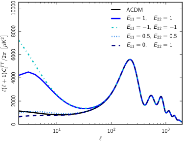
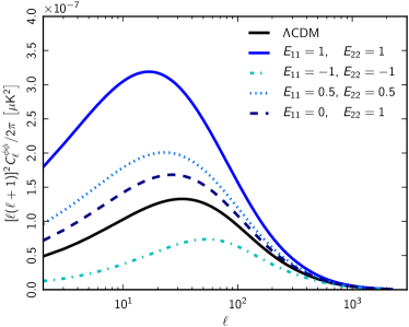
In this paper we restrict our analysis to scalar perturbations. The dominant effects on the temperature power spectrum are due to lensing and the ISW effect, as can be seen in Fig. 1, which shows typical power spectra of temperature anisotropies and lensing potential for modified gravity models. Different curves correspond to different choices of the $\mu$ and $\eta$ functions, which change the relation between the metric potentials and the sources, as well as introducing a gravitational slip; we will define these functions in Sect. 3.2.2, Eq. (4) and Eq. (6), respectively. Spectra are obtained using a scale-independent evolution for both $\mu$ and $\eta$. The two parameters in the figure then determine the change in amplitude of $\mu$ and $\eta$ with respect to the $\Lambda$CDM case, in which $E_{11}=E_{22}=0$ and $\mu=\eta=1$.

Figure 1: Typical effects of modified gravity on theoretical CMB temperature (top panel) and lensing potential (bottom panel) power spectra. An increase (or decrease) of $E_{22}$ with respect to zero introduces a gravitational slip, higher at present, when $\Omega_{\mathrm{de}}$ is higher (see Eq. (4) and Eq. (6)); this in turns changes the Weyl potential and leads to a higher (or lower) lensing potential. On the other hand, whenever $E_{11}$ and $E_{22}$ are different from zero (quite independently of their sign) $\mu$ and $\eta$ change in time: as the dynamics in the gravitational potential is increased, this leads to an enhancement in the ISW effect. Note also that even when the temperature spectrum is very close to $\rm{\Lambda CDM}$ (as for $E_{11}=E_{22}=0.5$) the lensing potential is still different with respect to $\rm{\Lambda CDM}$, shown in black.

3 Models and parameterizations

We now provide an overview of the models addressed in this paper. Details on the specific parameterizations will be discussed in Sect. 5, where we also present the results for each specific method.

We start by noticing that one can generally follow two different approaches: (1) given a theoretical set up, one can specify the action (or Lagrangian) of the theory and derive background and perturbation equations in that framework; or (2) more phenomenologically, one can construct functions that map closely onto cosmological observables, probing the geometry of spacetime and the growth of perturbations. Assuming spatial flatness for simplicity, the geometry is given by the expansion rate $H$ and perturbations to the metric. If we consider only scalar-type components the metric perturbations can be written in terms of the gravitational potentials $\Phi$ and $\Psi$ (or equivalently by any two independent combinations of these potentials). Cosmological observations thus constrain one “background” function of time $H(a)$ and two “perturbation” functions of scale and time $\Phi(k,a)$ and $\Psi(k,a)$ (e.g., Kunz 2012). These functions fix the metric, and thus the Einstein tensor $G_{\mu\nu}$. Einstein’s equations link this tensor to the energy-momentum tensor $T_{\mu\nu}$, which in turn can be related to DE or MG properties.

Throughout this paper we will adopt the metric given by the line element

$$ds^{2}=a^{2}\left[-(1+2\Psi)d\tau^{2}+(1-2\Phi)dx^{2}\right]\thinspace.$$ (1)

The gauge invariant potentials $\Phi$ and $\Psi$ are related to the Bardeen (1980) potentials $\Phi_{\rm{A}}$ and $\Phi_{H}$ and to the Kodama & Sasaki (1984) potentials ${\Psi_{\rm{KS}}}$ and ${\Phi_{\rm{KS}}}$ in the following way: $\Psi=\Phi_{\rm{A}}=\Psi_{\rm{KS}}$ and $\Phi=-\Phi_{\rm{H}}=-\Phi_{\rm{KS}}$. Throughout the paper we use a metric signature $(-,+++)$ and follow the notation of Ma & Bertschinger (1995); the speed of light is set to $c=1$, except where explicitly stated otherwise.

We define the equation of state $\bar{p}(a)=w(a)\bar{\rho}(a)$, where $\bar{p}$ and $\bar{\rho}$ are the average pressure and energy density. The sound speed $c_{\rm{s}}$ is defined in the fluid rest frame in terms of pressure and density perturbations as $\delta p(k,a)=c_{\rm{s}}^{2}(k,a)\delta\rho(k,a)$. The anisotropic stress $\sigma(k,a)$ (equivalent to $\pi_{\rm T}$ in the notation of Kodama & Sasaki 1984) is the scalar part of the off-diagonal space-space stress energy tensor perturbation. The set of functions $\{H,\Phi,\Psi\}$ describing the metric is formally equivalent to the set of functions $\{w,c_{\rm{s}}^{2},\sigma\}$ (Ballesteros et al. 2012).

Specific theories typically cover only subsets of this function space and thus make specific predictions for their form. In the following sections we will discuss the particular theories that we consider in this paper.

3.1 Background parameterizations

The first main ‘category’ of theories we describe includes parameterizations of background quantities. Even when we are only interested in constraints on background parameters, we are implicitly assuming a prescription for Dark Energy fluctuations. The conventional approach, that we adopt also here, is to choose a minimally-coupled scalar field model (Wetterich 1988; Ratra & Peebles 1988), also known as quintessence, which corresponds to the choice of a rest-frame sound speed $c_{\rm s}^{2}=1$ (i.e., equal to the speed of light) and $\sigma=0$ (no scalar anisotropic stress). In this case the relativistic sound speed suppresses the dark energy perturbations on sub-horizon scales, preventing it from contributing significantly to clustering.

Background parameterizations discussed in this paper include:

• ($w_{0}$, $w_{a}$) Taylor expansion at first order (and potentially higher orders);

• Principal Component Analysis of $w(a)$ (Huterer & Starkman 2003), that allows to estimate constraints on $w$ in independent redshift bins;

• general parameterization of any minimally coupled scalar field in terms of three parameters $\epsilon_{s}$, $\zeta_{s}$, $\epsilon_{\infty}$. This is a novel way to describe minimally coupled scalar field models without explicitly specifying the form of the potential (Huang et al. 2011);

• Dark Energy density as a function of $z$ (including parameterizations such as early Dark Energy).

The specific implementation for each of them is discussed in Sect. 5.1 together with corresponding results. We will conclude the background investigation by describing, in Sect. 5.1.6, a compressed Gaussian likelihood that captures most of the constraining power of the Planck data applied to smooth Dark Energy or curved models (following Mukherjee et al. 2008). The compressed likelihood is useful for example to include more easily the Planck CMB data in Fisher-forecasts for future large-scale structure surveys.

3.2 Perturbation parameterizations

Modified gravity models (in which gravity is modified with respect to GR) in general affect both the background and the perturbation equations. In this subsection we go beyond background parameterizations and identify two different approaches to constrain MG models, one more theoretically motivated and a second more phenomenological one. We will not embark on a full-scale survey of DE and MG models here, but refer the reader to e.g. Amendola et al. (2013) for more details.

3.2.1 Modified gravity and effective field theory

The first approach starts from a Lagrangian, derived from an effective field theory (EFT) expansion (Cheung et al. 2008), discussed in Creminelli et al. (2009) and Gubitosi et al. (2013) in the context of DE. Specifically, EFT describes the space of (universally coupled) scalar field theories, with a Lagrangian written in unitary gauge that preserves isotropy and homogeneity at the background level, assumes the weak equivalence principle, and has only one extra dynamical field besides the matter fields conventionally considered in cosmology. The action reads:

$$S = \int d^{4}x\sqrt{-g}\left\{\frac{m_{0}^{2}}{2}\left[1+\Omega(\tau)\right]R+\Lambda(\tau)-a^{2}c(\tau)\delta g^{00}\right.$$ (2)

$$\left.+\ \frac{M_{2}^{4}(\tau)}{2}\left(a^{2}\delta g^{00}\right)^{2}-\bar{M}_{1}^{3}(\tau){2}a^{2}\delta g^{00}\delta{K}^{\mu}_{\mu}\right.$$

$$\left.-\ \frac{\bar{M}_{2}^{2}(\tau)}{2}\left(\delta K^{\mu}_{\mu}\right)^{2}-\frac{\bar{M}_{3}^{2}(\tau)}{2}\delta K^{\mu}_{\nu}\delta K^{\nu}_{\mu}+\frac{a^{2}\hat{M}^{2}(\tau)}{2}\delta g^{00}\delta R^{(3)}\right.$$

$$\left.+\ m_{2}^{2}(\tau)\left(g^{\mu\nu}+n^{\mu}n^{\nu}\right)\partial_{\mu}\left(a^{2}g^{00}\right)\partial_{\nu}\left(a^{2}g^{00}\right)\vphantom{\frac{m_{0}^{2}}{2}}\right\}$$

$$+\ S_{\rm{m}}\big{[}\chi_{i},g_{\mu\nu}\big{]}.$$

Here $R$ is the Ricci scalar, $\delta R^{(3)}$ is its spatial perturbation, ${K}^{\mu}_{\nu}$ is the extrinsic curvature, and $m_{0}$ is the bare (reduced) Planck mass. The matter part of the action, $S_{\rm{m}}$, includes all fluid components except dark energy, i.e., baryons, cold dark matter, radiation, and neutrinos. The action in Eq. (2) depends on nine time-dependent functions (Bloomfield et al. 2013), here $\{\Omega,c,\Lambda,\bar{M}_{1}^{3},\bar{M}_{2}^{4},\bar{M}_{3}^{2},M_{2}^{4},\hat{M}^{2},m_{2}^{2}\}$, whose choice specifies the theory. In this way, EFT provides a direct link to any scalar field theory. A particular subset of EFT theories are the Horndeski (1974) models, which include (almost) all stable scalar-tensor theories, universally coupled to gravity, with second-order equations of motion in the fields and depend on five functions of time (Gleyzes et al. 2013; Bellini & Sawicki 2014; Piazza et al. 2014).

Although the EFT approach has the advantage of being very versatile, in practice it is necessary to choose suitable parameterizations for the free functions listed above, in order to compare the action with the data. We will describe our specific choices, together with results for each of them, in Sect. 5.2.

3.2.2 MG and phenomenological parameterizations

The second approach adopted in this paper to test MG is more phenomenological and starts from the consideration that cosmological observations probe quantities related to the metric perturbations, in addition to the expansion rate. Given the line element of Eq. (1), the metric perturbations are determined by the two potentials $\Phi$ and $\Psi$, so that we can model all observationally relevant degrees of freedom by parameterizing these two potentials (or, equivalently, two independent combinations of them) as functions of time and scale. Since a non-vanishing anisotropic stress (proportional to $\Phi-\Psi$) is a generic signature of modifications of GR (Mukhanov et al. 1992; Saltas et al. 2014), the parameterized potentials will correspond to predictions of MG models.

Various parameterizations have been considered in the literature. Some of the more popular (in longitudinal gauge) are:

1. $Q(a,\@vec{k})$, which modifies the relativistic Poisson equation through extra DE clustering according to

   $$-k^{2}\Phi\equiv 4\pi Ga^{2}Q(a,\@vec{k})\rho\Delta,$$ (3)

   where $\Delta$ is the comoving density perturbation;

2. $\mu(a,\@vec{k})$ (sometimes also called $Y(a,\@vec{k})$), which modifies the equivalent equation for $\Psi$ rather than $\Phi$:

   $$-k^{2}\Psi\equiv 4\pi Ga^{2}\mu(a,\@vec{k})\rho\Delta;$$ (4)

3. $\Sigma(a,\@vec{k})$, which modifies lensing (with the lensing/Weyl potential being $\Phi+\Psi$), such that

   $$-k^{2}(\Phi+\Psi)\equiv 8\pi Ga^{2}\Sigma(a,\@vec{k})\rho\Delta;$$ (5)

4. $\eta(a,\@vec{k})$, which reflects the presence of a non-zero anisotropic stress, the difference between $\Phi$ and $\Psi$ being equivalently written as a deviation of the ratio

   $$\eta(a,\@vec{k})\equiv\Phi/\Psi.$$ (6)

In the equations above, $\rho\Delta=\rho_{\rm m}\Delta_{\rm m}+\rho_{\rm r}\Delta_{\rm r}$ so that the parameters $Q$, $\mu$, or $\Sigma$ quantify the deviation of the gravitational potentials from the value expected in GR due to perturbations of matter and relativistic particles. At low redshifts, where most DE models become relevant, we can neglect the relativistic contribution. The same is true for $\eta$, where we can neglect the contribution of relativistic particles to the anisotropic stress at late times.

The four functions above are certainly not independent. It is sufficient to choose two independent functions of time and scale to describe all modifications with respect to General Relativity (e.g. Zhang et al. 2007; Amendola et al. 2008b). Popular choices include: $(\mu,\eta)$, which have a simple functional form for many theories; $(\mu,\Sigma)$, which is more closely related to what we actually observe, given that CMB lensing, weak galaxy lensing and the ISW effect measure a projection or derivative of the Weyl potential $\Phi+\Psi$. Furthermore, redshift space distortions constrain the velocity field, which is linked to $\Psi$ through the Euler equation of motion.

All four quantities, $Q$, $\mu$, $\Sigma$, and $\eta$, are free functions of time and scale. Their parameterization in terms of the scale factor $a$ and momentum $\@vec{k}$ will be specified in Section 5.2.2, together with results obtained by confronting this class of models with data.

3.3 Examples of particular models

The last approach is to consider particular models. Even though these are in principle included in the case described in Sect. 3.2.1, it is nevertheless still useful to highlight some well known examples of specific interest, which we list below.

• Minimally-coupled models beyond simple quintessence. Specifically, we consider “k-essence” models, which are defined by an arbitrary sound speed $c_{\rm s}^{2}$ in addition to a free equation of state parameter $w$ (Armendariz-Picon et al. 2000).

• An example of a generalized scalar field model (Deffayet et al. 2010) and of Lorentz-violating massive gravity (Dubovsky 2004; Rubakov & Tinyakov 2008), both in the ‘equation of state’ formalism of Battye & Pearson (2012).

• Universal “fifth forces.” We will show results for $f(R)$ theories (Wetterich 1995a; Capozziello 2002; Amendola et al. 2007; De Felice & Tsujikawa 2010), which form a subset of all models contained in the EFT approach.

• Non-universal fifth forces. We will illustrate results for coupled DE models (Amendola 2000), in which dark matter particles feel a force mediated by the DE scalar field.

All these particular models are based on specific actions, ensuring full internal consistency. The reviews by Amendola et al. (2013), Clifton et al. (2012), Joyce et al. (2014) and Huterer et al. (2015) contain detailed descriptions of a large number of models discussed in the literature.

4 Data

We now discuss the data sets we use, both from Planck and in combination with other experiments. As mentioned earlier, if we combine many different data sets (not all of which will be equally reliable) and take them all at face value, we risk attributing systematic problems between data sets to genuine physical effects in DE or MG models. On the other hand, we need to avoid bias in confirming $\Lambda$CDM, and remain open to the possibility that some tensions may be providing hints that point towards DE or MG models. While discussing results in Sect. 5, we will try to assess the impact of additional data sets, separating them from the Planck baseline choice, keeping in mind caveats that might appear when considering some of them. For a more detailed discussion of the data sets we refer to Planck Collaboration XIII (2015).

4.1 Planck data sets

4.1.1 Planck low-$\ell$ data

The 2013 papers used WMAP polarization measurements (Bennett et al. 2013) at multipoles $\ell\leq 23$ to constrain the optical depth parameter $\tau$. The corresponding likelihood was denoted “WP” in the 2013 papers.

For the present release, we use in its place a Planck polarization likelihood that is built through low-resolution maps of Stokes $Q$ and $U$ polarization measured by LFI at 70 GHz (excluding data from Surveys 2 and 4), foreground-cleaned with the LFI 30 GHz and HFI 353 GHz maps, used as polarized synchrotron and dust templates, respectively (see Planck Collaboration XI (2015)).

The foreground-cleaned LFI 70 GHz polarization maps are processed, together with the temperature map from the Commander component separation algorithm over 94 % of the sky (see Planck Collaboration IX 2015, for further details), using the low-$\ell$ Planck temperature-polarization likelihood. This likelihood is pixel-based, extends up to multipoles $\ell=29$ and masks the polarization maps with a specific polarization mask, which uses 46 % of the sky. Use of this likelihood is denoted as “lowP” hereafter.

The Planck lowP likelihood, when combined with the high-$\ell$ Planck temperature one, provides a best fit value for the optical depth $\tau=0.078\pm 0.019$, which is about $1\thinspace\sigma$ lower than the value inferred from the WP polarization likelihood, i.e., $\tau=0.089\pm 0.013$, in the Planck 2013 papers (see also Planck Collaboration XIII 2015). However, we find that the LFI 70 GHz and WMAP polarization maps are extremely consistent when both are cleaned with the HFI 353 GHz polarized dust template, as discussed in more detail in Planck Collaboration XI (2015).

4.1.2 Planck high-$\ell$ data

Following Planck Collaboration XV (2014), the high-$\ell$ part of the likelihood ($30<\ell<2500$) uses a Gaussian approximation,

$$-{\rm log}{\cal L}(\hat{C}|C(\theta))=\frac{1}{2}(\hat{C}-C(\theta))^{\rm T}\cdot\@tens{C}^{-1}\cdot(\hat{C}-C(\theta))+{\rm const.}\thinspace\thinspace,$$ (7)

with $\hat{C}$ the data vector, $C(\theta)$ the model with parameters $\theta$ and $\@tens{C}$ the covariance matrix. The data vector consists of the temperature power spectra of the best CMB frequencies of the HFI instrument. Specifically, as discussed in Planck Collaboration XI (2015), we use 100 GHz, 143 GHz and 217 GHz half-mission cross-spectra, measured on the cleanest part of the sky, avoiding the Galactic plane, as well as the brightest point sources and regions where the CO emission is the strongest. The point source masks are specific to each frequency. We retain, 66 % of the sky for the 100 GHz map, 57 % for 143 GHz, and 47 % for 217 GHz. All the spectra are corrected for beam and pixel window functions. Not all cross-spectra and multipoles are included in the data vector; specifically, the $TT$ $100\times 143$ and $100\times 217$ cross-spectra, which do not bring much extra information, are discarded. Similarly, we only use multipoles in the range $30<\ell<1200$ for $100\times 100$ and $30<\ell<2000$ for $143\times 143$, discarding modes where the S/N is too low. We do not co-add the different cross-frequency spectra, since, even after masking the highest dust-contaminated regions, each cross-frequency spectrum has a different, frequency-dependent residual foreground contamination, which we deal with in the model part of the likelihood function.

The model, $C(\theta)$ can be rewritten as

$$C_{\mu,\nu}(\theta)=\frac{C^{\rm cmb}+C^{\mathrm{fg}}_{\mu,\nu}(\theta)}{\sqrt{A_{\mu}A_{\nu}}},$$ (8)

where $C^{\rm cmb}$ is the set of CMB $C_{\ell}$s, which is independent of frequency, $C^{\mathrm{f}g}_{\mu,\nu}(\theta)$ is the foreground model contribution to the cross-frequency spectrum $\mu\times\nu$, and $A_{\mu}$ the calibration factor for the $\mu\times\mu$ spectrum. We retain the following contributions in our foreground modelling: dust; clustered cosmic infrared background (CIB); thermal Sunyaev-Zeldovich (tSZ) effect; kinetic Sunyaev-Zeldovich (kSZ) effect; tSZ-CIB cross-correlations; and point sources. The dust, CIB and point source contributions are the dominant contamination. Specifically, dust is the dominant foreground at $\ell<500$, while the diffuse point source term (and CIB for the $217\times 217$) dominates the small scales. All our foreground models are based upon smooth $C_{\ell}$ templates with free amplitudes. All templates but the dust are based on analytical models, as described in Planck Collaboration XI (2015). The dust is based on a mask difference of the 545 GHz map and is well described by a power law of index $n=-2.63$, with a wide bump around $\ell=200$. A prior for the dust amplitude is computed from the cross-spectra with the 545 GHz map. We refer the reader to Planck Collaboration XI (2015) for a complete description of the foreground model. The overall calibration for the $100\times 100$ and $217\times 217$ power spectra free to vary within a prior measured on a small fraction of the sky near the Galactic pole.

The covariance matrix ${\bf C}$ accounts for the correlations due to the mask and is computed following the equations in Planck Collaboration XV (2014). The fiducial model used to compute the covariance is based on a joint fit of $\Lambda$CDM and nuisance parameters. The covariance includes the non-Gaussianity of the noise, but assumes Gaussian statistics for the dust. The non-whiteness of the noise is estimated from the difference between the cross- and auto-half mission spectra and accounted for in an approximate manner in the covariance. Different Monte Carlo based corrections are applied to the covariance matrix calculation to account for inaccuracies in the analytic formulae at large scales ($\ell<50$) and when dealing with the point source mask. Beam-shape uncertainties are folded into the covariance matrix. A complete description of the computation and its validation is discussed in Planck Collaboration XI (2015).

The $TT$ unbinned covariance matrix is of size about $8000\times 8000$. When adding the polarization, the matrix has size $23000\times 23000$, which translates into a significant memory requirement and slows the likelihood computation considerably. We thus bin the data and covariance matrix, using a variable bin-size scheme, to reduce the data vector dimension by about a factor of ten. We checked that for the $\Lambda$CDM model, including single parameter classical extensions, the cosmological and nuisance parameter fits are identical with or without binning.

4.1.3 Planck CMB lensing

Gravitational lensing by large-scale structure introduces dependencies in CMB observables on the late-time geometry and clustering, which otherwise would be degenerate in the primary anisotropies (Hu 2002; Lewis & Challinor 2006). This provides some sensitivity to dark energy and late-time modifications of gravity from the CMB alone. The source plane for CMB lensing is the last-scattering surface, so the peak sensitivity is to lenses at $z\approx 2$ (i.e., half-way to the last-scattering surface) with typical sizes of order $10^{2}\thinspace{\rm Mpc}$. Although this peak lensing redshift is rather high for constraining simple late-time dark energy models, CMB lensing deflections at angular multipoles $\ell\la 60$ have sources extending to low enough redshift that DE becomes dynamically important (e.g., Pan et al. 2014).

The main observable effects of CMB lensing are a smoothing of the acoustic peaks and troughs in the temperature and polarization power spectra, the generation of significant non-Gaussianity in the form of a non-zero connected 4-point function, and the conversion of $E$-mode to $B$-mode polarization. The smoothing effect on the power spectra is included routinely in all results in this paper. We additionally include measurements of the power spectrum $C_{\ell}^{\phi\phi}$ of the CMB lensing potential $\phi$, which are extracted from the Planck temperature and polarization 4-point functions, as presented in Planck Collaboration XV (2015) and discussed further below. Lensing also produces 3-point non-Gaussianity, which peaks in squeezed configurations, due to the correlation between the lensing potential and the ISW effect in the large-angle temperature anisotropies. This effect has been measured at around $3\thinspace\sigma$ with the full-mission Planck data (Planck Collaboration XV 2015; Planck Collaboration XXI 2015). Although in principle this is a further probe of DE (Verde & Spergel 2002) and MG (Acquaviva et al. 2004), we do not include these $T$–$\phi$ correlations in this paper as the likelihood was not readily available. We plan however to test this effect in future work.

The construction of the CMB lensing likelihood we use in this paper is described fully in Planck Collaboration XV (2015); see also Planck Collaboration XIII (2015). It is a simple Gaussian approximation in the estimated $C_{\ell}^{\phi\phi}$ bandpowers, covering the multipole range $40\thinspace{\leq}\thinspace{\ell}\thinspace{\leq}\thinspace 400$. The $C_{\ell}^{\phi\phi}$ are estimated from the full-mission temperature and polarization 4-point functions, using the SMICA component-separated maps (Planck Collaboration IX 2015) over approximately 70 % of the sky. A large number of tests of internal consistency of the estimated $C_{\ell}^{\phi\phi}$ to different data cuts (e.g., whether polarization is included, or whether individual frequency bands are used in place of the SMICA maps) are reported in Planck Collaboration XV (2015). All such tests are passed for the conservative multipole range $40\leq\ell\leq 400$ that we adopt in this paper. For multipoles $\ell>400$, there is marginal evidence of systematic effects in reconstructions of the lensing deflections from temperature anisotropies alone, based on curl-mode tests. Reconstructing the lensing deflections on large angular scales is very challenging because of the large “mean-field” due to survey anisotropies, which must be carefully subtracted with simulations. We conservatively adopt a minimum multipole of $\ell=40$ here, although the results of the null tests considered in Planck Collaboration XV (2015) suggest that this could be extended down to $\ell=8$. For Planck, the multipole range $40\leq\ell\leq 400$ captures the majority of the S/N on $C_{\ell}^{\phi\phi}$ for $\Lambda$CDM models, although this restriction may be more lossy in extended models. The Planck 2014 lensing measurements are the most significant to date (the amplitude of $C_{\ell}^{\phi\phi}$ is measured at greater than $40\thinspace\sigma$), and we therefore choose not to include lensing results from other CMB experiments in this paper.

4.1.4 Planck CMB polarization

The $TE$ and $EE$ likelihood follows the same principle as the $TT$ likelihood described in Sect. 4.1.2. The data vector is extended to contain the $TE$ and $EE$ cross-half-mission power spectra of the same 100 GHz, 143 GHz, and 217 GHz frequency maps. Following Planck Collaboration Int. XXX (2014), we mask the regions where the dust intensity is important, and retain 70 %, 50 %, and 41 % of the sky for our three frequencies. We ignore any other polarized galactic emission and in particular synchrotron, which has been shown to be negligible, even at 100 GHz. We use all of the cross-frequency spectra, using the multipole range $30<\ell<1000$ for the 100 GHz cross-spectra and $500<\ell<2000$ for the 217 GHz cross-spectra. Only the $143\times 143$ spectrum covers the full $30<\ell<2000$ range. We use the same beams as for the $TT$ spectra and do not correct for leakage due to beam mismatch. A complete description of the beam mismatch effects and correction is described in Planck Collaboration XI (2015).

The model is similar to the $TT$ one. We retain a single foreground component accounting for the polarized emission of the dust. Following Planck Collaboration Int. XXX (2014), the dust $C_{\ell}$ template is a power law with index $n=-2.4$. A prior for the dust amplitude is measured in the cross-correlation with the 353 GHz maps. The calibration parameters are fixed to unity.

The covariance matrix is extended to polarization, as described in Planck Collaboration XI (2015), using the correlation between the $TT$, $TE$, and $EE$ spectra. It is computed similarly to the $TT$ covariance matrix, as described in Sect. 4.1.2.

In this paper we will only show results that include CMB high-$\ell$ polarization data where we find that it has a significant impact. DE and MG can in principle also affect the $B$-mode power spectrum through lensing of $B$-modes (if the lensing Weyl potential is modified) or by changing the position and amplitude of the primordial peak (Antolini et al. 2013; Pettorino & Amendola 2014), including modifications of the sound speed of gravitational waves (Amendola et al. 2014; Raveri et al. 2014). Due to the unavailability of the likelihood, results from $B$-mode polarization are left to future work.

4.2 Background data combination

We identify a first basic combination of data sets that we mostly rely on, for which we have a high confidence that systematics are under control. Throughout this paper, we indicate for simplicity with “BSH” the combination BAO + SN-Ia + $H_{0}$, which we now discuss in detail.

4.2.1 Baryon acoustic oscillations

Baryon acoustic oscillations (BAO) are the imprint of oscillations in the baryon-photon plasma on the matter power spectrum and can be used as a standard ruler, calibrated to the CMB-determined sound horizon at the end of the drag epoch. Since the acoustic scale is so large, BAO are largely unaffected by nonlinear evolution. As in the cosmological parameter paper, Planck Collaboration XIII (2015), BAO is considered as the primary data set to break parameter degeneracies from CMB measurements and offers constraints on the background evolution of MG and DE models. The BAO data can be used to measure both the angular diameter distance $D_{\rm A}(z)$, and the expansion rate of the Universe $H(z)$ either separately or through the combination

$$D_{\rm V}(z)=\left[(1+z)^{2}D^{2}_{\rm A}(z){cz\over H(z)}\right]^{1/3}.$$ (9)

As in Planck Collaboration XIII (2015) we use: the SDSS Main Galaxy Sample at $z_{\rm eff}=0.15$ (Ross et al. 2014); the Baryon Oscillation Spectroscopic Survey (BOSS) “LOWZ” sample at $z_{\rm eff}=0.32$ (Anderson et al. 2014); the BOSS CMASS (i.e. “constant mass” sample) at $z_{\rm eff}=0.57$ of Anderson et al. (2014); and the six-degree-Field Galaxy survey (6dFGS) at $z_{\rm eff}=0.106$ (Beutler et al. 2011). The first two measurements are based on peculiar velocity field reconstructions to sharpen the BAO feature and reduce the errors on the quantity $D_{\rm V}/r_{\rm s}$; the analysis in Anderson et al. (2014) provides constraints on both $D_{A}(z_{\rm eff})$ and $H(z_{\rm eff})$. In all cases considered here the BAO observations are modelled as distance ratios, and therefore provide no direct measurement of $H_{0}$. However, they provide a link between the expansion rate at low redshift and the constraints placed by Planck at $z\approx 1100$.

4.2.2 Supernovae

Type-Ia supernovae (SNe) are among the most important probes of expansion and historically led to the general acceptance that a DE component is needed (Riess et al. 1998; Perlmutter et al. 1999). Supernovae are considered as “standardizable candles” and so provide a measurement of the luminosity distance as a function of redshift. However, the absolute luminosity of SNe is considered uncertain and is marginalized out, which also removes any constraints on $H_{0}$.

Consistently with Planck Collaboration XIII (2015), we use here the analysis by Betoule et al. (2013) of the “Joint Light-curve Analysis” (JLA) sample. JLA is constructed from the SNLS and SDSS SNe data, together with several samples of low redshift SNe. Cosmological constraints from the JLA sample are discussed by Betoule et al. (2014), and as mentioned in Planck Collaboration XIII (2015) the constraints are consistent with the 2013 and 2104 Planck values for standard $\rm{\Lambda CDM}$.

4.2.3 The Hubble constant

The CMB measures mostly physics at the epoch of recombination, and so provides only weak direct constraints about low-redshift quantities through the integrated Sachs-Wolfe effect and CMB lensing. The CMB-inferred constraints on the local expansion rate $H_{0}$ are model dependent, and this makes the comparison to direct measurements interesting, since any mismatch could be evidence of new physics.

Here, we rely on the re-analysis of the Riess et al. (2011) (hereafter R11) Cepheid data made by Efstathiou (2014) (hereafter E14). By using a revised geometric maser distance to NGC 4258 from Humphreys et al. (2013), E14 obtains the following value for the Hubble constant:

$$H_{0}=(70.6\pm 3.3)\thinspace{\rm km}\thinspace{\rm s}^{-1}\thinspace{\rm Mpc}^{-1},$$ (10)

which is within $1\thinspace\sigma$ of the Planck TT+lowP estimate. In this paper we use Eq. (10) as a conservative $H_{0}$ prior. We note that the 2015 Planck TT+lowP value is perfectly consistent with the 2013 Planck value (Planck Collaboration XVI 2014) and so the tension with the R11 $H_{0}$ determination is still present at about $2.4\thinspace\sigma$. We refer to the cosmological parameter paper Planck Collaboration XIII (2015) for a more comprehensive discussion of the different values of $H_{0}$ present in the literature.

4.3 Perturbation data sets

The additional freedom present in MG models can be calibrated using external data that test perturbations in particular. In the following we describe other available data sets that we included in the grid of runs for this paper.

4.3.1 Redshift space distortions

Observations of the anisotropic clustering of galaxies in redshift space permit the measurement of their peculiar velocities, which are related to the Newtonian potential $\Psi$ via the Euler equation. This, in turn, allows us to break a degeneracy with gravitational lensing that is sensitive to the combination $\Phi+\Psi$. Galaxy redshift surveys now provide very precise constraints on redshift-space clustering. The difficulty in using these data is that much of the signal currently comes from scales where nonlinear effects and galaxy bias are significant and must be accurately modelled (see, e.g., the discussions in Bianchi et al. 2012; Gil-Marín et al. 2012). Moreover, adopting the wrong fiducial cosmological model to convert angles and redshifts into distances can bias measurements of the rate-of-growth of structure (Reid et al. 2012; Howlett et al. 2014). Significant progress in the modelling has been achieved in the last few years, so we shall focus here on the most recent (and relatively conservative) studies. A compilation of earlier measurements can be found in the references above.

In linear theory, anisotropic clustering along the line of sight and in the transverse directions measures the combination $f(z)\sigma_{8}(z)$, where the growth rate is defined by

$$f(z)=\frac{\rm{d}\ln\sigma_{8}}{\rm{d}\ln a}\thinspace.$$ (11)

where $\sigma_{8}$ is calculated including all matter and neutrino density perturbations. Anisotropic clustering also contains geometric information from the Alcock-Paczynski (AP) effect (Alcock & Paczynski 1979), which is sensitive to

$$F_{\rm AP}(z)=(1+z)D_{\rm A}(z)H(z)\thinspace.$$ (12)

In addition, fits which constrain RSD frequently also measure the BAO scale, $D_{V}(z)/r_{\rm s}$, where $r_{\rm s}$ is the comoving sound horizon at the drag epoch, and $D_{V}$ is given in Eq. (9). As in Planck Collaboration XIII (2015) we consider only analyses which solve simultaneously for the acoustic scale, $F_{\rm AP}$ and $f\sigma_{8}$.

The Baryon Oscillation Spectroscopic Survey (BOSS) collaboration have measured the power spectrum of their CMASS galaxy sample (Beutler et al. 2014) in the range $k=0.01$–$0.20\thinspace{\rm h}\thinspace\mathrm{Mpc}^{-1}$. Samushia et al. (2014) have estimated the multipole moments of the redshift-space correlation function of CMASS galaxies on scales $>25\thinspace{\rm h}^{-1}$Mpc. Both papers provide tight constraints on the quantity $f\sigma_{8}$, and the constraints are consistent. The Samushia et al. (2014) result was shown to behave marginally better in terms of small-scale bias compared to mock simulations, so we choose to adopt this as our baseline result. Note that when we use the data of Samushia et al. (2014), we exclude the measurement of the BAO scale, $D_{\rm V}/r_{\rm s}$, from Anderson et al. (2013), to avoid double counting.

The Samushia et al. (2014) results are expressed as a $3\times 3$ covariance matrix for the three parameters $D_{\rm V}/r_{\rm s}$, $F_{\rm AP}$ and $f\sigma_{8}$, evaluated at an effective redshift of $z_{\rm eff}=0.57$. Since Samushia et al. (2014) do not apply a density field reconstruction in their analysis, the BAO constraints are slightly weaker than, though consistent with, those of Anderson et al. (2014).

4.3.2 Galaxy weak lensing

The distortion of the shapes of distant galaxies by large-scale structure along the line of sight (weak gravitational lensing or cosmic shear) is particularly important for constraining DE and MG, due to its dependence on the growth of fluctuations and the two scalar metric potentials.

Currently the largest weak lensing (WL) survey is the Canada France Hawaii Telescope Lensing Survey (CFHTLenS), and we make use of two data sets from this survey:

1. 2D CFHTLenS data (Kilbinger et al. 2013), whose shear correlation functions $\xi^{\pm}$ are estimated in the angular range 0.9 to 296.5 arcmin;

2. the tomographic CFHTLenS blue galaxy sample (Heymans et al. 2013), whose data have an intrinsic alignment signal consistent with zero, eliminating the need to marginalize over any additional nuisance parameters, and where the shear correlation functions are estimated in six redshift bins, each with an angular range $1.7<\theta<37.9$ arcmin.

Since these data are not independent we do not combine them, but rather check the consistency of our results with each. The galaxy lensing convergence power spectrum, $P_{ij}^{\kappa}(\ell)$, can be written in terms of the Weyl potential, $P_{\Phi+\Psi}$, by

$$P_{ij}^{\kappa}(\ell)\approx{2\pi^{2}\ell}\int\frac{{\rm d}\chi}{\chi}g_{i}\left(\chi\right)g_{j}\left(\chi\right)P_{\Phi+\Psi}\left(\ell/\chi,\chi\right)\thinspace,$$ (13)

where we have made use of the Limber approximation in flat space, and $\chi$ is the comoving distance. The lensing efficiency is given by

$$g_{i}(\chi)=\int_{\chi}^{\infty}{\rm d}\chi^{\prime}n_{i}\left(\chi^{\prime}\right)\frac{\chi^{\prime}-\chi}{\chi^{\prime}}\thinspace,$$ (14)

where $n_{i}\left(\chi\right)$ is the radial distribution of source galaxies in bin $i$. In the case of no anisotropic stress and no additional clustering from the DE, the convergence power spectrum can be written in the usual form

$$P_{ij}^{\kappa}(\ell) = \frac{9}{4}\Omega_{\rm m}^{2}H_{0}^{4}\int_{0}^{\infty}\frac{g_{i}(\chi)g_{j}(\chi)}{a^{2}(\chi)}P(\ell/\chi,\chi)\rm{d}\chi\thinspace.$$ (15)

However, in this paper we always use the full Weyl potential to compute the theoretical WL predictions. The convergence can also be written in terms of the correlation functions $\xi^{\pm}$ via

$$\xi_{i,j}^{\pm}(\theta)=\frac{1}{2\pi}\int{\rm d}\ell\thinspace\ell\thinspace P_{ij}^{\kappa}(\ell)J_{\pm}(\ell\theta),$$ (16)

where the Bessel functions are $J_{+}=J_{0}$ and $J_{-}=J_{4}$.

Figure 2: $\Omega_{\rm m}$–$\sigma_{8}$ constraints for tomographic lensing from Heymans et al. (2013), using a very conservative angular cut, as described in the text (see Sect. 4.3.2). We show results using linear theory, nonlinear corrections from Halofit (HL) versions 1, 4, marginalization over baryonic AGN feedback (BF), and intrinsic alignment (IA) (the latter two using nonlinear corrections and Halofit 4). Coloured points indicate $H_{0}$ values from WL+HL4.

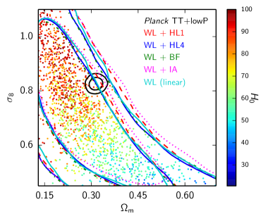
In this paper we need to be particularly careful about the contribution of nonlinear scales to $\xi^{\pm}$, since the behaviour of MG models in the nonlinear regime is not known very precisely. The standard approach is to correct the power spectrum on nonlinear scales using the Halofit fitting function. Since its inception, there have been several revisions to improve the agreement with $N$-body simulations. We use the following convention to label the particular Halofit model:

1. the original model of Smith et al. (2003);

2. an update from higher resolution $N$-body simulations, to include the effect of massive neutrinos (Bird et al. 2012);

3. an update to improve the accuracy on small scales;

4. an update from higher resolution $N$-body simulations, including DE cosmologies with constant equation of state (Takahashi et al. 2012).

Given this correction, one can scale the Weyl potential transfer functions by the ratio of the nonlinear to linear matter power spectrum

$$T_{\Phi+\Psi}(k,z)\rightarrow T_{\Phi+\Psi}(k,z)\sqrt{\frac{P_{\delta}^{\rm nonlin}(k,z)}{P_{\delta}^{\rm lin}(k,z)}}\thinspace.$$ (17)

Both (Kilbinger et al. 2013) and (Heymans et al. 2013) quote a “conservative” set of cuts to mitigate uncertainty over the nonlinear modelling scheme. For the 2D analysis of Kilbinger et al. (2013) angular scales $\theta<17\arcmin$ are excluded for $\xi^{+}$, and $\theta<54\arcmin$ for $\xi^{-}$. For the tomographic analysis of Heymans et al. (2013), angular scales $\theta<3\arcmin$ are excluded for $\xi^{+}$ for any bin combination involving the two lowest redshift bins, and no cut is applied for the highest four redshift bins. For $\xi^{-}$, angular scales $\theta<30\arcmin$ are excluded for any bin combination involving the four lowest redshift bins, and $\theta<16\arcmin$ for the highest two bins.

These cuts, however, may be insufficient for our purposes, since we are interested in extensions to $\Lambda$CDM. We therefore choose a very conservative set of cuts to mitigate the total contribution from nonlinear scales. In order to select these cuts we choose the baseline Planck TT+lowP $\Lambda$CDM cosmology as described in Planck Collaboration XIII (2015), for which one can use Eq. (15). The cuts are then chosen by considering $\Delta\chi^{2}=|\chi^{2}_{\rm lin}-\chi^{2}_{\rm nonlin}|$ of the WL likelihood as a function of angular cut. In order for this to remain $\Delta\chi^{2}<1$ for each of the Halofit versions, we find it necessary to remove $\xi^{-}$ entirely from each data set, and exclude $\theta<17\arcmin$ for $\xi^{+}$ for both the 2D and tomographic bins. We note that a similar approach to Kitching et al. (2014) could also be followed using 3D CFHTLenS data, where the choice of cut is more well defined in $k$-space, however the likelihood for this was not available at the time of this paper.

On small scales, the effects of intrinsic alignments and baryonic feedback can also become significant. In order to check the robustness of our cuts to these effects we adopt the same methodology of MacCrann et al. (2014). Using the same baseline model and choosing Halofit version 4, we scale the matter power spectrum by an active galactic nuclei (AGN) component, derived from numerical simulations (van Daalen et al. 2011), marginalizing over an amplitude $\alpha_{\rm AGN}$. The AGN baryonic feedback model has been shown by Harnois-Déraps et al. (2014) to provide the best fit to small-scale CFHTLens data. For intrinsic alignment we adopt the model of Bridle & King (2007), including the additional nonlinear alignment contributions to $\xi^{\pm}$, and again marginalizing over an amplitude $\alpha_{\rm IA}$. For more details on this procedure, we refer the reader to MacCrann et al. (2014).

The robustness of our ultra-conservative cuts to nonlinear modelling, baryonic feedback and intrinsic alignment marginalization, is illustrated in Fig. 2 for the tomographic data, with similar constraints obtained from 2D data. Assuming the same base $\Lambda$CDM cosmology, and applying priors of $\Omega_{\rm b}h^{2}=0.0223\pm 0.0009$, $n_{\rm s}=0.96\pm 0.02$, and $40\thinspace\text{km}\thinspace\text{s}^{-1}\thinspace\text{Mpc}^{-1}<H_{0}<100\thinspace\text{km}\thinspace\text{s}^{-1}\thinspace\text{Mpc}^{-1}$ to avoid over-fitting the model, we find that the WL likelihood is insensitive to nonlinear physics. We therefore choose to adopt the tomographic data with the ultra-conservative cuts as our baseline data set.

Table 1: Table of models tested in this paper. We have tested all models for the combinations: Planck, Planck+BSH, Planck+WL, Planck+BAO/RSD and Planck+WL+BAO/RSD. Throughout the text, unless otherwise specified, Planck refers to the baseline Planck TT+lowP combination. The effects of CMB lensing and Planck TT,TE,EE polarization have been tested on all runs above and are, in particular, used to constrain the amount of DE at early times.

Model           Section $$\rm{\Lambda CDM} {w} w_{0} w_{a} w w(a) w \epsilon_{\rm s} \zeta_{\rm s} \epsilon_{\infty} \mu,\eta \mu,\eta f(R)$$.           Planck Collaboration XIII (2015) Background parameterizations: .           Planck Collaboration XIII (2015) , .           Sect. 5.1.1: Figs. 3, 4, 5 higher order expansion.           Sect. 5.1.1 1-parameter .           Sect. 5.1.2: Fig. 6 PCA.           Sect. 5.1.3: Fig. 7 , , .           Sect. 5.1.4: Figs. 8, 9 Early DE.           Sect. 5.1.5: Figs. 10, 11 Perturbation parameterizations: EFT exponential.           Sect. 5.2.1: Fig. 12 EFT linear.           Sect. 5.2.1: Fig. 13 scale-independent:      DE-related.           Sect. 5.2.2: Figs. 1, 14, 15, 16, 17      time related.           Sect. 5.2.2: Figs. 14, 16 scale-dependent:.      DE-related.           Sect. 5.2.2: Fig. 18      time related.           Sect. 5.2.2 Other particular examples: DE sound speed and k-essence .           Sect. 5.3.1 Equation of state approach: .      Lorentz-violating massive gravity .           Sect. 5.3.2      Generalized scalar fields .           Sect. 5.3.2 .           Sect. 5.3.3: Figs. 19, 20 Coupled DE.           Sect. 5.3.4: Figs. 21, 22

4.4 Combining data sets

We show for convenience in Table 1 the schematic summary of models. All models have been tested for the combinations: Planck, Planck+BSH, Planck+WL, Planck+BAO/RSD and Planck+WL+BAO/RSD. Throughout the text, unless otherwise specified, Planck refers to the baseline Planck TT+lowP combination. The effects of CMB lensing and Planck TT,TE,EE polarization have been tested on all runs above and are, in particular, used to constrain the amount of DE at early times. For each of them we indicate the section in which the model is described and the corresponding figures. In addition, all combinations in the table have been tested with and without CMB lensing. The impact of Planck high-$\ell$ polarization has been tested on all models for the combination Planck+BAO+SNe+$H_{0}$.

5 Results

We now proceed by illustrating in detail the models and parameterizations described in Sect. 3, through presenting results for each of them. The structure of this section is as follows. We start in Sect. 5.1 with smooth dark energy models that are effectively parameterized by the expansion history of the Universe alone. In Sect. 5.2 we study the constraints on the presence of non-negligible dark energy perturbations, both in the context of general modified gravity models described through effective field theories and with phenomenological parameterizations of the gravitational potentials and their combinations, as illustrated in Sect. 3.2.2. The last part, Sect. 5.3, illustrates results for a range of particular examples often considered in the literature.

5.1 Background parameterizations

In this section, we consider models where DE is a generic quintessence-like component with equation of state $w\equiv p/\rho$, where $p$ and $\rho$ are the spatially averaged (background) DE pressure and density. Although it is important to include, as we do, DE perturbations, models in this section have a sound speed that is equal to the speed of light, which means that they are smooth on sub-horizon scales (see Sect. 3.1 for more details). We start with Taylor expansions and a principal component analysis of $w$ in a fluid formalism, then consider actual quintessence models parameterized through their potentials and finally study the limits that can be put on the abundance of DE density at early times. At the end of the sub-section we provide the necessary information to compress the Planck CMB power spectrum into a 4-parameter Gaussian likelihood for applications where the full likelihood is too unwieldy.

5.1.1 Taylor expansions of $w$ and $w_{0},w_{a}$ parameterization

Figure 3: Parameterization $\{w_{0},w_{a}\}$ (see Sect. 5.1.1). Marginalized posterior distributions for $w_{0}$, $w_{a}$, $H_{0}$ and $\sigma_{8}$ for various data combinations. The tightest constraints come from the Planck TT+lowP+BSH combination, which indeed tests background observations, and is compatible with $\Lambda$CDM.

If the dark energy is not a cosmological constant with $w=-1$ then there is no reason why $w$ should remain constant. In order to test a time-varying equation of state, we expand $w(a)$ in a Taylor series. The first order corresponds to the $\{w_{0},w_{a}\}$ case, also discussed in Planck Collaboration XIII (2015):

$$w(a)=w_{0}+(1-a)w_{a}\thinspace.$$ (18)

We use the parameterized post-Friedmann (PPF) model of Hu & Sawicki (2007) and Fang et al. (2008) to allow for values $w<-1$ (note that there is another PPF formalism discussed in Baker et al. (2014a)). Marginalized posterior distributions for $w_{0}$, $w_{a}$, $H_{0}$ and $\sigma_{8}$ are shown in Fig. 3 and the corresponding 2D contours can be found in Fig. 4 for $w_{a}$ vs $w_{0}$ and for $\sigma_{8}$ vs $\Omega_{\mathrm{m}}$. Results from Planck TT+lowP+BSH data are shown in blue and corresponds to the combination we consider the most secure, which in this case also gives the strongest constraints. This is expected, since the BAO and SNe data included in the BSH combination provide the best constraints on the background expansion rate.

Figure 4: Marginalized posterior distributions of the ($w_{0},w_{a}$) parameterization (see Sect. 5.1.1) for various data combinations. The best constraints come from the priority combination and are compatible with $\rm{\Lambda}$CDM. The dashed lines indicate the point in parameter space $(-1,0)$ corresponding to the $\Lambda$CDM model. CMB lensing and polarization do not significantly change the constraints. Here Planck indicates Planck TT+lowP.

Figure 5: Reconstructed equation of state $w(z)$ as a function of redshift (see Sect. 5.1.1), when assuming a Taylor expansion of $w(z)$ to first-order ($N=1$ in Eq. 19), for different combinations of the data sets. The coloured areas show the regions which contain 95 % of the models. The central blue line is the median line for Planck TT+lowP+BSH. Here Planck indicates Planck TT+lowP.

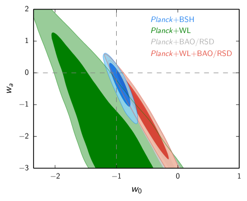
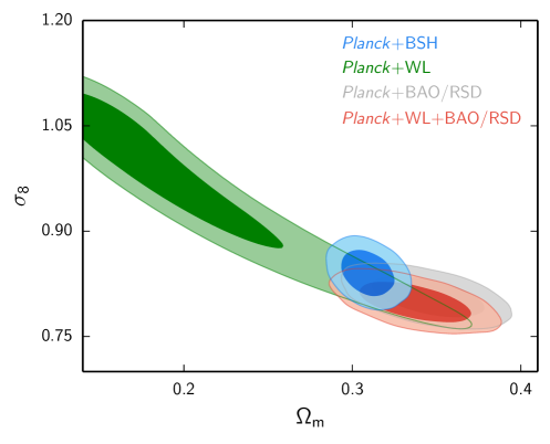
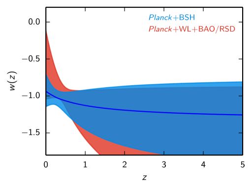
Results for weak lensing (WL) and redshift space distortions (RSD) are also shown, both separately and combined. The constraints from these probes are weaker, since we are considering a smooth dark energy model where the perturbations are suppressed on small scales. While the WL data appear to be in slight tension with $\Lambda$CDM, according to the green contours shown in Fig. 4, the difference in total $\chi^{2}$ between the best-fit in the $\{w_{0},w_{a}\}$ model and in $\Lambda$CDM for Planck TT+lowP+WL is $\Delta\chi^{2}=-5.6$, which is not very significant for 2 extra parameters (for normal errors a $2\thinspace\sigma$ deviation corresponds to a $\chi^{2}$ absolute difference of 6.2). The WL contributes a $\Delta\chi^{2}$ of $-2.0$ and the $\Delta\chi^{2}_{\rm{CMB}}=-3.3$ (virtually the same as when using Planck TT+lowP alone, for which $\Delta\chi^{2}_{\rm{CMB}}=-3.2$, which seems to indicate that WL is not in tension with Planck TT+lowP within a ($w_{0},w_{a}$) cosmology). However, as also discussed in Planck Collaboration XIII (2015), these data combinations prefer very high values of $H_{0}$, which is visible also in the third panel of Fig. 3. The combination Planck TT+lowP+BSH, on the other hand, is closer to $\Lambda$CDM, with a total $\chi^{2}$ difference between ($w_{0},w_{a}$) and $\Lambda$CDM  of only $-0.8$. We also show in Fig. 5 the equation of state reconstructed as a function of redshift from the linear expansion in the scale factor $a$ for different combinations of data.

One might wonder whether it is reasonable to stop at first order in $w(a)$. We have therefore tested a generic expansion in powers of the scale factor up to order $N$:

$$w(a)=w_{0}+\sum_{i=1}^{N}(1-a)^{i}w_{i}\thinspace.$$ (19)

We find that all parameters are very stable when allowing higher order polynomials; the $w_{i}$ parameters are weakly constrained and going from $N=1$ (the linear case) to $N=2$ (quadratic case) to $N=3$ (cubic expansion) does not improve the goodness of fit and stays compatible with $\rm{\Lambda CDM}$, which indicates that a linear parameterization is sufficient.

5.1.2 1-parameter varying $w$

A simple example of a varying $w$ model that can be written in terms of one extra parameter only (instead of $w_{0},w_{a}$) was proposed in Gott & Slepian (2011); Slepian et al. (2014), motivated in connection to a DE minimally-coupled scalar field, slowly rolling down a potential $\frac{1}{2}m^{2}\phi^{2}$, analogous to the one predicted in chaotic inflation (Linde 1983). More generally, one can fully characterize the background by expanding a varying equation of state $w(z)\equiv-1+\delta w(z)\approx-1+\delta w_{0}\times H_{0}^{2}/H^{2}(z)$, where:

$$\frac{H^{2}(z)}{H_{0}^{2}}\approx\Omega_{\mathrm{m}}(1+z)^{3}+\Omega_{\mathrm{de}}\left[\frac{(1+z)^{3}}{\Omega_{\mathrm{m}}(1+z)^{3}+\Omega_{\mathrm{de}}}\right]^{\delta w_{0}/\Omega_{\mathrm{de}}}\thinspace,$$ (20)

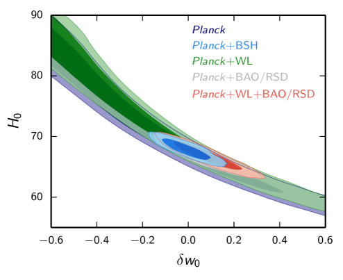
at first order in $\delta w_{0}$, which is then the only extra parameter. Marginalized posterior contours in the plane $h$–$\delta w_{0}$ are shown in Fig. 6. The tightest constraints come from the combination Planck TT+lowP+lensing+BSH that gives $\delta w_{0}=-0.008\pm 0.068$ at 68 % confidence level, which slightly improves constraints found by Aubourg et al. (2014).

Figure 6: Marginalized posterior contours in the $h$–$\delta w_{0}$ plane are shown for 1-parameter varying $w$ models (see Sect. 5.1.2) for different data combinations. Here Planck indicates Planck TT+lowP.

5.1.3 Principal Component Analysis on w(z)

A complementary way to measure the evolution of the equation of state, which is better able to model rapid variations, proceeds by choosing $w$ in $N$ fixed bins in redshift and by performing a principal component analysis to uncorrelate the constraints. We consider $N=4$ different bins in $z$ and assume that $w$ has a constant value $p_{i}$ in each of them. We then smooth the transition from one bin to the other such that:

$$w(z) = p_{i-1}+\Delta w\left(\tanh\left[\frac{z-z_{i}}{s}\right]+1\right)\ \textrm{for}\thinspace z<z_{i}\thinspace,\ \textrm{i $\epsilon$ \{1, 4\}},$$ (21)

with $\Delta w\equiv(p_{i}-p_{i-1})/{2}$, a smoothing scale $s=0.02$, and a binning $z_{i}=(0,0.2,0.4,0.6,1.8)$. We have tested also a larger number of bins (up to $N=18$) and have found no improvement in the goodness of fit.

The constraints on the vector $\@vec{p}_{i}(i=1,\ldots,N)$ of values that $w(z)$ can assume in each bin is difficult to interpret, due to the correlations between bins. To uncorrelate the bins, we perform a principal component analysis (Huterer & Starkman 2003; Huterer & Cooray 2005; Said et al. 2013). We first run COSMOMC (Lewis & Bridle 2002) on the original binning values $\@vec{p}_{i}$; then extract the covariance matrix that refers to the parameters we want to constrain:

$$C\equiv\left\langle pp^{\rm T}\right\rangle-\langle p\rangle\langle p^{\rm T}\rangle,$$ (22)

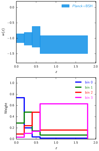
where $p$ is the vector of parameters $p_{i}$ and $p^{\rm T}$ is its transpose. We calculate the Fisher matrix, $F=C^{-1}$, and diagonalize it, $F=O^{\rm T}\Lambda O$, where $\Lambda$ is diagonal and $O$ is the orthogonal matrix whose columns are the eigenvectors of the Fisher matrix. We then define $\widetilde{W}=O^{\rm T}\Lambda^{1/2}O$ (e.g., Huterer & Cooray 2005) and normalize this such that its rows sum up to unity; this matrix can be used to find the new vector $q=\widetilde{W}p$ of uncorrelated parameters that describe $w(z)$. This choice of $\tilde{W}$ has been shown to be convenient, since most of the weights (i.e., the rows of $\widetilde{W}$) are found to be positive and fairly well localized in redshift. In Fig. 7 (lower panel) we show the weights for each bin as a function of redshift. Because they overlap only partially, we can assume the binning to be the same as the original one and attach to each of them error bars corresponding to the mean and standard deviations of the $q$ values. The result is shown in Fig. 7, top panel. The equation of state is compatible with the $\Lambda$CDM value $w=-1$. Note however that this plot contains more information than a Taylor expansion to first order.

Figure 7: PCA analysis constraints (described in Sect. 5.1.3). The top panel shows the reconstructed equation of state $w(z)$ after the PCA analysis. Vertical error bars correspond to mean and standard deviations of the $q$ vector parameters, while horizontal error bars are the amplitude of the original binning. The bins are not exactly independent but are rather smeared out as illustrated in the bottom panel. The bottom panel shows the PCA corresponding weights on $w(z)$ as a function of redshift for the combination Planck TT+lowP+BSH. In other words, error bars in the top panel correspond therefore to the errors in the $q$ parameters, which are linear combinations of the $p$ parameters, i.e. a smeared out distribution with weights shown in the lower panel.

5.1.4 Parameterization for a weakly-coupled canonical scalar field.

We continue our investigation of background parameterizations by considering a slowly rolling scalar field. In this case, as in inflation, we can avoid writing down an explicit potential $V(\phi)$ and instead parameterize $w(a)$ at late times, in the presence of matter, as (Huang et al. 2011)

$$w=-1+\frac{2}{3}\epsilon_{\rm s}F^{2}\left(\frac{a}{a_{\rm de}}\right)\thinspace,$$ (23)

where the “slope parameter” $\epsilon_{\rm s}$ is defined as:

$$\epsilon_{\rm s}\equiv\left.\epsilon_{\rm V}\right|_{a=a_{\rm de}}\thinspace,$$ (24)

with $\epsilon_{\rm V}\equiv(\frac{d\ln V}{d\phi})^{2}M_{\text{P}}^{2}/2$ being a function of the slope of the potential. Here $M_{\text{P}}\equiv{1}/{\sqrt{8\pi G}}$ is the reduced Planck mass and $a_{\rm de}$ is the scale factor where the total matter and DE densities are equal. The function $F(x)$ in Eq. (23) is defined as:

$$F(x)\equiv\frac{\sqrt{1+x^{3}}}{x^{3/2}}-\frac{\ln{\left(x^{3/2}+\sqrt{1+x^{3}}\right)}}{x^{3}}\thinspace.$$ (25)

Eq. (23) parameterizes $w(a)$ with one parameter $\epsilon_{\rm s}$, while $a_{\rm de}$ depends on $\Omega_{\mathrm{m}}$ and $\epsilon_{\rm s}$ and can be derived using an approximated fitting formula that facilitates numerical computation (Huang et al. 2011). Positive (negative) values of $\epsilon_{\rm s}$ correspond to quintessence (phantom) models.

Eq. (23) is only valid for late-Universe slow-roll ($\epsilon_{\rm V}\lesssim 1$ and $\eta_{V}\equiv M_{\text{P}}^{2}{V^{\prime\prime}}/{V}\ll 1$) or the moderate-roll ($\epsilon_{\rm V}\lesssim 1$ and $\eta_{V}\lesssim 1$) regime. For quintessence models, where the scalar field rolls down from a very steep potential, at early times $\epsilon_{\rm V}(a)\gg 1$, however the fractional density $\Omega_{\phi}(a)\rightarrow 0$ and the combination $\epsilon_{\rm V}(a)\Omega_{\phi}(a)$ aprroaches a constant, defined to be a second parameter $\epsilon_{\infty}\equiv\lim_{a\rightarrow 0}\epsilon_{\rm V}(a)\Omega_{\phi}(a)$.

One could also add a third parameter $\zeta_{\rm s}$ to capture the time-dependence of $\epsilon_{\rm V}$ via corrections to the functional dependence of $w(a)$ at late time. This parameter is defined as the relative difference of $d\sqrt{\epsilon_{\rm V}\Omega_{\phi}}/dy$ at $a=a_{\rm de}$ and at $a\rightarrow 0$, where $y\equiv(a/a_{\rm de})^{3/2}/\sqrt{1+(a/a_{\rm de})^{3}}$. If $\epsilon_{\infty}\ll 1$, $\zeta_{\rm s}$ is proportional to the second derivative of $\ln V(\phi)$, but for large $\epsilon_{\infty}$, the dependence is more complicated (Huang et al. 2011). In other words, while $\epsilon_{\rm s}$ is sensitive to the late time evolution of $1+w(a)$, $\epsilon_{\infty}$ captures its early time behaviour. Quintessence/phantom models can be mapped into $\epsilon_{\rm s}$–$\epsilon_{\infty}$ space and the classification can be further refined with $\zeta_{\rm s}$. For $\Lambda$CDM, all three parameters are zero.

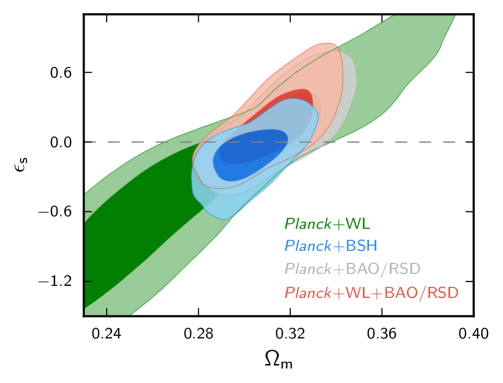
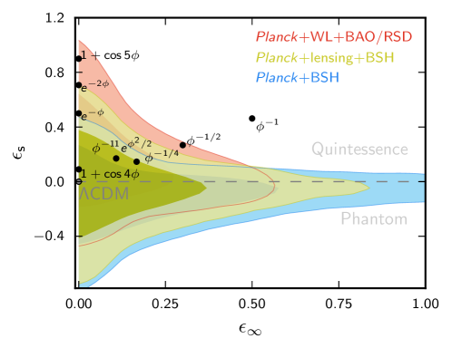
In Fig. 8 we show the marginalized posterior distributions at 68.3 % and 95.4 % confidence levels in the parameter space $\epsilon_{\rm s}$–$\Omega_{\mathrm{m}}$, marginalizing over the other parameters. In Fig. 9 we show the current constraints on quintessence models projected in $\epsilon_{\rm s}$–$\epsilon_{\infty}$ space. The constraints are obtained by marginalizing over all other cosmological parameters. The models here include exponentials $V=V_{0}\exp(-\lambda\phi/M_{\text{P}})$ (Wetterich 1988), cosines from pseudo-Nambu Goldstone bosons (pnGB) $V=V_{0}[1+\cos({\lambda\phi/M_{\text{P}}})]$ (Frieman et al. 1995; Kaloper & Sorbo 2006), power laws $V=V_{0}(\phi/M_{\text{P}})^{-n}$ (Ratra & Peebles 1988), and models motivated by supergravity (SUGRA) $V=V_{0}(\phi/M_{\text{P}})^{-\alpha}\exp{[(\phi/M_{\text{P}})^{2}]}$ (Brax & Martin 1999). The model projection is done with a fiducial $\Omega_{\mathrm{m}}=0.3$ cosmology. We have verified that variations of 1 % compared to the fiducial $\Omega_{\mathrm{m}}$ lead to negligible changes in the constraints.

Mean values and uncertainties for a selection of cosmological parameters are shown in Table 2, for both the 1-parameter case (i.e., $\epsilon_{\rm s}$ only, with $\epsilon_{\infty}=0$ and $\zeta_{\rm s}=0$, describing “thawing” quintessence/phantom models, where $\dot{\phi}=0$ in the early Universe) and the 3-parameter case (general quintessence/phantom models where an early-Universe fast-rolling phase is allowed). When we vary the data sets and theoretical prior (between the 1-parameter and 3-parameter cases), the results are all compatible with $\Lambda$CDM and mutually compatible with each other. Because $\epsilon_{\rm s}$ and $\epsilon_{\infty}$ are correlated, caution has to be taken when looking at the marginalized constraints in the table. For instance, the constraint on $\epsilon_{\rm s}$ is tighter for the 3-parameter case, because in this case flatter potentials are preferred in the late Universe in order to slow-down larger $\dot{\phi}$ from the early Universe. A better view of the mutual consistency can be obtained from Fig. 9. We find that the addition of polarization data does not have a large impact on these DE parameters. Adding polarization data to Planck+BSH shifts the mean of $\epsilon_{\rm s}$ by $-1/6\thinspace\sigma$ and reduces the uncertainty of $\epsilon_{\rm s}$ by 20 %, while the 95 % upper bound on $\epsilon_{\infty}$ remains unchanged.

Figure 8: Marginalized posterior distributions showing 68 % and 95 % C.L. constraints on $\Omega_{\mathrm{m}}$ and $\epsilon_{\rm s}$ for scalar field models (see Sect. 5.1.4). The dashed line for $\epsilon_{\rm s}=0$ is the $\Lambda$CDM model. Here Planck indicates Planck TT+lowP.

Figure 9: Marginalized posterior distributions at 68 % C.L. and 95 % C.L. in the parameter space of $\epsilon_{\rm s}$ and $\epsilon_{\infty}$ for scalar field modes (see Sect. 5.1.4). We have computed $\epsilon_{\rm s}$ and $\epsilon_{\infty}$ for various quintessence potentials $V(\phi)$, with the functional forms of $V(\phi)$ labelled on the figure. The field $\phi$ is in reduced Planck mass $M_{\text{P}}$ units. The normalization of $V(\phi)$ is computed using $\Omega_{\mathrm{m}}=0.3$. Here Planck indicates Planck TT+lowP.

Table 2: Marginalized mean values and 68 % CL errors for a selection of cosmological parameters for the weakly-coupled scalar field parameterization described in the text (Sect. 5.1.4). Here “1-param” in the first column refers to the priors $\epsilon_{\infty}=0$ and $\zeta_{\rm s}=0$ (slow- or moderate-roll “thawing” models).

5.1.5 Dark energy density at early times

Quintessence models can be divided into two classes, namely cosmologies with or without DE at early times. Although the equation of state and the DE density are related to each other, it is often convenient to think directly in terms of DE density rather than the equation of state. In this section we provide a more direct estimate of how much DE is allowed by the data as a function of time. A key parameter for this purpose is $\Omega_{\rm{e}}$, which measures the amount of DE present at early times (“early dark energy,” EDE) (Wetterich 2004). Early DE parameterizations encompass features of a large class of dynamical DE models. The amount of early DE influences CMB peaks and can be strongly constrained when including small-scale measurements and CMB lensing. Assuming a constant fraction of $\Omega_{\rm{e}}$ until recent times (Doran & Robbers 2006), the DE density is parameterized as:

$$\Omega_{\mathrm{de}}(a)=\frac{\Omega_{\mathrm{de}}^{0}-\Omega_{\rm{e}}(1-a^{-3w_{0}})}{\Omega_{\mathrm{de}}^{0}+\Omega_{\mathrm{m}}^{0}a^{3w_{0}}}+\Omega_{\rm{e}}(1-a^{-3w_{0}})\thinspace.$$ (26)

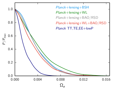
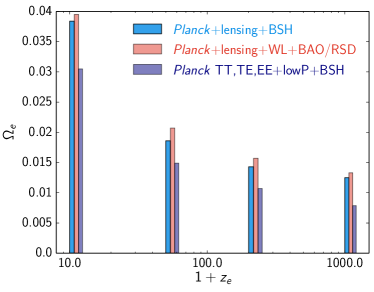
This expression requires two parameters in addition to those of $\rm{\Lambda}$CDM, namely $\Omega_{\rm{e}}$ and $w_{0}$, while $\Omega_{\mathrm{m}}^{0}=1-\Omega_{\mathrm{de}}^{0}$ is the present matter abundance. The strongest constraints to date were discussed in (Planck Collaboration XVI 2014), finding $\Omega_{\rm{e}}<0.010$ at 95 % CL using Planck combined with WMAP polarization. Here we update the analysis using Planck 2015 data. In Fig. 10 we show marginalized posterior distributions for $\Omega_{\rm{e}}$ for different combination of data sets; the corresponding marginalized limits are shown in Table 3, improving substantially current constraints, especially when the Planck TT,TE,EE+lowP polarization is included, leading to $\Omega_{\rm{e}}<0.0036$ at $95\%$ confidence level for Planck TT,TE,EE+lowP+BSH.

Figure 10: Marginalized posterior distributions for $\Omega_{\rm{e}}$ for the early DE parameterization in (26) and for different combinations of data (see Sect. 5.1.5). Here Planck indicates Planck TT+lowP.

Table 3: Marginalized 95 % limits on $\Omega_{\rm{e}}$ and $w_{0}$ for the early DE parameterization in Eq. (26) and different combinations of data (see Sect. 5.1.5). Including high-$\ell$ polarization significantly tightens the bounds.

As first shown in Pettorino et al. (2013), bounds on $\Omega_{\rm{e}}$ can be weaker if DE is present only over a limited range of redshifts. In particular, EDE reduces structure growth in the period after last scattering, implying a smaller number of clusters as compared to $\Lambda$CDM, and therefore a weaker lensing potential to influence the anisotropies at high $\ell$. It is possible to isolate this effect by switching on EDE only after last scattering, at a scale factor $a_{\rm{e}}$ (or equivalently for redshifts smaller than $z_{\rm{e}}$). Here we adopt the parameterization “EDE3” proposed in Pettorino et al. (2013) to which we refer for more details:

$$\Omega_{\mathrm{de}}(a)=\begin{cases}\frac{\displaystyle\Omega_{\rm{de}0}}{\displaystyle\Omega_{\rm{de0}}+\Omega_{\rm{m0}}a^{-3}+\Omega_{\rm{r0}}a^{-4}}&\mbox{for }a\leq a_{\rm{e}}\thinspace;\\[10.0pt] \Omega_{\rm{e}}&\mbox{for }a_{\rm{e}}<a<a_{\rm{c}}\thinspace:\\[5.0pt] \frac{\displaystyle\Omega_{\rm{de0}}}{\displaystyle\Omega_{\rm{de0}}+\Omega_{\rm{m0}}a^{-3}+\Omega_{\rm{r0}}a^{-4}}&\mbox{for }a>a_{\rm{c}}\thinspace.\end{cases}$$ (27)

In this case, early dark energy is present in the time interval $a_{\rm{e}}<a<a_{\rm{c}}$, while outside this interval it behaves as in $\Lambda$CDM, including the radiation contribution, unlike in Eq. (26). During that interval in time, there is a non-negligible EDE contribution, parameterized by $\Omega_{\rm{e}}$. The constant $a_{\rm{c}}$ is fixed by continuity, so that the parameters {$\Omega_{\rm{e}},a_{\rm{e}}$} fully determine how much EDE there was and how long its presence lasted. We choose four fixed values of $a_{\rm{e}}$ corresponding to $z_{\rm{e}}=10$, $50$, $200$ and $1000$ and include $\Omega_{\rm{e}}$ as a free parameter in MCMC runs for each value of $a_{\rm{e}}$. Results are shown in Fig. 11 where we plot $\Omega_{\rm{e}}$ as a function of the redshift $z_{\rm{e}}$ at which DE starts to be non-negligible. The smaller the value of $z_{\rm{e}}$, the weaker are the constraints, though still very tight, with $\Omega_{\rm{e}}\la 2\thinspace\%\thinspace\thinspace(95\thinspace\%$ CL) for $z_{\rm{e}}\approx 50$.

Figure 11: Amount of DE at early times $\Omega_{e}$ as a function of the redshift $z_{e}$ after which early DE is non-negligible (see Eq. (27), Sect. 5.1.5) for different combinations of data sets. The heights of the columns give the limit at 95 % CL on $\Omega_{e}$, as obtained from Monte Carlo runs for the values $z_{e}=10$, $50$, $200$ and $1000$. The width of the columns has no physical meaning and is just due to plotting purposes. Here Planck indicates Planck TT+lowP.

5.1.6 Compressed likelihood

Before concluding the set of results on background parameterizations, we discuss here how to reduce the full likelihood information to few parameters. As discussed for example in Kosowsky et al. (2002) and Wang & Mukherjee (2007), it is possible to compress a large part of the information contained in the CMB power spectrum into just a few numbers: here we use specifically the CMB shift parameter $R$ (Efstathiou & Bond 1999), the angular scale of the sound horizon at last scattering $\ell_{\rm A}$ (or equivalently $\theta_{\ast}$), as well the baryon density $\omega_{\rm b}$ and the scalar spectral index $n_{\rm s}$. The first two quantities are defined as

$$R\equiv\sqrt{\Omega_{\mathrm{m}}H_{0}^{2}}\thinspace D_{\rm A}(z_{\ast})/c\thinspace\thinspace\thinspace\thinspace,\thinspace\thinspace\thinspace\thinspace\ \ell_{\rm A}\equiv\pi D_{\rm A}(z_{\ast})/r_{\rm s}(z_{\ast})=\pi/\theta_{\ast}\thinspace,$$ (28)

where $D_{\rm A}(z)$ is the comoving angular diameter distance to redshift $z$, $z_{\ast}$ is the redshift for which the optical depth is unity and $r_{\rm s}(z_{\ast})=r_{\ast}$ is the comoving size of the sound horizon at $z_{\ast}$. These numbers are effectively observables and they apply to models with either non-zero curvature or a smooth DE component (Mukherjee et al. 2008). It should be noted, however, that the constraints on these quantities, especially on $R$, are sensitive to changes in the growth of perturbations. This can be seen easily with the help of the “dark degeneracy” (Kunz 2009), i.e., the possibility to absorb part of the dark matter into the dark energy, which changes $\Omega_{\mathrm{m}}$ without affecting observables. For this reason the compressed likelihood presented here cannot be used for models with low sound speed or modifications of gravity (and is therefore located at the end of this “background” section).

Table 4: Compressed likelihood discussed in Sect. 5.1.6. The left columns give the marginalized mean values and standard deviation for the parameters of the compressed likelihood for Planck TT+lowP, while the right columns present the normalized covariance or correlation matrix $\@tens{D}$ for the parameters of the compressed likelihood for Planck TT+lowP. The covariance matrix $\@tens{C}$ is then given by $\@tens{C}_{ij}=\sigma_{i}\sigma_{j}\@tens{D}_{ij}$ (without summation), where $\sigma_{i}$ is the standard deviation of parameter $i$. While the upper values were derived for $w$CDM and are consistent with those of $\rm{\Lambda CDM}$ and the $\{w_{0},w_{a}\}$ model, we marginalized over the amplitude of the lensing power spectrum for the lower values, which leads to a more conservative compressed likelihood.

The marginalized mean values and 68 % confidence intervals for the compressed likelihood values are shown in Table 4 for Planck TT+lowP. The posterior distribution of $\{R,\ell_{\rm A},\omega_{\rm b},n_{\rm s}\}$ is approximately Gaussian, which allows us to specify the likelihood easily by giving the mean values and the covariance matrix, as derived from a Monte Carlo Markov chain (MCMC) approach, in this case from the grid chains for the $w$CDM model. Since these quantities are very close to observables directly derivable from the data, and since smoothly parameterized DE models are all compatible with the Planck observations to a comparable degree, they lead to very similar central values and essentially the same covariance matrix. The Gaussian likelihood in $\{R,\ell_{\rm A},\omega_{\rm b},n_{\rm s}\}$ given by Table 4 is thus useful for combining Planck temperature and low-$\ell$ polarization data with other data sets and for inclusion in Fisher matrix forecasts for future surveys. This is especially useful when interested in parameters such as $\{w_{0},w_{a}\}$, for which the posterior is very non-Gaussian and cannot be accurately represented by a direct covariance matrix (as can be seen in Fig. 4).

The quantities that make up the compressed likelihood are supposed to be “early universe observables” that describe the observed power spectrum and are insensitive to late time physics. However, lensing by large-scale structure has an important smoothing effect on the $C_{\ell}$ and is detected at over $10\thinspace\sigma$ in the power spectrum (see section 5.2 of Planck Collaboration XIII (2015)). We checked by comparing different MCMC chains that the compressed likelihood is stable for $\rm{\Lambda CDM}$, $w$CDM and the $\{w_{0},w_{a}\}$ model. However, the “geometric degeneracy” in curved models is broken significantly by the impact of CMB lensing on the power spectrum (see Fig. 25 of Planck Collaboration XIII 2015) and for non-flat models one needs to be more careful. For this reason we also provide the ingredients for the compressed likelihood marginalized over the amplitude $A_{\rm L}$ of the lensing power spectrum in the lower part of Table 4. Marginalizing over $A_{\rm L}$ increases the errors in some variables by over 20 % and slightly shifts the mean values, giving a more conservative choice for models where the impact of CMB lensing on the power spectrum is non-negligible.

We notice that the constraints on $\{R,\ell_{\rm A},\omega_{\rm b},n_{\rm s}\}$ given in Table 4 for Planck TT+lowP data are significantly weaker than those predicted by table II of Mukherjee et al. (2008), which were based on the “Planck Blue Book” specifications Planck Collaboration (2005). This is because these forecasts also used high-$\ell$ polarization. If we derive the actual Planck covariance matrix for the Planck TT,TE,EE+lowP likelihood then we find constraints that are about 50 % smaller than those given above, and are comparable and even somewhat stronger than those quoted in Mukherjee et al. (2008). The mean values have of course shifted to represent what Planck has actually measured.

5.2 Perturbation parameterizations

Up to now we have discussed in detail the ensemble of background parameterizations, in which DE is assumed to be a smooth fluid, minimally interacting with gravity. General modifications of gravity, however, change both the background and the perturbation equations, allowing for contribution to clustering (via a sound speed different than unity) and anisotropic stress different from zero. Here we illustrate results for perturbation degrees of freedom, approaching MG from two different perspectives, as discussed in Sect. 3. First we discuss results for EFT cosmologies, with a “top-down” approach that starts from the most general action allowed by symmetry and selects from there interesting classes belonging to so-called “Horndeski models”, which, as mentioned in Sect. 3.2.1, include almost all stable scalar-tensor theories, universally coupled, with second-order equations of motion in the fields. We then proceed by parameterizing directly the gravitational potentials and their combinations, as illustrated in Sect. 3.2.2. In this way we can test more phenomenologically their effect on lensing and clustering, in a “bottom-up” approach from observations to theoretical models.

5.2.1 Modified gravity: EFT and Horndeski models

The first of the two approaches described in Sect. 3.2.1 adopts effective field theory (EFT) to investigate DE (Gleyzes et al. 2013; Gubitosi et al. 2013), based on the action of Eq. (2). The parameters that appear in the action, when choosing the nine time-dependent functions $\{\Omega,c,\Lambda,\bar{M}_{1}^{3},\bar{M}_{2}^{4},\bar{M}_{3}^{2},M_{2}^{4},\hat{M}^{2},m_{2}^{2}\}$, describe the effective DE. The full background and perturbation equations for this action have been implemented in the publicly available Boltzmann code EFTCAMB (Hu et al. 2014; Raveri et al. 2014) . Given an expansion history (which we fix to be $\Lambda$CDM, i.e., effectively $w\thinspace{=}\thinspace-1$) and an EFT function $\Omega(a)$, EFTCAMB computes $c$ and $\Lambda$ from the Friedmann equations and the assumption of spatial flatness (Hu et al. 2014). As we have seen in Sect. 5.1, for smooth DE models the constraints on the DE equation of state are compatible with $w\thinspace{=}\thinspace-1$; hence this choice is not a limitation for the following analysis. In addition, EFTCAMB uses a set of stability criteria in order to specify whether a given model is stable and ghost-free, i.e. without negative energy density for the new degrees of freedom. This will automatically place a theoretical prior on the parameter space while performing the MCMC analysis.

The remaining six functions, $\bar{M}_{1}^{3}$, $\bar{M}_{2}^{4}$, $\bar{M}_{3}^{2}$, $M_{2}^{4}$, $\hat{M}^{2}$, $m_{2}^{2}$, are internally redefined in terms of the dimensionless parameters $\alpha_{i}$ with $i$ running from $1$ to $6$:

$$\alpha_{1}^{4} =\frac{M^{4}_{2}}{m_{0}^{2}H_{0}^{2}}, \alpha_{2}^{3} =\frac{\bar{M}^{3}_{1}}{m_{0}^{2}H_{0}}, \alpha_{3}^{2} =\frac{\bar{M}^{2}_{2}}{m_{0}^{2}},$$

$$\alpha_{4}^{2} =\frac{\bar{M}^{2}_{3}}{m_{0}^{2}}, \alpha_{5}^{2} =\frac{\hat{M}^{2}}{m_{0}^{2}}, \alpha_{6}^{2} =\frac{m^{2}_{2}}{m_{0}^{2}}.$$

We will always demand that

$$m_{2}^{2} = 0\ (\textrm{or equivalently}\ \alpha_{6}^{2}=0),$$ (29)

$$\bar{M}_{3}^{2} = -\bar{M}_{2}^{2}\ (\textrm{or equivalently}\ \alpha_{4}^{2}=-\alpha_{3}^{2}),$$ (30)

which eliminates models containing higher-order spatial derivatives (Gleyzes et al. 2013, 2014). In this case the nine functions of time discussed above reduce to a minimal set of five functions of time that can be labelled {$\alpha_{\mathrm{M}},\alpha_{\mathrm{K}},\alpha_{\mathrm{B}},\alpha_{\mathrm{T}},\alpha_{\mathrm{H}}$}, in addition to the Planck mass $M_{\ast}^{2}$ (the evolution of which is determined by $H$ and $\alpha_{M}$), and an additional function of time describing the background evolution, e.g., $H(a)$. The former are related to the EFT functions via the following relations:

$$M_{\ast}^{2} = m_{0}^{2}\Omega+\bar{M}_{2}^{2};$$ (31)

$$M_{\ast}^{2}H\alpha_{\mathrm{M}} = m_{0}^{2}\dot{\Omega}+\dot{\bar{M}}_{2}^{2};$$ (32)

$$M_{\ast}^{2}H^{2}\alpha_{\mathrm{K}} = 2c+4M_{2}^{4};$$ (33)

$$M_{\ast}^{2}H\alpha_{\mathrm{B}} = -m_{0}^{2}\dot{\Omega}-\bar{M}_{1}^{3};$$ (34)

$$M_{\ast}^{2}\alpha_{\mathrm{T}} = -\bar{M}_{2}^{2};$$ (35)

$$M_{\ast}^{2}\alpha_{\mathrm{H}} = 2\hat{M}^{2}-\bar{M}_{2}^{2}.$$ (36)

These five $\alpha$ functions are closer to a physical description of the theories under investigation (Bellini & Sawicki 2014). For example: $\alpha_{T}$ enters in the equation for gravitational waves, affecting their speed and the position of the primordial peak in $B$-mode polarization; $\alpha_{M}$ affects the lensing potential, but also the amplitude of the primordial polarization peak in $B$-modes (Amendola et al. 2014; Raveri et al. 2014; Pettorino & Amendola 2014). It is then possible to relate the desired choice for the Horndeski variables to an appropriate choice of the EFT functions,

$$\partial_{\tau}(M_{\ast}^{2}) = {\cal H}M_{\ast}^{2}\alpha_{\mathrm{M}},$$ (37)

$$m_{0}^{2}(\Omega+1) = (1+\alpha_{\mathrm{T}})M_{\ast}^{2},$$ (38)

$$\bar{M}_{2}^{2} = -\alpha_{\mathrm{T}}M_{\ast}^{2},$$ (39)

$$4M_{2}^{4} = M_{\ast}^{2}{\cal H}^{2}\alpha_{\mathrm{K}}-2c,$$ (40)

$$\bar{M}_{1}^{3} = -M_{\ast}^{2}{\cal H}\alpha_{\mathrm{B}}+m_{0}^{2}\dot{\Omega},$$ (41)

$$2\hat{M}^{2} = M_{\ast}^{2}(\alpha_{\mathrm{H}}-\alpha_{\mathrm{T}}),$$ (42)

where ${\cal{H}}$ is the conformal Hubble function, $m_{0}$ the bare Planck mass and $M_{\ast}$ the effective Plank mass. Fixing $\alpha_{\mathrm{M}}$ corresponds to fixing $M_{\ast}$ through Eq. (37). Once $\alpha_{\mathrm{T}}$ has been chosen, $\Omega$ is obtained from Eq. (38). Finally, $\alpha_{\mathrm{B}}$ determines $\bar{M}_{1}^{3}$ via Eq. (41), while the choice of $\alpha_{\mathrm{H}}$ fixes $\hat{M}^{2}$ via Eq. (42). In this way, our choice of the EFT functions can be guided by the selection of different “physical” scenarios, corresponding to turning on different Horndeski functions.

To avoid possible consistency issues with higher derivatives, we set $\bar{M}_{3}^{2}=\bar{M}_{2}^{2}=0$ in order to satisfy Eq. (30). From Eq. (39) and Eq. (31) this implies $\alpha_{\mathrm{T}}=0$, so that tensor waves move with the speed of light. In addition, we set $\alpha_{\mathrm{H}}=0$ so as to remain in the original class of Horndeski theories. As a consequence, $\hat{M}^{2}=0$ from Eq. (42) and $M_{*}^{2}=m_{0}^{2}(1+\Omega)$ from Eq. (31). For simplicity we also turn off all other higher-order EFT operators and set $\bar{M}_{1}^{3}=M_{2}^{4}=0$. Comparing Eq. (32) and Eq. (41), this implies $\alpha_{\mathrm{B}}=-\alpha_{\mathrm{M}}$.

In summary, in the following we consider Horndeski models in which $\alpha_{\mathrm{M}}=-\alpha_{\mathrm{B}}$, $\alpha_{\mathrm{K}}$ is fixed by Eq. (34), with $M_{2}$ = 0 as a function of $c$ and $\alpha_{\mathrm{T}}=\alpha_{\mathrm{H}}=0$. We are thus considering non-minimally coupled “K-essence” type models, similar to the ones discussed in Sawicki et al. (2013).

The only free function in this case is $\alpha_{\mathrm{M}}$, which is linked to $\Omega$ through:

$$\alpha_{M}=\frac{a}{\Omega+1}\frac{\rm{d}\Omega}{\rm{d}a}\thinspace.$$ (43)

By choosing a non-zero $\alpha_{\mathrm{M}}$ (and therefore a time evolving $\Omega$) we introduce a non-minimal coupling in the action (see Eq. 2), which will lead to non-zero anisotropic stress and to modifications of the lensing potential, typical signatures of MG models. Here we will use a scaling ansatz, $\alpha_{\mathrm{M}}=\alpha_{\mathrm{M0}}a^{\beta}$, where $\alpha_{\mathrm{M0}}$ is the value of $\alpha_{\mathrm{M}}$ today, and $\beta>0$ determines how quickly the modification of gravity decreases in the past.

Integrating Eq. (43) we obtain

$$\Omega(a)=\exp\left\{\frac{\alpha_{\mathrm{M0}}}{\beta}a^{\beta}\right\}-1,$$ (44)

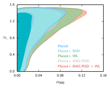
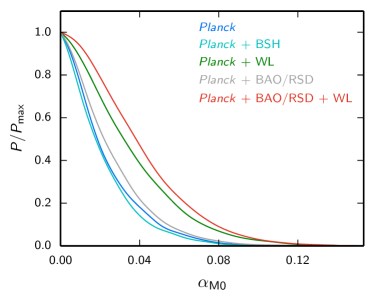
which coincides with the built-in exponential model of EFTCAMB for $\Omega_{0}=\alpha_{\mathrm{M0}}/\beta$. The marginalized posterior distributions for the two parameters $\Omega_{0}$ and $\beta$ are plotted in Fig. 12 for different combinations of data. For $\alpha_{\mathrm{M0}}=0$ we recover $\rm{\Lambda CDM}$. For small values of $\Omega_{0}$ and for $\beta=1$, the exponential reduces to the built-in linear evolution in EFTCAMB,

$$\Omega(a)=\Omega_{0}\thinspace a\thinspace.$$ (45)

The results of the MCMC analysis are shown in Table 5. For both the exponential and the linear model we use a flat prior $\Omega_{0}\in[0,1]$. For the scaling exponent $\beta$ of the exponential model we use a flat prior $\beta\in(0,3]$. For $\beta\rightarrow 0$ the MG parameter $\alpha_{M}$ remains constant and does not go to zero in the early Universe, while for $\beta=3$ the scaling would correspond to M functions in the action (2) which are of the same order as the relative energy density between DE and the dark matter background, similar to the suggestion in Bellini & Sawicki (2014). An important feature visible in Fig. 12 is the sharp cutoff at $\beta\approx 1.5$. This cutoff is due to “viability conditions” that are enforced by EFTCAMB and that reject models due to a set of theoretical criteria (see Hu et al. (2014) for a full list of theoretical priors implemented in EFTCAMB). Disabling some of these conditions allows to extend the acceptable model space to larger $\beta$, and we find that the constraints on $\alpha_{M0}$ continue to weaken as $\beta$ grows further, extending Fig. 12 in the obvious way. We prefer however to use here the current public EFTCAMB version without modifications. A better understanding of whether all stability conditions implemented in the code are really necessary or exclude a larger region than necessary in parameter space will have to be addressed in the future. The posterior distribution of the linear evolution for $\Omega$ is shown in Fig. 13 and is compatible with $\rm{\Lambda CDM}$. Finally, it is interesting to note that in both the exponential and the linear expansion, the inclusion of WL data set weakens constraints with respect to Planck TT+lowP alone. This is due to the fact that in these EFT theories, WL and Planck TT+lowP are in tension with each other, WL preferring higher values of the expansion rate with respect to Planck.

Figure 12: Marginalized posterior distributions at $68\thinspace\%$ and $95\thinspace\%$ C.L. for the two parameters $\alpha_{\mathrm{M0}}$ and $\beta$ of the exponential evolution, $\Omega(a)=\exp(\Omega_{0}\thinspace a^{\beta})-1.0$, see Sect. 5.2.1. Here $\alpha_{\mathrm{M0}}$ is defined as $\Omega_{0}\beta$ and the background is fixed to $\Lambda$CDM. $\Omega_{\rm{M0}}=0$ corresponds to the $\Lambda$CDM model also at perturbation level. Note that Planck means Planck TT+lowP. Adding WL to the data sets results in broader contours, as a consequence of the slight tension between the Planck and WL data sets.

Figure 13: Marginalized posterior distribution of the linear EFT model background parameter, $\Omega$, with $\Omega$ parameterized as a linear function of the scale factor, i.e., $\Omega(a)=\alpha_{\mathrm{M0}}\thinspace a$, see Sect. 5.2.1. The equation of state parameter $w_{\rm de}$ is fixed to $-1$, and therefore, $\Omega_{0}=0$ will correspond to the $\Lambda$CDM model. Here Planck means Planck TT+lowP. Adding CMB lensing to the data sets does not change the results significantly; high-$\ell$ polarization tightens the constraints by a few percent, as shown in Tab. 5.

Table 5: Marginalized mean values and $68\thinspace\%$ CL intervals for the EFT parameters, both in the linear model, $\alpha_{\mathrm{M0}}$, and in the exponential one, $\{\alpha_{{\rm M}0},\beta\}$ (see Sect. 5.2.1). Adding CMB lensing does not improve the constraints, while small-scale polarization can more strongly constraint $\alpha_{\mathrm{M0}}$.

5.2.2 Modified gravity and the gravitational potentials

The second approach used in this paper to address MG is more phenomenological and, as described in Sect. 3.2.2, starts from directly parameterizing the functions of the gravitational potentials listed in Eqs. (3)–(6). Any choice of two of those functions will fully parameterize the deviations of the perturbations from a smooth DE model and describe the cosmological observables of an MG model.

In Simpson et al. (2013) the amplitude of the deviation with respect to $\rm{\Lambda CDM}$ was parameterized similarly to the DE-related case that we will define as case 1 below, but using $\mu(a)$ and $\Sigma(a)$ instead of $\mu(a,k)$ and $\eta(a,k)$. They found the constraints $\mu_{0}-1=0.05\pm 0.25$ and $\Sigma_{0}-1=0.00\pm 0.14$ using RSD data from the WiggleZ Dark Energy Survey (Blake et al. 2011) and 6dF Galaxy Survey (6dFGS) (Beutler et al. 2012), together with CFHTLenS WL. Baker et al. (2014b) provided forecasts on $\mu_{0}-1$ and $\Sigma_{0}-1$ for a future experiment that combines galaxy clustering and tomographic weak lensing measurements. The amplitude of departures from the standard values was parameterized as in Simpson et al. (2013), but a possible scale dependence was introduced. In Zhao et al. (2010), the authors constrained $\mu_{0}$ and $\eta_{0}$ and derived from those the limits on $\Sigma_{0}$, using WMAP-5 data along with CFHTLenS and ISW data. Together with a principal component analysis, they also constrained $\mu$ and $\eta$ assuming a time evolution of the two functions, introducing a transition redshift $z_{\rm{s}}$ where the functions move smoothly from an early time value to a late time one; they obtained $\mu_{0}=1.1^{+0.62}_{-0.34},\ \eta_{0}=0.98^{+0.73}_{-1.0}$ for $z_{\rm s}=1$ and $\mu_{0}=0.87\pm 0.12,\ \eta_{0}=1.3\pm 0.35$ for $z_{\rm s}=2$. A similar parametrization was also used in Daniel et al. (2010) in terms of $\mu_{0}$ and $\varpi$ (equivalent to $\mu_{0}-1$ and $\eta_{0}-1$ in our convention) using WMAP5, Union2, COSMOS and CFHTLenS data, both binning these functions in redshift and assuming a time evolution (different from the one we will assume in the following), obtaining $-0.83<\mu_{0}<2.1$ and $-1.6<\varpi<2.7$ at 95$\%$ confidence level for their present values. In Macaulay et al. (2013) the authors instead parameterized $\Psi/\Phi$ (the inverse of $\eta$) as $(1-\zeta)$ and use RSD data from 6dFGS, BOSS, LRG, WiggleZ and VIPERS galaxy redshift surveys to constrain departures from $\rm{\Lambda CDM}$; they did not assume a functional form for the time evolution of $\zeta$, but rather constrained its value at two different redshifts ($z=0$ and $z=1$), finding a $2\thinspace\sigma$ tension with the $\rm{\Lambda CDM}$ limit ($\zeta=0$) at $z=1$.

In this paper, we choose the pair of functions $\mu(a,k)$ (related to the Poisson equation for $\Psi$) and $\eta(a,k)$ (related to the gravitational slip), as defined in Eqs. (4) and (6), since these are the functions directly implemented in the publicly available code MGCAMB (Zhao et al. 2009; Hojjati et al. 2011) integrated in the latest version of CosmoMC.

Table 6: Marginalized mean values and 68 % C.L. errors on cosmological parameters and the parameterizations of Eqs. (46) and (47) in the DE-related case (see Sect. 5.2.2), for the scale-independent case.

Table 7: Marginalized mean values and 68 % C.L. errors on the present day value of the function $2[\mu(z,k)-1]+[\eta(z,k)-1]$, which corresponds to the (approximate) maximum degeneracy line identified within the 2 dimensional posterior distributions. This function gives a quick idea of the maximum possible tension found for each data set combination in these classes of models, for the scale-independent case. The upper part of the table refers to the DE-related parametrisation, with and without CMB lensing, while the lower part refers to the time-related one (see Sect. 5.2.2). For convenience, we write explicitly in brackets for each case the tension in units of $\sigma$ with respect to the standard $\Lambda$CDM zero value. The DE-related case is more in tension than the time-related parameterization, with a maximum tension that ranges between 2.1 $\sigma$ and $3\sigma$, depending on the data sets. When CMB lensing is included, also the DE-related parameterization becomes compatible with $\rm{\Lambda CDM}$, with a maximum possible ‘tension’ of at most 1.7 $\sigma$ when WL and BAO/RSD are included.

Other functional choices can be easily derived from them (Baker et al. 2014b). We then parameterize $\mu$ and $\eta$ as follows. Since the Planck CMB data span three orders of magnitude in $\ell$, it seems sensible to allow for two scales to be present:

$$\mu(a,k) = 1+f_{1}(a)\frac{1+c_{1}(\lambda H/k)^{2}}{1+(\lambda H/k)^{2}};$$ (46)

$$\eta(a,k) = 1+f_{2}(a)\frac{1+c_{2}(\lambda H/k)^{2}}{1+(\lambda H/k)^{2}}.$$ (47)

For large length scales (small $k$), the two functions reduce to $\mu\rightarrow 1+f_{1}(a)c_{1}$ and $\eta\rightarrow 1+f_{2}(a)c_{2}$; for small length scales (large $k$), one has $\mu\rightarrow 1+f_{1}(a)$ and $\eta\rightarrow 1+f_{2}(a)$. In other words, we implement scale dependence in a minimal way, allowing $\mu$ and $\eta$ to go to two different limits for small and large scales. Here the $f_{\rm{i}}$ are functions of time only, while the $c_{\rm{i}}$ and $\lambda$ parameters are constants. The $c_{\rm{i}}$ give us information on the scale dependence of $\mu$ and $\eta$, but the $f_{\rm{i}}$ measure the amplitude of the deviation from standard GR, corresponding to $\mu=\eta=1$.

We choose to parameterize the time dependence of the $f_{\rm{i}}(a)$ functions as

1. coefficients related to the DE density, $f_{\rm{i}}(a)=E_{\rm{ii}}\Omega_{\rm{DE}}(a)$,

2. time-related evolution, $f_{\rm{i}}(a)=E_{\rm{i1}}+E_{\rm{i2}}(1-a)$.

The first choice is motivated by the expectation that the contribution of MG to clustering and to the anisotropic stress is proportional to its effective energy density, as is the case for matter and relativistic particles. The second parameterization provides a complementary approach to the first: $E_{\rm{i1}}$ describes the MG contribution at late times, while $E_{\rm{i2}}$ is relevant at early times. Therefore the adoption of the time-related evolution allows, in principle, for deviations from the standard behaviour also at high redshift, while the parameterization connected to the DE density leads by definition to $(\mu,\eta)\rightarrow 1$ at high redshift, since the redshift evolution is tied to that of $\Omega_{\rm{DE}}(z)$.

For case 1 (referred to as “DE-related” parameterization) we then have five free parameters, $E_{11}$, $c_{1}$, $E_{22}$, $c_{2}$, and $\lambda$, while for case 2 (the “time-related” parameterization) we have two additional parameters, $E_{12}$ and $E_{21}$. The choice above looks very similar to the BZ parameterization (Bertschinger & Zukin 2008) for the quasi-static limit of $f(R)$ and scalar-tensor theories. However, we emphasise that Eqs. (46)–(47) should not be seen as a quasi-static limit of any specific theory, but rather as a (minimal) way to allow for (arbitrary) scale dependence, since the data cover a sufficiently wide range of scales. Analogously to the EFT approach discussed in the previous section, we set the background evolution to be the same as in $\Lambda$CDM, so that $w=-1$. In this way the additional parameters purely probe the perturbations.

The effect of the $E_{\rm{ii}}$ parameters on the CMB temperature and lensing potential power spectra has been shown in Fig. 1 for the “DE-related” choice. In the temperature spectrum the amplitude of the ISW effect is modified; the lensing potential changes more than the temperature spectrum for the same amplitude of the $E_{\rm{ii}}$ parameter.

We ran Monte Carlo simulations to compare the theoretical predictions with different combinations of the data for both cases 1 and 2. For both choices we tested whether scale dependence plays a role (via the parameters $c$ and $\lambda$) with respect to the scale-independent case in which we fix $c_{1}=c_{2}=1$. Results show that a scale dependence of $\mu$ and $\eta$ does not lead to a significantly smaller $\chi^{2}$ with respect to the scale-independent case, both for the DE-related and time-related parameterizations. Therefore there is no gain in adding $c_{\rm{i}}$ and $\lambda$ as extra degrees of freedom. For this reason, in the following we will mainly show results obtained for the scale-independent parameterization.

Figure 14: 68 % and 95 % contour plots for the two parameters $\{\mu_{0}-1,\eta_{0}-1\}$ obtained by evaluating Eqs. (46) and (47) at the present time when no scale dependence is considered (see Sect. 5.2.2). We consider both the DE-related (left panel) and time-related evolution cases (right panel). Results are shown for the scale-independent case ($c_{1}=c_{2}=1$). In the labels, Planck stands for Planck TT+lowP.

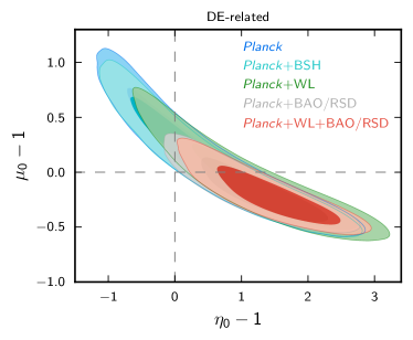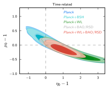Table 6 shows results for the DE-related case for different combinations of the data. Adding the BSH data sets to the Planck TT+lowP data does not significantly increase the constraining power on MG parameters; Planck polarization also has little impact. On the contrary, the addition of RSD data tightens the constraints significantly. The WL contours, including the ultraconservative cut that removes dependence on nonlinear physics, result in weaker constraints. In the table, $\mu_{0}-1$ and $\eta_{0}-1$ are obtained by reconstructing Eqs. (46) and (47) from $E_{11}$ and $E_{22}$ at the present time. In addition, the present value of the $\Sigma$ parameter, defined in Eq. (5), can be obtained from $\mu$ and $\eta$ as $\Sigma=(\mu/2)(1+\eta)$ using Eqs. (4) and (6).

Figure 15: Marginalized posterior distributions for 68% and 95% C.L. for the two parameters $\{\mu_{0}-1,\Sigma_{0}-1\}$ obtained by evaluating Eqs. (46) and (47) at the present time in the DE-related parametrization when no scale dependence is considered (see Sect. 5.2.2). $\Sigma$ is obtained as $\Sigma=(\mu/2)(1+\eta)$. The time-related evolution would give similar contours. In the labels, Planck stands for Planck TT+lowP.

Figure 16: Redshift dependence of the function $2[\mu(z,k)-1]+[\eta(z,k)-1]$, defined in Eqs. (46,47), which corresponds to the maximum degeneracy line identified within the 2 dimensional posterior distributions. This combination shows the strongest allowed tension with $\rm{\Lambda CDM}$. The left panel refers to the DE-related case while the right panel refers to the time-related evolution (see Sect. 5.2.2). In both panels, no scale dependence is considered. The coloured areas show the regions containing 68 % and 95 % of the models. In the labels, Planck stands for Planck TT+lowP.

Figure 17: 68 % and 95 % marginalised posterior distributions for the two parameters $\{\mu_{0}-1,\eta_{0}-1\}$ obtained by evaluating Eqs. (46) and (47) at the present time when no scale dependence is considered (see Sect. 5.2.2). Here we show the effect of CMB lensing, which shifts the contours towards $\rm{\Lambda CDM}$. In the labels, Planck stands for Planck TT+lowP.

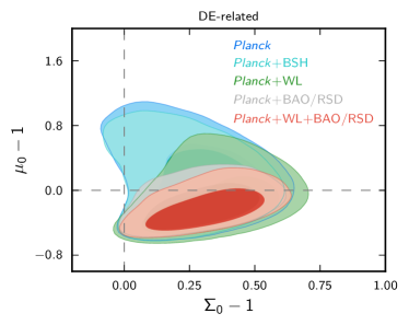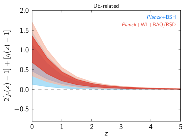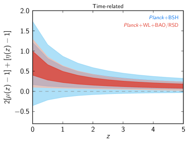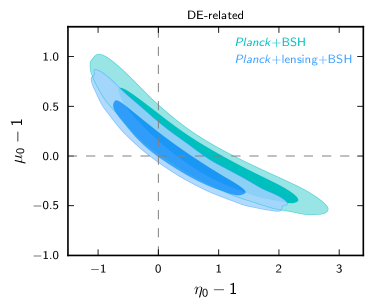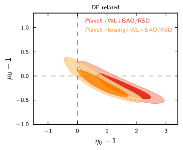Some tension appears, in particular, when plotting the marginalized posterior distributions in the planes ($\mu_{0}-1$, $\eta_{0}-1$) and ($\mu_{0}-1$, $\Sigma_{0}-1$), as shown in Figs. 14 and 15. Here the constraints on the two parameters that describe the perturbations in MG are simultaneously taken into account. In Fig. 14, left and right panels refer to the DE-related and time-related parameterizations defined in 5.2.2, respectively, while the dashed lines indicate the values predicted in $\Lambda$CDM. Interestingly, results appear similar in both parameterizations. In the DE-related case (left panel), the $\rm{\Lambda CDM}$ point lies at the border of the $2\sigma$ contour, already when considering Planck TT+lowP alone. More precisely, when looking at the goodness of fit, with respect to the standard $\Lambda$CDM assumption, the MG scenario (which includes two extra parameters $E_{11}$ and $E_{22}$) leads to an improvement of $\Delta\chi^{2}=-6.3$ when using Planck TT+lowP (similarly divided between lowP and TT) and of $\Delta\chi^{2}=-6.4$ when including BSH (with a $\Delta\chi^{2}_{\rm{CMB}}\sim-5.6$ equally divided between TT and lowP). When Planck data (TT+lowP) are combined also with WL data, the tension increases to $\Delta\chi^{2}=-10.6$ (with the CMB still contributing about the same amount, $\Delta\chi^{2}_{\rm CMB}=-6.0$). When considering Planck TT+lowP+BAO/RSD, $\Delta\chi^{2}=-8.1$ with respect to $\Lambda$CDM while, when combining both WL and BAO/RSD, the tension is maximal, with $\Delta\chi^{2}=-10.8$ and $\chi^{2}_{\rm CMB}=-6.9$. There is instead less tension for the time-related parameterization, as is visible in the right panel of Fig. 14.

Once the behaviour of the coefficients in the two parameterizations is known, we can use Eq. (46) to reconstruct the evolution of $\mu$ and $\eta$ with scale factor (or redshift, equivalently). In Fig. 16 we choose to show the linear combination $2[\mu(z,k)-1]+[\eta(z,k)-1]$, which corresponds approximately to the maximum degeneracy line in the 2 dimensional $\mu-1,\eta-1$ parameter space, which allows to better visualize the joint constraints on $\mu$ and $\eta$ and their maximal allowed departure from $\Lambda$CDM. As expected, the DE-related dependence forces the combination to be compatible with $\rm{\Lambda CDM}$ in the past, when the DE density is negligible; the time-related parameterization, instead allows for a larger variation in the past.

The tension can be understood by noticing that the best fit power spectrum corresponds to a value of $\mu$ and $\eta$ ($E_{11}=-0.3$, $E_{22}=2.2$ for Planck TT+lowP) close to the thick long dashed line shown in Fig. 1 for demonstration. This model leads to less power in the CMB at large scales and a higher lensing potential, which is slightly preferred by the data points with respect to $\rm{\Lambda CDM}$. This explains also why the MG parameters are somewhat degenerate with the lensing amplitude $A_{\rm L}$ (which is an ‘unphysical’ parameter redefining the lensing amplitude that affects the CMB power spectrum). As discussed in Planck Collaboration XIII (2015) (see for ex. Sect. 5.1.2), $\rm{\Lambda CDM}$ would lead to a value of $A_{L}$ (Calabrese et al. 2008) somewhat larger than 1. When varying it in MG, we find a mean value of $A_{\mathrm{L}}=1.116^{+0.095}_{-0.13}$ which is compatible with $A_{L}=1$ at 1 $\sigma$. The price to pay is the tension with $\rm{\Lambda CDM}$ in MG parameter space, which compensates the need for a higher $A_{L}$ that one would have in $\rm{\Lambda CDM}$. The CMB lensing likelihood extracted from the 4- point function of the Planck maps (Planck Collaboration XV 2015) on the other hand does not prefer a higher lensing potential and agrees well with $\rm{\Lambda CDM}$. For this reason the tension is reduced when we add CMB lensing, as shown in Fig. 17. We also note that constraints for this class of model are sensitive to the estimation of the optical depth $\tau$. Smaller values of $\tau$ tend to shift the results further away from $\rm{\Lambda CDM}$.

In order to have a quick overall estimate of the tension for all cases discussed above, we then show in Table 7 the marginalized mean and $68\%$ CL errors for the linear combination $2[\mu(z,k)-1]+[\eta(z,k)-1]$ that . In the table, we indicate in brackets, for convenience, the ‘tension’ with $\rm{\Lambda CDM}$ for each case. This is the maximum allowed tension, since it is calculated along the maximum degeneracy direction. The DE-related parameterization is more in tension with $\rm{\Lambda CDM}$ than the time-related one. The maximum tension reaches 3 $\sigma$ when including WL and BAO/RSD, being therefore mainly driven by external data sets. The inclusion of CMB lensing shifts results towards $\rm{\Lambda CDM}$, as discussed.

Finally, in general, $\mu$ and $\eta$ depend not only on redshift but also on scale, via the parameters ($c_{i}$, $\lambda$). When marginalizing over them, constraints become weaker, as expected. The comparison with the scale-independent case is shown in Fig. 18 for Planck TT+lowP+BSH and different values of $k$. When allowing for scale dependence, the tension with $\rm{\Lambda CDM}$ is washed out by the weakening of the constraints and the goodness of fit does not improve with respect to the scale independent case.

Figure 18: 68 % and 95 % contour plots for the two parameters $\{\mu_{0}(k)-1,\eta_{0}(k)-1\}$ obtained by evaluating Eqs. (46) and (47) at the present time for the DE-related parameterization (see Sect. 5.2.2). We consider both the scale-independent and scale-dependent cases, choosing $k$ values of $10^{-10}{\rm Mpc}^{-1}$ and $10^{2}{\rm Mpc}^{-1}$.

5.3 Further examples of particular models

Quite generally, DE and MG theories deal with at least one extra degree of freedom that can usually be associated with a scalar field. For ‘standard’ DE theories the scalar field couples minimally to gravity, while in MG theories the field can be seen as the mediator of a fifth force in addition to standard interactions. This happens in scalar-tensor theories (including $f(R)$ cosmologies), massive gravity, and all coupled DE models, both when matter is involved or when neutrino evolution is affected. Interactions and fifth forces are therefore a common characteristic of many proposed models, the difference being whether the interaction is universal (i.e., affecting all species with the same coupling, as in scalar-tensor theories) or is different for each species (as in coupled DE, Wetterich 1995b; Amendola 2000 or growing neutrino models, Fardon et al. 2004; Amendola et al. 2008a). In the following we will test well known examples of particular models within all these classes.

5.3.1 Minimally coupled DE: sound speed and k-essence

In minimally coupled quintessence models, the sound speed is $c_{\rm{s}}^{2}=1$ and DE does not contribute significantly to clustering. However, in so-called “k-essence” models, the kinetic term in the action is generalised to an arbitrary function of $(\nabla\phi)^{2}$ (Armendariz-Picon et al. 2000): the sound speed can then be different from the speed of light and if $c_{\rm{s}}\ll 1$, the DE perturbations can become non-negligible on sub-horizon scales and impact structure formation. To test this scenario we have performed a series of analyses where we allow for a constant equation of state parameter $w$ and a constant speed of sound $c_{\rm{s}}^{2}$ (with a uniform prior in $\log c_{\rm{s}}$). We find that the limits on $w$ do not change from the quintessence case and that there is no significant constraint on the DE speed of sound using current data. This can be understood as follows: on scales larger than the sound horizon and for $w$ close to $-1$, DE perturbations are related to dark matter perturbations through $\Delta_{\rm DE}\simeq(1+w)\Delta_{\rm{m}}/4$ and inside the sound horizon they stop growing because of pressure support (see e.g., Creminelli et al. 2009; Sapone & Kunz 2009). In addition, at early times the DE density is much smaller than the matter density, with $\rho_{\rm DE}/\rho_{\rm{m}}=[(1-\Omega_{\rm{m}})/\Omega_{\rm{m}}]a^{-3w}$. Since the relative DE contribution to the perturbation variable $Q(a,k)$ defined in Eq. (3) scales like $\rho_{\rm DE}\Delta_{\rm DE}/(\rho_{\rm{m}}\Delta_{\rm{m}})$, in k-essence type models the impact of the DE perturbations on the total clustering is small when $1+w\approx 0$. For the DE perturbations in k-essence to be detectable, the sound speed would have had to be very small, and $|1+w|$ relatively large.

5.3.2 Massive gravity and generalized scalar field models

We now give two examples of subclasses of Horndeski models, written in terms of an alternative pair of DE perturbation functions (with respect to $\mu$ and $\eta$ used before, for example), given by the anisotropic stress $\sigma$ and the entropy perturbation $\Gamma$:

$$w\Gamma={\delta p\over\rho}-{dp\over d\rho}\delta\thinspace.$$ (48)

When $\Gamma=0$ the perturbations are adiabatic, that is $\delta p={dp\over d\rho}\delta\rho$.

For this purpose, it is convenient to adopt the ‘equation of state’ approach described in Battye et al. (2015); Soergel et al. (2015). The gauge-invariant quantities $\Gamma$ and $\sigma$ can be specified in terms of the other perturbation variables, namely $\delta\rho$, $\theta$, $h$ and $\eta$ in the scalar sector, and their derivatives.

We then show results for two limiting cases in this formalism, corresponding to Lorentz-violating massive gravity (LVMG) for which ($\sigma\neq 0,\Gamma=0$) and generalized scalar field models (GSF) in which the anisotropic stress is zero ($\sigma=0,\Gamma\neq 0$).

Lorentz-violating massive gravity (LVMG)

If the Lagrangian is ${\cal L}\equiv{\cal L}(g_{\mu\nu})$ (i.e. only written in terms of metric perturbations, as in the EFT action) and one imposes time translation invariance (but not spatial translational invariance), one finds that this corresponds to an extra degree of freedom, $\xi^{i}$, that has a physical interpretation as an elastic medium, or as Lorentz-violating massive gravity (Dubovsky 2004; Rubakov & Tinyakov 2008; Battye & Pearson 2013). In this case, the scalar equations are characterized by $\Gamma=0$ (the model is adiabatic) and a non-vanishing anisotropic stress:

$$\sigma=(w-c^{2}_{\rm s})\left[\frac{\delta}{1+w}-3\eta\right]\thinspace,$$ (49)

including one degree of freedom, the sound speed $c^{2}_{\rm s}$, which can be related equivalently to the shear modulus of the elastic medium or the Lorentz violating mass. Tensor (gravitational wave) equations will also include a mass term. The low sound speed may lead to clustering of the DE fluid, which allows the data to place constraints on $c^{2}_{\rm s}$. But as $w$ approaches $-1$, the DE perturbations are suppressed and the limits on the sound speed weaken. We can take this degeneracy between $1+w$ and $c^{2}_{\rm s}$ into account by using the combination $\lambda_{\rm c}=|1+w|^{\alpha}\log_{10}c_{\rm s}^{2}$ in the MCMC analysis, where $\alpha=0.35$ was chosen to decorrelate $w$ and $\lambda_{\rm c}$. With this, we find Planck TT+lowP+lensing gives lower limit of $\lambda_{\rm c}>-1.6$ at $2\sigma$ and a tighter one when including BAO/RSD and WL, with $\lambda_{\rm c}>-1.3$ at $2\sigma$. For any $w\neq-1$ these limits can be translated into limits on $\log_{10}c_{\rm s}^{2}$ by computing $\lambda_{c}/|1+w|^{\alpha}$. The $\rm{\Lambda CDM}$ limit is however fully compatible with the data, i.e. there is no detection of any deviation from $w=-1$ (and in this limit $c^{2}_{\rm s}$ is unconstrained).

Generalized scalar field models (GSF)

One can allow for generalized scalar fields by considering a Lagrangian ${\cal L}\equiv{\cal L}(\phi,\partial_{\mu}\phi,\partial_{\mu}\partial_{\nu}\phi,g_{\mu\nu},\partial_{\alpha}g_{\mu\nu})$, in which the dependence on the scalar fields is made explicit, imposing full reparameterization invariance ($x^{\mu}\rightarrow x^{\nu}+\xi^{\mu}$), allowing for only linear couplings in $\partial_{\alpha}g_{\mu\nu}$ and second-order field equations. In this case the anisotropic stresses are zero and

$$w\Gamma=(\alpha-w)\left\{\delta-3\beta_{1}{\cal H}(1+w)\theta-{3\beta_{2}{\cal H}(1+w)\over 2k^{2}-6(\dot{\cal H}-{\cal H}^{2})}\dot{h}\right.$$

$$\quad+\left.{3(1-\beta_{2}-\beta_{1}){\cal H}(1+w)\over 6\ddot{\cal H}-18{\cal H}\dot{\cal H}+6{\cal H}^{3}+2k^{2}{\cal H}}\ddot{h}\right\}\thinspace.$$ (50)

This has three extra parameters ($\alpha,\beta_{1},\beta_{2}$), in addition to $w$. If $\beta_{1}=1$ and $\beta_{2}=0$ this becomes the generalized k-essence model. An example of this class of models is “kinetic gravity braiding” (Deffayet et al. 2010) and similar to the non-minimally coupled k-essence discussed via EFT in Sect. 5.2.1. The $\alpha$ parameter in Eq. (50) can be now interpreted as a sound speed, unconstrained as in results above. There are however two additional degrees of freedom, $\beta_{1}$ and $\beta_{2}$. RSD data are able to constrain them, with the addition of Planck lensing and WL making only a minor change to the joint constraints. As in the LVMG case, we use a new basis $\gamma_{i}=|1+w|^{\alpha_{i}}\beta_{i}$ in the MCMC analysis, where $\alpha_{1}=0.2$ and $\alpha_{2}=1$ were chosen to decorrelate $w$ and $\gamma_{i}$. The resulting $2\sigma$ upper limits are $\gamma_{1}<0.67$ and $\gamma_{2}<0.61$ (for $w>-1$), $\gamma_{2}<2.4$ (for $w<-1)$ for the combination of Planck TT+lowP+lensing+BAO/RSD+WL. As for the LVMG case, there is no detection of a deviation from $\rm{\Lambda CDM}$  and for $w=-1$ there are no constraints on $\beta_{1}$ and $\beta_{2}$.

5.3.3 Universal couplings: $f(R)$ cosmologies

A well-investigated class of MG models is constituted by the $f(R)$ theories that modify the Einstein-Hilbert action by substituting the Ricci scalar with a more general function of itself:

$$S=\frac{1}{2\kappa^{2}}\int d^{4}x\sqrt{-g}(R+f(R))+\int d^{4}x\mathcal{L}_{\rm M}(\chi_{i},g_{\mu\nu}),$$ (51)

where $\kappa^{2}=8\pi G$. $f(R)$ cosmologies can be mapped to a subclass of scalar-tensor theories, where the coupling of the scalar field to the matter fields is universal.

For a fixed background, the Friedmann equation provides a second-order differential equation for $f(R(a))$ (see e.g., Song et al. 2007a; Pogosian & Silvestri 2008). One of the initial conditions is usually set by requiring

$$\lim_{R\to\infty}\frac{f(R)}{R}=0,$$ (52)

and the other initial (or boundary condition), usually called $B_{0}$, is the present value of

$$B(z)=\frac{f_{RR}}{1+f_{R}}\frac{H\dot{R}}{\dot{H}-H^{2}}.$$ (53)

Here, $f_{R}$ and $f_{RR}$ are the first and second derivatives of $f(R)$, and a dot means a derivative with respect to conformal time. Higher values of $B_{0}$ suppress power at large scales in the CMB power spectrum, due to a change in the ISW effect. This also changes the CMB lensing potential, resulting in slightly smoother peaks at higher $\ell$s (Song et al. 2007b; Schmidt 2008; Bertschinger & Zukin 2008; Marchini et al. 2013).

It is possible to restrict EFTcamb to describe $f(R)$-cosmologies. Given an evolution history for the scale factor and the value of $B_{0}$, EFTcamb effectively solves the Friedmann equation for $f(R)$. It then uses this function at the perturbation level to evolve the metric potentials and matter fields. The merit of EFTcamb over the other available similar codes is that it checks the model against some stability criteria and does not assume the quasi-static regime, where the scales of interest are still linear but smaller than the horizon and the time derivatives are ignored.

As shown in Fig. 19, there is a degeneracy between the optical depth, $\tau$, and the $f(R)$ parameter, $B_{0}$. Adding any structure formation probe, such as WL, RSD or CMB lensing, breaks the degeneracy. Figure 20 shows the likelihood of the $B_{0}$ parameter using EFTcamb, where a $\Lambda$CDM background evolution is assumed, i.e., $w_{\rm DE}=-1$.

As the different data sets provide constraints on $B_{0}$ that vary by more than four orders of magnitude, we show plots for $\log_{10}B_{0}$; to make these figures we use a uniform prior in $\log_{10}B_{0}$ to avoid distorting the posterior due to prior effects. However, for the limits quoted in the tables we use $B_{0}$ (without $\log$) as the fundamental quantity and quote $95\thinspace\%$ limits based on $B_{0}$. In this way the upper limit on $B_{0}$ is effectively given by the location of the drop in probability visible in the figures, but not influenced by the choice of a lower limit of $\log_{10}B_{0}$. Overall this appears to be the best compromise to present the constraints on the $B_{0}$ parameter. In the plots, the GR value ($B_{0}=0$) is reached by a plateau stretching towards minus infinity.

Figure 19: $68\thinspace\%$ and $95\thinspace\%$ contour plots for the two parameters, $\{\rm{Log}_{10}(B_{0}),\tau\}$ (see Sect. 5.3.3). There is a degeneracy between the two parameters for Planck TT+lowP+BSH. Adding lensing will break the degeneracy between the two. Here Planck indicates Planck TT+lowP.

Figure 20: Likelihood plots of the $f(R)$ theory parameter, $B_{0}$ (see Sect. 5.3.3). CMB lensing breaks the degeneracy between $B_{0}$ and the optical depth, $\tau$, resulting in lower upper bounds.

Table 8: $95\thinspace\%$ CL intervals for the $f(R)$ parameter, $B_{0}$ (see Sect. 5.3.3). While the plots are produced for $\log_{10}B_{0}$, the numbers in this table are produced via an analysis on $B_{0}$ since the GR best fit value ($B_{0}=0$) lies out of the bounds in a $\log_{10}B_{0}$ analysis and its estimate would be prior dependent.

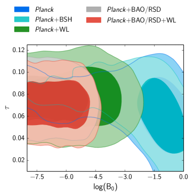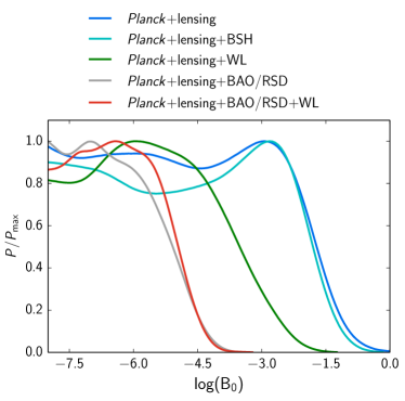Finally, we note that $f(R)$ models can be studied also with the MGcamb parametrization, assuming the quasi-static limit. We find that for the allowed range of the $B_{0}$ parameter, the results with and without the quasi-static approximation are the same within the uncertainties. The $95\thinspace\%$ confidence intervals are reported in Table 8. These values show an improvement over the WMAP analysis made with MGcamb  ($B_{0}<1$ ($95\thinspace\%$ C.L.) in Song et al. (2007a)) and are similar to the limits obtained in Marchini & Salvatelli (2013); Hu et al. (2013) (see also Dossett et al. (2014) where data from WiggleZ were used, Cataneo et al. (2015) where they considered galaxy clusters).

5.3.4 Non-universal couplings: coupled Dark Energy

Universal couplings discussed in the previous subsection generally require screening mechanisms to protect baryonic interactions in high density environments, where local measurements are tightly constraining (see e.g. Khoury 2010 and Vikram et al. (2014) for astrophysical constraints). An alternative way to protect baryons is to allow for non-universal couplings, in which different species can interact with different strengths: baryons are assumed to be minimally coupled to gravity while other species (e.g., dark matter or neutrinos) may feel a “fifth force,” with a range at cosmological scales.

A fifth force between dark matter particles, mediated by the DE scalar field, is the key ingredient for the coupled DE scenario Amendola (2000). In the Einstein frame, the interaction is described by the Lagrangian

$${\cal L}=-\frac{1}{2}\partial^{\mu}\phi\partial_{\mu}\phi-V(\phi)-m(\phi)\bar{\psi}\psi+{\cal L}_{\rm kin}[\psi]\thinspace,$$ (54)

in which the mass of matter fields $\psi$ is not a constant (as in the standard cosmological model), but rather a function of the DE scalar field $\phi$. A coupling between matter and DE can be reformulated in terms of scalar-tensor theories or $f(R)$ models (Wetterich 1995b; Pettorino & Baccigalupi 2008; Wetterich 2014) via a Weyl scaling from the Einstein frame (where matter is coupled and gravity is standard) to the Jordan frame (where the gravitational coupling to the Ricci scalar is modified and matter is uncoupled). This is exactly true when the contribution of baryons is neglected.

Dark matter (indicated with the subscript c) and DE densities are then not conserved separately, but coupled to each other:

$$\rho_{\phi}^{\prime} = -3{\cal{H}}\rho_{\phi}(1+w_{\phi})+{\beta}\rho_{\rm{c}}\phi^{\prime}\thinspace,$$ (55)

$$\rho_{\rm{c}}^{\prime} = -3{\cal{H}}\rho_{\rm{c}}-{\beta}\rho_{\rm{c}}\phi^{\prime}\thinspace.$$

Here each component is treated as a fluid with stress energy tensor ${T^{\nu}}_{(\alpha)\mu}=(\rho_{\alpha}+p_{\alpha})u_{\mu}u^{\nu}+p_{\alpha}\delta^{\nu}_{\mu}$, where $u_{\mu}=(-a,0,0,0)$ is the fluid 4-velocity and $w_{\alpha}\equiv p_{\alpha}/\rho_{\alpha}$ is the equation of state. Primes denote derivatives with respect to conformal time and $\beta$ is assumed, for simplicity, to be a constant. This choice corresponds to a Lagrangian in which dark matter fields have an exponential mass dependence $m(\phi)=m_{0}\exp^{-\beta{\phi}}$ (originally motivated by Weyl scaling scalar-tensor theories), where $m_{0}$ is a constant. The DE scalar field (expressed in units of the reduced Planck mass $M=(8\pi G_{N})^{-1/2}$) evolves according to the Klein-Gordon equation, which now includes an extra term that depends on the density of cold dark matter:

$$\phi^{\prime\prime}+2{\cal H}\phi^{\prime}+a^{2}\frac{dV}{d\phi}=a^{2}\beta\rho_{\rm{c}}\thinspace.$$ (56)

Following Pettorino & Baccigalupi (2008), we choose an inverse power-law potential defined as $V=V_{0}\phi^{-\alpha}$, with $\alpha$ and $V_{0}$ being constants. The amplitude $V_{0}$ is fixed thanks to an iterative routine, as implemented by Amendola et al. (2012b); Pettorino et al. (2012). To a first approximation $\alpha$ only affects late-time cosmology. For numerical reasons, the iterative routine finds the initial value of the scalar field, in the range $\alpha\geq 0.03$, which is close to the $\Lambda$CDM value $\alpha=0$ and extends the range of validity with respect to past attempts; the equation of state $w$ is approximately related to $\alpha$ via the expression (Amendola et al. 2012b): $w=-2/(\alpha+2)$ so that a value of $\alpha=0.03$ corresponds approximately to $w(\alpha=0.03)=-0.99$. The equation of state $w\equiv p/\rho$ is not an independent parameter within coupled DE theories, being degenerate with the flatness of the potential. Dark matter particles then feel a fifth force with an effective gravitational constant $G_{\rm eff}$ that is stronger than the Newtonian one by a factor of $\beta^{2}$, i.e.

$$G_{\rm eff}=G(1+2\beta^{2})\thinspace,$$ (57)

so that a value of $\beta=0$ recovers the standard gravitational interaction. The coupling affects the dynamics of the gravitational potential (and therefore the late ISW effect), hence the shape and amplitude of perturbation growth, and shifts the position of the acoustic peaks to larger multipoles, due to an increase in the distance to the last-scattering surface; furthermore, it reduces the ratio of baryons to dark matter at early times with respect to its present value, since coupled dark matter dilutes faster than in an uncoupled model. The strength of the coupling is known to be degenerate with a combination of $\Omega_{\rm c}$, $n_{\rm s}$ and $H(z)$ (Amendola & Quercellini 2003; Pettorino & Baccigalupi 2008; Bean et al. 2008; Amendola et al. 2012b). Several analyses have previously been carried out, with hints of coupling different from zero, e.g., by Pettorino (2013), who found $\beta=0.036\pm 0.016$ (using Planck 2013 + WMAP polarization + BAO) different from zero at 2.2$\thinspace\sigma$ (the significance increasing to 3.6$\thinspace\sigma$ when data from HST were included).

The marginalized posterior distribution, using Planck 2015 data, for the coupling parameter $\beta$ is shown in Fig. 21, while the corresponding mean values are shown in Table 9. Planck TT data alone gives constraints compatible with zero coupling and the slope of the potential is consistent with a cosmological constant value of $\alpha=0$ at 1.3$\thinspace\sigma$. When other data sets are added, however, both the value of the coupling and the slope of the potential are pushed to non-zero values, i.e., further from $\rm{\Lambda CDM}$. In particular, Planck+BSH gives a value which is $\sim 2.5\thinspace\sigma$ in tension with $\rm{\Lambda CDM}$, while, separately, Planck+WL+BAO/RSD gives a value of the coupling $\beta$ compatible with the one from Planck+BSH and about 2.3$\thinspace\sigma$ away from $\rm{\Lambda CDM}$.

When comparing with $\rm{\Lambda CDM}$, however, the goodness of fit does not improve, despite the additional parameters. Only the $\chi^{2}_{BAO/RSD}$ improves by $\approx 1$ in CDE with respect to $\rm{\Lambda CDM}$, the difference not being significant enough to justify the additional parameters. The fact that the marginalized likelihood does not improve, despite the apparent 2$\thinspace\sigma$ tension, may hint at some dependence on priors: for example, the first panel in Fig. 22 shows that there is some degeneracy between the coupling $\beta$ and the potential slope $\alpha$; while contours are almost compatible with $\rm{\Lambda CDM}$ in the 2 dimensional plot, the marginalization over $\alpha$ takes more contributions from higher values of $\beta$, due to the degeneracy, and seems to give a slight more significant peak in the one dimensional posterior distribution shown in Fig. 21. Whether other priors also contribute to the peak remains to be understood. In any case, the goodness of fit does not point towards a preference for non-zero coupling. Degeneracy between the coupling and other cosmological parameters is shown in the other panels of the same figure, with results compatible with those discussed in Amendola et al. (2012b) and Pettorino (2013). Looking at the conservation equations (i.e., Eqs. 55 and 5.3.4), larger positive values of $\beta$ correspond to a larger transfer of energy from dark matter to DE (effectively adding more DE in the recent past, with roughly $\Omega_{\phi}\propto\beta^{2}$ for an inverse power-law potential) and therefore lead to a smaller $\Omega_{\rm m}$ today; as a consequence, the distance to the last-scattering surface and the expansion rate are modified, with $H^{\prime}/H=-3/2(1+w_{\rm eff})$, where $w_{\rm eff}$ is the effective equation of state given by the ratio of the total pressure over total (weighted) energy density of the coupled fluid; a larger coupling prefers larger $H_{0}$ and higher $\sigma_{8}$.

The addition of polarization tightens the bounds on the coupling, increasing the tension with $\rm{\Lambda CDM}$, reaching $2.8\thinspace\sigma$ and $2.7\thinspace\sigma$ for Planck+BSH and Planck+WL+BAO/RSD, respectively. Also in this case the overall $\chi^{2}$ does not improve between coupled DE and $\rm{\Lambda CDM}$.

Table 9: Marginalized mean values and $68\thinspace\%$ C.L. intervals for coupled DE (see Sect. 5.3.4). Planck here refers to Planck TT+lowP. Results and goodness of fits are discussed in the text. CMB lensing does not improve the constraints significantly.

Figure 21: Marginalized posterior distribution for the coupling $\beta$ (see Sect. 5.3.4). The value corresponding to standard gravity is zero. Results and goodness of fit are discussed in the text.

Figure 22: Marginalized posterior distribution for coupled DE and different combinations of the data sets (see Sect. 5.3.4). Here Planck refers to Planck TT+lowP. We show the degeneracy of the coupling $\beta$ with $\alpha$, $\Omega_{\rm m}$, $\sigma_{8}$ and $H_{0}$.

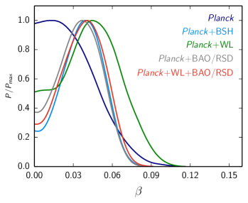6 Conclusions

The quest for Dark Energy and Modified Gravity is far from over. A variety of different theoretical scenarios have been proposed in literature and need to be carefully compared with the data. This effort is still in its early stages, given the variety of theories and parameterizations that have been suggested, together with a lack of well tested numerical codes that allow us to make detailed predictions for the desired range of parameters. In this paper, we have provided a systematic analysis covering a general survey of a variety of theoretical models, including the use of different numerical codes and observational data sets. Even though most of the weight in the Planck data lies at high redshift, Planck can still provide tight constraints on DE and MG, especially when used in combination with other probes. Our focus has been on the scales where linear theory is applicable, since these are the most theoretically robust. Overall, the constraints that we find are consistent with the simplest scenario, $\Lambda$CDM, with constraints on DE models (including minimally-coupled scalar field models or evolving equation of state models) and MG models (including effective field theory, phenomenological parameterizations, $f(R)$ and coupled DE models) that are significantly improved with respect to past analyses. We discuss here our main results, drawing our conclusions for each of them and summarizing the story-line we have followed in this paper to discuss DE and MG.

Our journey started from distinguishing background and perturbation parameterizations. In the first case, the background is modified (which in turn affects the perturbations), leading to the following results.

1. The equation of state $w(z)$ as a function of redshift has been tested for a variety of parameterizations.

   1. In ($w_{0},w_{\rm{a}}$), Planck TT+lowP+BSH is compatible with $\Lambda$CDM, as well as BAO/RSD. When adding WL to Planck TT+lowP, both WL and CMB prefer the ($w_{0},w_{\rm{a}}$) model with respect to $\rm{\Lambda CDM}$ at about $2\sigma$, although with a preference for high values of $H_{0}$ (third panel of Fig. 3) that are excluded when including BSH.

   2. We have reconstructed the equation of state in redshift, testing a Taylor expansion up to the third order in the scale factor and by doing a Principal Component Analysis of $w(z)$ in different redshifts bins. In addition, we have tested an alternative parametrization, that allows to have a varying $w(z)$ that depends on one parameter only. All tests on time varying $w(z)$ are compatible with $\rm{\Lambda CDM}$ for all data sets tested.

2. ‘Background’ Dark Energy models are generally of quintessence type where a scalar field rolls down a potential. We have shown via the ($\epsilon_{\rm{s}},\epsilon_{\rm{\infty}}$) parameterization, related respectively to late and early time evolution, that the quintessence/phantom potential at low redshift must be relatively flat: $d\ln V/d\phi<0.35/M_{\rm P}$ for quintessence; and $d\ln V/d\phi<0.68/M_{\rm P}$ for phantom models. A zero slope ($\Lambda$CDM) remains consistent with the data and compared to previous studies, the uncertainty has been reduced by about 10 %. We have produced a new plot (Fig. 9) that helps to visualize minimally coupled scalar field models, similarly to analogous plots often used in inflationary theories.

3. Information on DE, complementary to ($w_{0},w_{\rm{a}}$), comes from asking whether there can be any DE at early times. First, we have obtained constraints on early DE parametrizations, assuming a constant DE relative density at all epochs until it matches $\rm{\Lambda CDM}$ in recent times: we have improved previous constraints by a factor $\sim 3-4$, leading to $\Omega_{\rm{e}}<0.0071$ at $95\%$ C.L. from Planck TT+lowP+lensing+BSH and $\Omega_{\rm{e}}<0.0036$ for Planck TT,TE,EE+lowP+BSH. In addition, we have also asked how much such tight constraints are weakened when the fraction of early DE is only present in a limited range in redshift and presented a plot of $\Omega_{\rm{e}}(z)$ as a function of $z_{\rm{e}}$, the redshift starting from which a fraction $\Omega_{\rm{e}}$ is present. Also in this case constraints are very tight, with $\Omega_{\rm{e}}\la 2\thinspace\%\thinspace\thinspace(95\thinspace\%$ C.L.) even for $z_{\rm{e}}$ as late as $\approx 50$.

The background is then forced to be very close to $\rm{\Lambda CDM}$, unless the tight constraints on early DE can somehow be evaded in a realistic model by counter balancing effects.

In the second part of the paper, we then moved on to understanding what Planck can say when the evolution of the perturbations is modified independently of the background, as is the case in most MG models. For that, we followed two complementary approaches: one (top-down) that starts from a very general EFT action for DE (Sect. 5.2.1); the other (bottom-up) that starts from parameterizing directly observables (Sect. 5.2.2). In both cases we have assumed that the background is exactly $\rm{\Lambda CDM}$, in order to disentangle the effect of perturbations. We summarize here our results.

1. Starting from EFT theories for DE, which include (almost) all universally coupled models in MG via nine generic functions of time, we have discussed how to restrict them to Horndeski theories, described in terms of five free functions of time. Using the publicly available code EFTcamb, we have then varied three of these functions (in the limits allowed by the code) which correspond to a non-minimally coupled K-essence model (i.e. $\alpha_{\mathrm{B}}$, $\alpha_{\mathrm{M}}$, $\alpha_{\mathrm{K}}$ are varying functions of the scale factor). We have found limits on the present value ${\alpha_{\mathrm{M}}}_{0}<0.052$ at $95\%$ C.L. (in the linear EFT approximation), in agreement with $\rm{\Lambda CDM}$. Constraints depend on the stability routines included in the code, which will need to be further tested in the future, together with allowing for a larger set of choices for the Horndeski functions, not available in the present version of the numerical code.

2. When starting from observables, two functions of time and scale are required to describe perturbations completely, in any model. Among the choices available (summarized in Sect. 3.2.2), we choose $\mu(a,k)$ and $\eta(a,k)$ (other observables can be derived from them). In principle, constraints on these functions are dependent on the chosen parameterization, which needs to be fixed. We have tested two different time dependent parameterizations (DE-related and time-related) and both lead to similar results, although the first is slightly more in tension than the other with $\rm{\Lambda CDM}$ (Fig. 14). In this framework, $\Lambda$CDM lies at the $2\sigma$ limit when Planck TT+lowP+BSH is considered, the tension increasing to about $3\sigma$ when adding WL and BAO/RSD to Planck TT+lowP. As discussed in the text, the mild tension with Planck TT+lowP is related to lower power in the TT spectrum and a larger lensing potential in the MG model, with respect to $\rm{\Lambda CDM}$. The inclusion of CMB lensing shifts all contours back to $\rm{\Lambda CDM}$. We have reconstructed the two observables in redshift for both parameterizations, along the maximum degeneracy line (Fig. 16). When scale dependence is also included, constraints become much weaker and the goodness of fit does not improve, indicating that the data do not seem to need the addition of additional scale dependent parameters.

The last part of the paper discusses a selection of particular MG models of interest in literature.

1. We first commented on the simple case of a minimally coupled scalar field in which not only the equation of state is allowed to vary but the sound speed of the DE fluid is not forced to be 1, as it would be in the case of quintessence. Such a scenario corresponds to k-essence type models. As expected, given that the equation of state is very close to the $\rm{\Lambda CDM}$ value, the total impact of DE perturbations on the clustering is small.

2. We adopt an alternative way to parameterize observables (the equation of state approach) in terms of gauge invariant quantities $\Gamma$ and $\sigma$. We have used this approach to investigate Lorentz-breaking massive gravity and generalised scalar fields models, updating previous bounds.

3. As a concrete example of universally coupled theories, we have considered $f(R)$ models, written in terms of $B(z)$, conventionally related to the first and second derivatives of $f(R)$ with respect to R. Results are compatible with $\rm{\Lambda CDM}$. Such theories assume that some screening mechanism is in place, in order to satisfy current bounds on baryonic physics at solar system scales.

4. Alternatively to screening mechanisms, one can assume that the coupling is not universal, such that baryons are still feeling standard gravitational attraction. As an example of this scenario, we have considered the case in which the dark matter evolution is coupled to the DE scalar field, feeling an effective fifth force stronger than gravity by a factor $\beta^{2}$. Constraints on coupled dark energy show a tension with $\rm{\Lambda CDM}$ at the level of about 2.5 $\sigma$, slightly increasing when including polarization. The apparent tension, however, seems to hint at a dependence on priors, partly related to the degeneracy between the coupling and the slope of the background potential (and possibly others not identified here). Future studies will need to identify the source of tension and possibly disentangle background from perturbation effects.

There are several ways in which the analysis can be extended. We have made an effort to (at least start) to put some order in the variety of theoretical frameworks discussed in literature. There are of course scenarios not included in this picture that deserve future attention, such as additional cosmologies within the EFT (and Horndeski) framework, Galileons (see for example Barreira et al. (2014)), other massive gravity models (see de Rham (2014) for a recent review), general violations of Lorentz invariance as a way to modify GR (Audren et al. 2014), non-local gravity (which, for some choices of the action, appears to fit Planck 2013 data sets (Dirian et al. 2014) as well as $\rm{\Lambda CDM}$, although there is no connection to a fundamental theory available at present); models of bigravity (Hassan & Rosen 2012) appear to be affected by instabilities in the gravitational wave sector (Cusin et al. 2014) (see also Akrami et al. (2015)) and are not considered in this paper. In addition to extending the range of theories, which requires new numerical codes, future tests should verify whether all the assumptions (such as stability constraints, as pointed out in the text) in the currently available codes are justified. Further promising input may come from data sets such as WL and BAO/RSD, that allow to tighten considerably constraints on MG models in which perturbations are modified. With the data available at the time of this paper, there seems to be no significant trend (at more than 3 standard deviations) that compensates any possible tension in $\sigma_{8}$ or $H_{0}$ by favouring Modified Gravity; nevertheless, this issue will need to be further investigated in the future. We also anticipate that these constraints will strengthen with future releases of the Planck data, including improved likelihoods for polarization and new likelihoods, not available at the time of this paper, such as ISW, ISW-lensing and $B$-mode polarization, all of which can be used to further test MG scenarios.