Planck 2015 results. XIII. Cosmological parameters
This paper presents cosmological results based on full-mission Planck observations of temperature and polarization anisotropies of the cosmic microwave background (CMB) radiation. Our results are in very good agreement with the 2013 analysis of the Planck nominal-mission temperature data, but with increased precision. The temperature and polarization power spectra are consistent with the standard spatially-flat 6-parameter cosmology with a power-law spectrum of adiabatic scalar perturbations (denoted “base ” in this paper). From the Planck temperature data combined with Planck lensing, for this cosmology we find a Hubble constant, , a matter density parameter , and a tilted scalar spectral index with , consistent with the 2013 analysis. Note that in this abstract we quote 68 % confidence limits on measured parameters and 95 % upper limits on other parameters. We present the first results of polarization measurements with the Low Frequency Instrument at large angular scales. Combined with the Planck temperature and lensing data, these measurements give a reionization optical depth of , corresponding to a reionization redshift of . These results are consistent with those from WMAP polarization measurements cleaned for dust emission using 353-GHz polarization maps from the High Frequency Instrument. We find no evidence for any departure from base in the neutrino sector of the theory; for example, combining Planck observations with other astrophysical data we find for the effective number of relativistic degrees of freedom, consistent with the value of the Standard Model of particle physics. The sum of neutrino masses is constrained to . The spatial curvature of our Universe is found to be very close to zero, with . Adding a tensor component as a single-parameter extension to base we find an upper limit on the tensor-to-scalar ratio of , consistent with the Planck 2013 results and consistent with the -mode polarization constraints from a joint analysis of BICEP2, Keck Array, and Planck (BKP) data. Adding the BKP -mode data to our analysis leads to a tighter constraint of and disfavours inflationary models with a potential. The addition of Planck polarization data leads to strong constraints on deviations from a purely adiabatic spectrum of fluctuations. We find no evidence for any contribution from isocurvature perturbations or from cosmic defects. Combining Planck data with other astrophysical data, including Type Ia supernovae, the equation of state of dark energy is constrained to , consistent with the expected value for a cosmological constant. The standard big bang nucleosynthesis predictions for the helium and deuterium abundances for the best-fit Planck base cosmology are in excellent agreement with observations. We also analyse constraints on annihilating dark matter and on possible deviations from the standard recombination history. In neither case do we find no evidence for new physics. The Planck results for base are in good agreement with baryon acoustic oscillation data and with the JLA sample of Type Ia supernovae. However, as in the 2013 analysis, the amplitude of the fluctuation spectrum is found to be higher than inferred from some analyses of rich cluster counts and weak gravitational lensing. We show that these tensions cannot easily be resolved with simple modifications of the base cosmology. Apart from these tensions, the base cosmology provides an excellent description of the Planck CMB observations and many other astrophysical data sets.
Key Words.:
Cosmology: observations – Cosmology: theory – cosmic microwave background – cosmological parameters1 Introduction
The cosmic microwave background (CMB) radiation offers an extremely powerful way of testing the origin of fluctuations and of constraining the matter content, geometry, and late-time evolution of the Universe. Following the discovery of anisotropies in the CMB by the COBE satellite (Smoot et al. 1992), ground-based, sub-orbital experiments and notably the WMAP satellite (Bennett et al. 2003, 2013) have mapped the CMB anisotropies with increasingly high precision, providing a wealth of new information on cosmology.
Planck111Planck (http://www.esa.int/Planck) is a project of the European Space Agency (ESA) with instruments provided by two scientific consortia funded by ESA member states and led by Principal Investigators from France and Italy, telescope reflectors provided through a collaboration between ESA and a scientific consortium led and funded by Denmark, and additional contributions from NASA (USA). is the third-generation space mission, following COBE and WMAP, dedicated to measurements of the CMB anisotropies. The first cosmological results from Planck were reported in a series of papers (for an overview see Planck Collaboration I 2014, and references therein) together with a public release of the first 15.5 months of temperature data (which we will refer to as the nominal mission data). Constraints on cosmological parameters from Planck were reported in Planck Collaboration XVI (2014).222This paper refers extensively to the earlier 2013 Planck cosmological parameters paper and CMB power spectra and likelihood paper (Planck Collaboration XVI 2014; Planck Collaboration XV 2014). To simplify the presentation, these papers will henceforth be referred to as PCP13 and PPL13, respectively. The Planck 2013 analysis showed that the temperature power spectrum from Planck was remarkably consistent with a spatially flat cosmology specified by six parameters, which we will refer to as the base model. However, the cosmological parameters of this model were found to be in tension, typically at the 2–3 level, with some other astronomical measurements, most notably direct estimates of the Hubble constant (Riess et al. 2011), the matter density determined from distant supernovae (Conley et al. 2011; Rest et al. 2014), and estimates of the amplitude of the fluctuation spectrum from weak gravitational lensing (Heymans et al. 2013; Mandelbaum et al. 2013) and the abundance of rich clusters of galaxies (Planck Collaboration XX 2014; Benson et al. 2013; Hasselfield et al. 2013). As reported in the revised version of PCP13, and discussed further in Sect. 5, some of these tensions have been resolved with the acquisition of more astrophysical data, while other new tensions have emerged.
The primary goal of this paper is to present the results from the full Planck mission, including a first analysis of the Planck polarization data. In addition, this paper introduces some refinements in data analysis and addresses the effects of small instrumental systematics discovered (or better understood) since PCP13 appeared.
The Planck 2013 data were not entirely free of systematic effects. The Planck instruments and analysis chains are complex and our understanding of systematics has improved since PCP13. The most important of these was the incomplete removal of line-like features in the power spectrum of the time-ordered data, caused by interference of the 4-K cooler electronics with the bolometer readout electronics. This resulted in correlated systematics across detectors, leading to a small “dip” in the power spectra at multipoles at 217 GHz, which is most noticeable in the first sky survey. Various tests were presented in PCP13 that suggested that this systematic caused only small shifts to cosmological parameters. Further analyses, based on the full mission data from the HFI (29 months, 4.8 sky surveys) are consistent with this conclusion (see Sect. 3). In addition, we discovered a minor error in the beam transfer functions applied to the 2013 217-GHz spectra, which had negligible impact on the scientific results. Another feature of the Planck data, not fully understood at the time of the 2013 data release, was a calibration offset (in power) between Planck and WMAP (reported in PCP13, see also Planck Collaboration XXXI 2014). As discussed in Appendix A of PCP13, the 2013 Planck and WMAP power spectra agree to high precision if this multiplicative factor is taken into account and it has no significant impact on cosmological parameters apart from a rescaling of the amplitude of the primordial fluctuation spectrum. The reasons for the 2013 calibration offsets are now largely understood and in the 2015 release the calibrations of both Planck instruments and WMAP are consistent to within about in power (see Planck Collaboration I 2016, for further details). In addition, the Planck beams have been characterized more accurately in the 2015 data release and there have been minor modifications to the low-level data processing.
The layout of this paper is as follows. Section 2 summarizes a number of small changes to the parameter estimation methodology since PCP13. The full mission temperature and polarization power spectra are presented in Sect. 3. The first subsection (Sect. 3.1) discusses the changes in the cosmological parameters of the base cosmology compared to those presented in 2013. Section 3.2 presents an assessment of the impact of foreground cleaning (using the 545-GHz maps) on the cosmological parameters of the base model. The power spectra and associated likelihoods are presented in Sect. 3.3. This subsection also discusses the internal consistency of the Planck , , and spectra. The agreement of and with the spectra provides an important additional test of the accuracy of our foreground corrections to the spectra at high multipoles.
PCP13 used the WMAP polarization likelihood at low multipoles to constrain the reionization optical depth parameter . The 2015 analysis replaces the WMAP likelihood with polarization data from the Planck Low Frequency Instrument (LFI, Planck Collaboration II 2016). The impact of this change on is discussed in Sect. 3.4, which also presents an alternative (and competitive) constraint on based on combining the Planck spectrum with the power spectrum of the lensing potential measured by Planck. We also compare the LFI polarization constraints with the WMAP polarization data cleaned with the Planck HFI 353-GHz maps.
Section 4 compares the Planck power spectra with the power spectra from high-resolution ground-based CMB data from the Atacama Cosmology Telescope (ACT, Das et al. 2014) and the South Pole Telescope (SPT, George et al. 2015). This section applies a Gibbs sampling technique to sample over foreground and other “nuisance” parameters to recover the underlying CMB power spectrum at high multipoles (Dunkley et al. 2013; Calabrese et al. 2013). Unlike PCP13, in which we combined the likelihoods of the high-resolution experiments with the Planck temperature likelihood, in this paper we use the high-resolution experiments mainly to check the consistency of the “damping tail” in the Planck power spectrum at multipoles .
Section 5 introduces additional data, including the Planck lensing likelihood (described in detail in Planck Collaboration XV 2016) and other astrophysical data sets. As in PCP13, we are highly selective in the astrophysical data sets that we combine with Planck. As mentioned above, the main purpose of this paper is to describe what the Planck data have to say about cosmology. It is not our purpose to present an exhaustive discussion of what happens when the Planck data are combined with a wide range of astrophysical data. This can be done by others, using the publicly released Planck likelihood. Nevertheless, some cosmological parameter combinations are highly degenerate using CMB power spectrum measurements alone, the most severe being the “geometrical degeneracy” that opens up when spatial curvature is allowed to vary. Baryon acoustic oscillation (BAO) measurements are a particularly important astrophysical data set. Since BAO surveys involve a simple geometrical measurement, these data are less prone to systematic errors than most other astrophysical data. As in PCP13, BAO measurements are used as a primary astrophysical data set in combination with Planck to break parameter degeneracies. It is worth mentioning explicitly our approach to interpreting tensions between Planck and other astrophysical data sets. Tensions may be indicators of new physics beyond that assumed in the base model. However, they may also be caused by systematic errors in the data. Our primary goal is to report whether the Planck data support any evidence for new physics. If evidence for new physics is driven primarily by astrophysical data, but not by Planck, then the emphasis must necessarily shift to establishing whether the astrophysical data are free of systematics. This type of assessment is beyond the scope of this paper, but sets a course for future research.
Extensions to the base cosmology are discussed in Sect. 6, which explores a large grid of possibilities. In addition to these models, we also explore constraints on big bang nucleosynthesis, dark matter annihilation, cosmic defects, and departures from the standard recombination history. As in PCP13, we find no convincing evidence for a departure from the base model. As far as we can tell, a simple inflationary model with a slightly tilted, purely adiabatic, scalar fluctuation spectrum fits the Planck data and most other precision astrophysical data. There are some “anomalies” in this picture, including the poor fit to the CMB temperature fluctuation spectrum at low multipoles, as reported by WMAP (Bennett et al. 2003) and in PCP13, suggestions of departures from statistical isotropy at low multipoles (as reviewed in Planck Collaboration XXIII 2014; Planck Collaboration XVI 2016), and hints of a discrepancy with the amplitude of the matter fluctuation spectrum at low redshifts (see Sect. 5.5). However, none of these anomalies are of decisive statistical significance at this stage.
One of the most interesting developments since the appearance of PCP13 was the detection by the BICEP2 team of a -mode polarization anisotropy (BICEP2 Collaboration 2014), apparently in conflict with the 95 % upper limit on the tensor-to-scalar ratio, ,333The subscript on refers to the pivot scale in used to define the tensor-to-scalar ratio. For Planck we usually quote , since a pivot scale of is close to the scale at which there is some sensitivity to tensor modes in the large-angle temperature power spectrum. For a scalar spectrum with no running and a scalar spectral index of , for small . For , assuming the inflationary consistency relation, we have instead . reported in PCP13. Clearly, the detection of -mode signal from primordial gravitational waves would have profound consequences for cosmology and inflationary theory. However, a number of studies, in particular an analysis of Planck 353-GHz polarization data, suggested that polarized dust emission might contribute a significant part of the BICEP2 signal (Planck Collaboration Int. XXX 2016; Mortonson & Seljak 2014; Flauger et al. 2014). The situation is now clearer following the joint analysis of BICEP2, Keck Array, and Planck data (BICEP2/Keck Array and Planck Collaborations 2015, hereafter BKP); this increases the signal-to-noise ratio on polarized dust emission primarily by directly cross-correlating the BICEP2 and Keck Array data at 150 GHz with the Planck polarization data at 353 GHz. The results of BKP give a 95 % upper limit on the tensor-to-scalar ratio of , with no statistically significant evidence for a primordial gravitational wave signal. Section 6.2 presents a brief discussion of this result and how it fits in with the indirect constraints on derived from the Planck 2015 data.
Our conclusions are summarized in Sect. 7.
2 Model, parameters, and methodology
The notation, definitions and methodology used in this paper largely follow those described in PCP13, and so will not be repeated here. For completeness, we list some derived parameters of interest in Sect. 2.2. We have made a small number of modifications to the methodology, as described in Sect. 2.1. We have also made some minor changes to the model of unresolved foregrounds and nuisance parameters used in the high- likelihood. These are described in detail in Planck Collaboration XI (2016), but to make this paper more self-contained, these changes are summarized in Sect. 2.3.
2.1 Theoretical model
We adopt the same general methodology as described in PCP13, with small modifications. Our main results are now based on the lensed CMB power spectra computed with the updated January 2015 version of the camb444http://camb.info Boltzmann code (Lewis et al. 2000), and parameter constraints are based on the January 2015 version of CosmoMC (Lewis & Bridle 2002; Lewis 2013). Changes in our physical modelling are as follows.
-
For each model in which the fraction of baryonic mass in helium is not varied independently of other parameters, it is now set from the big bang nucleosynthesis (BBN) prediction by interpolation from a recent fitting formula based on results from the PArthENoPE BBN code (Pisanti et al. 2008). We now use a fixed fiducial neutron decay constant of , and also account for the small difference between the mass-fraction ratio and the nucleon-based fraction . These modifications result in changes of about 1 % to the inferred value of compared to PCP13, giving best-fit values () in . See Sect. 6.5 for a detailed discussion of the impact of uncertainties arising from variations of and nuclear reaction rates; however, these uncertainties have minimal impact on our main results. Section 6.5 also corrects a small error arising from how the difference between and was handled in the BBN fitting formula.
-
We have corrected a missing source term in the dark energy modelling for . The correction of this error has very little impact on our science results, since it is only important for values of far from .
-
To model the small-scale matter power spectrum, we use the halofit approach (Smith et al. 2003), with the updates of Takahashi et al. (2012), as in PCP13, but with revised fitting parameters for massive neutrino models.555Results for neutrino models with galaxy and CMB lensing alone use the camb Jan 2015 version of halofit to avoid problems at large ; other results use the previous (April 2014) halofit version. We also now include the halofit corrections when calculating the lensed CMB power spectra.
As in PCP13 we adopt a Bayesian framework for testing theoretical models. Tests using the “profile likelihood” method, described in Planck Collaboration Int. XVI (2014), show excellent agreement for the mean values of the cosmological parameters and their errors, for both the base model and its extension. Tests have also been carried out using the class Boltzmann code (Lesgourgues 2011) and the Monte Python MCMC code (Audren et al. 2013) in place of camb and CosmoMC, respectively. Again, for flat models we find excellent agreement with the baseline choices used in this paper.
2.2 Derived parameters
Our base parameters are defined as in PCP13, and we also calculate the same derived parameters. In addition we now compute:
-
the helium nucleon fraction defined by ;
-
where standard BBN is assumed, the mid-value deuterium ratio predicted by BBN, , using a fit from the PArthENoPE BBN code (Pisanti et al. 2008);
-
the comoving wavenumber of the perturbation mode that entered the Hubble radius at matter-radiation equality , where this redshift is calculated approximating all neutrinos as relativistic at that time, i.e., ;
-
the comoving angular diameter distance to last scattering, ;
-
the angular scale of the sound horizon at matter-radiation equality, , where is the sound horizon and is the redshift of last scattering;
-
the amplitude of the CMB power spectrum in K2, for , 220, 810, 1520, and 2000;
-
the primordial spectral index of the curvature perturbations at wavenumber , (as in PCP13, our default pivot scale is , so that );
-
parameter combinations close to those probed by galaxy and CMB lensing (and other external data), specifically and ;
2.3 Changes to the foreground model
Unresolved foregrounds contribute to the temperature power spectrum and must be modelled to extract accurate cosmological parameters. PPL13 and PCP13 used a parametric approach to modelling foregrounds, similar to the approach adopted in the analysis of the SPT and ACT experiments (Reichardt et al. 2012; Dunkley et al. 2013). The unresolved foregrounds are described by a set of power spectrum templates together with nuisance parameters, which are sampled via MCMC along with the cosmological parameters.666Our treatment of Galactic dust emission also differs from that used in PPL13 and PCP13. Here we describe changes to the extragalactic model and our treatment of errors in the Planck absolute calibration, deferring a discussion of Galactic dust modelling in temperature and polarization to Sect. 3. The components of the extragalactic foreground model consist of:
-
the shot noise from Poisson fluctuations in the number density of point sources;
-
the power due to clustering of point sources (loosely referred to as the CIB component);
-
a thermal Sunyaev-Zeldovich (tSZ) component;
-
a kinetic Sunyaev-Zeldovich (kSZ) component;
-
the cross-correlation between tSZ and CIB.
In addition, the likelihood includes a number of other nuisance parameters, such as relative calibrations between frequencies, and beam eigenmode amplitudes. We use the same templates for the tSZ, kSZ, and tSZ/CIB cross-correlation as in the 2013 papers. However, we have made a number of changes to the CIB modelling and the priors adopted for the SZ effects, which we now describe in detail.
2.3.1 CIB
In the 2013 papers, the CIB anisotropies were modelled as a power law:
| (1) |
Planck data alone provide a constraint on and very weak constraints on the CIB amplitudes at lower frequencies. PCP13 reported typical values of and , fitted over the range . The addition of the ACT and SPT data (“highL”) led to solutions with steeper values of , closer to , suggesting that the CIB component was not well fit by a power law.
Planck results on the CIB, using H i as a tracer of Galactic dust, are discussed in detail in Planck Collaboration XXX (2014). In that paper, a model with 1-halo and 2-halo contributions was developed that provides an accurate description of the Planckand IRAS CIB spectra from 217 GHz through to 3000 GHz. At high multipoles, , the halo-model spectra are reasonably well approximated by power laws, with a slope (though see Sect. 4). At multipoles in the range , corresponding to the transition from the 2-halo term dominating the clustering power to the 1-halo term dominating, the Planck Collaboration XXX (2014) templates have a shallower slope, consistent with the results of PCP13. The amplitudes of these templates at are
| (2) |
Note that in PCP13, the CIB amplitude of the spectrum was characterized by a correlation coefficient
| (3) |
The combined Planck+highL solutions in PCP13 always give a high correlation coefficient with a lower limit of , consistent with the model of Eq. (2), which has . In the 2015 analysis, we use the Planck Collaboration XXX (2014) templates, fixing the relative amplitudes at , , and to the amplitude of the spectrum. Thus, the CIB model used in this paper is specified by only one amplitude, , which is assigned a uniform prior in the range 0–200 .
In PCP13 we solved for the CIB amplitudes at the CMB effective frequencies of and GHz, and so we included colour corrections in the amplitudes and (there was no CIB component in the spectrum). In the 2015 Planck analysis, we do not include a colour term since we define to be the actual CIB amplitude measured in the Planck -GHz band. This is higher by a factor of about compared to the amplitude at the CMB effective frequency of the Planck 217-GHz band. This should be borne in mind by readers comparing and CIB amplitudes measured by Planck.
2.3.2 Thermal and kinetic SZ amplitudes
In the 2013 papers we assumed template shapes for the thermal (tSZ) and kinetic (kSZ) spectra characterized by two amplitudes, and , defined in equations (26) and (27) of PCP13. These amplitudes were assigned uniform priors in the range 0–10 . We used the Trac et al. (2011) kSZ template spectrum and the tSZ template from Efstathiou & Migliaccio (2012). We adopt the same templates for the 2015 Planck analysis, since, for example, the tSZ template is actually a good match to the results from the recent numerical simulations of McCarthy et al. (2014). In addition, we previously included a template from Addison et al. (2012) to model the cross-correlation between the CIB and tSZ emission from clusters of galaxies. The amplitude of this template was characterized by a dimensionless correlation coefficient, , which was assigned a uniform prior in the range 0–1. The three parameters , , and , are not well constrained by Planck alone. Even when combined with ACT and SPT, the three parameters are highly correlated with each other. Marginalizing over , Reichardt et al. (2012) find that SPT spectra constrain the linear combination
| (4) |
The slight differences in the coefficients compared to the formula given in Reichardt et al. (2012) come from the different effective frequencies used to define the Planck amplitudes and . An investigation of the 2013 Planck+highL solutions show a similar degeneracy direction, which is almost independent of cosmology, even for extensions to the base model:
| (5) |
for Planck+WP+highL, which is very close to the degeneracy direction (Eq. 4) measured by SPT. In the 2015 Planck analysis, we impose a conservative Gaussian prior for , as defined in Eq. (5), with a mean of and a dispersion (i.e., somewhat broader than the dispersion measured by Reichardt et al. 2012). The purpose of imposing this prior on is to prevent the parameters and from wandering into unphysical regions of parameter space when using Planck data alone. We retain the uniform prior of [0,1] for . As this paper was being written, results from the complete 2540 SPT-SZ survey area appeared (George et al. 2015). These are consistent with Eq. (5) and in addition constrain the correlation parameter to low values, . The looser priors on these parameters adopted in this paper are, however, sufficient to eliminate any significant sensitivity of cosmological parameters derived from Planck to the modelling of the SZ components.
2.3.3 Absolute Planck calibration
In PCP13, we treated the calibrations of the 100 and 217-GHz channels relative to as nuisance parameters. This was an approximate way of dealing with small differences in relative calibrations between different detectors at high multipoles, caused by bolometer time-transfer function corrections and intermediate and far sidelobes of the Planck beams. In other words, we approximated these effects as a purely multiplicative correction to the power spectra over the multipole range –. The absolute calibration of the 2013 Planck power spectra was therefore fixed, by construction, to the absolute calibration of the 143-5 bolometer. Any error in the absolute calibration of this reference bolometer was not propagated into errors on cosmological parameters. For the 2015 Planck likelihoods we use an identical relative calibration scheme between , , and GHz, but we now include an absolute calibration parameter , at the map level, for the 143-GHz reference frequency. We adopt a Gaussian prior on centred on unity with a (conservative) dispersion of . This overall calibration uncertainty is then propagated through to cosmological parameters such as and . A discussion of the consistency of the absolute calibrations across the nine Planck frequency bands is given in Planck Collaboration I (2016).
3 Constraints on the parameters of the base CDM cosmology from Planck
3.1 Changes in the base parameters compared to the 2013 data release
| [1] Parameter [2] 2013N(DS) [3] 2013F(DS) [4] 2013F(CY) [5] 2015F(CHM) [6] 2015F(CHM) (Plik) . . . . . . . . . |
The principal conclusion of PCP13 was the excellent agreement of the base model with the temperature power spectra measured by Planck. In this subsection, we compare the parameters of the base model reported in PCP13 with those measured from the full-mission 2015 data. Here we restrict the comparison to the high multipole temperature () likelihood (plus low- polarization), postponing a discussion of the and likelihood blocks to Sect. 3.2. The main differences between the 2013 and 2015 analyses are as follows.
(1)
There have been a number of changes to the low-level Planck data processing, as discussed in Planck Collaboration II (2016) and Planck Collaboration VII (2016). These include: changes to the filtering applied to remove “4-K” cooler lines from the time-ordered data (TOD); changes to the deglitching algorithm used to correct the TOD for cosmic ray hits; improved absolute calibration based on the spacecraft orbital dipole and more accurate models of the beams, accounting for the intermediate and far sidelobes. These revisions largely eliminate the calibration difference between Planck-2013 and WMAP reported in PCP13 and Planck Collaboration XXXI (2014), leading to upward shifts of the HFI and LFI Planck power spectra of approximately 2.0 % and 1.7 %, respectively. In addition, the mapmaking used for 2015 data processing utilizes “polarization destriping” for the polarized HFI detectors (Planck Collaboration VIII 2016).
(2)
The 2013 papers used WMAP polarization measurements (Bennett et al. 2013) at multipoles to constrain the optical depth parameter ; this likelihood was denoted “WP” in the 2013 papers. In the 2015 analysis, the WMAP polarization likelihood is replaced by a Planck polarization likelihood constructed from low-resolution maps of and polarization measured by LFI at GHz, foreground cleaned using the LFI 30-GHz and HFI 353-GHz maps as polarized synchrotron and dust templates, respectively, as described in Planck Collaboration XI (2016). After a comprehensive analysis of survey-to-survey null tests, we found possible low-level residual systematics in Surveys 2 and 4, likely related to the unfavourable alignment of the CMB dipole in those two surveys (for details see Planck Collaboration II 2016). We therefore conservatively use only six of the eight LFI 70-GHz full-sky surveys, excluding Surveys 2 and 4, The foreground-cleaned LFI 70-GHz polarization maps are used over 46 % of the sky, together with the temperature map from the Commander component-separation algorithm over 94 % of the sky (see Planck Collaboration IX 2016, for further details), to form a low- Planck temperature+polarization pixel-based likelihood that extends up to multipole . Use of the polarization information in this likelihood is denoted as “lowP” in this paper The optical depth inferred from the lowP likelihood combined with the Planck likelihood is typically , and is about lower than the typical values of inferred from the WMAP polarization likelihood (see Sect. 3.4) used in the 2013 papers. As discussed in Sect. 3.4 (and in more detail in Planck Collaboration XI 2016) the LFI 70-GHz and WMAP polarization maps are consistent when both are cleaned with the HFI 353-GHz polarization maps.777Throughout this paper, we adopt the following labels for likelihoods: (i) Planck TT denotes the combination of the likelihood at multipoles and a low- temperature-only likelihood based on the CMB map recovered with Commander; (ii) Planck TT+lowP further includes the Planck polarization data in the low- likelihood, as described in the main text; (iii) labels such as Planck TE+lowP denote the likelihood at plus the polarization-only component of the map-based low- Planck likelihood; and (iv) Planck TT,TE,EE+lowP denotes the combination of the likelihood at using , , and spectra and the low- temperature+polarization likelihood. We make occasional use of combinations of the polarization likelihoods at and the temperature+polarization data at low-, which we denote with labels such as Planck TE+lowT,P.
(3)
In the 2013 papers, the Planck temperature likelihood was a hybrid: over the multipole range –49, the likelihood was based on the Commander algorithm applied to 87 % of the sky computed using a Blackwell-Rao estimatorl the likelihood at higher multipoles (–2500) was constructed from cross-spectra over the frequency range 100–217 GHz using the CamSpec software (Planck Collaboration XV 2014), which is based on the methodology developed in Efstathiou (2004) and Efstathiou (2006). At each of the Planck HFI frequencies, the sky is observed by a number of detectors. For example, at 217 GHz the sky is observed by four unpolarized spider-web bolometers (SWBs) and eight polarization sensitive bolometers (PSBs). The TOD from the 12 bolometers can be combined to produce a single map at 217 GHz for any given period of time. Thus, we can produce 217-GHz maps for individual sky surveys (denoted S1, S2, S3, etc.), or by year (Y1, Y2), or split by half-mission (HM1, HM2). We can also produce a temperature map from each SWB and a temperature and polarization map from quadruplets of PSBs. For example, at 217 GHz we produce four temperature and two temperature+polarization maps. We refer to these maps as detectors-set maps (or “DetSets” for short); note that the DetSet maps can also be produced for any arbitrary time period. The high multipole likelihood used in the 2013 papers was computed by cross-correlating HFI DetSet maps for the “nominal” Planck mission extending over 15.5 months.888Although we analysed a Planck full-mission temperature likelihood extensively, prior to the release of the 2013 papers. For the 2015 papers we use the full-mission Planck data, extending over 29 months for the HFI and 48 months for the LFI. In the Planck 2015 analysis, we have produced cross-year and cross-half-mission likelihoods in addition to a DetSet likelihood. The baseline 2015 Planck temperature-polarization likelihood is also a hybrid, matching the high-multipole likelihood at to the Planck pixel-based likelihood at lower multipoles.
(4)
The sky coverage used in the CamSpec likelihood was intentionally conservative, retaining effectively 49 % of the sky at 100 GHz and 31 % of the sky at 143 and 217 GHz.999These quantities are explicitly the apodized effective , calculated as the average of the square of the apodized mask values (see Eq. 10). This was done to ensure that on the first exposure of Planck cosmological results to the community, corrections for Galactic dust emission were demonstrably small and had negligible impact on cosmological parameters. In the 2015 analysis we make more aggressive use of the sky at each of these frequencies. We have also tuned the point-source masks to each frequency, rather than using a single point-source mask constructed from the union of the point source catalogues at 100, 143, 217, and 353 GHz. This results in many fewer point source holes in the 2015 analysis compared to the 2013 analysis.
(5)
Most of the results in this paper are derived from a revised Plik likelihood, based on cross-half-mission spectra. The Plik likelihood has been modified since 2013 so that it is now similar to the CamSpec likelihood used in PCP13. Both likelihoods use similar approximations to compute the covariance matrices. The main difference is in the treatment of Galactic dust corrections in the analysis of the polarization spectra. The two likelihoods have been written independently and give similar (but not identical) results, as discussed further below. The Plik likelihood is discussed in Planck Collaboration XI (2016). The CamSpec likelihood is discussed in a separate paper (Efstathiou et al. in preparation).
(6)
We have made minor changes to the foreground modelling and to the priors on some of the foreground parameters, as discussed in Sect. 2.3 and Planck Collaboration XI (2016).
Given these changes to data processing, mission length, sky coverage, etc., it is reasonable to ask whether the base parameters have changed significantly compared to the 2013 numbers. In fact, the parameter shifts are relatively small. The situation is summarized in Table 1. The second column of this table lists the Planck+WP parameters, as given in table 5 of PCP13. Since these numbers are based on the 2013 processing of the nominal mission and computed via a DetSet CamSpec likelihood, the column is labelled 2013N(DS). We now make a number of specific remarks about these comparisons.
(1) 4-K cooler line systematics.
After the submission of PCP13 we found strong evidence that a residual in the DetSet spectrum at was a systematic caused by electromagnetic interference between the Joule-Thomson 4-K cooler electronics and the bolometer readout electronics. This interference leads to a set of time-variable narrow lines in the power spectrum of the TOD. The data processing pipelines apply a filter to remove these lines; however, the filtering failed to reduce their impact on the power spectra to negligible levels. Incomplete removal of the 4-K cooler lines affects primarily the PSBPSB cross-spectrum in Survey 1. The presence of this systematic was reported in the revised versions of 2013 Planck papers. Using simulations and also comparison with the 2013 full-mission likelihood (in which the power spectrum “dip” is strongly diluted by the additional sky surveys) we assessed that the 4-K line systematic was causing shifts in cosmological parameters of less than .101010The revised version of PCP13 also reported an error in the ordering of the beam-transfer functions applied to some of the 2013 DetSet cross-spectra, leading to an offset of a few in the coadded spectrum. As discussed in PCP13, this offset is largely absorbed by the foreground model and has negligible impact on the 2013 cosmological parameters. Column 3 in Table 1 lists the DetSet parameters for the full-mission 2013 data. This full-mission likelihood uses more extensive sky coverage than the nominal mission likelihood (effectively 39 % of sky at 217 GHz, 55 % of sky at 143 GHz, and 63 % of sky at 100 GHz); otherwise the methodology and foreground model are identical to the CamSpec likelihood described in PPL13. The parameter shifts are relatively small and consistent with the improvement in signal-to-noise of the full-mission spectra and the systematic shifts caused by the dip in the nominal mission (for example, raising and , as discussed in appendix C4 of PCP13).
(2) DetSets versus cross-surveys.
In a reanalysis of the publicly released Planck maps, Spergel et al. (2015) constructed cross-survey () likelihoods and found cosmological parameters for the base model that were close to (within approximately ) the nominal mission parameters listed in Table 1. The Spergel et al. (2015) analysis differs substantially in sky coverage and foreground modelling compared to the 2013 Planck analysis and so it is encouraging that they find no major differences with the results presented by the Planck collaboration. On the other hand, they did not identify the reasons for the roughly parameter shifts. They argue that foreground modelling and the dip in the DetSet spectrum can contribute towards some of the differences but cannot produce shifts, in agreement with the conclusions of PCP13. The 2013F(DS) likelihood disfavours the Spergel et al. (2015) cosmology (with parameters listed in their table 3) by , i.e., by about , and almost all of the is contributed by the multipole range 1000–1500, so the parameter shifts are not driven by cotemporal systematics resulting in correlated noise biases at high multipoles. However, as discussed in PPL13 and Planck Collaboration XI (2016), low-level correlated noise in the DetSet spectra affects all HFI channels at high multipoles where the spectra are noise dominated. The impact of this correlated noise on cosmological parameters is relatively small. This is illustrated by column 4 of Table 1 (labelled “2013F(CY)”), which lists the parameters of a 2013 CamSpec cross-year likelihood using the same sky coverage and foreground model as the DetSet likelihood used for column 3. The parameters from these two likelihoods are in good agreement (better than ), illustrating that cotemporal systematics in the DetSets are at sufficiently low levels that there is very little effect on cosmological parameters. Nevertheless, in the 2015 likelihood analysis we apply corrections for correlated noise to the DetSet cross-spectra, as discussed in Planck Collaboration XI (2016), and typically find agreement in cosmological parameters between DetSet, cross-year, and cross-half-mission likelihoods to better than accuracy for a fixed likelihood code (and to better than accuracy for base ).
(3) 2015 versus 2013 processing.
Column 5 (labelled “2015F(CHM)”) lists the parameters computed from the CamSpec cross-half-mission likelihood using the HFI 2015 data with revised absolute calibration and beam-transfer functions. We also replace the WP likelihood of the 2013 analysis with the Planck lowP likelihood. The 2015F(CHM) likelihood uses slightly more sky coverage (60 %) at 217 GHz, compared to the 2013F(CY) likelihood and also uses revised point source masks. Despite these changes, the base parameters derived from the 2015 CamSpec likelihood are within of the 2013F(CY) parameters, with the exception of , which is lower by , , which is lower by , and , which is higher by about . The change in simply reflects the preference for a lower value of from the Planck LFI polarization data compared to the WMAP polarization likelihood in the form delivered by the WMAP team (see Sect. 3.4 for further discussion). The large upward shift in reflects the change in the absolute calibration of the HFI. As noted in Sect. 2.3, the 2013 analysis did not propagate an error on the Planck absolute calibration through to cosmological parameters. Coincidentally, the changes to the absolute calibration compensate for the downward change in and variations in the other cosmological parameters to keep the parameter largely unchanged from the 2013 value. This will be important when we come to discuss possible tensions between the amplitude of the matter fluctuations at low redshift estimated from various astrophysical data sets and the Planck CMB values for the base cosmology (see Sect. 5.6).
(4) Likelihoods.
Constructing a high-multipole likelihood for Planck, particularly with and spectra, is complicated and difficult to check at the sub- level against numerical simulations because the simulations cannot model the foregrounds, noise properties, and low-level data processing of the real Planck data to sufficiently high accuracy. Within the Planck collaboration, we have tested the sensitivity of the results to the likelihood methodology by developing several independent analysis pipelines. Some of these are described in Planck Collaboration XI (2016). The most highly developed of them are the CamSpec and revised Plik pipelines. For the 2015 Planck papers, the Plik pipeline was chosen as the baseline. Column 6 of Table 1 lists the cosmological parameters for base determined from the Plik cross-half-mission likelihood, together with the lowP likelihood, applied to the 2015 full-mission data. The sky coverage used in this likelihood is identical to that used for the CamSpec 2015F(CHM) likelihood. However, the two likelihoods differ in the modelling of instrumental noise, Galactic dust, treatment of relative calibrations, and multipole limits applied to each spectrum.
As summarized in column 8 of Table 1, the Plik and CamSpec parameters agree to within , except for , which differs by nearly . The difference in is perhaps not surprising, since this parameter is sensitive to small differences in the foreground modelling. Differences in between Plik and CamSpec are systematic and persist throughout the grid of extended models discussed in Sect. 6. We emphasize that the CamSpec and Plik likelihoods have been written independently, though they are based on the same theoretical framework. None of the conclusions in this paper (including those based on the full “TT,TE,EE” likelihoods) would differ in any substantive way had we chosen to use the CamSpec likelihood in place of Plik. The overall shifts of parameters between the Plik 2015 likelihood and the published 2013 nominal mission parameters are summarized in column 7 of Table 1. These shifts are within except for the parameters and , which are sensitive to the low-multipole polarization likelihood and absolute calibration.
In summary, the Planck 2013 cosmological parameters were pulled slightly towards lower and by the 4-K line systematic in the cross-spectrum, but the net effect of this systematic is relatively small, leading to shifts of or less in cosmological parameters. Changes to the low-level data processing, beams, sky coverage, etc., as well as the likelihood code also produce shifts of typically or less. The combined effect of these changes is to introduce parameter shifts relative to PCP13 of less than , with the exception of and . The main scientific conclusions of PCP13 are therefore consistent with the 2015 Planck analysis.
Parameters for the base cosmology derived from full-mission DetSet, cross-year, or cross-half-mission spectra are in extremely good agreement, demonstrating that residual (i.e., uncorrected) cotemporal systematics are at low levels. This is also true for the extensions of the model discussed in Sect. 6. It is therefore worth explaining why we have adopted the cross-half-mission likelihood as the baseline for this and other 2015 Planck papers. The cross-half-mission likelihood has lower signal-to-noise than the full-mission DetSet likelihood; however, the errors on the cosmological parameters from the two likelihoods are almost identical, as can be seen from the entries in Table 1. This is also true for extended models. However, for more complicated tests, such as searches for localized features in the power spectra (Planck Collaboration XX 2016), residual 4-K line systematic effects and residual uncorrected correlated noise at high multipoles in the DetSet likelihood can produce results suggestive of new physics (though not at a high significance level). We have therefore decided to adopt the cross-half-mission likelihood as the baseline for the 2015 analysis, sacrificing some signal-to-noise in favour of reduced systematics. For almost all of the models considered in this paper, the Planck results are limited by small systematics of various types, including systematic errors in modelling foregrounds, rather than by signal-to-noise.
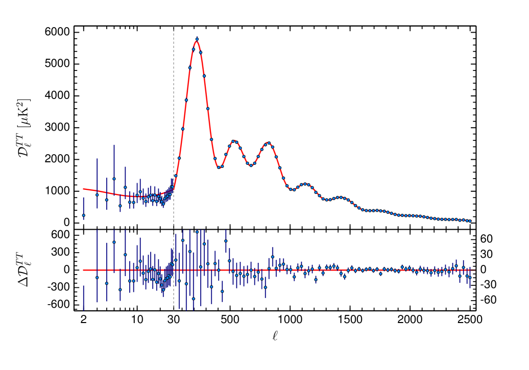
The foreground-subtracted, frequency-averaged, cross-half-mission spectrum is plotted in Fig. 1, together with the Commander power spectrum at multipoles . The high multipole spectrum plotted in this figure is an approximate maximum likelihood solution based on equations (A24) and (A25) of PPL13, with the foregrounds and nuisance parameters for each spectrum fixed to the best-fit values of the base solution. Note that a different way of solving for the Planck CMB spectrum, by marginalizing over foreground and nuisance parameters, is presented in Sect. 4. The best-fit base model is plotted in the upper panel, while residuals with respect to this model are plotted in the lower panel. In this plot, there are only four bandpowers at that differ from the best-fit model by more than . These are: (); (); (); and (). The of the coadded spectrum plotted in Fig. 1 relative to the best-fit base model is for degrees of freedom (), which is a fluctuation (PTE). These numbers confirm the extremely good fit of the base cosmology to the Planck data at high multipoles. The consistency of the Planck polarization spectra with base is discussed in Sect. 3.3.
PCP13 noted some mild internal tensions within the Planck data, for example, the preference of the phenomenological lensing parameter (see Sect. 5.1) towards values greater than unity and a preference for a negative running of the scalar spectral index (see Sect. 6.2.2). These tensions were partly caused by the poor fit of base model to the temperature spectrum at multipoles below about 50. As noted by the WMAP team (Hinshaw et al. 2003), the temperature spectrum has a low quadrupole amplitude and a glitch in the multipole range . These features can be seen in the Planck 2015 spectrum of Fig. 1. They have a similar (though slightly reduced) effect on cosmological parameters to those described in PCP13.
3.2 545-GHz-cleaned spectra
As discussed in PCP13, unresolved extragalactic foregrounds (principally Poisson point sources and the clustered component of the CIB) contribute to the Planck spectra at high multipoles. The approach to modelling these foreground contributions in PCP13 is similar to that used by the ACT and SPT teams (Reichardt et al. 2012; Dunkley et al. 2013) in that the foregrounds are modelled by a set of physically motivated power spectrum template shapes with an associated set of adjustable nuisance parameters. This approach has been adopted as the baseline for the Planck 2015 analysis. The foreground model has been adjusted for this new analysis, in relatively minor ways, as summarized in Sect. 2.3 and described in further detail in Planck Collaboration XII (2016). Galactic dust emission also contributes to the temperature and polarization power spectra and must be subtracted from the spectra used to form the Planck likelihood. Unlike the extragalactic foregrounds, Galactic dust emission is anisotropic and so its impact can be reduced by appropriate masking of the sky. In PCP13, we intentionally adopted conservative masks, tuned for each of the frequencies used to form the likelihood, to keep dust emission at low levels. The results in PCP13 were therefore insensitive to the modelling of residual dust contamination.
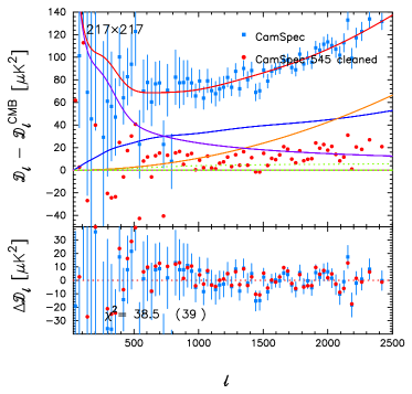
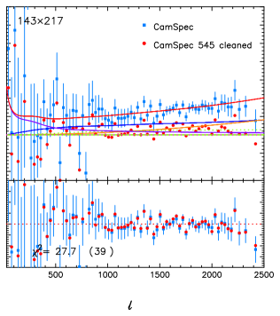
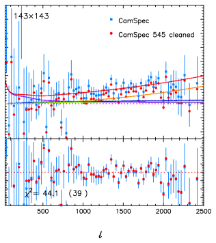
In the 2015 analysis, we have extended the sky coverage at each of 100, 143, and 217 GHz, and so in addition to testing the accuracy of the extragalactic foreground model, it is important to test the accuracy of the Galactic dust model. As described in PPL13 and Planck Collaboration XII (2016) the Galactic dust templates used in the CamSpec and Plik likelihoods are derived by fitting the 545-GHz mask-differenced power spectra. Mask differencing isolates the anisotropic contribution of Galactic dust from the isotropic extragalactic components. For the extended sky coverage used in the 2015 likelihoods, the Galactic dust contributions are a significant fraction of the extragalactic foreground contribution in the temperature spectrum at high multipoles, as illustrated in Fig. 2. Galactic dust dominates over all other foregrounds at multipoles at HFI frequencies.
A simple and direct test of the parametric foreground modelling used in the CamSpec and Plik likelihoods is to compare results with a completely different approach in which the low-frequency maps are “cleaned” using higher frequency maps as foreground templates (see, e.g., Lueker et al. 2010). In a similar approach to Spergel et al. (2015), we can form cleaned maps at lower frequencies by subtracting a 545-GHz map as a template,
| (6) |
where is the frequency of the template map and is the cleaning coefficient. Since the maps have different beams, the subtraction is actually done in the power spectrum domain:
| (7) | |||||
where etc. are the mask-deconvolved beam-corrected power spectra. The coefficients are determined by minimizing
| (8) |
where is the covariance matrix of the estimates . We choose and and compute the spectra in Eq. (7) by cross-correlating half-mission maps on the 60 % mask used to compute the spectrum. The resulting cleaning coefficients are and ; note that all of the input maps are in units of thermodynamic temperature. The cleaning coefficients are therefore optimized to remove Galactic dust at low multipoles, though by using 545 GHz as a dust template we find that the cleaning coefficients are almost constant over the multipole range 50–2500. We note, however, that this is not true if the 353- and 857-GHz maps are used as dust templates, as discussed in Efstathiou et al. (in preparation).
The 545-GHz-cleaned spectra are shown by the red points in Fig. 2 and can be compared directly to the “uncleaned” spectra used in the CamSpec likelihood (upper panels). As can be seen, Galactic dust emission is removed to high accuracy and the residual foreground contribution at high multipoles is strongly suppressed in the and spectra. Nevertheless, there remains small foreground contributions at high multipoles, which we model heuristically as power laws,
| (9) |
with free amplitudes and spectral indices . We construct another CamSpec cross-half-mission likelihood using exactly the same sky masks as the 2015F(CHM) likelihood, but using 545-GHz-cleaned , , and spectra. We then use the simple model of Eq. (9) in the likelihood to remove residual unresolved foregrounds at high multipoles for each frequency combination. We do not clean the spectrum and so for this spectrum we use the standard parametric foreground model in the likelihood. The lower panels in Fig. 2 show the residuals with respect to the best-fit base model and foreground solution for the uncleaned CamSpec spectra (blue points) and for the 545-GHz-cleaned spectra (red points). These residuals are almost identical, despite the very different approaches to Galactic dust removal and foreground modelling. The cosmological parameters from these two likelihoods are also in very good agreement, typically to better than , with the exception of , which is lower in the cleaned likelihood by . It is not surprising, given the heuristic nature of the model (Eq. 9), that shows the largest shift. We can also remove the spectrum from the likelihood entirely, with very little impact on cosmological parameters.
Further tests of map-based cleaning are presented in Planck Collaboration XI (2016), which additionally describes another independently written power-spectrum analysis pipeline (MSPEC) tuned to map-cleaned cross-spectrum analysis and using a more complex model for fitting residual foregrounds than the heuristic model of Eq. (9). Planck Collaboration XI (2016) also describes power spectrum analysis and cosmological parameters derived from component-separated Planck maps. However, the simple demonstration presented in this section shows that the details of modelling residual dust contamination and other foregrounds are under control in the 2015 Planck likelihood. A further strong argument that our results are insensitive to foreground modelling is presented in the next section, which compares the cosmological parameters derived from the , , and likelihoods. Unresolved foregrounds at high multipoles are completely negligible in the polarization spectra and so the consistency of the parameters, particularly from the spectrum (which has higher signal-to-noise than the spectrum) provides an additional cross-check of the results.
Finally, one can ask why we have not chosen to use a 545-GHz-cleaned likelihood as the baseline for the 2015 Planck parameter analysis. Firstly, it would not make any difference to the results of this paper had we chosen to do so. Secondly, we feel that the parametric foreground model used in the baseline likelihood has a sounder physical basis. This allows us to link the amplitudes of the unresolved foregrounds across the various Planck frequencies with the results from other ways of studying foregrounds, including the higher resolution CMB experiments described in Sect. 4.
3.3 The 2015 Planck temperature and polarization spectra and likelihood
|
The coadded 2015 Planck temperature spectrum was introduced in Fig. 1. In this section, we present additional details and consistency checks of the temperature likelihood and describe the full mission Planck and spectra and likelihood; preliminary Planck and spectra were presented in PCP13. We then discuss the consistency of the cosmological parameters for base measured separately from the , , and spectra. For the most part, the discussion given in this section is specific to the Plik likelihood, which is used as the baseline in this paper. A more complete discussion of the Plik and other likelihoods developed by the Planck team is given in Planck Collaboration XI (2016).
3.3.1 Temperature spectra and likelihood
(1) Temperature masks.
As in the 2013 analysis, the high-multipole likelihood uses the , , , and spectra. However, in contrast to the 2013 analysis, which used conservative sky masks to reduce the effects of Galactic dust emission, we make more aggressive use of sky in the 2015 analysis. The 2015 analysis retains 80 %, 70 %, and 60 % of sky at 100 GHz, 143 GHz, and 217 GHz, respectively, before apodization. We also apply apodized point source masks to remove compact sources with a signal-to-noise threshold at each frequency (see Planck Collaboration XXVI 2016 for a description of the Planck Catalogue of Compact Sources). Apodized masks are also applied to remove extended objects, and regions of high CO emission were masked at 100 GHz and 217 GHz (see Planck Collaboration X 2016). As an estimate of the effective sky area, we compute the following sum over pixels:
| (10) |
where is the weight of the apodized mask and is the area of pixel . All input maps are at HEALpix (Górski et al. 2005) resolution . Eq. (10) gives at 100 GHz, 57.4 % at 143 GHz, and 47.1 % at 217 GHz.
(2) Galactic dust templates.
With the increased sky coverage used in the 2015 analysis, we take a slightly different approach to subtracting Galactic dust emission to that described in PPL13 and PCP13. The shape of the Galactic dust template is determined from mask-differenced power spectra estimated from the 545-GHz maps. The mask differencing removes the isotropic contribution from the CIB and point sources. The resulting dust template has a similar shape to the template used in the 2013 analysis, with power-law behaviour at high multipoles, but with a “bump” at (as shown in Fig. 2). The absolute amplitude of the dust templates at 100, 143, and 217 GHz is determined by cross-correlating the temperature maps at these frequencies with the 545-GHz maps (with minor corrections for the CIB and point source contributions). This allows us to generate priors on the dust template amplitudes, which are treated as additional nuisance parameters when running MCMC chains (unlike the 2013 analysis, in which we fixed the amplitudes of the dust templates). The actual priors used in the Plik likelihood are Gaussians on with the following means and dispersions: K2 for the spectrum; K2 for ; K2 for ; and K2 for . The MCMC solutions show small movements of the best-fit dust template amplitudes, but always within statistically acceptable ranges given the priors.
(3) Likelihood approximation and covariance matrices.
The approximation to the likelihood function follows the methodology described in PPL13 and is based on a Gaussian likelihood assuming a fiducial theoretical power spectrum (a fit to Plik TT with prior ). We have also included a number of small refinements to the covariance matrices. Foregrounds, including Galactic dust, are added to the fiducial theoretical power spectrum, so that the additional small variance associated with foregrounds is included, along with cosmic variance of the CMB, under the assumption that the foregrounds are Gaussian random fields. The 2013 analysis did not include corrections to the covariance matrices arising from leakage of low-multipole power to high multipoles via the point source holes; these can introduce errors in the covariance matrices of a few percent at , corresponding approximately to the first peak of the CMB spectrum. In the 2015 analysis we apply corrections to the fiducial theoretical power spectrum, based on Monte Carlo simulations, to correct for this effect. We also apply Monte Carlo based corrections to the analytic covariance matrices at multipoles , where the analytic approximations begin to become inaccurate even for large effective sky areas (see Efstathiou 2004). Finally, we add the uncertainties on the beam shapes to the covariance matrix following the methodology described in PPL13. The Planck beams are much more accurately characterized in the 2015 analysis, and so the beam corrections to the covariance matrices are extremely small. The refinements to the covariance matrices described in this paragraph are all relatively minor and have little impact on cosmological parameters.
(4) Binning.
The baseline Plik likelihood uses binned temperature and polarization spectra. This is done because all frequency combinations of the and spectra are used in the Plik likelihood, leading to a large data vector of length if the spectra are retained multipole-by-multipole. The baseline Plik likelihood reduces the size of the data vector by binning these spectra. The spectra are binned into bins of width for , for , for and for , with a weighting of proportional to over the bin widths. The bins span an odd number of multipoles, since for approximately azimuthal masks we expect a nearly symmetrical correlation function around the central multipole. The binning does not affect the determination of cosmological parameters in -type models (which have smooth power spectra), but significantly reduces the size of the joint TT,TE,EE covariance matrix, speeding up the computation of the likelihood. However, for some specific purposes, e.g., searching for oscillatory features in the spectrum, or testing statistics, we produce blocks of the likelihood multipole-by-multipole.
(5) Goodness of fit.
The first five rows of Table 2 list statistics for the spectra (multipole-by-multipole) relative to the Planck best-fit base model and foreground parameters (fitted to Planck TT+lowP). The first four entries list the statistics separately for each of the four spectra that form the likelihood and the fifth line (labelled “Combined”) gives the value for the maximum likelihood spectrum plotted in Fig. 1. Each of the individual spectra provides an acceptable fit to the base model, as does the frequency-averaged spectrum plotted in Fig. 1. This demonstrates the excellent consistency of the base model across frequencies. More detailed consistency checks of the Planck spectra are presented in Planck Collaboration XI (2016); however, as indicated by Table 2, we find no evidence for any inconsistencies between the foreground-corrected temperature power spectra computed for different frequency combinations. The temperature spectra are largely signal dominated over the multipole ranges listed in Table 2 and so the values are insensitive to small errors in the Planck noise model used in the covariance matrices. As discussed in the next subsection, this is not true for the and spectra, which are noise dominated over much of the multipole range.
3.3.2 Polarization spectra and likelihood
In addition to the spectra, the 2015 Planck likelihood includes the and spectra. As discussed in Sect. 3.1, the Planck 2015 low-multipole polarization analysis is based on the LFI 70-GHz data. Here we discuss the and spectra that are used in the high-multipole likelihood, which are computed from the HFI data at , and GHz. As summarized in Planck Collaboration XI (2016), there is no evidence for any unresolved foreground components at high multipoles in the polarization spectra. We therefore include all frequency combinations in computing the and spectra to maximize the signal-to-noise.111111In temperature, the and spectra are not included in the likelihood because the temperature spectra are largely signal dominated. These spectra therefore add little new information on the CMB, but would require additional nuisance parameters to correct for unresolved foregrounds at high multipoles.
(1) Masks and dust corrections.
At low multipoles () polarized Galactic dust emission is significant at all frequencies and is subtracted in a similar way to the dust subtraction in temperature, i.e., by including additional nuisance parameters quantifying the amplitudes of a power-law dust template with a slope constrained to for both and (Planck Collaboration Int. XXX 2016). Polarized synchrotron emission (which has been shown to be negligible at 100 GHz and higher frequencies for Planck noise levels, Fuskeland et al. 2014) is ignored. Gaussian priors on the polarization dust amplitudes are determined by cross-correlating the lower frequency maps with the 353-GHz polarization maps (the highest frequency polarized channel of the HFI) in a similar way to the determination of temperature dust priors. We use the temperature-based apodized masks in and at each frequency, retaining 70 %, 50 %, and 41 % of the sky at 100, 143, and 217 GHz, respectively, after apodization (slightly smaller than the temperature masks at 143 and 217 GHz). However, we do not apply point source or CO masks to the and maps. The construction of the full TT,TE,EE likelihood is then a straightforward extension of the likelihood using the analytic covariance matrices given by Efstathiou (2006) and Hamimeche & Lewis (2008).
(2) Polarization spectra and residual systematics.
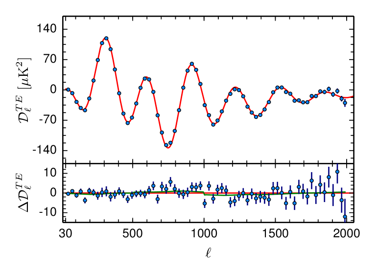
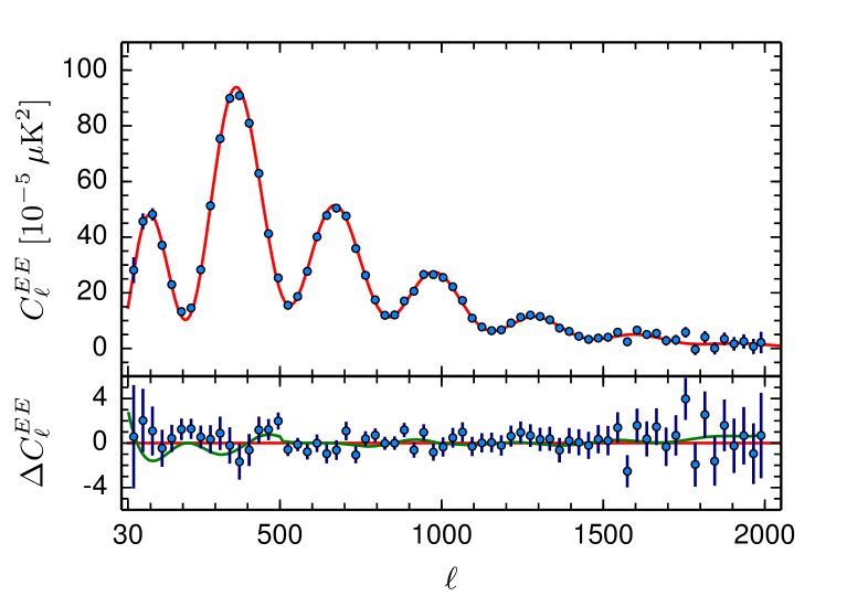
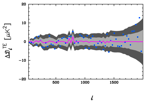
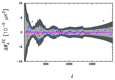
Maximum likelihood frequency coadded and spectra are shown in Fig. 3. The theoretical curves plotted in these figures are the and spectra computed from the best-fit base model fitted to the temperature spectra (Planck TT+lowP), as plotted in Fig. 1. The lower panels in each figure show the residuals with respect to this model. The theoretical model provides a very good fit to the and spectra. Table 2 lists statistics for the and spectra for each frequency combination (with the and spectra for each frequency combination coadded to form a single spectrum). Note that since the and spectra are noisier than the spectra, these values of are sensitive to the procedure used to estimate Planck noise (see Planck Collaboration XI 2016 for further details).
Some of these values are unusually high, for example the and spectra and the spectrum all have low PTEs. The Planck and spectra for different frequency combinations are not as internally consistent as the Planck spectra. Inter-comparison of the and spectra at different frequencies is much more straightforward than for the temperature spectra because unresolved foregrounds are unimportant in polarization. The high values listed in Table 2 therefore provide clear evidence of residual instrumental systematics in the and spectra.
With our present understanding of the Planck polarization data, we believe that the dominant source of systematic error in the polarization spectra is caused by beam mismatch that generates leakage from temperature to polarization (recalling that the HFI polarization maps are generated by differencing signals between quadruplets of polarization sensitive bolometers). In principle, with accurate knowledge of the beams this leakage could be described by effective polarized beam window functions. For the 2015 papers, we use the beams rather than polarized beams, and characterize temperature-to-polarization leakage using a simplified model. The impact of beam mismatch on the polarization spectra in this model is
| (0a) | |||||
| (0b) |
where is a polynomial in multipole. As a consequence of the Planck scanning strategy, pixels are visited approximately every six months, with a rotation of the focal plane by , leading to a weak coupling to beam modes with odd values of . The dominant contributions are expected to come from modes with and , describing the beam ellipticity. We therefore fit the spectra using a fourth-order polynomial,
| (1) |
treating the coefficients , , and as nuisance parameters in the MCMC analysis. We have ignored the odd coefficients of the polynomial, which should be suppressed by our scanning strategy. We do however include a constant term in the polynomial to account for small deviations of the polarization efficiency from unity.
The fit is performed separately on the and spectra. A different polynomial is used for each cross-frequency spectrum. The coadded corrections are shown in the lower panels of Fig. 3. Empirically, we find that temperature-to-polarization leakage systematics tend to cancel in the coadded spectra. Although the best-fit leakage corrections to the coadded spectra are small, the corrections for individual frequency cross-spectra can be up to 3 times larger than those shown in Fig. 3. The model of Eqs. (0a) and (0b) is clearly crude, but gives us some idea of the impact of temperature-to-polarization leakage in the coadded spectra. With our present empirical understanding of leakage, we find a correlation between the polarization spectra that have the highest expected temperature-to-polarization leakage and those that display high in Table 2. However, the characterization of this leakage is not yet accurate enough to reduce the values for each frequency combination to acceptable levels.
As discussed in PCP13, each Planck data release and accompanying set of papers should be viewed as a snapshot of the state of the Planck analysis at the time of the release. For the 2015 release, we have a high level of confidence in the temperature power spectra. However, we have definite evidence for low-level systematics associated with temperature-to-polarization leakage in the polarization spectra. The tests described above suggest that these are at low levels of a few in . However, temperature-to-polarization leakage can introduce correlated features in the spectra, as shown by the leakage model plotted in Fig. 3. Until we have a more accurate characterization of these systematics, we urge caution in the interpretation of features in the and spectra. For some of the 2015 papers, we use the and spectra, without leakage corrections. For most of the models considered in this paper, the spectra alone provide tight constraints and so we take a conservative approach and usually quote the results. However, as we will see, we find a high level of consistency between the Planck and full Planck likelihoods. Some models considered in Sect. 6 are, however, sensitive to the polarization blocks of the likelihood. Examples include constraints on isocurvature modes, dark matter annihilation, and non-standard recombination histories. Planck 2015 constraints on these models should be viewed as preliminary, pending a more complete analysis of polarization systematics, which will be presented in the next series of Planck papers accompanying a third data release.
| Parameter [1] Planck TT+lowP [2] Planck TE+lowP [3] Planck EE+lowP [4] Planck TT,TE,EE+lowP . . . . . . . . . . |
(3) and conditionals.
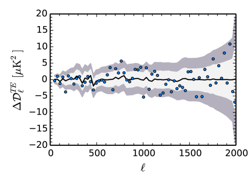
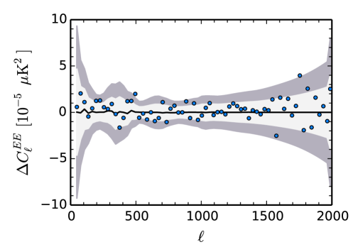
Given the best-fit base cosmology and foreground parameters determined from the temperature spectra, one can test whether the and spectra are consistent with the spectra by computing conditional probabilities. Writing the data vector as
| (2) |
where the quantities , , and are the maximum likelihood freqency co-added foreground-corrected spectra. The covariance matrix of this vector can be partitioned as
| (3) |
The expected value of the polarization vector, given the observed temperature vector is
| (4) |
with covariance
| (5) |
In Eq. (4), and are the theoretical temperature and polarization spectra deduced from minimizing the Planck TT+lowP likelihood. Equations (4) and (5) give the expectation values and distributions of the polarization spectra conditional on the observed temperature spectra. These are shown in Fig. 4. Almost all of the data points sit within the bands and in the case of the spectra, the data points track the fluctuations expected from the spectra at multipoles . Figure 4 therefore provides an important additional check of the consistency of the and spectra with the base cosmology.
(4) Likelihood implementation.
Section 3.1 showed good consistency between the independently written CamSpec and Plik codes in temperature. The methodology used for the temperature likelihoods are very similar, but the treatment of the polarization spectra in the two codes differs substantially. CamSpec uses low-resolution CMB-subtracted 353-GHz polarization maps thresholded by to define diffuse Galactic polarization masks. The same apodized polarization mask, with an effective sky fraction (as defined by Eq. (10)), is used for 100-, 143-, and 217-GHz and maps. Since there are no unresolved extragalactic foregrounds detected in the and spectra, all of the different frequency combinations of and spectra are compressed into single and spectra (weighted by the inverse of the diagonals of the appropriate covariance matrices), after foreground cleaning using the 353-GHz maps121212To reduce the impact of noise at 353 GHz, the map-based cleaning of the and spectra is applied at . At higher multipoles, the polarized dust corrections are small and are subtracted as power laws fitted to the Galactic dust spectra at lower multipoles. (generalizing the map cleaning technique described in Sect. 3.2 to polarization). This allows the construction of a full likelihood with no binning of the spectra and with no additional nuisance parameters in polarization. As noted in Sect. 3.1 the consistency of results from the polarization blocks of the CamSpec and Plik likelihoods is not as good as in temperature. Cosmological parameters from fits to the and CamSpec and Plik likelihoods can differ by up to about , although no major science conclusions would change had we chosen to use the CamSpec likelihood as the baseline in this paper. We will, however, sometimes quote results from CamSpec in addition to those from Plik to give the reader an indication of the uncertainties in polarization associated with different likelihood implementations. Figure 5 shows the CamSpec and residuals and error ranges conditional on the best-fit base and foreground model fitted to the CamSpec temperature+lowP likelihood. The residuals in both and are similar to those from Plik. The main difference can be seen at low multipoles in the spectrum, where CamSpec shows a higher dispersion, consistent with the error model, though there are several high points at corresponding to the minimum in the spectrum, which may be caused by small errors in the subtraction of polarized Galactic emission using 353 GHz as a foreground template (and there are also differences in the covariance matrices at high multipoles caused by differences in the methods used in CamSpec and Plik to estimate noise). Generally, cosmological parameters determined from the CamSpec likelihood have smaller formal errors than those from Plik because there are no nuisance parameters describing polarized Galactic foregrounds in CamSpec.
3.3.3 Consistency of cosmological parameters from the , , and spectra
The consistency between parameters of the base model determined from the Plik temperature and polarization spectra are summarized in Table 3 and in Fig. 6. As pointed out by Zaldarriaga et al. (1997) and Galli et al. (2014), precision measurements of the CMB polarization spectra have the potential to constrain cosmological parameters to higher accuracy than measurements of the spectra because the acoustic peaks are narrower in polarization and unresolved foreground contributions at high multipoles are much lower in polarization than in temperature. The entries in Table 3 show that cosmological parameters that do not depend strongly on are consistent between the and spectra, to within typically or better. Furthermore, the cosmological parameters derived from the spectra have comparable errors to the parameters. None of the conclusions in this paper would change in any significant way were we to use the parameters in place of the parameters. The consistency of the cosmological parameters for base between temperature and polarization therefore gives added confidence that Planck parameters are insensitive to the specific details of the foreground model that we have used to correct the spectra. The parameters are also typically within about of the parameters, though because the spectra from Planck are noisier than the spectra, the errors on the parameters are significantly larger than those from . However, both the and likelihoods give lower values of , and , by over compared to the solutions. Noticee that the and EE entries in Table 3 do not use any information from the temperature in the low-multipole likelihood. The tendency for higher values of , , and in the Planck TT+lowP solution is driven, in part, by the temperature power spectrum at low multipoles.
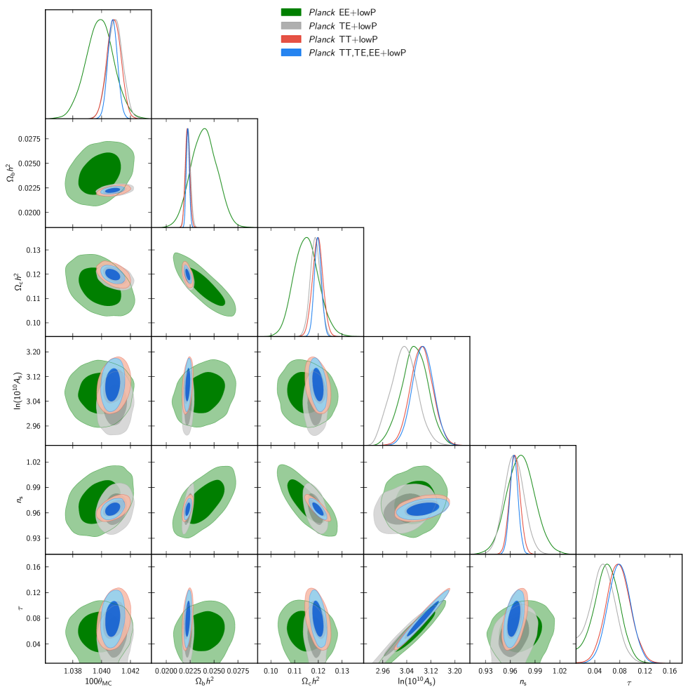
Columns [4] and [5] of Table 3 compare the parameters of the Planck likelihood with the full Planck likelihood. These are in agreement, shifting by less than . Although we have emphasized the presence of systematic effects in the Planck polarization spectra, which are not accounted for in the errors quoted in column [4] of Table 3, the consistency of the Planck and Planck parameters provides strong evidence that residual systematics in the polarization spectra have little impact on the scientific conclusions in this paper. The consistency of the base parameters from temperature and polarization is illustrated graphically in Fig. 6. As a rough rule-of-thumb, for base , or extensions to with spatially flat geometry, using the full Planck likelihood produces improvements in cosmological parameters of about the same size as adding BAO to the Planck TT+lowP likelihood.
3.4 Constraints on the reionization optical depth parameter
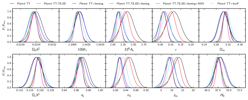
The reionization optical depth parameter provides an important constraint on models of early galaxy evolution and star formation. The evolution of the inter-galactic Ly opacity measured in the spectra of quasars can be used to set limits on the epoch of reionization (Gunn & Peterson 1965). The most recent measurements suggest that the reionization of the inter-galactic medium was largely complete by a redshift (Fan et al. 2006). The steep decline in the space density of Ly-emitting galaxies over the redshift range also implies a low redshift of reionization (Choudhury et al. 2015). As a reference, for the Planck parameters listed in Table 3, instantaneous reionization at redshift results in an optical depth of .
The optical depth can also be constrained from observations of the CMB. The WMAP9 results of Bennett et al. (2013) give , corresponding to an instantaneous redshift of reionization . The WMAP constraint comes mainly from the spectrum in the multipole range –6. It has been argued (e.g., Robertson et al. 2013, and references therein) that the high optical depth reported by WMAP cannot be produced by galaxies seen in deep redshift surveys, even assuming high escape fractions for ionizing photons, implying additional sources of photoionizing radiation from still fainter objects. Evidently, it would be useful to have an independent CMB measurement of .
The measurement from CMB polarization is difficult because it is a small signal, confined to low multipoles, requiring accurate control of instrumental systematics and polarized foreground emission. As discussed by Komatsu et al. (2009), uncertainties in modelling polarized foreground emission are comparable to the statistical error in the WMAP measurement. In particular, at the time of the WMAP9 analysis there was very little information available on polarized dust emission. This situation has been partially rectified by the 353-GHz polarization maps from Planck (Planck Collaboration Int. XXII 2015; Planck Collaboration Int. XXX 2016). In PPL13, we used preliminary 353-GHz Planck polarization maps to clean the WMAP Ka, Q, and V maps for polarized dust emission, using WMAP K-band as a template for polarized synchrotron emission. This lowered by about 1 to , compared to using the WMAP dust model.131313Neither of these error estimates reflect the true uncertainty in foreground removal. However, given the preliminary nature of the Planck polarization analysis we decided for the Planck 2013 papers to use the WMAP polarization likelihood, as produced by the WMAP team.
In the 2015 papers, we use Planck polarization maps based on low-resolution LFI 70-GHz maps, excluding Surveys 2 and 4. These maps are foreground-cleaned using the LFI 30-GHz and HFI 353-GHz maps as polarized synchrotron and dust templates, respectively. These cleaned maps form the polarization part (“lowP’ ) of the low-multipole Planck pixel-based likelihood, as described in Planck Collaboration XI (2016). The temperature part of this likelihood is provided by the Commander component-separation algorithm. The Planck low-multipole likelihood retains 46 % of the sky in polarization and is completely independent of the WMAP polarization likelihood. In combination with the Planck high multipole likelihood, the Planck low-multipole likelihood gives . This constraint is somewhat higher than the constraint derived from the Planck low-multipole likelihood alone (see Planck Collaboration XI 2016 and also Sect. 5.1.2).
Following the 2013 analysis, we have used the 2015 HFI 353-GHz polarization maps as a dust template, together with the WMAP K-band data as a template for polarized synchrotron emission, to clean the low-resolution WMAP Ka, Q, and V maps (see Planck Collaboration XI 2016 for further details). For the purpose of cosmological parameter estimation, this data set is masked using the WMAP P06 mask, which retains 73 % of the sky. The noise-weighted combination of the Planck 353-cleaned WMAP polarization maps yields when combined with the Planck information in the range , consistent with the value of obtained from the LFI 70-GHz polarization maps. In fact, null tests described in Planck Collaboration XI (2016) demonstrate that the LFI and WMAP polarization data are statistically consistent. The HFI polarization maps have higher signal-to-noise than the LFI and could, in principle, provide a third cross-check. However, at the time of writing, we are not yet confident that systematics in the HFI maps at low multipoles () are at negligible levels. A discussion of HFI polarization at low multipoles will therefore be deferred to future papers.141414See Planck Collaboration Int. XLVI (2016), which has been submitted since this paper was written.
Given the difficulty of making accurate CMB polarization measurements at low multipoles, it is useful to investigate other ways of constraining . Measurements of the temperature power spectrum provide a highly accurate measurement of the amplitude . However, as shown in PCP13 CMB lensing breaks the degeneracy between and . The observed Planck spectrum is, of course, lensed, so the degeneracy between and is partially broken when we fit models to the Planck likelihood. However, the degeneracy breaking is much stronger if we combine the Planck TT likelihood with the Planck lensing likelihood constructed from measurements of the power spectrum of the lensing potential . The 2015 Planck TT and lensing likelihoods are statistically more powerful than their counterparts and the corresponding determination of is more precise. The 2015 Planck lensing likelihood (labelled “lensing”) is summarized in Sec. 5.1 and discussed in more detail in Planck Collaboration XV (2016). The constraints on and 151515We use the same specific definition of as in the papers, where reionization is assumed to be relatively sharp, with a mid-point parameterized by a redshift and width . Unless otherwise stated we impose a flat prior on the optical depth with . for various data combinations excluding low-multipole polarization data from Planck are summarized in Fig. 7 and compared with the baseline Planck TT+lowP parameters. This figure also shows the shifts of other parameters of the base cosmology, illustrating their sensitivity to changes in .
The Planck constraints on and in the base model for various data combinations are:
| (0a) | |||||
| (0b) | |||||
The constraint from Planck TT+lensing+BAO on is completely independent of low-multipole CMB polarization data and agrees well with the result from Planck polarization (and has comparable precision). These results all indicate a lower redshift of reionization than the value derived in PCP13, based on the WMAP9 polarization likelihood. The low values of from Planck are also consistent with the lower value of derived from the WMAP Planck 353-GHz-cleaned polarization likelihood, suggesting strongly that the WMAP9 value is biased slightly high by residual polarized dust emission.
The Planck results of Eqs. (0a)–(3.4) provide evidence for a lower optical depth and redshift of reionization than inferred from WMAP (Bennett et al. 2013), partially alleviating the difficulties in reionizing the intergalactic medium using starlight from high-redshift galaxies. A key goal of the Planck analysis over the next year is to assess whether these results are consistent with the HFI polarization data at low multipoles.
Given the consistency between the LFI and WMAP polarization maps when both are cleaned with the HFI 353-GHz polarization maps, we have also constructed a combined WMAP+Planck low-multipole polarization likelihood (denoted “lowP+WP”). This likelihood uses 73 % of the sky and is constructed from a noise-weighted combination of LFI 70-GHz and WMAP Ka, Q, and V maps, as summarized in Sect. 3.1 and discussed in more detail in Planck Collaboration XI (2016). In combination with the Planck high-multipole likelihood, the combined lowP+WP likelihood gives , consistent with the individual LFI and WMAP likelihoods to within about .
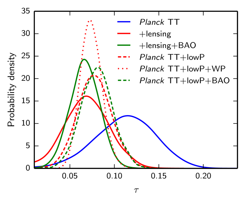
The various Planck and Planck+WMAP constraints on are summarized in Fig. 8. The tightest of these constraints comes from the combined lowP+WP likelihood. It is therefore reasonable to ask why we have chosen to use the lowP likelihood as the baseline in this paper, which gives a higher statistical error on . The principal reason is to produce a Planck analysis, utilizing the LFI polarization data, that is independent of WMAP. All of the constraints shown in Fig. 8 are compatible with each other, and insofar as other cosmological parameters are sensitive to small changes in , it would make very little difference to the results in this paper had we chosen to use WMAP or Planck+WMAP polarization data at low multipoles.
4 Comparison of the Planck power spectrum with high-resolution experiments
In PCP13 we combined Planck with the small-scale measurements of the ground-based, high-resolution Atacama Cosmology Telescope (ACT) and South Pole Telescope (SPT). The primary role of using ACT and SPT was to set limits on foreground components that were poorly constrained by Planck alone and to provide more accurate constraints on the damping tail of the temperature power spectrum. In this paper, with the higher signal-to-noise levels of the full mission Planck data, we have taken a different approach, using the ACT and SPT data to impose a prior on the thermal and kinetic SZ power spectrum parameters in the Planck foreground model as described in Sect. 2.3. In this section, we check the consistency of the temperature power spectra measured by Planck, ACT, and SPT, and test the effects of including the ACT and SPT data on the recovered CMB power spectrum.
We use the latest ACT temperature power spectra presented in Das et al. (2014), with a revised binning described in Calabrese et al. (2013) and final beam estimates in Hasselfield et al. (2013). As in PCP13 we use ACT data in the range at 148 GHz, and for the and 218-GHz spectra. We use SPT measurements in the range from the complete SPT-SZ survey at 95, 150, and 220 GHz presented in George et al. (2015).
Each of these experiments uses a foreground model to describe the multi-frequency power spectra. Here we implement a common foreground model to combine Planck with the high-multipole data, following a similar approach to PCP13 but with some refinements. Following the 2013 analysis, we solve for common nuisance parameters describing the tSZ, kSZ, and tSZCIB components, extending the templates used for Planck to to cover the full ACT and SPT multipole range. As in PCP13, we use five point-source amplitudes to fit for the total dusty and radio Poisson power, namely , , , , and . We rescale these amplitudes to cross-frequency spectra using point-source correlation coefficients, improving on the 2013 treatment by using different parameters for the ACT and SPT correlations, and (a single parameter was used in 2013). We vary and as in 2013, and include dust amplitudes for ACT, with Gaussian priors as in PCP13.
As described in Sect. 2.3 we use a theoretically motivated clustered CIB model fitted to Planck+IRAS estimates of the CIB. The model at all frequencies in the range 95–220 GHz is specified by a single amplitude . The CIB power is well constrained by Planck data at . At multipoles , the 1-halo component of the CIB model steepens and becomes degenerate with the Poisson power. This causes an underestimate of the Poisson levels for ACT and SPT, inconsistent with predictions from source counts. We therefore use the Planck CIB template only in the range , and extrapolate to higher multipoles using a power law . While this may not be a completely accurate model for the clustered CIB spectrum at high multipoles (see, e.g., Viero et al. 2013; Planck Collaboration XXX 2014), this extrapolation is consistent with the CIB model used in the analysis of ACT and SPT. We then need to extrapolate the Planck 217-GHz CIB power to the ACT and SPT frequencies. This requires converting the CIB measurement in the HFI 217-GHz channel to the ACT and SPT bandpasses assuming a spectral energy distribution; we use the CIB spectral energy distribution from Béthermin et al. (2012). Combining this model with the ACT and SPT bandpasses, we find that has to be multiplied by 0.12 and 0.89 for ACT 148 and 218 GHz, and by 0.026, 0.14, and 0.91 for SPT 95, 150, and 220 GHz, respectively. With this model in place, the best-fit Planck, ACT, and SPT Poisson levels agree with those predicted from source counts, as discussed further in Planck Collaboration XI (2016).
The nuisance model includes seven calibration parameters as in PCP13 (four for ACT and three for SPT). The ACT spectra are internally calibrated using the WMAP 9-year maps, with 2 % and 7 % uncertainty at 148 and 218 GHz, while SPT calibrates using the Planck 2013 143-GHz maps, with 1.1 %, 1.2 %, and 2.2 % uncertainty at 95, 150, and 220 GHz. To account for the increased 2015 Planck absolute calibration (2 % higher in power) we increase the mean of the SPT map-based calibrations from 1.00 to 1.01.
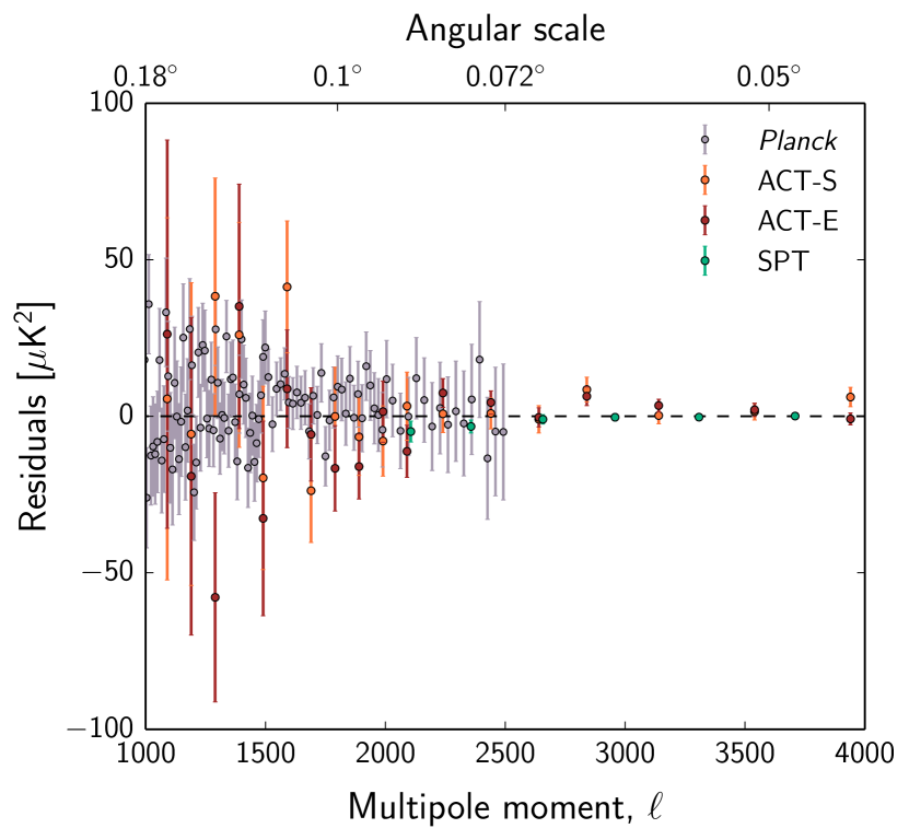
This common foreground and calibration model fits the data well. We first fix the cosmology to that of the best-fit Planck TT+lowP base- model, and estimate the foreground and calibration parameters, finding a best-fitting of 734 for 731 degrees of freedom (reduced , PTE = 0.46). We then simultaneously estimate the Planck, ACT- (S: south, E: equatorial) and SPT CMB bandpowers, , following the Gibbs sampling scheme of Dunkley et al. (2013) and Calabrese et al. (2013), marginalizing over the nuisance parameters.
To simultaneously solve for the Planck, ACT, and SPT CMB spectra, we extend the nuisance model described above, including the four Planck point source amplitudes, the dust parameters and the Planck 100-GHz and 217-GHz calibration parameters (relative to 143 GHz) with the same priors as used in the Planck multi-frequency likelihood analysis. For ACT and SPT, the calibration factors are defined for each frequency (rather than relative to a central frequency). Following Calabrese et al. (2013), we separate out the 148-GHz calibration for the ACT-(S,E) spectra and the 150-GHz calibration for SPT, estimating the CMB bandpowers as .161616This means that the other calibration factors (e.g., ACT 218 GHz) are re-defined to be relative to 148 GHz (or 150 GHz for SPT) data. We impose Gaussian priors on : for ACT-(S,E); and for SPT. The estimated CMB spectrum will then have an overall calibration uncertainty for each of the ACT-S, ACT-E, and SPT spectra. We do not require the Planck CMB bandpowers to be the same as those for ACT or SPT, so that we can check for consistency between the three experiments.
In Fig. 9 we show the residual CMB power with respect to the Planck TT+lowP best-fit model for the three experiments. All of the data sets are consistent over the multipole range plotted in this figure. For ACT-S, we find (18 data points, ); For ACT-E we find (18 data points, ); and for SPT (6 data points, ).
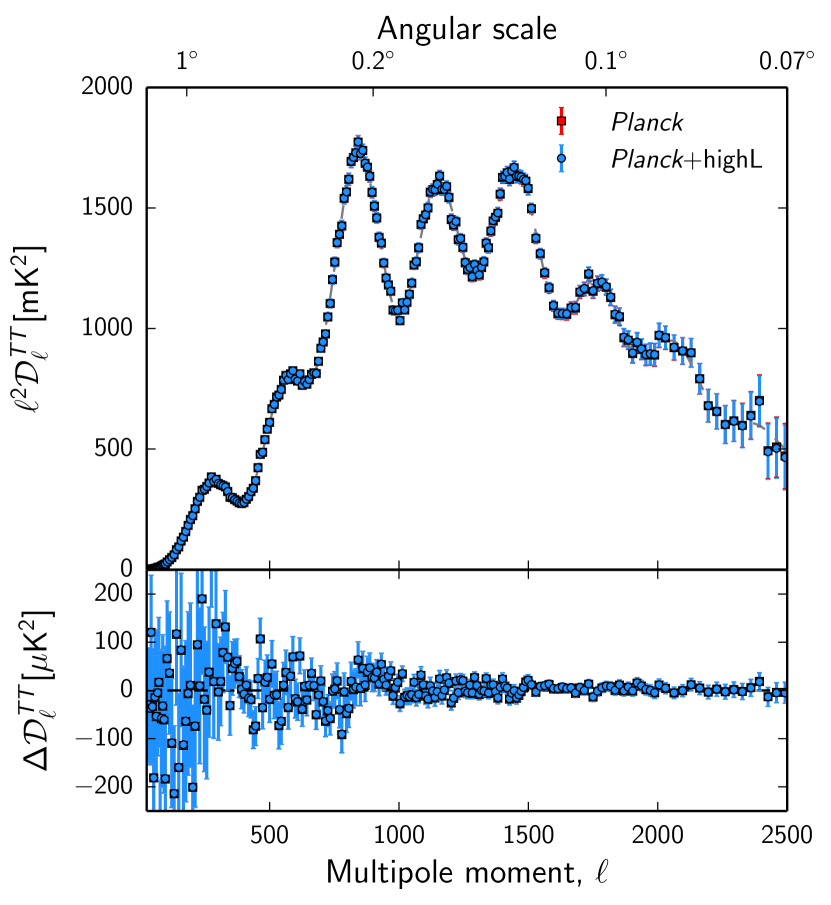
Figure 10 shows the effect of including ACT and SPT data on the recovered Planck CMB spectrum. We find that including the ACT and SPT data does not reduce the Planck errors significantly. This is expected because the dominant small-scale foreground contributions for Planck are the Poisson source amplitudes, which are treated independently of the Poisson amplitudes for ACT and SPT. The high-resolution experiments do help tighten the CIB amplitude (which is reasonably well constrained by Planck) and the tSZ and kSZ amplitudes (which are sub-dominant foregrounds for Planck). The kSZ effect in particular is degenerate with the CMB, since both have blackbody components; imposing a prior on the allowed kSZ power (as discussed in Sect. 2.3) breaks this degeneracy. The net effect is that the errors on the recovered Planck CMB spectrum are only marginally reduced with the inclusion of the ACT and SPT data. This motivates our choice to include the information from ACT and SPT into the joint tSZ and kSZ prior applied to Planck.
The Gibbs sampling technique recovers a best-fit CMB spectrum marginalized over foregrounds and other nuisance parameters. The Gibbs samples can then be used to form a fast CMB-only Planck likelihood that depends on only one nuisance parameter, the overall calibration . MCMC chains run using the CMB-only likelihood therefore converge much faster than using the full multi-frequency Plik likelihood. The CMB-only likelihood is also extremely accurate, even for extensions to the base cosmology and is discussed further in Planck Collaboration XI (2016).
5 Comparison of the Planck base model with other astrophysical data sets
5.1 CMB lensing measured by Planck
Gravitational lensing by large-scale structure leaves imprints on the CMB temperature and polarization that can be measured in high angular resolution, low-noise observations, such as those from Planck. The most relevant effects are a smoothing of the acoustic peaks and troughs in the , , and power spectra, the conversion of -mode polarization to -modes, and the generation of significant non-Gaussianity in the form of a non-zero connected 4-point function (see Lewis & Challinor 2006 for a review). The latter is proportional to the power spectrum of the lensing potential , and so one can estimate this power spectrum from the CMB 4-point functions. In the 2013 Planck release, we reported a detection of the lensing effect in the power spectrum (see PCP13) and a measurement of the amplitude of from the 4-point function (Planck Collaboration XVII 2014). The power of such lensing measurements is that they provide sensitivity to parameters that affect the late-time expansion, geometry, and matter clustering (e.g., spatial curvature and neutrino masses) from the CMB alone.
Since the 2013 Planck release, there have been significant developments in the field of CMB lensing. The SPT team have reported a detection of lens-induced -mode polarization based on the 3-point function, where is a proxy for the CMB lensing potential derived from CIB measurements (Hanson et al. 2013). The POLARBEAR collaboration (POLARBEAR Collaboration 2014b) and the ACT collaboration (van Engelen et al. 2015) have performed similar analyses at somewhat lower significance (POLARBEAR Collaboration 2014b). In addition, the first detections of the polarization 4-point function from lensing, at a significance of around , have been reported by the POLARBEAR (Ade et al. 2014) and SPT (Story et al. 2015) collaborations, and the former have also made a direct measurement of the power spectrum due to lensing on small angular scales with a significance around (POLARBEAR Collaboration 2014a). Finally, the power spectrum from lensing has also been detected on degree angular scales, with similar significance, by the BICEP2 collaboration (BICEP2 Collaboration 2014); see also BKP.
5.1.1 The Planck lensing likelihood
Lensing results from the full-mission Planck data are discussed in Planck Collaboration XV (2016).171717In that paper we are careful to highlight the 4-point function origin of the lensing power spectrum reconstruction by using the index ; however, in this paper we use the notation . With approximately twice the amount of temperature data, and the inclusion of polarization, the noise levels on the reconstructed are a factor of about 2 better than in Planck Collaboration XVII (2014). The broad-band amplitude of is now measured to better than accuracy, the most significant measurement of CMB lensing to date. Moreover, lensing -modes are detected at , both through a correlation analysis with the CIB and via the 4-point function. Many of the results in this paper make use of the Planck measurements of . In particular, they provide an alternative route to estimate the optical depth (as already discussed in Sect. 3.4), and to tightly constrain spatial curvature (Sect. 6.2.4).
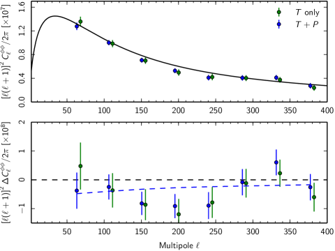
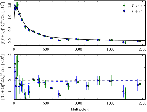
The estimation of from the Planck full-mission data is discussed in detail in Planck Collaboration XV (2016). There are a number of significant changes from the 2013 analysis that are worth noting here.
-
The lensing potential power spectrum is now estimated from lens reconstructions that use both temperature and polarization data in the multipole range . The likelihood used here is based on the power spectrum of a lens reconstruction derived from the minimum-variance combination of five quadratic estimators (, , , , and ). The power spectrum is therefore based on 15 different 4-point functions.
-
The results used here are derived from foreground-cleaned maps of the CMB synthesized from all nine Planck frequency maps with the SMICA algorithm, while the baseline 2013 results used a minimum-variance combination of the 143-GHz and 217-GHz nominal-mission maps. After masking the Galaxy and point-sources, of the sky is retained for the lensing analysis.
-
The lensing power spectrum is estimated in the multipole range . Multipoles have large mean-field corrections due to survey anisotropy and are rather unstable to analysis choices; they are therefore excluded from all lensing results. Here, we use only the range (the same as used in the 2013 analysis), with eight bins each of width . This choice is based on the extensive suite of null tests reported in Planck Collaboration XV (2016). Nearly all tests are passed over the full multipole range , with the exception of a slight excess of curl modes in the reconstruction around . Given that the range contains most of the statistical power in the reconstruction, we have conservatively adopted this range for use in the Planck 2015 cosmology papers.
-
To normalize from the measured 4-point functions requires knowledge of the CMB power spectra. In practice, we normalize with fiducial spectra, but then correct for changes in the true normalization at each point in parameter space within the likelihood. The exact renormalization scheme adopted in the 2013 analysis proved to be too slow for the extension to polarization, so we now use a linearized approximation, based on pre-computed response functions, which is very efficient within an MCMC analysis. Spot-checks have confirmed the accuracy of this approach.
-
The measurement of can be thought of as being derived from an optimal combination of trispectrum configurations. In practice, the expectation value of this combination at any multipole has a local part proportional to , but also a non-local (“ bias”) part that couples to a broad range of multipoles in (Kesden et al. 2003); this non-local part comes from non-primary trispectrum couplings. In the Planck 2013 analysis we corrected for the bias by making a fiducial correction, but this ignores its parameter dependence. We improve on this in the 2015 analysis by correcting for errors in the fiducial bias at each point in parameter space within the lensing likelihood. As with the renormalization above, we linearize this correction for efficiency. As a result, we no longer need to make an approximate correction in the covariance matrix to account for the cosmological uncertainty in .
-
Beam uncertainties are no longer included in the covariance matrix of , since, with the improved knowledge of the beams, the estimated uncertainties are negligible for the lensing analysis. The only inter-bandpower correlations included in the bandpower covariance matrix are from the uncertainty in the correction applied for the point-source 4-point function.
As in the 2013 analysis, we approximate the lensing likelihood as Gaussian in the estimated bandpowers, with a fiducial covariance matrix. Following the arguments in Schmittfull et al. (2013), it is a good approximation to ignore correlations between the 2- and 4-point functions; so, when combining the Planck power spectra with Planck lensing, we simply multiply their respective likelihoods.
It is also worth noting that the changes in absolute calibration of the Planck power spectra (around between the 2013 and 2015 releases) do not directly affect the lensing results. The CMB 4-point functions do, of course, respond to any recalibration of the data, but in estimating this dependence is removed by normalizing with theory spectra fit to the observed CMB spectra. The measured bandpowers from the 2013 and current Planck releases can therefore be directly compared, and are in good agreement (Planck Collaboration XV 2016). Care is needed, however, in comparing consistency of the lensing measurements across data releases with the best-fitting model predictions. Changes in calibration translate directly into changes in , which, along with any change in the best-fitting optical depth, alter , and hence the predicted lensing power. These changes from 2013 to the current release go in opposite directions, leading to a net decrease in of . This, combined with a small () increase in , reduces the expected by approximately for multipoles .
The Planck measurements of , based on the temperature and polarization 4-point functions, are plotted in Fig. 11 (with results of a temperature-only reconstruction included for comparison). The measured are compared with the predicted lensing power from the best-fitting base model to the Planck TT+lowP data in this figure. The bandpowers that are used in the conservative lensing likelihood adopted in this paper are shown in the left-hand plot, while bandpowers over the range are shown in the right-hand plot, to demonstrate the general consistency with the prediction over the full multipole range. The difference between the measured bandpowers and the best-fit prediction are shown in the bottom panels. Here, the theory predictions are corrected in the same way as they are in the likelihood.181818In detail, the theory spectrum is binned in the same way as the data, renormalized to account for the (very small) difference between the CMB spectra in the best-fit model and the fiducial spectra used in the lensing analysis, and corrected for the difference in , calculated for the best-fit and fiducial models (around a change in , since the fiducial-model is higher by this amount than in the best-fit model).
Figure 11 suggests that the Planck measurements of are mildly in tension with the prediction of the best-fitting model. In particular, for the conservative multipole range , the temperature+polarization reconstruction has (for eight degrees of freedom), with a PTE of . For reference, over the full multipole range for 19 degrees of freedom (PTE of ); the large is driven by a single bandpower (), and excluding this gives an acceptable (PTE of ). We caution the reader that this multipole range is where the lensing reconstruction shows a mild excess of curl-modes (Planck Collaboration XV 2016), and for this reason we adopt the conservative multipole range for the lensing likelihood in this paper.
This simple test does not account for the uncertainty in the predicted . In the model, the dominant uncertainty in the multipole range comes from that in ( uncertainty of for Planck TT+lowP), which itself derives from the uncertainty in the reionization optical depth, . The predicted rms lensing deflection from Planck TT+lowP data is , corresponding to a uncertainty () in the amplitude of (which improves to uncertainty for the combined Planck+WP likelihood). Note that this is larger than the uncertainty on the measured amplitude, i.e., the lensing measurement is more precise than the prediction from the CMB power spectra in even the simplest model. This model uncertainty is reflected in a scatter in the of the lensing data over the Planck TT+lowP chains, , which is significantly larger than the expected scatter in at the true model, due to the uncertainties in the lensing bandpowers (). Following the treatment in PCP13, we can assess consistency more carefully by introducing a parameter that scales the theory lensing trispectrum at every point in parameter space in a joint analysis of the CMB spectra and the lensing spectrum. We find
| (1) |
in good agreement with the expected value of unity. The posterior for , and other lensing amplitude measures discussed below, is shown in Fig. 12.
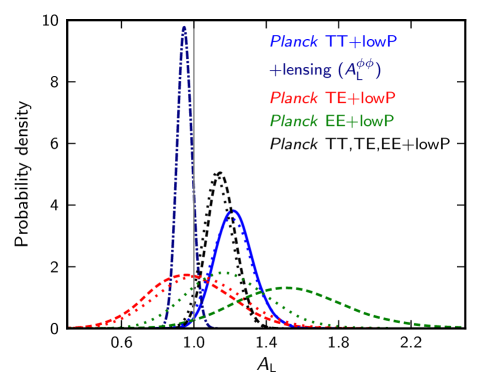
Given the precision of the measured compared to the uncertainty in the predicted spectrum from fits to the Planck TT+lowP data, the structure in the residuals seen in Fig. 11 might be expected to pull parameters in joint fits. As discussed in Planck Collaboration XV (2016) and Pan et al. (2014), the primary parameter dependence of at multipoles is through and in models. Here, is the angular multipole corresponding to the horizon size at matter-radiation equality observed at a distance . The combination determines the mean-squared deflection , while controls the shape of . For the parameter ranges of interest,
| (2) |
where arises (mostly) from the strong wavenumber dependence of the transfer function for the gravitational potential, with around .
In joint fits to Planck TT+lowP+lensing, the main parameter changes from Planck TT+lowP alone are a reduction in the best-fit , with an accompanying reduction in the best-fit , to (around ; see Sect. 3.4). There is also a reduction in , achieved at fixed by reducing . These combine to reduce by approximately at , consistent with Eq. (2). The difference between the theory lensing spectrum at the best-fit parameters in the Planck TT+lowP and Planck TT+lowP+lensing fits are shown by the dashed blue lines in Fig. 11. In the joint fit, the for the lensing bandpowers improves by 6, while the for the Planck TT+lowP data degrades by only ( for the high- data and for the low- data).
The lower values of and in the joint fit give a reduction in , with
| (3) |
as shown in Fig. 19. The decrease in matter density leads to a corresponding decrease in , and at fixed (approximately ) a increase in , giving
| (4) |
Joint Planck+lensing constraints on other parameters of the base cosmology are given in Table. 4.
Planck Collaboration XV (2016) discusses the effect on parameters of extending the lensing multipole range in joint fits with . In the base model, using the full multipole range , the parameter combination (which is well determined by the lensing measurements) is pulled around lower that its value using the conservative lensing range, with a negligible change in the uncertainty. Around half of this shift comes from the outlying bandpower (). In massive neutrino models, the total mass is similarly pulled higher by around when using the full lensing multipole range.
5.1.2 Detection of lensing in the CMB power spectra
The smoothing effect of lensing on the acoustic peaks and troughs of the power spectrum is detected at high significance in the Planck data. Following PCP13 (see also Calabrese et al. 2008), we introduce a parameter , which scales the theory power spectrum at each point in parameter space, and which is used to lens the CMB spectra.191919We emphasize the difference between the phenomenological parameters and (introduced earlier). The amplitude multiplies when calculating both the lensed CMB theory spectra and the lensing likelihood, while affects only the lensing likelihood by scaling the theory when comparing with the power spectrum of the reconstructed lensing potential . The expected value for base is . The results of such an analysis for models with variable is shown in Fig. 12. The marginalized constraint on is
| (5) |
This is very similar to the result from the 2013 Planck data reported in PCP13. The persistent preference for is discussed in detail there. For the 2015 data, we find that between the best-fitting model and the best-fitting base model. There is roughly equal preference for high from intermediate and high multipoles (i.e., the Plik likelihood; ) and from the low- likelihood (), with a further small change coming from the priors.
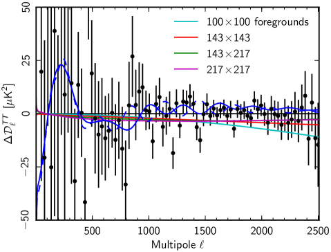
Increases in are accompanied by changes in all other parameters, with the general effect being to reduce the predicted CMB power on large scales, and in the region of the second acoustic peak, and to increase CMB power on small scales (see Fig. 13). A reduction in the high- foreground power compensates the CMB increase on small scales. Specifically, is increased by relative to the best-fitting base model and is reduced by , both of which lower the large-scale power to provide a better fit to the measured spectra around (see Fig. 1). The densities and respond to the change in , following the usual acoustic degeneracy, and falls by , attempting to reduce power in the damping tail due to the increase in and reduction in the diffusion angle (which follows from the reduction in ). The changes in and lead to a reduction in from to . With these cosmological parameters, the lensing power is lower than in the base model, which additionally increases the CMB power in the acoustic peaks and reduces it in the troughs. This provides a poor fit to the measured spectra around the fourth and fifth peaks, but this can be mitigated by increasing to give more smoothing from lensing than in the base model. However, further increases power in the damping tail, but this is partly offset by reduction of the power in the high- foregrounds.
The trends in the spectrum that favour high have a similar pull on parameters such as curvature (Sect. 6.2.4) and the dark energy equation of state (Sect. 6.3) in extended models. These parameters affect the late-time geometry and clustering and so alter the lensing power, but their effect on the primary CMB fluctuations is degenerate with changes in the Hubble constant (to preserve ). The same parameter changes as those in models are found in these extended models, but with, for example, the increase in replaced by a reduction in . Adding external data, however, such as the Planck lensing data or BAO (Sect. 5.2), pull these extended models back to base .
Finally, we note that lensing is also detected at lower significance in the polarization power spectra (see Fig. 12):
| (6a) | ||||
| (6b) | ||||
These results use only polarization at low multipoles, i.e., with no temperature data at multipoles . These are the first detections of lensing in the CMB polarization spectra, and reach almost in . We caution the reader that the constraints from and low- polarization are rather unstable between high- likelihoods because of differences in the treatment of the polarization data (see Fig. 12, which compares constraints from the Plik and CamSpec polarization likelihoods). The result of replacing Plik with the CamSpec likelihood is , i.e., around lower than the result from Plik reported in Eq. (6b). If we additionally include the low- temperature data, from increases:
| (7) |
The pull to higher in this case is due to the reduction in power in these models on large scales (as discussed above).
5.2 Baryon acoustic oscillations
Baryon acoustic oscillation (BAO) measurements are geometric and largely unaffected by uncertainties in the nonlinear evolution of the matter density field and additional systematic errors that may affect other types of astrophysical data. As in PCP13, we therefore use BAO as a primary astrophysical data set to break parameter degeneracies from CMB measurements.
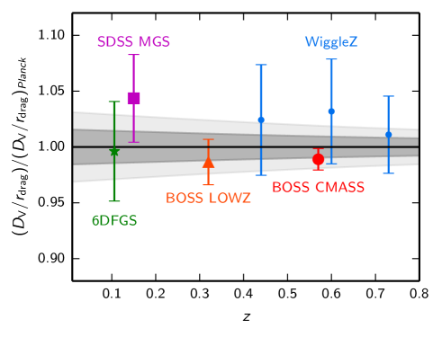
Figure 14 shows an updated version of figure 15 from PCP13. The plot shows the acoustic-scale distance ratio measured from a number of large-scale structure surveys with effective redshift , divided by the mean acoustic-scale ratio in the base cosmology using Planck TT+lowP+lensing. Here is the comoving sound horizon at the end of the baryon drag epoch and is a combination of the angular diameter distance and Hubble parameter ,
| (8) |
The grey bands in the figure show the and ranges allowed by Planck in the base cosmology.
The changes to the data points compared to figure 15 of PCP13 are as follows. We have replaced the SDSS DR7 measurements of Percival et al. (2010) with the recent analysis of the SDSS Main Galaxy Sample (MGS) of Ross et al. (2015) at , and by the Anderson et al. (2014) analysis of the Baryon Oscillation Spectroscopic Survey (BOSS) “LOWZ” sample at . Both of these analyses use peculiar velocity field reconstructions to sharpen the BAO feature and reduce the errors on . The blue points in Fig. 14 show a reanalysis of the WiggleZ redshift survey by Kazin et al. (2014) that applyies peculiar velocity reconstructions. These reconstructions cause small shifts in compared to the unreconstructed WiggleZ results of Blake et al. (2011) and lead to reductions in the errors on the distance measurements at and . The point labelled BOSS CMASS at shows from the analysis of Anderson et al. (2014), updating the BOSS-DR9 analysis of Anderson et al. (2012) used in PCP13.
In fact, the Anderson et al. (2014) analysis solves jointly for the positions of the BAO feature in both the line-of-sight and transverse directions (the distortion in the transverse direction caused by the background cosmology is sometimes called the Alcock-Paczynski effect, Alcock & Paczynski 1979), leading to joint constraints on the angular diameter distance and the Hubble parameter . These constraints, using the tabulated likelihood included in the CosmoMC module,202020http://www.sdss3.org/science/boss_publications.php are plotted in Fig. 15. Samples from the Planck TT+lowP+lensing chains are shown for comparison, coloured by the value of . The length of the degeneracy line is set by the allowed variation in (or equivalently ). In the Planck TT+lowP+lensing analysis the line is defined approximately by
| (9) |
which just grazes the BOSS CMASS 68 % error ellipse plotted in Fig. 15. Evidently, the Planck base parameters are in good agreement with both the isotropized BAO measurements plotted in Fig. 14, and with the anisotropic constraints plotted in Fig. 15.
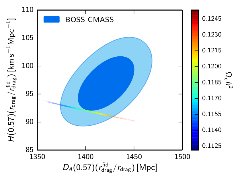
In this paper, we use the 6dFGS, SDSS-MGS, and BOSS-LOWZ BAO measurements of (Beutler et al. 2011; Ross et al. 2015; Anderson et al. 2014) and the CMASS-DR11 anisotropic BAO measurements of Anderson et al. (2014). Since the WiggleZ volume partially overlaps that of the BOSS-CMASS sample, and the correlations have not been quantified, we do not use the WiggleZ results in this paper. It is clear from Fig. 14 that the combined BAO likelihood is dominated by the two BOSS measurements.
In the base model, the Planck data constrain the Hubble constant and matter density to high precision:
| (10) |
With the addition of the BAO measurements, these constraints are strengthened significantly to
| (11) |
These numbers are consistent with the Planck+lensing constraints of Eq. (4). Section 5.4 discusses the consistency of these estimates of with direct measurements.
Although low-redshift BAO measurements are in good agreement with Planck for the base cosmology, this may not be true at high redshifts. Recently, BAO features have been measured in the flux-correlation function of the Ly forest of BOSS quasars (Delubac et al. 2015) and in the cross-correlation of the Ly forest with quasars (Font-Ribera et al. 2014). These observations give measurements of and (with somewhat lower precision) at and , respectively. For example, from table II of Aubourg et al. (2015) the two Ly BAO measurements combined give , compared to the predictions of the base Planck cosmology of , which are discrepant at the level. At present, it is not clear whether this discrepancy is caused by systematics in the Ly BAO measurements (which are more complex and less mature than galaxy BAO measurements) or an indicator of new physics. As Aubourg et al. (2015) discuss, it is difficult to find a physical explanation for the Ly BAO results without disrupting the consistency with the much more precise galaxy BAO measurements at lower redshifts.
5.3 Type Ia supernovae
Type Ia supernovae (SNe) are powerful probes of cosmology (Riess et al. 1998; Perlmutter et al. 1999) and particularly of the equation of state of dark energy. In PCP13, we used two samples of type Ia SNe, the “SNLS” compilation (Conley et al. 2011) and the “Union2.1” compilation (Suzuki et al. 2012). The SNLS sample was found to be in mild tension, at about the level, with the 2013 Planck base cosmology favouring a value of compared to the Planck value of . Another consequence of this tension showed up in extensions to the base model, where the combination of Planck and the SNLS sample showed evidence for a “phantom” () dark energy equation of state.
Following the submission of PCP13, Betoule et al. (2013) reported the results of an extensive campaign to improve the relative photometric calibrations between the SNLS and SDSS supernova surveys. The “Joint Light-curve Analysis” (JLA) sample, used in this paper, is constructed from the SNLS and SDSS SNe data, together with several samples of low redshift SNe.212121A CosmoMC likelihood model for the JLA sample is available at http://supernovae.in2p3.fr/sdss_snls_jla/ReadMe.html. The latest version in CosmoMC includes numerical integration over the nuisance parameters for use when calculating joint constraints using importance sampling; this can give different values compared to parameter best fits.. Cosmological constraints from the JLA sample are discussed by Betoule et al. (2014) and residual biases associated with the photometry and light curve fitting are assessed by Mosher et al. (2014). For the base cosmology, Betoule et al. (2014) find , consistent with the 2013 and 2015 Planck values for base . This relieves the tension between the SNLS and Planck data reported in PCP13. Given the consistency between Planck and the JLA sample for base , one can anticipate that the combination of these two data sets will constrain the dark energy equation of state to be close to (see Sect. 6.3).
Since the submission of PCP13, first results from a sample of Type Ia SNe discovered with the Pan-STARRS survey have been reported by Rest et al. (2014) and Scolnic et al. (2014). The Pan-STARRS sample is still relatively small (consisting of spectroscopically confirmed Type Ia SNe) and is not used in this paper.
5.4 The Hubble constant
CMB experiments provide indirect and highly model-dependent estimates of the Hubble constant. It is therefore important to compare CMB estimates with direct estimates of , since any significant evidence of a tension could indicate the need for new physics. In PCP13, we used the Riess et al. (2011, hereafter R11) Hubble Space Telescope (HST) Cepheid+SNe based estimate of as a supplementary “-prior.” This value was in tension at about the level with the 2013 Planck base value of .
For the base model, CMB and BAO experiments consistently find a value of lower than the R11 value. For example, the 9-year WMAP data (Bennett et al. 2013; Hinshaw et al. 2013) give:222222These numbers are taken from our parameter grid, which includes a neutrino mass of and the same updated BAO compilation as Eq. (11) (see Sect. 5.2).
| (0a) | |||||
| (0b) |
These numbers can be compared with the Planck 2015 values given in Eqs. (10) and (11). The WMAP constraints are driven towards the Planck values by the addition of the BAO data and so there is persuasive evidence for a low in the base cosmology independently of the high-multipole CMB results from Planck. The 2015 Planck TT+lowP value is entirely consistent with the 2013 Planck value and so the tension with the R11 determination remains at about .
The tight constraint on in Eq. (0b) is an example of an “inverse distance ladder,” where the CMB primarily constrains the sound horizon within a given cosmology, providing an absolute calibration of the BAO acoustic-scale (e.g., Percival et al. 2010; Cuesta et al. 2015; Aubourg et al. 2015, see also PCP13). In fact, in a recent paper Aubourg et al. (2015) use the 2013 Planck constraints on in combination with BAO and the JLA SNe data to find , in excellent agreement with the 2015 Planck value for base given in Eq. (10), which is based on the Planck temperature power spectrum. Note that by adding SNe data, the Aubourg et al. (2015) estimate of is insensitive to spatial curvature and to late time variations of the dark energy equation of state. Evidently, there are a number of lines of evidence that point to a lower value of than the direct determination of R11.
The R11 Cepheid data have been reanalysed by Efstathiou (2014, hereafter E14) using the revised geometric maser distance to NGC 4258 of Humphreys et al. (2013). Using NGC 4258 as a distance anchor, E14 finds
| (1) |
which is within of the Planck TT estimate given in Eq. (10). In this paper we use Eq. (1) as a “conservative” prior.
R11 also use Large Magellanic Cloud Cepheids and a small sample of Milky Way Cepheids with parallax distances as alternative distance anchors to NGC4258. The R11 prior used in PCP13 combines all three distance anchors. Combining the LMC and MW distance anchors, E14 finds
| (2) |
under the assumption that there is no metallicity variation of the Cepheid period-luminosity relation. This is discrepant with Eq. (10) at about the level. However, neither the central value nor the error in Eq. (2) is reliable. The MW Cepheid sample is small and dominated by short period () objects. The MW Cepheid sample therefore has very little overlap with the period range of SNe host galaxy Cepheids observed with HST. As a result, the MW solutions for are unstable (see Appendix A of E14). The LMC solution is sensitive to the metallicity dependence of the Cepheid period-luminosity relation which is poorly constrained by the R11 data. Furthermore, the estimate in Eq. (1) is based on a differential measurement, comparing HST photometry of Cepheids in NGC 4258 with those in SNe host galaxies. It is therefore less prone to photometric systematics, such as crowding corrections, than is the LMC+MW estimate of Eq. (2). It is for these reasons that we have adopted the prior of Eq. (1) in preference to using the LMC and MW distance anchors.232323As this paper was nearing completion, results from the Nearby Supernova Factory have been presented that indicate a correlation between the peak brightness of Type Ia SNe and the local star-formation rate (Rigault et al. 2015). These authors argue that this correlation introduces a systematic bias of around in the SNe/Cepheid distance scale measurement of . For example, according to these authors, the estimate of Eq. (1) should be lowered to , a downward shift of approximately . Clearly, further work needs to be done to assess the importance of such a bias on the distance scale. It is ignored in the rest of this paper.
Direct measurements of the Hubble constant have a long and sometimes contentious history (see, e.g., Tammann et al. 2008). The controversy continues to this day and in the literature one can find “high” values, e.g., (Freedman et al. 2012), and “low” values, e.g., (Tammann & Reindl 2013). The key point that we wish to make is that the Planck-only estimates of Eqs. (4) and (10), and the Planck+BAO estimate of Eq. (11) all have small errors and are consistent. If a persuasive case can be made that a direct measurement of conflicts with these estimates, then this will be strong evidence for additional physics beyond the base model.
Finally, we note that in a recent analysis Bennett et al. (2014) derive a “concordance” value of for base by combining WMAP9+SPT+ACT+BAO with a slightly revised version of the R11 value, . The Bennett et al. (2014) central value for differs from the Planck value of Eq. (11) by nearly (or ). The reason for this difference is that the Planck data are in tension with the Story et al. (2013) SPT data (as discussed in Appendix B of PCP13; note that the tension is increased with the Planck full mission data) and with the revised R11 determination. Both tensions drive the Bennett et al. (2014) value of away from the Planck solution.
5.5 Additional data
5.5.1 Redshift space distortions
Transverse versus line-of-sight anisotropies in the redshift-space clustering of galaxies induced by peculiar motions can, potentially, provide a powerful way of constraining the growth rate of structure (e.g., Percival & White 2009). A number of studies of redshift-space distortions (RSD) have been conducted to measure the parameter combination , where for models with scale-independent growth
| (3) |
and is the linear growth rate of matter fluctuations. Notice that the parameter combination is insensitive to differences between the clustering of galaxies and dark matter, i.e., to galaxy bias (Song & Percival 2009). In the base cosmology, the growth factor is well approximated as . More directly, in linear theory the quadrupole of the redshift-space clustering anisotropy actually probes the density-velocity correlation power spectrum, and we therefore define
| (4) |
as an approximate proxy for the quantity actually being measured. Here measures the smoothed density-velocity correlation and is defined analogously to , but using the correlation power spectrum , where and is the Newtonian-gauge (peculiar) velocity of the baryons and dark matter, and is the total matter density perturbation. This definition assumes that the observed galaxies follow the flow of the cold matter, not including massive neutrino velocity effects. For models close to , where the growth is nearly scale independent, it is equivalent to defining in terms of the growth of the baryon+CDM density perturbations (excluding neutrinos).
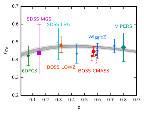
The use of RSD as a measure of the growth of structure is still under active development and is considerably more difficult than measuring the positions of BAO features. Firstly, adopting the wrong fiducial cosmology can induce an anisotropy in the clustering of galaxies, via the Alcock-Paczynski (AP) effect, which is strongly degenerate with the anisotropy induced by peculiar motions. Secondly, much of the RSD signal currently comes from scales where nonlinear effects and galaxy bias are significant and must be accurately modelled in order to relate the density and velocity fields (see, e.g., the discussions in Bianchi et al. 2012; Okumura et al. 2012; Reid et al. 2014; White et al. 2015).
Current constraints,242424The constraint of Chuang et al. (2013) plotted in the original version of this paper was subsequently shown to be in error. We therefore now show updated BOSS data points for DR12 from Chuang et al. (2013, for CMASS) and Gil-Marín et al. (2015, for LOWZ). assuming a Planck base model, are shown in Fig. 16. Neglecting the AP effect can lead to biased measurements of if the assumed cosmology differs, and to significant underestimation of the errors (Howlett et al. 2015). The analyses summarized in Fig. 16 solve simultaneously for RSD and the AP effect, except for the 6dFGS point (which is insensitive to cosmology) and the VIPERS point (which has a large error). The grey bands show the range allowed by Planck TT+lowP+lensing in the base model, and are consistent with the RSD data. The tightest constraints on in this figure come from the BOSS CMASS-DR11 analyses of Beutler et al. (2014) and Samushia et al. (2014). The Beutler et al. (2014) analysis is performed in Fourier space and shows a small bias in compared to numerical simulations when fitting over the wavenumber range 0.01–. The Samushia et al. (2014) analysis is performed in configuration space and shows no evidence of biases when compared to numerical simulations. The updated DR12 CMASS result from Chuang et al. (2013) marginalizes over a polynomial model for systematic errors in the correlation function monopole, and is consistent with these and the Planck constraints, with a somewhat larger error bar.
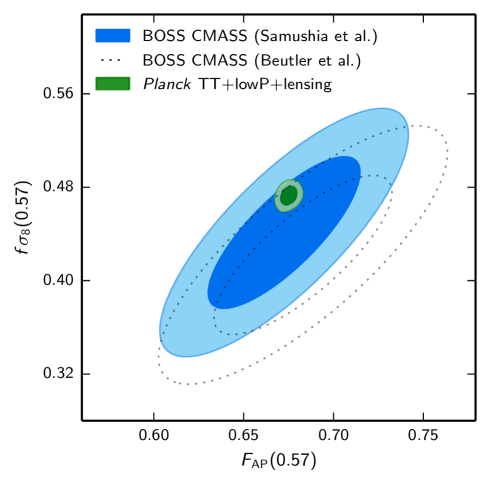
The Samushia et al. (2014) results are expressed as a covariance matrix for the three parameters , and , evaluated at an effective redshift of , where is the “Alcock-Paczynski” parameter
| (5) |
The principal degeneracy is between and and is illustrated in Fig. 17, compared to the constraint from Planck TT+lowP+lensing for the base cosmology. The Planck results sit slightly high but overlap the contour from Samushia et al. (2014). The Planck result lies about higher than the Beutler et al. (2014) analysis of the BOSS CMASS sample.
RSD measurements are not used in combination with Planck in this paper. However, in the companion paper exploring dark energy and modified gravity (Planck Collaboration XIV 2016), the RSD/BAO measurements of Samushia et al. (2014) are used together with Planck. Where this is done, we exclude the Anderson et al. (2014) BOSS-CMASS results from the BAO likelihood. Since Samushia et al. (2014) do not apply a density field reconstruction in their analysis, the BAO constraints from BOSS-CMASS are then slightly weaker, though consistent, with those of Anderson et al. (2014).
5.5.2 Weak gravitational lensing
Weak gravitational lensing offers a potentially powerful technique for measuring the amplitude of the matter fluctuation spectrum at low redshifts. Currently, the largest weak lensing data set is provided by the CFHTLenS survey (Heymans et al. 2012; Erben et al. 2013). The first science results from this survey appeared shortly before the completion of PCP13 and it was not possible to do much more than offer a cursory comparison with the Planck 2013 results. As reported in PCP13, at face value the results from CFHTLenS appeared to be in tension with the Planck 2013 base cosmology at about the 2– level. Since neither the CFHTLenS results nor the 2015 Planck results have changed significantly from those in PCP13, it is worth discussing this discrepancy in more detail in this paper.
Weak lensing data can be analysed in various ways. For example, one can compute two correlation functions from the ellipticities of pairs of images separated by angle ,which are related to the convergence power spectrum of the survey at multipole via
| (6) |
where the Bessel functions in (6) are and (see, e.g., Bartelmann & Schneider 2001). Much of the information from the CFHTLenS survey correlation function analyses comes from wavenumbers at which the matter power spectrum is strongly nonlinear, complicating any direct comparison with Planck.
This can be circumventing by performing a 3D spherical harmonic analysis of the shear field, allowing one to impose lower limits on the wavenumbers that contribute to a weak lensing likelihood. This has been done by Kitching et al. (2014). Including only wavenumbers with , Kitching et al. (2014) find constraints in the – plane that are consistent with the results from Planck. However, by excluding modes with higher wavenumbers, the lensing constraints are weakened. When they increase the wavenumber cut-off to some tension with Planck begins to emerge (which these authors argue may be an indication of the effects of baryonic feedback in suppressing the matter power spectrum at small scales). The large-scale properties of CFHTLenS therefore seem broadly consistent with Planck and it is only as CFHTLenS probes higher wavenumbers, particular in the 2D and tomographic correlation function analyses (Heymans et al. 2013; Kilbinger et al. 2013; Fu et al. 2014; MacCrann et al. 2015), that apparently strong discrepancies with Planck appear.
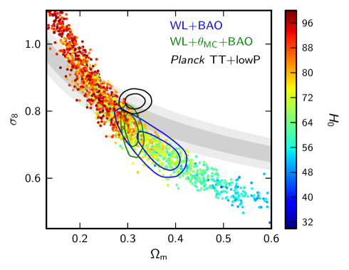
The situation is summarized in Fig. 18. The sample points show parameter values in the – plane for the base model, computed from the Heymans et al. (2013, hereafter H13) tomographic measurements of . These data consist of correlation function measurements in six photometric redshift bins extending over the redshift range 0.2–1.3. We use the blue galaxy sample, since H13 find that this sample shows no evidence for intrinsic galaxy alignments (simplifying the comparison with theory) and we apply the “conservative” cuts of H13, intended to reduce sensitivity to the nonlinear part of the power spectrum; these cuts eliminate measurements with for any redshift combination that involves the lowest two redshift bins. Here we have used the halofit prescription of Takahashi et al. (2012) to model the nonlinear power spectrum, but do not include any model of baryon feedback or intrinsic alignments. For the lensing-only constraint we also impose additional priors in a similar way to the CMB lensing analysis described in Planck Collaboration XV (2016), i.e., Gaussian priors and , where the exact values (chosen to span reasonable ranges given CMB data) have little impact on the results. The sample range shown also restricts the Hubble parameter to ; note that when comparing with constraint contours, the location of the contours can change significantly depending on the prior range assumed. We also use a weak prior on the primoridal amplitude, , which shows up the strong correlation between –– in the region of parameter space relevant for comparison with Planck. In Fig. 18 we only show lensing contours after the samples have been projected into the space allowed by the BAO data (blue contours), or also additionally restricting to the reduced space where is fixed to the Planck value, which is accurately measured. The black contours show the constraints from Planck TT+lowP.
The lensing samples just overlap with Planck, and superficially one might conclude that the two data sets are consistent. However, the weak lensing constraints approximately define a 1D degeneracy in the 3D –– space, so consistency of the Hubble parameter at each point in the projected space must also be considered (see appendix E1 of Planck Collaboration XV 2016). Comparing the contours in Fig. 18 (the regions where the weak lensing constraints are consistent with BAO observations) the CFHTLenS data favour a lower value of than the Planck data (and much of the area of the blue contours also has higher ). However, even with the conservative angular cuts applied by H13, the weak lensing constraints depend on the nonlinear model of the power spectrum and on the possible influence of baryonic feedback in reshaping the matter power spectrum at small spatial scales (Harnois-Déraps et al. 2015; MacCrann et al. 2015). The importance of these effects can be reduced by imposing even more conservative angular cuts on , but of course, this weakens the statistical power of the weak lensing data. The CFHTLenS data are not used in combination with Planck in this paper (apart from specific cases in Sects. 6.3 and 6.4.4) and, in any case, would have little impact on most of the extended constraints discussed in Sect. 6. Weak lensing can, however, provide important constraints on dark energy and modified gravity. The CFHTLenS data are therefore used in combination with Planck in the companion paper (Planck Collaboration XIV 2016), which explores several halofit prescriptions and the impact of applying more conservative angular cuts to the H13 measurements.
5.5.3 Planck cluster counts
In 2013 we noted a possible tension between our primary CMB constraints and those from the Planck SZ cluster counts, with the clusters preferring lower values of in the base CDM model in some analyses (Planck Collaboration XX 2014). The comparison is interesting because the cluster counts directly measure at low redshift; any tension could signal the need for extensions to the base model, such as non-minimal neutrino mass (though see Sect. 6.4). However, limited knowledge of the scaling relation between SZ signal and mass have hampered the interpretation of this result.
With the full mission data we have created a larger catalogue of SZ clusters with a more accurate characterization of its completeness (Planck Collaboration XXIV 2016). By fitting the counts in redshift and signal-to-noise, we are able to simultaneously constrain the slope of the SZ signal–mass scaling relation and the cosmological parameters. A major uncertainty, however, remains the overall mass calibration, which in Planck Collaboration XX (2014) we quantified with a “hydrostatic bias” parameter, , with a fiducial value of and a range (consistent with some other studies, e.g., Simet et al. 2015). In the base model, the primary CMB constraints prefer a normalization below the lower end of this range, . The recent, empirical normalization of the relation by the Weighing the Giants lensing programme (WtG; von der Linden et al. 2014) gives for the 22 clusters in common with the Planck cluster sample. This calibration reduces the tension with the primary CMB constraints in base . In contrast, correlating the entire Planck 2015 SZ cosmology sample with Planck CMB lensing gives (Planck Collaboration XXIV 2016), toward the upper end of the range adopted in Planck Collaboration XX (2014), although with a large uncertainty. An alternative lensing calibration analysis by the Canadian Cluster Comparison Project, which uses 37 clusters in common with the Planck cluster sample (Hoekstra et al. 2015) finds , which lies between the other two mass calibrations. These calibrations are not yet definitive and the situation will continue to evolve with improvements in mass measurements from larger samples of clusters.
A recent analysis of cluster counts for an X-ray-selected sample (REFLEX II) shows some tension with the Planck base cosmology (Böhringer et al. 2014). However, an analysis of cluster counts of X-ray-selected clusters by the WtG collaboration, incorporating the WtG weak lensing mass calibration, finds , in good agreement with the Planck CMB results for base (Mantz et al. 2015). This raises the possibility that there may be systematic biases in the assumed scaling relations for SZ-selected clusters compared to X-ray-selected clusters (in addition to a possible mass calibration bias). Mantz et al. (2015) give a brief review of recent determinations of from X-ray, optically-selected, and SZ-selected samples, to which we refer the reader. More detailed discussion of constraints from combining Planck cluster counts with primary CMB anisotropies and other data sets can be found in Planck Collaboration XXIV (2016).
5.6 Cosmic concordance?
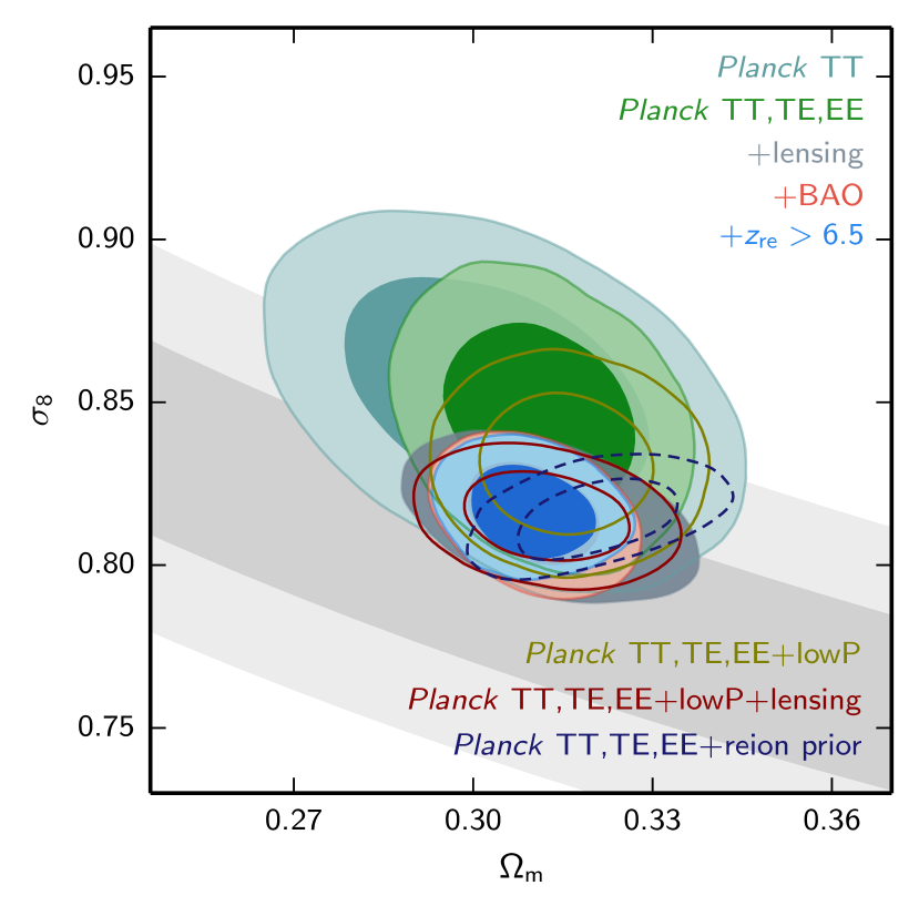
Table 4 summarizes the cosmological parameters in the base for Planck combined with various data sets discussed in this section. Although we have seen from the survey presented above that base is consistent with a wide range of cosmological data, there are two areas of tension:
The first point to note is that the astrophysical data in areas (1) and (2) are complex and more difficult to interpret than most of the astrophysical data sets discussed in this section. The interpretation of the data in area (2) depends on nonlinear modelling of the power spectrum, and in the case of clusters and weak lensing, on uncertain baryonic physics. Understanding these effects more accurately sets a direction for future research.
It is, however, worth reviewing our findings on and from Planck assuming base . These are summarized in Fig. 19 and the following constraints:
| (0a) | |||||
| (0b) | |||||
| (0c) |
The last line imposes a Gaussian prior of with a limit on the reionization redshift in place of the reionization constraints from the lowP likelihood. As discussed in Sect. 3.4, such a low redshift of reionization is close to the lowest plausible value allowed by astrophysical data (though such low values are not favoured by either the WMAP or LFI polarization data). The addition of Planck lensing data pulls down by about from the Planck TT+lowP value, so Eq. (0c) is the lowest possible range allowed by the Planck CMB data. As shown in Fig. 19, adding the and spectra at high multipoles does not change the Planck constraints. If a convincing case can be made that astrophysical data conflict with the estimate of Eq. (0c), then this will be powerful evidence for new physics beyond base with minimal-mass neutrinos.
A number of authors have interpreted the discrepancies in area (2) as evidence for new physics in the neutrino sector (e.g., Planck Collaboration XX 2014; Hamann & Hasenkamp 2013; Battye & Moss 2014; Battye et al. 2015; Wyman et al. 2014; Beutler et al. 2014). They use various data combinations together with Planck to argue for massive neutrinos with mass or for a single sterile neutrino with somewhat higher mass. The problem here is that any evidence for new neutrino physics is driven mainly by the additional astrophysical data, not by Planck CMB anisotropy measurements. In addition, the external data sets are not entirely consistent, so tensions remain. As discussed in PCP13 (see also Leistedt et al. 2014; Battye et al. 2015) Planck data usually favour base over extended models. Implications of the Planck 2015 data for neutrino physics are discussed in Sect. 6.4 and tensions between Planck and external data in various extended neutrino models are discussed further in Sect. 6.4.4.
As mentioned above, we do not use RSD or galaxy weak lensing measurements for combined constraints in this paper (apart from Sects. 6.3 and 6.4.4, where we use the CFHTLenS data) . They are, however, used in the paper exploring constraints on dark energy and modified gravity (Planck Collaboration XIV 2016). For some models discussed in that paper, the combination of Planck, RSD, and weak lensing data does prefer extensions to the base cosmology.
|
6 Extensions to the base CDM model
| Parameter . . . . . . . |
6.1 Grid of models
The full grid results are available online.252525See the Planck Legacy Archive, http://www.cosmos.esa.int/web/planck/pla, which contains considerably more detailed information than presented in this paper. Figure 20 and Table 5 summarize the constraints on one-parameter extensions to base . As in PCP13, we find no strong evidence in favour of any of these simple one-parameter extensions using Planck or Planck combined with BAO. The entire grid has been run using both the Plik and CamSpec likelihoods. As noted in Sect. 3, the parameters derived from these two likelihoods agree to better than for base . This level of agreement also holds for the extended models analysed in our grid. In Sect. 3 we also pointed out that we have definite evidence, by comparing spectra computed with different frequency combinations, of residual systematics in the and spectra. These systematics average down in the coadded and spectra, but the remaining level of systematics in these coadded spectra are not yet well quantified (though they are small). Thus, we urge the reader to treat parameters computed from the TT,TE,EE likelihoods with some caution. In the case of polarization, the agreement between the Plik and CamSpec and likelihoods is less good, with shifts in parameters of up to (though such large shifts are unusual). In general, the behaviour of the TT,TE,EE likelihoods is as shown in Fig. 20. For extended models, the addition of the Planck polarization data at high multipoles reduces the errors on extended parameters compared to the Planck temperature data and pulls the parameters towards those of base . A similar behaviour is seen if the Planck TT (or Planck TT,TE,EE) data are combined with BAO.
The rest of this section discusses the grid results in more detail and also reports results on some additional models (specifically dark matter annihilation, tests of the recombination history, and cosmic defects) that are not included in our grid.
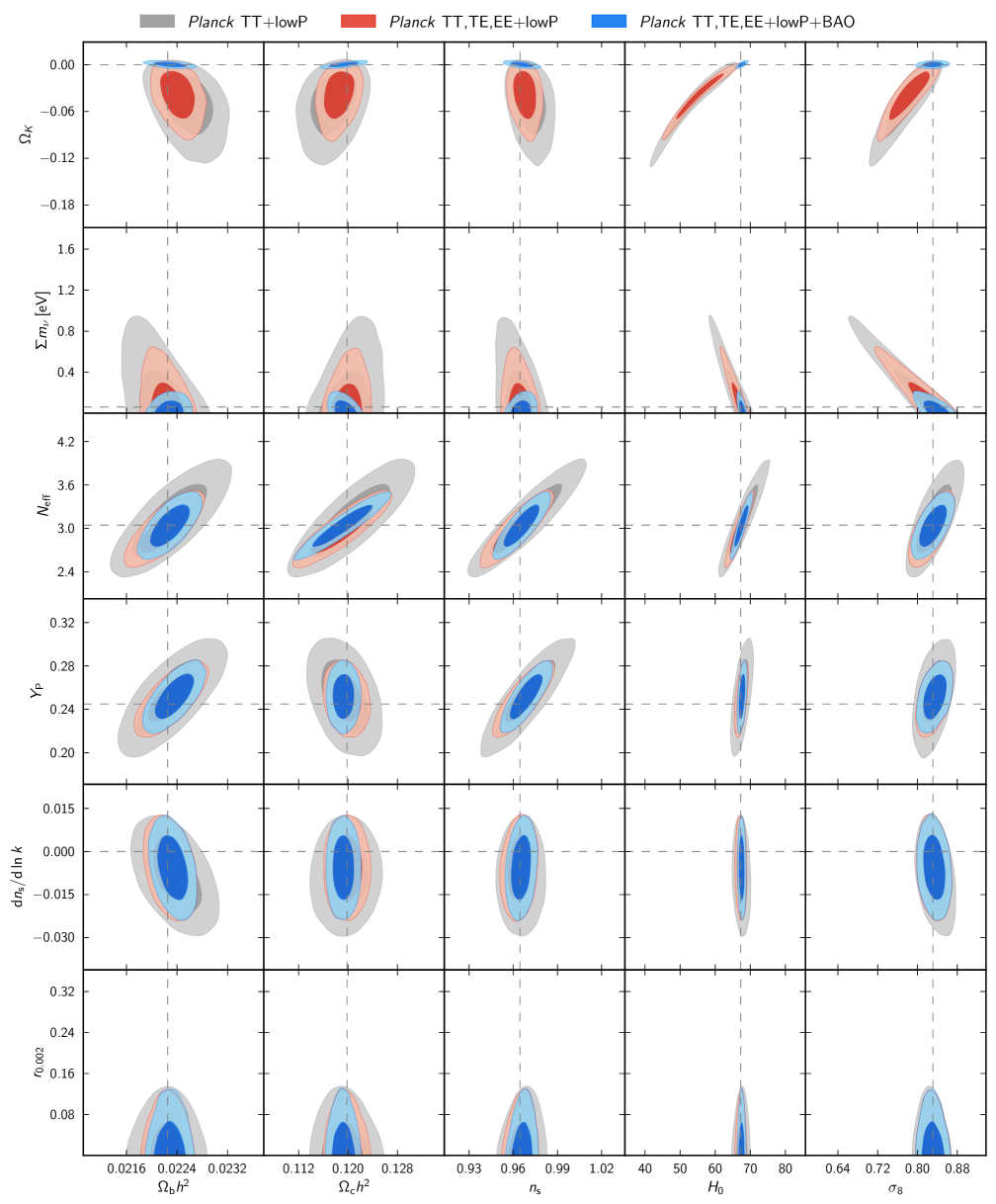
6.2 Early-Universe physics
Arguably the most important result from 2013 Planck analysis was the finding that simple single-field inflationary models, with a tilted scalar spectrum , provide a very good fit to the Planck data. We found no evidence for a tensor component or running of the scalar spectral index, no strong evidence for isocurvature perturbations or features in the primordial power spectrum (Planck Collaboration XXII 2014), and no evidence for non-Gaussianity (Planck Collaboration XXIV 2014), cosmic strings or other topological defects (Planck Collaboration XXV 2014). On large angular scales, the Planck data showed some evidence for “anomalies” seen previously in the WMAP data (Bennett et al. 2011). These include a dip in the power spectrum in the multipole range (see Fig. 1) and some evidence for a departure from statistical isotropy on large angular scales (Planck Collaboration XXIII 2014). However, the statistical significance of these anomalies is not high enough to provide compelling evidence for new physics beyond simple single-field inflation.
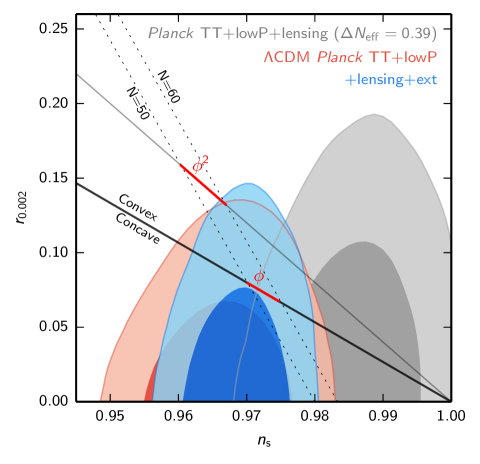
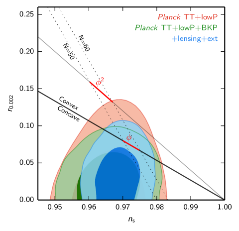
The Planck 2013 results led to renewed interest in the inflationary model, originally introduced by Starobinsky (1980), and related inflationary models that have flat effective potentials of similar form (e.g., Kallosh & Linde 2013; Ferrara et al. 2013; Buchmuller et al. 2013; Ellis et al. 2013). A characteristic of these models is that they produce a red tilted scalar spectrum and a low tensor-to-scalar ratio. For reference, the Starobinsky model predicts
| (0a) | |||||
| (0b) | |||||
| (0c) |
where is the number of e-foldings between the end of inflation and the time that our present day Hubble scale crossed the inflationary horizon, and numerical values are for the range .
Although the Planck 2013 results stimulated theoretical work on inflationary models with low tensor-to-scalar ratios, the cosmological landscape became more complicated following the detection of a -mode polarization anisotropy by the BICEP2 team (BICEP2 Collaboration 2014). If the BICEP2 signal were primarily caused by primordial gravitational waves, then the inferred tensor-to-scalar ratio would have been ,262626The pivot scale quoted here is roughly appropriate for the multipoles probed by BICEP2. apparently in conflict with the 2013 Planck 95 % upper limit of , based on fits to the temperature power spectrum. Since the Planck constraints on are highly model dependent (and fixed mainly by lower ) it is possible to reconcile these results by introducing additional parameters, such as large tilts or strong running of the spectral indices.
The situation has been clarified following a joint analysis of BICEP2/Keck observations and Planck polarization data reported in BKP. This analysis shows that polarized dust emission contributes a significant part of the BICEP2 signal. Correcting for polarized dust emission, BKP report a 95 % upper limit of on scale-invariant tensor modes, eliminating the tension between the BICEP2 and the Planck 2013 results. There is therefore no evidence for inflationary tensor modes from -mode polarization measurements at this time (although the BKP analysis leaves open the possibility of a much higher tensor-to-scalar ratio than the prediction of Eq. 0b for Starobinsky-type models).
The layout of the rest of this subsection is as follows. In Sect. 6.2.1 we review the Planck 2015 and Planck+BKP constraints on and . Constraints on the running of the scalar spectral index are presented in Sect. 6.2.2. Polarization data provide a powerful way of testing for isocurvature modes, as discussed in Sect. 6.2.3. Finally, Sect. 6.2.4 summarizes our results on spatial curvature. A discussion of specific inflationary models and tests for features in the primordial power spectrum can be found in Planck Collaboration XX (2016).
6.2.1 Scalar spectral index and tensor fluctuations
Primordial tensor fluctuations (gravitational waves) contribute to both the CMB temperature and polarization power spectra. Gravitational waves entering the horizon between recombination and the present day generate a tensor contribution to the large-scale CMB temperature anisotropy. In this data release, the strongest constraint on tensor modes from Planck data still comes from the CMB temperature spectrum at . The corresponding comoving wavenumbers probed by the Planck temperature spectrum have , with very little sensitivity to higher wavenumbers because gravitational waves decay on sub-horizon scales. The precision of the Planck constraint is limited by cosmic variance of the large-scale anisotropies (which are dominated by the scalar component), and it is also model dependent. In polarization, in addition to -modes, the and spectra also contain a signal from tensor modes coming from the last-scattering and reionization epochs. However, in this release the addition of Planck polarization constraints at do not significantly change the results from temperature and low- polarization (see Table 5).
Figure 21 shows the 2015 Planck constraint in the – plane, adding as a 1-parameter extension to base . For base (), the value of is
| (1) |
We highlight this number here since , a key parameter for inflationary cosmology, shows one of the largest shifts of any parameter in base between the Planck 2013 and Planck 2015 analyses (about ). As explained in Sect. 3.1, part of this shift was caused by the systematic in the nominal-mission spectrum used in PCP13.
The red contours in Fig. 21 show the constraints from Planck TT+lowP. These are similar to the constraints shown in Fig. 23 of PCP13, but with shifted to slightly higher values. The addition of BAO or the Planck lensing data to Planck TT+lowP lowers the value of , which, at fixed , increases the small-scale CMB power. To maintain the fit to the Planck temperature power spectrum for models with , these parameter shifts are compensated by a change in the amplitude and the tilt (by about ). The increase in to match the observed power on small scales leads to a decrease in the scalar power on large scales, allowing room for a slightly larger contribution from tensor modes. The constraints shown by the blue contours in Fig. 21, which combine Planck lensing, BAO, and other astrophysical data, are therefore tighter in the direction and shifted to slightly higher values, but marginally weaker in the -direction. The 95 % limits on are
| (0a) | |||||
| (0b) |
consistent with the results reported in PCP13. Here we assume the second-order slow-roll consistency relation for the tensor spectral index. The result in Eqs. (0a) and (0b) are mildly scale dependent, with equivalent limits on being weaker by about .
PCP13 noted a mismatch between the best-fit base model and the temperature power spectrum at multipoles , partly driven by the dip in the multipole range . If this mismatch is simply a statistical fluctuation of the model (and there is no compelling evidence to think otherwise), the strong Planck limit (compared to forecasts) is the result of chance low levels of scalar mode confusion. On the other hand, if the dip represents a failure of the model, the limits of Eqs. (0a) and (0b) may be underestimates. These issues are considered at greater length in Planck Collaboration XX (2016) and will not be discussed further in this paper.
As mentioned above, the Planck temperature constraints on are model-dependent and extensions to can give significantly different results. For example, extra relativistic degrees of freedom increase the small-scale damping of the CMB anisotropies at a fixed angular scale, which can be compensated by increasing , allowing a larger tensor mode. This is illustrated by the grey contours in Fig. 21, which show the constraints for a model with . Although this value of is disfavoured by the Planck data (see Sect. 6.4.1) it is not excluded at a high significance level.
This example emphasizes the need for direct tests of tensor modes based on measurements of a large-scale -mode pattern in CMB polarization. Planck -mode constraints from the 100- and 143-GHz HFI channels, presented in Planck Collaboration XI (2016), give a 95 % upper limit of . However, at present the tightest -mode constraints on come from the BKP analysis of the BICEP2/Keck field, which covers approximately centred on , .. These measurements probe the peak of the -mode power spectrum at around , corresponding to gravitational waves with that enter the horizon during recombination (i.e., somewhat smaller than the scales that contribute to the Planck temperature constraints on ). The results of BKP give a posterior for that peaks at , but is consistent with . Thus, at present there is no convincing evidence of a primordial -mode signal. At these low values of , there is no longer any tension with Planck temperature constraints.
The analysis of BKP constrains defined relative to a fixed fiducial -mode spectrum, and on its own does not give a useful constraint on either the scalar amplitude or . A combined analysis of the Planck CMB spectra and the BKP likelihood can, self-consistently, give constraints in the – plane, as shown in the right-hand panel of Fig. 21. The BKP likelihood pulls the contours to slightly non-zero values of , with best fits of around , but at very low levels of statistical significance. The BKP likelihood also rules out the upper tail of values allowed by Planck alone. The joint Planck+BKP likelihood analyses give the upper limits
| (0a) | |||||
| (0b) |
The exact values of these upper limits are weakly dependent on the details of the foreground modelling applied in the BKP analysis (see BKP for further details). The results given here are for the baseline 2-parameter model, varying the -mode dust amplitude and frequency scaling, using the lowest five -mode bandpowers.
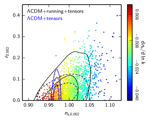
Allowing a running of the scalar spectral index as an additional free parameter weakens the Planck constraints on , as shown in Fig. 22. The coloured samples in Fig. 22 illustrate how a negative running allows the large-scale scalar spectral index to shift towards higher values, lowering the scalar power on large scales relative to small scales, thereby allowing a larger tensor contribution. However adding the BKP likelihood, which directly constrains the tensor amplitude on smaller scales, significantly reduces the extent of this degeneracy leading to a upper limit of even in the presence of running (i.e., similar to the results of Eqs. 0a and 0b).
The Planck+BKP joint analysis rules out a quadratic inflationary potential (, predicting ) at over 99 % confidence and reduces the allowed range of the parameter space for models with convex potentials. Starobinsky-type models are an example of a wider class of inflationary theories in which is not a coincidence, yet (Roest 2014; Creminelli et al. 2015). These models have concave potentials, and include a variety of string-inspired models with exponential potentials. Models with are, however, still allowed by the data, including a simple linear potential and fractional-power monomials, as well as regions of parameter space in between where is just a coincidence. Models that have sub-Planckian field evolution, so satisfying the Lyth bound (Lyth 1997; Garcia-Bellido et al. 2014), will typically have for , and are also consistent with the tensor constraints shown in Fig. 21. For further discussion of the implications of the Planck 2015 data for a wide range of inflationary models see Planck Collaboration XX (2016).
In summary, the Planck limits on are consistent with the BKP limits from -mode measurements. Both data sets are consistent with ; however, the combined data sets yield an upper limit to the tensor-to-scalar ratio of at the 95 % level. The Planck temperature constraints on are limited by cosmic variance. The only way of improving these limits, or potentially detecting gravitational waves with , is through direct -mode detection. The Planck 353-GHz polarization maps (Planck Collaboration Int. XXX 2016) show that at frequencies of around 150 GHz, Galactic dust emission is an important contaminant at the level even in the cleanest regions of the sky. BKP demonstrates further that on small regions of the sky covering a few hundred square degrees (typical of ground based -mode experiments), the Planck 353-GHz maps are of limited use as monitors of polarized Galactic dust emission because of their low signal-to-noise level. To achieve limits substantially below will require observations of comparably high sensitivity over a range of frequencies, and with increased sky coverage. The forthcoming measurements from Keck Array and BICEP3 at 95 GHz and the Keck Array receivers at 220 GHz should offer significant improvements on the current constraints. A number of other ground-based and sub-orbital experiments should also return high precision -mode data within the next few years (see Abazajian et al. 2015a, for a review).
6.2.2 Scale dependence of primordial fluctuations
In simple single-field models of inflation, the running of the spectral index is of second order in inflationary slow-roll parameters and is typically small, (Kosowsky & Turner 1995). Nevertheless, it is possible to construct models that produce a large running over a wavenumber range accessible to CMB experiments, whilst simultaneously achieving enough e-folds of inflation to solve the horizon problem. Inflation with an oscillatory potential of sufficiently long period, perhaps related to axion monodromy, is an example (Silverstein & Westphal 2008; Meerburg 2014; Czerny et al. 2014; Minor & Kaplinghat 2015).
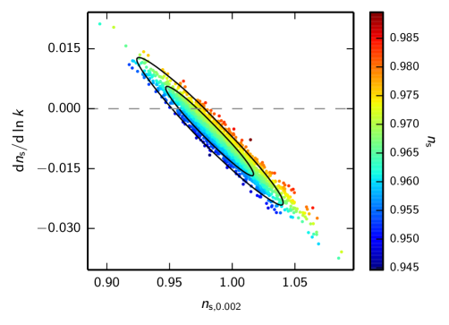
As reviewed in PCP13, previous CMB experiments, either on their own or in combination with other astrophysical data, have sometimes given hints of a non-zero running at about the level (Spergel et al. 2003; Hinshaw et al. 2013; Hou et al. 2014). The results of PCP13 showed a slight preference for negative running at the level, driven almost entirely by the mismatch between the CMB temperature power spectrum at high multipoles and the spectrum at multipoles .
The 2015 Planck results (Fig. 23) are similar to those in PCP13. Adding running as an additional parameter to base with , we find
| (0a) | |||||
| (0b) |
There is a slight preference for negative running, which, as in PCP13, is driven by the mismatch between the high and low multipoles in the temperature power spectrum. However, in the 2015 Planck data the tension between high and low multipoles is reduced somewhat, primarily because of changes to the HFI beams at multipoles (see Sect. 3.1). A consequence of this reduced tension can be seen in the 2015 constraints on models that include tensor fluctuations in addition to running:
| (0a) | |||||
| (0b) | |||||
| (0c) | |||||
PCP13 found an approximately pull towards negative running for these models. This tension is reduced to about with the 2015 Planck data, and to lower values when we include the BKP likelihood, which reduces the range of allowed tensor amplitudes.
In summary, the Planck data are consistent with zero running of the scalar spectral index. However, as illustrated in Fig. 23, the Planck data still allow running at roughly the level, i.e., an order of magnitude higher than expected in simple inflationary models. One way of potentially improving these constraints is to extend the wavenumber range from CMB scales to smaller scales using additional astrophysical data, for example by using measurements of the Ly flux power spectrum of high-redshift quasars (as in the first year WMAP analysis, Spergel et al. 2003). Palanque-Delabrouille et al. (2015) have recently reported an analysis of a large sample of quasar spectra from the SDSSIII/BOSS survey. These authors find a low value of the scalar spectral index on scales of . To extract physical parameters, the Ly power spectra need to be calibrated against numerical hydrodynamical simulations. The large systematic error in this spectral index determination is dominated by the fidelity of the hydrodynamic simulations and by the splicing used to achieve high resolution over large scales. These uncertainties need to be reduced before addressing the consistency of Ly results with CMB measurements of the running of the spectral index.
6.2.3 Isocurvature perturbations
A key prediction of single-field inflation is that the primordial perturbations are adiabatic. More generally, the observed fluctuations will be adiabatic in any model in which the curvature perturbations were the only super-horizon perturbations left by the time that dark matter (and other matter) first decoupled, or was produced by decay. The different matter components then all have perturbations proportional to the curvature perturbation, so there are no isocurvature perturbations. However, it is possible to produce an observable amount of isocurvature modes by having additional degrees of freedom present during inflation and through reheating. For example, the curvaton model can generate correlated adiabatic and isocurvature modes from a second field (Mollerach 1990; Lyth & Wands 2002).
Isocurvature modes describe relative perturbations between the different species (Bucher et al. 2001b), with perhaps the simplest being a perturbation in the baryonic or dark matter sector (relative to the radiation). However, only one total matter isocurvature mode is observable in the linear CMB (in the accurate approximation in which the baryons are pressureless); a compensated mode (between the baryons and the cold dark matter) with has no net density perturbation, and produces no CMB anisotropies (Gordon & Lewis 2003; Grin et al. 2011, 2014). It is possible to generate isocurvature modes in the neutrino sector; however, this requires interaction of an additional perturbed super-horizon field with neutrinos after they have decoupled, and hence is harder to achieve. Finally, neutrino velocity potential and vorticity modes are other possible consistent perturbations to the photon-neutrino fluid after neutrino decoupling. However, they are essentially impossible to excite, since they consist of photon and neutrino fluids coherently moving in opposite directions on super-horizon scales (although the relative velocity would have been zero before neutrino decoupling).
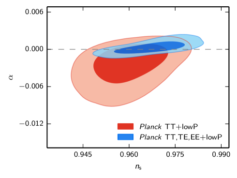
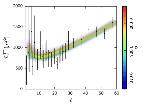
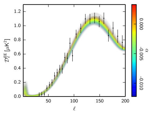
Planck Collaboration XXII (2014) presented constraints on a variety of general isocurvature models using the Planck temperature data, finding consistency with adiabaticity, though with some mild preference for isocurvature models that reduce the power at low multipoles to provide a better match to the Planck temperature spectrum at . For matter isocurvature perturbations, the photons are initially unperturbed but perturbations develop as the Universe becomes more matter dominated. As a result, the phase of the acoustic oscillations differs from adiabatic modes; this is most clearly distinctive with the addition of polarization data (Bucher et al. 2001a)
An extended analysis of isocurvature models is given in Planck Collaboration XX (2016). Here we focus on a simple illustrative case of a totally-correlated matter isocurvature mode. We define an isocurvature amplitude parameter , such that272727Planck Collaboration XX (2016) gives equivalent one-tailed constraints on , where the correlated and anti-correlated cases are considered separately.
| (1) |
where is the primordial curvature perturbation. Here is the total matter isocurvature mode, defined as the observable sum of the baryon and CDM isocurvature modes, i.e., , where
| (2) |
All modes are assumed to have a power spectrum with the same spectral index , so that is independent of scale. For positive this agrees with the definitions in Bean et al. (2006) and Larson et al. (2011) for , but also allows for the correlation to have the opposite sign. Approximately, , where is the CDM version of the amplitude defined as in Amendola et al. (2002). Note that in our conventions, negative values of lower the Sachs–Wolfe contribution to the large-scale power spectrum. We caution the reader that this convention differs from some others, e.g., Larson et al. (2011).
Planck constraints on the correlated isocurvature amplitude are shown in Fig. 24, with and without high-multipole polarization. The corresponding marginalized limit from the temperature data is
| (3) |
which is significantly tightened around zero when Planck polarization information is included at high multipoles:
| (4) |
This strongly limits the isocurvature contribution to be less than about 3 % of the adiabatic modes. Figure 25 shows how models with negative correlation parameter, , fit the temperature data at low multipoles slightly better than models with ; however, these models are disfavoured from the corresponding change in the polarization acoustic peaks.
In this model most of the gain in sensitivity comes from relatively large scales, , where the correlated isocurvature modes with delayed phase change the first polarization acoustic peak () significantly more than in temperature (Bucher et al. 2001a). The polarization data are not entirely robust to systematics on these scales, but in this case the result appears to be quite stable between the different likelihood codes. However, it should be noted that a particularly low point in the spectrum at (see Fig. 3) pulls in the direction of positive , and could be giving an artificially strong constraint if this were caused by an unidentified systematic.
6.2.4 Curvature
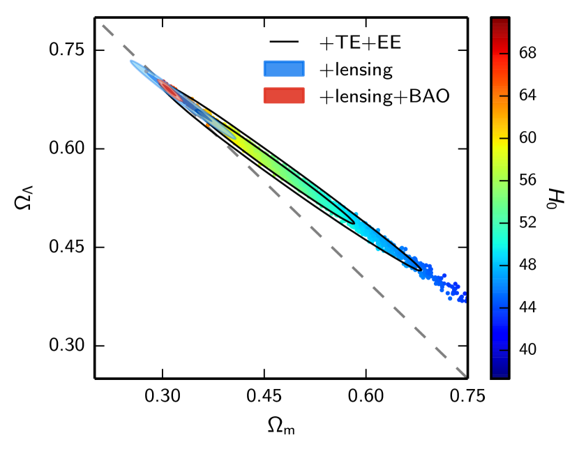
The simplifying assumptions of large-scale homogeneity and isotropy lead to the familiar Friedman-Lemaître-Robertson-Walker (FLRW) metric that appears to be an accurate description of our Universe. The base cosmology assumes an FLRW metric with a flat 3-space. This is a very restrictive assumption that needs to be tested empirically. In this subsection, we investigate constraints on the parameter , where for models . For FLRW models corresponds to negatively-curved 3-geometries while corresponds to positively-curved 3-geometries. Even with perfect data within our past lightcone, our inference of the curvature is limited by the cosmic variance of curvature perturbations that are still super-horizon at the present, since these cannot be distinguished from background curvature within our observable volume.
The parameter decreases exponentially with time during inflation, but grows only as a power law during the radiation and matter-dominated phases, so the standard inflationary prediction has been that curvature should be unobservably small today. Nevertheless, by fine-tuning parameters it is possible to devise inflationary models that generate open (e.g., Bucher et al. 1995; Linde 1999) or closed universes (e.g., Linde 2003). Even more speculatively, there has been interest recently in multiverse models, in which topologically-open “pocket universes” form by bubble nucleation (e.g., Coleman & De Luccia 1980; Gott 1982) between different vacua of a “string landscape” (e.g., Freivogel et al. 2006; Bousso et al. 2015). Clearly, the detection of a significant deviation from would have profound consequences for inflation theory and fundamental physics.
The Planck power spectra give the constraint
| (5) |
The well-known geometric degeneracy (Bond et al. 1997; Zaldarriaga et al. 1997) allows for the small-scale linear CMB spectrum to remain almost unchanged if changes in are compensated by changes in to obtain the same angular diameter distance to last scattering. The Planck constraint is therefore mainly determined by the (wide) priors on , and the effect of lensing smoothing on the power spectra. As discussed in Sect. 5.1, the Planck temperature power spectra show a slight preference for more lensing than expected in the base cosmology, and since positive curvature increases the amplitude of the lensing signal, this preference also drives towards negative values.
Taken at face value, Eq. (5) represents a detection of positive curvature at just over , largely via the impact of lensing on the power spectra. One might wonder whether this is mainly a parameter volume effect, but that is not the case, since the best fit closed model has relative to base , and the fit is improved over almost all the posterior volume, with the mean improvement being (very similar to the phenomenological case of +). Addition of the Planck polarization spectra shifts towards zero by :
| (6) |
but remains negative at just over .
What’s more, the lensing reconstruction from Planck measures the lensing amplitude directly and, as discussed in Sect. 5.1, this does not prefer more lensing than base . The combined constraint shows impressive consistency with a flat universe:
| (7) |
The dramatic improvement in the error bar is another illustration of the power of the lensing reconstruction from Planck.
The constraint can be sharpened further by adding external data that break the main geometric degeneracy. Combining the Planck data with BAO, we find
| (8) |
This constraint is unchanged at the quoted precision if we add the JLA supernovae data and the prior of Eq. (1).
6.3 Dark energy
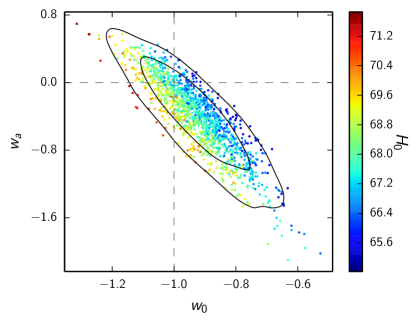
The physical explanation for the observed accelerated expansion of the Universe is currently not known. In standard the acceleration is provided by a cosmological constant, i.e., an additional fluid satisfying an equation of state . However, there are many possible alternatives, typically described either in terms of extra degrees of freedom associated with scalar fields or modifications of general relativity on cosmological scales (for reviews see, e.g., Copeland et al. 2006; Tsujikawa 2010). A detailed study of these models and the constraints imposed by Planck and other data are presented in a separate paper, Planck Collaboration XIV (2016).
Here we will limit ourselves to the most basic extensions of , which can be phenomenologically described in terms of the equation of state parameter alone. Specifically we will use the camb implementation of the “parameterized post-Friedmann” (PPF) framework of Hu & Sawicki (2007) and Fang et al. (2008) to test whether there is any evidence that varies with time. This framework aims to recover the behaviour of canonical (i.e., those with a standard kinetic term) scalar field cosmologies minimally coupled to gravity when , and accurately approximates them for values . In these models the speed of sound is equal to the speed of light, so that the clustering of the dark energy inside the horizon is strongly suppressed. The advantage of using the PPF formalism is that it is possible to study the phantom domain, , including transitions across the “phantom barrier,” , which is not possible for canonical scalar fields.
The CMB temperature data alone do not tightly constrain , because of a strong geometrical degeneracy, even for spatially-flat models. From Planck we find
| (9) |
i.e., almost a shift into the phantom domain. This is partly, but not entirely, a parameter volume effect, with the average effective improving by compared to base . This is consistent with the preference for a higher lensing amplitude discussed in Sect. 5.1.2, improving the fit in the region, where the lensing smoothing amplitude becomes slightly larger. However, the lower limit in Eq. (9) is largely determined by the (arbitrary) prior , chosen for the Hubble parameter. Much of the posterior volume in the phantom region is associated with extreme values for cosmological parameters, which are excluded by other astrophysical data. The mild tension with base disappears as we add more data that break the geometrical degeneracy. Adding Planck lensing and BAO, JLA and (“ext”) gives the 95 % constraints
| (0a) | |||||
| (0b) | |||||
| (0c) | |||||
The addition of Planck lensing, or using the full Planck temperature+polarization likelihood together with the BAO, JLA, and data does not substantially improve the constraint of Eq. (0a). All of these data set combinations are compatible with the base value of . In PCP13, we conservatively quoted , based on combining Planck with BAO, as our most reliable limit on . The errors in Eqs. (0a)–(0c) are substantially smaller, mainly because of the addition of the JLA SNe data, which offer a sensitive probe of the dark energy equation of state at . In PCP13, the addition of the SNLS SNe data pulled into the phantom domain at the level, reflecting the tension between the SNLS sample and the Planck 2013 base parameters. As noted in Sect. 5.3, this discrepancy is no longer present, following improved photometric calibrations of the SNe data in the JLA sample. One consequence of this is the tightening of the errors in Eqs. (0a)–(0c) around the value when we combine the JLA sample with Planck.
If differs from , it is likely to change with time. We consider here the case of a Taylor expansion of at first order in the scale factor, parameterized by
| (1) |
More complex models of dynamical dark energy are discussed in Planck Collaboration XIV (2016). Figure 27 shows the 2D marginalized posterior distribution for and for the combination Planck+BAO+JLA. The JLA SNe data are again crucial in breaking the geometrical degeneracy at low redshift and with these data we find no evidence for a departure from the base cosmology. The points in Fig. 27 show samples from these chains colour-coded by the value of . From these MCMC chains, we find . Much higher values of would favour the phantom regime, .
As pointed out in Sects. 5.5.2 and 5.6 the CFHTLenS weak lensing data are in tension with the Planck base parameters. Examples of this tension can be seen in investigations of dark energy and modified gravity, since some of these models can modify the growth rate of fluctuations from the base predictions. This tension can be seen even in the simple model of Eq. (1). The green regions in Fig. 28 show 68 % and 95 % contours in the – plane for Planck TT+lowP combined with the CFHTLenS H13 data. In this example, we have applied ultra-conservative cuts, excluding entirely and excluding measurements with ′ in for all tomographic redshift bins. As discussed in Planck Collaboration XIV (2016), with these cuts the CFHTLenS data are insensitive to modelling the nonlinear evolution of the power spectrum, but this reduction in sensitivity comes at the expense of reducing the statistical power of the weak lensing data. Nevertheless, Fig. 28 shows that the combination of Planck+CFHTLenS pulls the contours into the phantom domain and is discrepant with base at about the level. The Planck+CFHTLenS data also favour a high value of . If we add the (relatively weak) prior of Eq. (1), the contours (shown in cyan) in Fig. 28 shift towards . It therefore seems unlikely that the tension between Planck and CFHTLenS can be resolved by allowing a time-variable equation of state for dark energy.
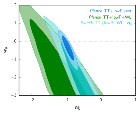
A much more extensive investigation of models of dark energy and also models of modified gravity can be found in Planck Collaboration XIV (2016). The main conclusions of that analysis are as follows:
-
an investigation of more general time-variations of the equation of state shows a high degree of consistency with ;
-
a study of several dark energy and modified gravity models either finds compatibility with base , or mild tensions, which are driven mainly by external data sets.
6.4 Neutrino physics and constraints on relativistic components
In the following subsections, we update Planck constraints on the mass of standard (active) neutrinos, additional relativistic degrees of freedom, models with a combination of the two, and models with massive sterile neutrinos. In each subsection we emphasize the Planck-only constraint, and the implications of the Planck result for late-time cosmological parameters measured from other observations. We then give a brief discussion of tensions between Planck and some discordant external data, and assess whether any of these model extensions can help to resolve them. Finally we provide constraints on neutrino interactions.
6.4.1 Constraints on the total mass of active neutrinos
Detection of neutrino oscillations has proved that neutrinos have mass (see, e.g., Lesgourgues & Pastor 2006 and Nakamura & Petcov 2014 for reviews). The Planck base model assumes a normal mass hierarchy with (dominated by the heaviest neutrino mass eigenstate) but there are other possibilities, including a degenerate hierarchy with . At this time there are no compelling theoretical reasons to strongly prefer any of these possibilities, so allowing for larger neutrino masses is perhaps one of the most well-motivated extensions to base considered in this paper. There has also been significant interest recently in larger neutrino masses as a possible way to lower (the late-time fluctuation amplitude), and thereby reconcile Planck with weak lensing measurements and the abundance of rich clusters (see Sects. 5.5 and 5.6). Though model dependent, neutrino mass constraints from cosmology are already significantly stronger than those from tritium -decay experiments (see, e.g., Drexlin et al. 2013).
Here we give constraints assuming three species of degenerate massive neutrinos, neglecting the small differences in mass expected from the observed mass splittings. At the level of sensitivity of Planck this is an accurate approximation, but note that it does not quite match continuously on to the base model (which assumes two massless and one massive neutrino with ). We assume that the neutrino mass is constant, and that the distribution function is Fermi-Dirac with zero chemical potential.
Masses well below have only a mild effect on the shape of the CMB power spectra, since they became non-relativistic after recombination. The effect on the background cosmology can be compensated by changes in , to ensure the same observed acoustic peak scale . There is, however, some sensitivity of the CMB anisotropies to neutrino masses as the neutrinos start to become less relativistic at recombination (modifying the early ISW effect), and from the late-time effect of lensing on the power spectrum. The Planck power spectrum (95 %) constraints are
| (0a) | |||||
| (0b) | |||||
| (0c) | |||||
| (0d) |
The Planck TT+lowP constraint has a broad tail to high masses, as shown in Fig. 29, which also illustrates the acoustic scale degeneracy with . Larger masses imply a lower through the effects of neutrino free-streaming on structure formation, but the larger masses also require a lower Hubble constant, leading to possible tensions with direct measurements of . Masses below about can provide an acceptable fit to the direct measurements, and adding the BAO data helps to break the acoustic scale degeneracy and tightens the constraint on substantially. Adding Planck polarization data at high multipoles produces a relatively small improvement to the Planck TT+lowP+BAO constraint (and the improvement is even smaller with the alternative CamSpec likelihood), so we consider the results to be our most reliable constraints.
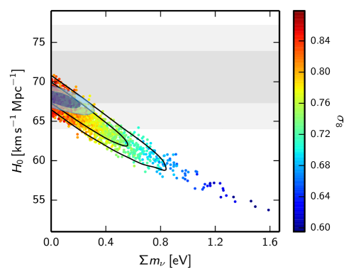
The constraint of Eq. (0b) is consistent with the 95 % limit of reported in PCP13 for Planck+BAO. The limits are similar because the linear CMB is insensitive to the mass of neutrinos that are relativistic at recombination. There is little to be gained from improved measurement of the CMB temperature power spectra, though improved external data can help to break the geometric degeneracy to higher precision. CMB lensing can also provide additional information at lower redshifts, and future high-resolution CMB polarization measurements that accurately reconstruct the lensing potential can probe much smaller masses (see, e.g. Abazajian et al. 2015b).
As discussed in detail in PCP13 and Sect. 5.1, the Planck CMB power spectra prefer somewhat more lensing smoothing than predicted in (allowing the lensing amplitude to vary gives at just over ). The neutrino mass constraint from the power spectra is therefore quite tight, since increasing the neutrino mass lowers the predicted smoothing even further compared to base . On the other hand the lensing reconstruction data, which directly probes the lensing power, prefers lensing amplitudes slightly below (but consistent with) the base prediction (Eq. 1). The Planck+lensing constraint therefore pulls the constraints slightly away from zero towards higher neutrino masses, as shown in Fig. 30. Although the posterior has less weight at zero, the lensing data are incompatible with very large neutrino masses so the Planck+lensing 95 % limit is actually tighter than the Planck TT+lowP result:
| (1) |
Adding the polarization spectra improves this constraint slightly to
| (2) |
We take the combined constraint that further includes BAO, JLA, and (“ext”) as our best limit:
| (3) |
This is slightly weaker than the constraint from Planck TT,TE,EE+lowP+lensing+BAO (which is tighter in both the CamSpec and Plik likelihoods), but is immune to low level systematics that might affect the constraints from the Planck polarization spectra. Equation (3) is therefore a conservative limit. Marginalizing over the range of neutrino masses, the Planck constraints on the late-time parameters are282828To simplify the displayed equations, is given in units of in this section.
| (4) |
For this restricted range of neutrino masses, the impact on the other cosmological parameters is small and, in particular, low values of will remain in tension with the parameter space preferred by Planck.
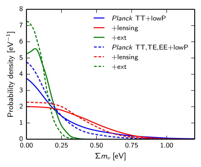
The constraint of Eq. (3) is weaker than the constraint of Eq. (0b) excluding lensing, but there is no good reason to disregard the Planck lensing information while retaining other astrophysical data. The CMB lensing signal probes very-nearly linear scales and passes many consistency checks over the multipole range used in the Planck lensing likelihood (see Sect. 5.1 and Planck Collaboration XV 2016). The situation with galaxy weak lensing is rather different, as discussed in Sect. 5.5.2. In addition to possible observational systematics, the weak lensing data probe lower redshifts than CMB lensing, and smaller spatial scales, where uncertainties in modelling nonlinearities in the matter power spectrum and baryonic feedback become important (Harnois-Déraps et al. 2015).
A larger range of neutrino masses was found by Beutler et al. (2014) using a combination of RSD, BAO, and weak lensing information. The tension between the RSD results and base was subsequently reduced following the analysis of Samushia et al. (2014), as shown in Fig. 17. Galaxy weak lensing and some cluster constraints remain in tension with base , and we discuss possible neutrino resolutions of these problems in Sect. 6.4.4.
Another way of potentially improving neutrino mass constraints is to use measurements of the Ly flux power spectrum of high-redshift quasars. Palanque-Delabrouille et al. (2015) have recently reported an analysis of a large sample of quasar spectra from the SDSSIII/BOSS survey. When combining their results with 2013 Planck data, these authors find a bound (95 % CL), compatible with the results presented in this section.
An exciting future prospect is the possible direct detection of non-relativistic cosmic neutrinos by capture on tritium, for example with the PTOLEMY experiment (Cocco et al. 2007; Betts et al. 2013; Long et al. 2014). Unfortunately, for the mass range preferred by Planck, detection with the first generation experiment will be extremely difficult.
6.4.2 Constraints on
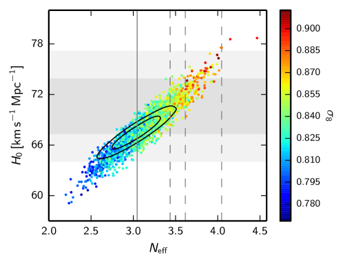
Dark radiation density in the early Universe is usually parameterized by , defined so that the total relativistic energy density in neutrinos and any other dark radiation is given in terms of the photon density at by
| (5) |
The numerical factors in this equation are included so that for three standard model neutrinos that were thermalized in the early Universe and decoupled well before electron-positron annihilation. The standard cosmological prediction is actually , since neutrinos are not completely decoupled at electron-positron annihilation and are subsequently slightly heated (Mangano et al. 2002).
In this section we focus on additional energy density from massless particles. In addition to massless sterile neutrinos, a variety of other particles could contribute to . We assume that the additional massless particles are produced well before recombination, and neither interact nor decay, so that their energy density scales with the expansion exactly like massless neutrinos. An additional could correspond to a fully thermalized sterile neutrino that decoupled at ; for example, any sterile neutrino with mixing angles large enough to provide a potential resolution to short-baseline reactor neutrino oscillation anomalies would most likely thermalize rapidly in the early Universe. However, this solution to the neutrino oscillation anomalies requires approximately 1-eV sterile neutrinos, rather than the massless case considered in this section; exploration of the two parameters and is reported in Sect. 6.4.3. For a review of sterile neutrinos see Abazajian et al. (2012).
More generally the additional radiation does not need to be fully thermalized, for example there are many possible models of non-thermal radiation production via particle decays (see, e.g., Hasenkamp & Kersten 2013; Conlon & Marsh 2013). The radiation could also be produced at temperatures , in which case typically for each additional species, since heating by photon production at muon annihilation (corresponding to ) decreases the fractional importance of the additional component at the later times relevant for the CMB. For particles produced at the density would be diluted even more by numerous phase transitions and particle annihilations, and give . Furthermore, if the particle is not fermionic, the factors entering the entropy conservation equation are different, and even thermalized particles could give specific fractional values of . For example Weinberg (2013) considers the case of a thermalized massless boson, which contributes if it decouples in the range like the neutrinos, or if it decouples at (before the photon production at muon annihilation, hence undergoing fractional dilution).
In this paper we follow the usual phenomenological approach, where one constrains as a free parameter with a wide flat prior, although we comment on a few discrete cases separately below. Values of are less well motivated, since they would require the standard neutrinos to be incompletely thermalized or additional photon production after neutrino decoupling, but we include this range for completeness.
Figure 31 shows that Planck is entirely consistent with the standard value . However, a significant density of additional radiation is still allowed, with the (68 %) constraints
| (0a) | |||||
| (0b) | |||||
| (0c) | |||||
| (0d) |
Notice the significantly tighter constraint with the inclusion of Planck high- polarization, with at over from Planck alone. This constraint is not very stable between likelihoods, with the CamSpec likelihood giving a roughly lower value of . However, the strong limit from polarization is also consistent with the joint Planck TT+lowP+BAO result, so Eq. (0b) leads to the robust conclusion that at over . The addition of Planck lensing has very little effect on this constraint.
For , the Planck data favour higher values of the Hubble parameter than the Planck base value, which as discussed in Sect. 5.4 may be in better agreement with some direct measurements of . This is because Planck accurately measures the acoustic scale ; increasing means (via the Friedmann equation) that the early Universe expands faster, so the sound horizon at recombination, , is smaller and hence recombination has to be closer (larger and hence smaller ) for it to subtend the same angular size observed by Planck. However, models with and a higher Hubble constant also have higher values of the fluctuation amplitude , as shown by the coloured samples in Fig. 31. As a result, these models increase the tensions between the CMB measurements and astrophysical measurements of discussed in Sect. 5.6. It therefore seems unlikely that additional radiation alone can help to resolve tensions with large-scale structure data.
The energy density in the early Universe can also be probed by the predictions of BBN. In particular increases the primordial expansion rate, leading to earlier freeze-out, with a higher neutron density and hence a greater abundance of helium and deuterium after BBN has completed. A detailed discussion of the implications of Planck for BBN is given in Sect. 6.5. Observations of both the primordial helium and deuterium abundance are compatible with the predictions of standard BBN for the Planck base value of the baryon density. The Planck+BBN constraints on (Eqs. 7 and 8) are compatible, and slightly tighter than Eq. (0b).
Although there is a large continuous range of plausible values, it is worth mentioning briefly a few of the discrete values from fully thermalized models. This serves as an indication of how strongly Planck prefers base , and also how the inferred values of other cosmological parameters might be affected by this particular extension to base . As discussed above, one fully thermalized neutrino () is ruled out at over , and is disfavoured by compared to base by Planck TT+lowP, and much more strongly in combination with Planck high- polarization or BAO data. The thermalized boson models that give or are disfavoured by and , respectively, and are therefore not strongly excluded. We focus on the former, since it is also consistent with the Planck TT+lowP+BAO constraint at . As shown in Fig. 31, larger corresponds to a region of parameter space with significantly higher Hubble parameter,
| (1) |
This can be compared to the direct measurements of discussed in Sect. 5.4. Evidently, Eq. (1) is consistent with the prior adopted in this paper (Eq. 1), but this example shows that an accurate direct measurement of can potentially provide evidence for new physics beyond that probed by Planck. As shown in Fig. 31, the cosmology also has a significantly higher small-scale fluctuation amplitude and the spectral index is also bluer, with
| (2) |
The range in this model is higher than preferred by the Planck lensing likelihood in base . However, the fit to the Planck lensing likelihood is model dependent and the lensing degeneracy direction also associates high and low values with higher . The joint Planck TT+lowP+lensing constraint does pull down slightly to and provides an acceptable fit to the Planck data. For Planck TT+lowP+lensing, the difference in between the best fit base model and the extension with is only . The higher spectral index with gives a decrease in large-scale power, fitting the low Planck spectrum better by , but at the same time the high- data prefer . Correlations with other cosmological parameters can be seen in Fig. 20. Clearly, a very effective way of testing these models would be to obtain reliable, accurate, astrophysical measurements of and .
In summary, models with are disfavoured by Planck combined with BAO data at about the level. Models with fractional changes of are mildly disfavoured by Planck, but require higher and compared to base .
6.4.3 Simultaneous constraints on and neutrino mass
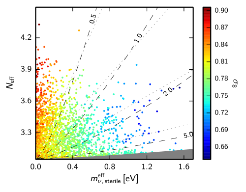
As discussed in the previous sections, neither a higher neutrino mass nor additional radiation density alone can resolve all of the tensions between Planck and other astrophysical data. However, the presence of additional massive particles, such as massive sterile neutrinos, could potentially improve the situation by introducing enough freedom to allow higher values of the Hubble constant and lower values of . As mentioned in Sect. 6.4.2, massive sterile neutrinos offer a possible solution to reactor neutrino oscillation anomalies (Kopp et al. 2013; Giunti et al. 2013) and this has led to significant recent interest in this class of models (Hamann & Hasenkamp 2013; Wyman et al. 2014; Battye & Moss 2014; Leistedt et al. 2014; Bergström et al. 2014; MacCrann et al. 2015). Alternatively, active neutrinos could have significant degenerate masses above the minimal baseline value together with additional massless particles contributing to . Many more complicated scenarios could also be envisaged.
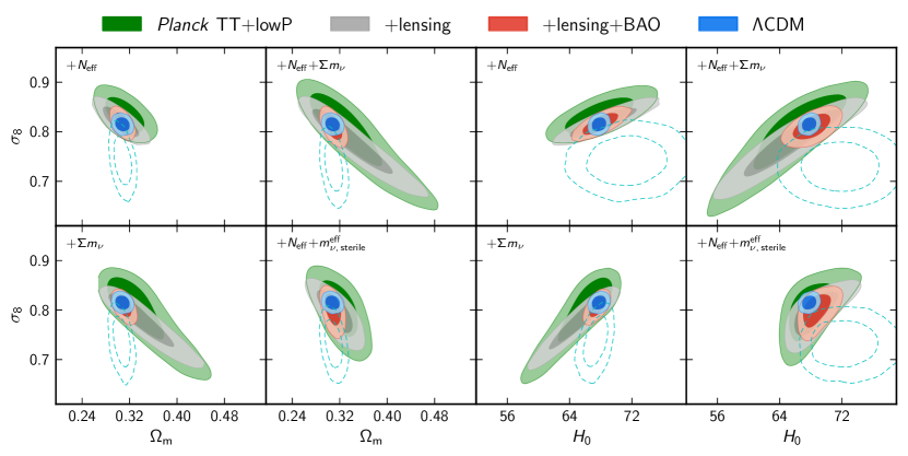
In the case of massless radiation density, the cosmological predictions are independent of the actual form of the distribution function, since all particles travel at the speed of light. However, for massive particles the results are more model dependent. To formulate a well-defined model, we follow PCP13 and consider the case of one massive sterile neutrino parameterized by , in addition to the two approximately massless and one massive neutrino of the baseline model. For thermally-distributed sterile neutrinos, is related to the true mass via
| (3) |
and for the cosmologically-equivalent Dodelson-Widrow (DW) case (Dodelson & Widrow 1994) the relation is given by
| (4) |
with . We impose a prior on the physical thermal mass, , when generating parameter chains, to exclude regions of parameter space in which the particles are so massive that their effect on the CMB spectra is identical to that of cold dark matter. Although we consider only the specific case of one massive sterile neutrino with a thermal (or DW) distribution, our constraints will be reasonably accurate for other models, for example eV-mass particles produced as non-thermal decay products (Hasenkamp 2014).
Figure 32 shows that although Planck is perfectly consistent with no massive sterile neutrinos, a significant region of parameter space with fractional is allowed, where is lower than in the base model. This is also the case for massless sterile neutrinos combined with massive active neutrinos. In the single massive sterile model, the combined constraints are
| (5) |
The upper tail of is largely associated with high physical masses near to the prior cutoff; if instead we restrict to the region where the constraint is
| (6) |
Massive sterile neutrinos with mixing angles large enough to help resolve the reactor anomalies would typically imply full thermalization in the early Universe, and hence give for each additional species. Such a high value of , especially combined with , as required by reactor anomaly solutions, were virtually ruled out by previous cosmological data (Mirizzi et al. 2013; Archidiacono et al. 2013a; Gariazzo et al. 2013). This conclusion is strengthened by the analysis presented here, since is excluded at greater than 99 % confidence. Unfortunately, there does not appear to be a consistent resolution to the reactor anomalies, unless thermalization of the massive neutrinos can be suppressed, for example, by large lepton asymmetry, new interactions, or particle decay (see Gariazzo et al. 2014; Bergström et al. 2014, and references therein).
We have also considered the case of additional radiation and degenerate massive active neutrinos, with the combined constraint
| (7) |
Again Planck shows no evidence for a deviation from the base model.
6.4.4 Neutrino models and tension with external data
The extended models discussed in this section allow Planck to be consistent with a wider range of late-Universe parameters than in base . Figure 33 summarizes the constraints on , , and for the various models that we have considered. The inferred Hubble parameter can increase or decrease, as required to maintain the observed acoustic scale, depending on the relative contribution of additional radiation (changing the sound horizon) and neutrino mass (changing mainly the angular diameter distance). However, all of the models follow similar degeneracy directions in the – and – planes, so these models remain predictive: large common areas of the parameter space are excluded in all of these models. The two-parameter extensions are required to fit substantially lower values of without also decreasing below the values determined from direct measurements, but the scope for doing this is clearly limited.
External data sets need to be reanalysed consistently in extended models, since the extensions change the growth of structure, angular distances, and the matter-radiation equality scale. For example, the dashed lines in Fig. 33 show how different models affect the CFHTLenS galaxy weak lensing constraints from Heymans et al. (2013) (see Sect. 5.5.2), when restricted to the region of parameter space consistent with the Planck acoustic scale measurements and the local Hubble parameter. The filled green, grey, and red contours in Fig. 33 show the CMB constraints on these models for various data combinations. The tightest of these constraints comes from the Planck TT+lowP+lensing+BAO combination. The blue contours show the constraints in the base cosmology. The red contours are broader than the blue contours and there is greater overlap with the CFHTLenS contours, but this offers only a marginal improvement compared to base (compare with Fig. 18; see also the discussions in Leistedt et al. 2014 and Battye et al. 2015). For each of these models, the CFHTLenS results prefer lower values of . Allowing for a higher neutrino mass lowers from Planck, but does not help alleviate the discrepancy with the CFHTLenS data, since the Planck data prefer a lower value of . A joint analysis of the CFHTLenS likelihood with Planck TT+lowP shows a preference for the extended neutrino models compared to base , and the fits to Planck TT+lowP are worse in all cases. In base the CFHTLenS data prefer a region of parameter space away from the Planck TT+lowP+CFHTLenS joint fit, indicative of the tension between the data sets. This is only slightly relieved to in the extended models.
In summary, modifications to the neutrino sector alone cannot easily explain the discrepancies between Planck and other astrophysical data described in Sect. 5.5, including the inference of a low value of from rich cluster counts.
6.4.5 Testing perturbations in the neutrino background
As shown in the previous sections, the Planck data provide evidence for a cosmic neutrino background at a very high significance level. Neutrinos affect the CMB anisotropies at the background level, by changing the expansion rate before recombination and hence relevant quantities such as the sound horizon and the damping scales. Neutrinos also affect the CMB anisotropies via their perturbations. Perturbations in the neutrino background are coupled through gravity to the perturbations in the photon background, and can be described (for massless neutrinos) by the following set of equations (Hu 1998; Hu et al. 1999; Trotta & Melchiorri 2005; Archidiacono et al. 2011):
| (0a) | |||||
| (0b) | |||||
| (0c) | |||||
| (0d) |
Here dots denote derivatives with respect to conformal time, is the neutrino density contrast, is the neutrino velocity perturbation, the anisotropic stress, are higher-order moments of the neutrino distribution function, and and are the scalar metric perturbations in the synchronous gauge. In these equations, is the neutrino sound speed in its own reference frame and parameterizes the anisotropic stress. For standard non-interacting massless neutrinos . Any deviation from the expected values could provide a hint of non-standard physics in the neutrino sector.
A greater (lower) neutrino sound speed would increase (decrease) the neutrino pressure, leading to a lower (higher) perturbation amplitude. On the other hand, changing alters the viscosity of the neutrino fluid. For , the neutrinos act as a perfect fluid, supporting undamped acoustic oscillations.
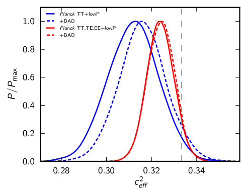
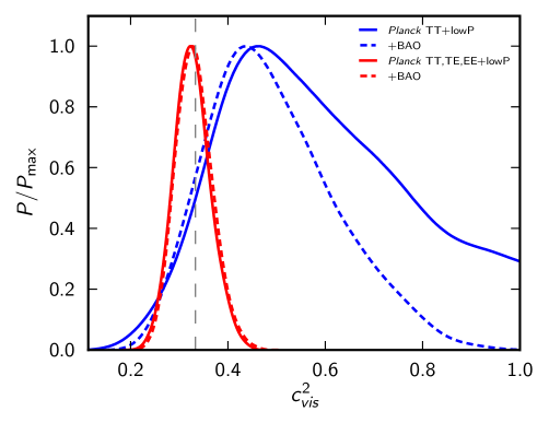
Several previous studies have used this approach to constrain and using cosmological data (see, e.g., Trotta & Melchiorri 2005; Smith et al. 2012; Archidiacono et al. 2013b; Gerbino et al. 2013; Audren et al. 2015), with the motivation that deviations from the expected values could be a hint of non-standard physics in the neutrino sector. Non-standard interactions could involve, for example, neutrino coupling with light scalar particles (Hannestad 2005; Beacom et al. 2004; Bell 2005; Sawyer 2006). If neutrinos are strongly coupled at recombination, this would result in a lower value for than in the standard model. Alternatively, the presence of early dark energy that mimics a relativistic component at recombination could possibly lead to a value for that differs from (see, e.g., Calabrese et al. 2011).
In this analysis, for simplicity, we assume and massless neutrinos. By using an equivalent parameterization for massive neutrinos (Audren et al. 2015) we have checked that assuming one massive neutrino with eV, as in the base model used throughout this paper, has no impact on the constraints on and reported in this section.292929We also do not explore extended cosmologies in this section, since no significant degeneracies are expected between (, , , ) and (, ) (Audren et al. 2015). We adopt a flat prior between zero and unity for both and .
The top and bottom panels of Fig. 34 show the posterior distributions of and from Planck TT+lowP, Planck TT+lowP+BAO, Planck TT,TE,EE+lowP, and Planck TT,TE,EE+lowP+BAO. The mean values and 68 % errors on and are
| (1a) | |||
| (1b) | |||
| (1c) | |||
| (1d) |
Constraints on these parameters are consistent with the conventional values . A vanishing value of , which might imply a strong interaction between neutrinos and other species, is excluded at more than the level arising from the Planck temperature data. This conclusion is greatly strengthened (to about ) when Planck polarization data are included. As discussed in Bashinsky & Seljak (2004), neutrino anisotropic stresses introduce a phase shift in the CMB angular power spectra, which is more visible in polarization than temperature because of the sharper acoustic peaks. This explains why we see such a dramatic reduction in the error on when including polarization data.
The precision of our results is consistent with the forecasts discussed in Smith et al. (2012), and we find strong evidence, purely from CMB observations, for neutrino anisotropies with the standard values and .
6.5 Primordial nucleosynthesis
6.5.1 Details of analysis approach
Standard big bang nucleosynthesis (BBN) predicts light element abundances as a function of parameters relevant to the CMB, such as the baryon-to-photon density ratio , the radiation density parameterized by , and the chemical potential of the electron neutrinos. In PCP13, we presented consistency checks between the Planck 2013 results, light element abundance data, and standard BBN. The goal of Sect. 6.5.2 below is to update these results and to provide improved tests of the standard BBN model. In Sect. 6.5.3 we show how Planck data can be used to constrain nuclear reaction rates, and in Sect. 6.5.4 we will present the most stringent CMB bounds to date on the primordial helium fraction.
For simplicity, our analysis assumes a negligible leptonic asymmetry in the electron neutrino sector. For a fixed photon temperature today (which we take to be K), can be related to , up to a small (and negligible) uncertainty associated with the primordial helium fraction. Standard BBN then predicts the abundance of each light element as a function of only two parameters, and , with a theoretical error coming mainly from uncertainties in the neutron lifetime and a few nuclear reaction rates.
We will confine our discussion to BBN predictions for the primordial abundances303030BBN calculations usually refer to nucleon number density fractions rather than mass fractions. To avoid any ambiguity with the helium mass fraction , normally used in CMB physics, we use superscripts to distinguish between the two definitions and . Typically, is about 0.5 % higher than . of 4He and deuterium, expressed, respectively as and . We will not discuss other light elements, such as tritium and lithium, because the observed abundance measurements and their interpretation is more controversial (see Fields et al. 2014, for a recent review). As in PCP13, the BBN predictions for ) and ) are given by Taylor expansions obtained with the PArthENoPE code (Pisanti et al. 2008), similar to the ones presented in Iocco et al. (2009), but updated by the PArthENoPE team with the latest observational data on nuclear rates and on the neutron life-time:
| (2) | ||||
| (3) | ||||
By averaging over several measurements, the Particle Data Group 2014 (Olive et al. 2014) estimates the neutron life-time to be at 68 % CL.313131However, the most recent individual measurement by Yue et al. (2013) gives , which is discrepant at with the previous average (including only statistical errors). Hence one should bear in mind that systematic effects could be underestimated in the Particle Data Group result. Adopting the central value of Yue et al. (2013) would shift our results by a small amount (by a factor of 1.0062 for and 1.0036 for ). The expansions in Eqs. (2) and (3) are based on this central value, and we assume that Eq. (2) predicts the correct helium fraction up to a standard error , obtained by propagating the error on .
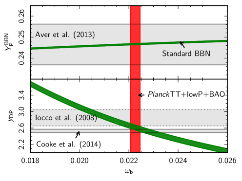
The uncertainty on the deuterium fraction is dominated by that on the rate of the reaction . For that rate, in PCP13 we relied on the result of Serpico et al. (2004), obtained by fitting several experiments. The expansions of Eqs. (2) and (3) now adopt the latest experimental determination by Adelberger et al. (2011) and use the best-fit expression in their equation (29). We also rely on the uncertainty quoted in Adelberger et al. (2011) and propagate it to the deuterium fraction. This gives a standard error , which is more conservative than the error adopted in PCP13.
6.5.2 Primordial abundances from Planck data and standard BBN
We first investigate the consistency of standard BBN and the CMB by fixing the radiation density to its standard value, i.e., , based on the assumption of standard neutrino decoupling and no extra light relics. We can then use Planck data to measure , assuming base , and test for consistency with experimental abundance measurements. The 95 % CL bounds obtained for the base CDM model for various data combinations are
| (4) |
corresponding to a predicted primordial 4He number density fraction (95 % CL) of
| (5) |
and deuterium fraction (95 % CL)
| (6) |
The first set of error bars (in parentheses) in Eqs. (5) and (6) reflect only the uncertainty on . The second set includes the theoretical uncertainty on the BBN predictions, added in quadrature to the errors from . The total errors in the predicted helium abundances are dominated by the BBN uncertainty, as in PCP13. For deuterium, the Planck 2015 results improve the determination of to the point where the theoretical errors are comparable or larger than the errors from the CMB. In other words, for base the predicted abundances cannot be improved substantially by further measurements of the CMB. This also means that Planck results can, in principle, be used to investigate nuclear reaction rates that dominate the theoretical uncertainty (see Sect. 6.5.3).
The results of Eqs. (5) and (6) are well within the ranges indicated by the latest measurements of primordial abundances, as illustrated in Fig. 35. The helium data compilation of Aver et al. (2013) gives (68 % CL), and the Planck prediction is near the middle of this range.323232A substantial part of this error comes from the regression to zero metallicity. The mean of the 17 measurements analysed by Aver et al. (2013) is , i.e., about higher than the Planck predictions of Eq. (5). As summarized by Aver et al. (2013) and Peimbert (2008), helium abundance measurements derived from emission lines in low-metallicity H ii regions are notoriously difficult and prone to systematic errors. As a result, many discrepant helium abundance measurements can be found in the literature. Izotov et al. (2014) have reported , which is discrepant with the base predictions by . Such a high helium fraction could be accommodated by increasing (see Fig. 36 and Sect. 6.5.4); however, at present it is not clear whether the error quoted by Izotov et al. (2014) accurately reflects systematic uncertainties, including in particular the error in extrapolating to zero metallicity.
Historically, deuterium abundance measurements have shown excess scatter over that expected from statistical errors, indicating the presence of systematic uncertainties in the observations. Figure 35 shows the data compilation of Iocco et al. (2009), (68 % CL), which includes measurements based on damped Ly and Lyman limit systems. We also show the more recent results by Cooke et al. (2014) (see also Pettini & Cooke 2012) based on their observations of low-metallicity damped Ly absorption systems in two quasars (SDSS J1358+6522, and SDSS J1419+0829, ) and a reanalysis of archival spectra of damped Ly systems in three further quasars that satisfy strict selection criteria. The Cooke et al. (2014) analysis gives (68 % CL), somewhat lower than the central Iocco et al. (2009) value, and with a much smaller error. The Cooke et al. (2014) value is almost certainly the more reliable measurement, as evidenced by the consistency of the deuterium abundances of the five systems in their analysis. The Planck base predictions of Eq. (6) lie within 1 of the Cooke et al. (2014) result. This is a remarkable success for the standard theory of BBN.
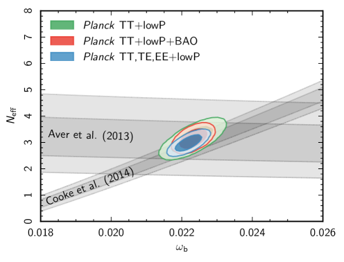
It is worth noting that the Planck data are so accurate that is insensitive to the underlying cosmological model. In our grid of extensions to base the largest degradation of the error in is in models that allow to vary. In these models, the mean value of is almost identical to that for base , but the error on increases by about 30 %. The value of is stable to even more radical changes to the cosmology, for example, adding general isocurvature modes (Planck Collaboration XX 2016).
If we relax the assumption that (but adhere to the hypothesis that electron neutrinos have a standard distribution, with a negligible chemical potential), BBN predictions depend on both parameters and . Following the same methodology as in Sect. 6.4.4 of PCP13, we can identify the region of the – parameter space that is compatible with direct measurements of the primordial helium and deuterium abundances, including the BBN theoretical errors. This is illustrated in Fig. 36 for the extension to base . The region preferred by CMB observations lies at the intersection between the helium and deuterium abundance 68 % CL preferred regions and is compatible with the standard value of . This confirms the beautiful agreement between CMB and BBN physics. Figure 36 also shows that the Planck polarization data help in reducing the degeneracy between and .
We can actually make a more precise statement by combining the posterior distribution on and obtained for Planck with that inferred from helium and deuterium abundance, including observational and theoretical errors. This provides joint CMB+BBN predictions on these parameters. After marginalizing over , the 95 % CL preferred ranges for are
| (7) |
when combining Planck with the helium abundance estimated by Aver et al. (2013), or
| (8) |
when combining with the deuterium abundance measured by Cooke et al. (2014). These bounds represent the best currently-available estimates of and are remarkably consistent with the standard model prediction.
The allowed region in – space does not increase significantly when other parameters are allowed to vary at the same time. From our grid of extended models, we have checked that this conclusion holds in models with neutrino masses, tensor fluctuations, or running of the scalar spectral index, for example.
6.5.3 Constraints from Planck and deuterium observations on nuclear reaction rates
We have seen that primordial element abundances estimated from direct observations are consistent with those inferred from Planck data under the assumption of standard BBN. However, the Planck determination of is so precise that the theoretical errors in the BBN predictions are now a dominant source of uncertainty. As noted by Cooke et al. (2014), one can begin to think about using CMB measurements together with accurate deuterium abundance measurements to learn about the underlying BBN physics.
While for helium the theoretical error comes mainly from the uncertainties in the neutron lifetime, for deuterium it is dominated by uncertainties in the radiative capture process , converting deuterium into helium. The present experimental uncertainty for the -factor at low energy (relevant for BBN), is in the range 6–10 % (Ma et al. 1997). However, as noted by several authors (see, e.g., Nollett & Holder 2011; Di Valentino et al. 2014) the best-fit value of inferred from experimental data in the range is about 5–10 % lower than theoretical expectations (Viviani et al. 2000; Marcucci et al. 2005). The PArthENoPE BBN code assumes the lower experimental value for , and this might explain why the deuterium abundance determined by Cooke et al. (2014) is slightly lower than the value inferred by Planck.
To investigate this further, following the methodology of Di Valentino et al. (2014), we perform a combined analysis of Planck and deuterium observations, to constrain the value of the reaction rate. As in Di Valentino et al. (2014), we parameterize the thermal rate of the process in the PArthENoPE code by introducing a rescaling factor of the experimental rate , i.e., , and solve for using various Planck+BAO data combinations, given the Cooke et al. (2014) deuterium abundance measurements.
Assuming the base model we find (68 % CL)
| (0a) | |||||
| (0b) | |||||
| (0c) | |||||
| (0d) |
The posteriors for are shown in Fig. 37. These results suggest that the reaction rate may be have been underestimated by about 10 %. Evidently, tests of the standard BBN picture appear to have reached the point where they are limited by uncertainties in nuclear reaction rates. There is therefore a strong case to improve the precision of experimental measurements (e.g., Anders et al. 2014) and theoretical computations of key nuclear reaction rates relevant for BBN.
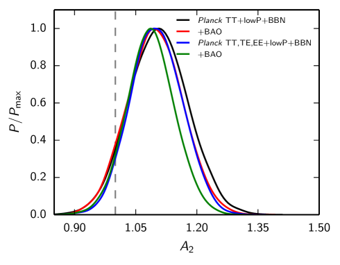
6.5.4 Model-independent bounds on the helium fraction from Planck
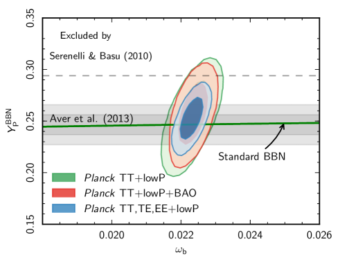
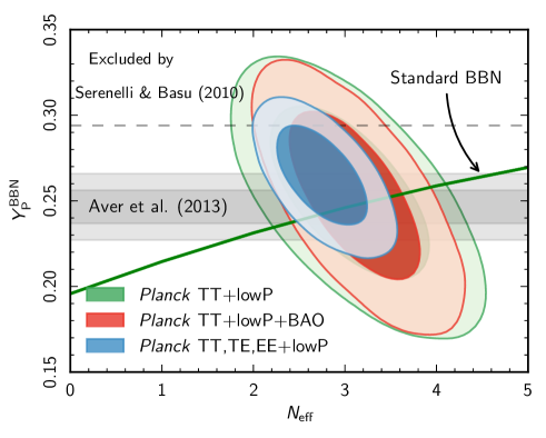
Instead of inferring the primordial helium abundance from BBN codes using constraints from Planck, we can measure it directly, since variations in modify the density of free electrons between helium and hydrogen recombination and therefore affect the damping tail of the CMB anisotropies.
If we allow to vary as an additional parameter to base , we find the following constraints (at 95 % CL):
| (1) |
Joint constraints on and are shown in Fig. 38. The addition of Planck polarization measurements results in a substantial reduction in the uncertainty on the helium fraction. In fact, the standard deviation on in the case of Planck TT,TE,EE+lowP is only 30 % larger than the observational error quoted by Aver et al. (2013). As emphasized throughout this paper, the systematic effects in the Planck polarization spectra, although at low levels, have not been accurately characterized at this time. Readers should therefore treat the polarization constraints with some caution. Nevertheless, as shown in Fig. 38, all three data combinations agree well with the observed helium abundance measurements and with the predictions of standard BBN.
There is a well-known parameter degeneracy between and the radiation density (see the discussion in PCP13). Helium abundance predictions from the CMB are therefore particularly sensitive to the addition of the parameter to base . Allowing both and to vary we find the following constraints (at 95 % CL):
| (2) |
Contours in the – plane are shown in Fig. 39. Here again, the impact of Planck polarization data is important, and helps to substantially reduce the degeneracy between these two parameters. The Planck TT,TE,EE+lowP contours are in very good agreement with standard BBN and . However, even if we relax the assumption of standard BBN, the CMB does not allow high values of . It is therefore difficult to accommodate an extra thermalized relativistic species, even if the standard BBN prior on the helium fraction is relaxed.
6.6 Dark matter annihilation
Energy injection from dark matter (DM) annihilation can alter the recombination history, leading to changes in the temperature and polarization power spectra of the CMB (e.g., Chen & Kamionkowski 2004; Padmanabhan & Finkbeiner 2005). As demonstrated in several papers (e.g., Galli et al. 2009; Slatyer et al. 2009; Finkbeiner et al. 2012), CMB anisotropies offer an opportunity to constrain the nature of DM. Furthermore, CMB experiments such as Planck can achieve limits on the annihilation cross-section that are relevant for the interpretation of the rise in the cosmic-ray positron fraction at energies observed by PAMELA, Fermi, and AMS (Adriani et al. 2009; Ackermann et al. 2012; Aguilar et al. 2014). The CMB constraints are complementary to those determined from other astrophysical probes, such as the -ray observations of dwarf galaxies by the Fermi satellite (Ackermann et al. 2014).
The way in which DM annihilations heat and ionize the gaseous background depends on the nature of the cascade of particles produced following annihilation and, in particular, on the production of pairs and photons that couple to the gas. The fraction of the rest mass energy that is injected into the gas can be modelled by an “efficiency factor,” , which is typically in the range 0.01–1 and depends on redshift.333333To maintain consistency with other papers on dark matter annihilation, we retain the notation for the efficiency factor in this section; it should not be confused with the growth rate factor introduced in Eq. (3). Computations of for various annihilation channels can be found in Slatyer et al. (2009), Hütsi et al. (2009), and Evoli et al. (2013). The rate of energy release per unit volume by annihilating DM can therefore be written as
| (3) |
where is defined as
| (4) |
Here the critical density of the Universe today, is the mass of the DM particle, and is the thermally-averaged annihilation cross-section times the velocity (explicitly the so-called Mller velocity); we will refer to this quantity loosely as the “cross-section” hereafter. In Eq. (3), is a degeneracy factor that is equal to for Majorana particles and for Dirac particles. In this paper, the constraints will refer to Majorana particles. Note that to produce the observed dark matter density from thermal DM relics requires an annihilation cross-section of (assuming s-wave annihilation) at the time of freeze-out (see, e.g., the review by Profumo 2013).
Both the amplitude and redshift dependence of the efficiency factor depend on the details of the annihilation process (e.g., Slatyer et al. 2009). The functional shape of can be taken into account using generalized parameterizations or principal components (Finkbeiner et al. 2012; Hutsi et al. 2011), similar to the analysis of the recombination history presented in Sect. 6.7.4. However, as shown in Galli et al. (2011), Giesen et al. (2012), and Finkbeiner et al. (2012), to a first approximation the redshift dependence of can be ignored, since current CMB data (including Planck) are sensitive to energy injection over a relatively narrow range of redshift, typically –600. The effects of DM annihilation can therefore be reasonably well parameterized by a single constant parameter, (with set to a constant ), which encodes the dependence on the properties of the DM particles. In the following, we calculate constraints on the parameter, assuming that it is constant, and then project these constraints on to a particular dark matter model assuming , since the effect of dark matter annihilation peaks at (see Finkbeiner et al. 2012). The functions used here are those calculated in Slatyer et al. (2009), with the updates described in Galli et al. (2013) and Madhavacheril et al. (2014). Finally, we estimate the fractions of injected energy that affect the gaseous background, from heating, ionizations, or Ly excitations, using the updated calculations described in Galli et al. (2013) and Valdes et al. (2010), following Shull & van Steenberg (1985).
We compute the theoretical angular power spectrum in the presence of DM annihilations by modifying the recfast routine (Seager et al. 1999) in the camb code as in Galli et al. (2011).343434We checked that we obtain similar results using either the HyRec code (Ali-Haimoud & Hirata 2011), as detailed in Giesen et al. (2012), or CosmoRec (Chluba & Thomas 2011), instead of recfast. We then add as an additional parameter to those of the base cosmology. Table 6 shows the constraints for various data combinations.
|
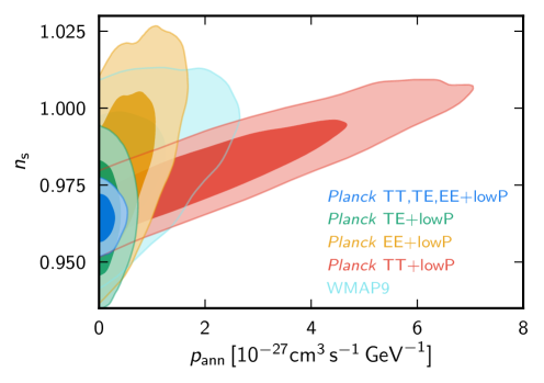
The constraints on from the Planck TT+lowP spectra are about 3 times weaker than the 95 % limit of derived from WMAP9, which includes WMAP polarization data at low multipoles. On the other hand, the Planck or spectra improve the constraints on by about an order of magnitude compared to those from Planck alone. This is because the main effect of dark matter annihilation is to increase the width of last scattering, leading to a suppression of the amplitude of the peaks, both in temperature and polarization. As a result, the effects of DM annihilation on the power spectra at high multipole are degenerate with other parameters of base , such as and (Chen & Kamionkowski 2004; Padmanabhan & Finkbeiner 2005). At large angular scales (), however, dark matter annihilation can produce an enhancement in polarization, caused by the increased ionization fraction in the freeze-out tail following recombination. As a result, large-angle polarization information is crucial for breaking the degeneracies between parameters, as illustrated in Fig. 40. The strongest constraints on therefore come from the full Planck temperature and polarization likelihood and there is little improvement if other astrophysical data, or Planck lensing, are added.353535It is interesting to note that the constraint derived from Planck TT,TE,EE+lowP is consistent with the forecast given in Galli et al. (2009), .
We verified the robustness of the Planck TT,TE,EE+lowP constraint by also allowing other parameter extensions of base CDM (, , or ) to vary together with . We found that the constraint is weakened by up to 20 %. Furthermore, we have verified that we obtain consistent results when relaxing the priors on the amplitudes of the Galactic dust templates or if we use the CamSpec likelihood instead of the baseline Plik likelihood.
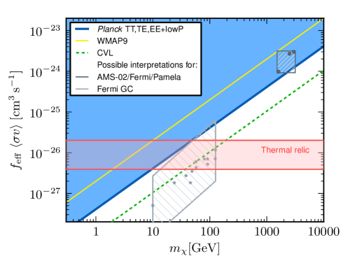
Figure 41 shows the constraints from WMAP9, Planck TT,TE,EE+lowP, and a forecast for a cosmic-variance-limited experiment with similar angular resolution to Planck.363636We assumed here that the cosmic-variance-limited experiment would measure the angular power spectra up to a maximum multipole of , observing a sky fraction . The horizontal red band includes the values of the thermal-relic cross-section multiplied by the appropriate for different DM annihilation channels. For example, the upper red line corresponds to , which is appropriate for a DM particle of mass annihilating into , while the lower red line corresponds to , for a DM particle annihilating into through an intermediate mediator (see, e.g., Arkani-Hamed et al. 2009). The Planck data exclude at 95 % confidence level a thermal relic cross-section for DM particles of mass annihilating into (), annihilating into or (), and annihilating into ().
The dark grey shaded area in Fig. 41 shows the approximate allowed region of parameter space, as calculated by Cholis & Hooper (2013) on the assumption that the PAMELA, AMS, and Fermi cosmic-ray excesses are caused by DM annihilation; the dark grey dots indicate the best-fit dark matter models described in that paper (for a recent discussion on best-fitting models, see also Boudaud et al. 2015). The favoured value of the cross-section is about two orders of magnitude higher than the thermal relic cross-section (). Attempts to reconcile such a high cross-section with the relic abundance of DM include a Sommerfeld enhanced cross-section (that may saturate at ) or non-thermal production of DM (see, e.g., the discussion by Madhavacheril et al. 2014). Both of these possibilities are strongly disfavoured by the Planck data. We cannot, however, exclude more exotic possibilities, such as DM annihilation through a p-wave channel with a cross-section that scales as (Diamanti et al. 2014). Since the relative velocity of DM particles at recombination is many orders of magnitude smaller than in the Galactic halo, such a model cannot be constrained using CMB data.
Observations from the Fermi Large Area Telescope of extended -ray emission towards the centre of the Milky Way, peaking at energies of around 1–3 GeV, have been interpreted as evidence for annihilating DM (e.g., Goodenough & Hooper 2009; Gordon & Macías 2013; Daylan et al. 2016; Abazajian et al. 2014; Lacroix et al. 2014). The light grey stars in Fig. 41 show specific models of DM annihilation designed to fit the Fermi -ray excess (Calore et al. 2015), while the light grey box shows the uncertainties of the best-fit cross-sections due to imprecise knowledge of the Galactic DM halo profile. Although the interpretation of the Fermi excess remains controversial (because of uncertainties in the astrophysical backgrounds), DM annihilation remains a possible explanation. The best-fit models of Calore et al. (2015) are consistent with the Planck constraints on DM annihilation.
6.7 Testing recombination physics with Planck
The cosmological recombination process determines how CMB photons decoupled from baryons around redshift , when the Universe was about 400 000 years old. The importance of this transition on the CMB anisotropies has long been recognized (Sunyaev & Zeldovich 1970; Peebles & Yu 1970). The most advanced computations of the ionization history (e.g., Ali-Haïmoud & Hirata 2010; Chluba & Thomas 2011; Ali-Haimoud & Hirata 2011; Chluba et al. 2012) account for many subtle atomic physics and radiative transfer effects that were not included in the earliest calculations (Zeldovich et al. 1968; Peebles 1968).
With precision data from Planck, we are sensitive to sub-percent variations of the free electron fraction around last-scattering (e.g., Hu et al. 1995; Seager et al. 2000; Seljak et al. 2003). Quantifying the impact of uncertainties in the ionization history around the maximum of the Thomson visibility function on predictions of the CMB power spectra is thus crucial for the scientific interpretation of data from Planck. In particular, for tests of models of inflation and extensions to , the interpretation of the CMB data can be significantly compromised by inaccuracies in the recombination calculation (e.g., Wong et al. 2008; Rubiño-Martín et al. 2010; Shaw & Chluba 2011). This problem can be approached in two ways, either by using modified recombination models with a specific physical process (or parameter) in mind, or in a semi-blind, model-independent way. Both approaches provide useful insights in assessing the robustness of the results from Planck.
Model-dependent limits on varying fundamental constants (Kaplinghat et al. 1999; Scóccola et al. 2009; Galli et al. 2009), annihilating or decaying particles (e.g., Chen & Kamionkowski 2004; Padmanabhan & Finkbeiner 2005; Zhang et al. 2006, and Sect. 6.6), or more general sources of extra ionization and excitation photons (Peebles et al. 2000; Doroshkevich et al. 2003; Galli et al. 2008), have been discussed extensively in the literature.
As already discussed in PCP13, the choice for Planck has been to use the rapid calculations of the recfast code, modified using corrections calculated with the more precise codes. To start this sub-section we quantify the effect on the analysis of Planck data of the remaining uncertainties in the standard recombination history obtained with different recombination codes (Sect. 6.7.1). We also derive CMB anisotropy-based measurements of the hydrogen – two-photon decay rate, (Sect. 6.7.2), and the average CMB temperature, derived at the last-scattering epoch (Sect. 6.7.3). These two parameters strongly affect the recombination history but are usually kept fixed when fitting models to CMB data (as in the analyses described in previous sections). Section 6.7.4 describes model-independent constraints on perturbed recombination scenarios. A discussion of these cases provides both a test of the consistency of the CMB data with the standard recombination scenario and also a demonstration of the impressive sensitivity of Planck to small variations in the ionization history at .
6.7.1 Comparison of different recombination codes
Even for pre-Planck data, it was realized that the early recombination calculations of Zeldovich et al. (1968) and Peebles (1968) had to be improved. This led to the development of the widely-used and computationally quick recfast code (Seager et al. 1999, 2000). However, for Planck, the recombination model of recfast in its original form is not accurate enough. Percent-level corrections, due to detailed radiative transfer and atomic physics effects have to be taken into account. Ignoring these effects can bias the inferred cosmological parameters, some by as much as a few standard deviations.
The recombination problem was solved as a common effort of several groups (Dubrovich & Grachev 2005; Kholupenko et al. 2007; Chluba & Sunyaev 2006b; Rubiño-Martín et al. 2006; Karshenboim & Ivanov 2008; Wong & Scott 2007; Switzer & Hirata 2008; Grin & Hirata 2010; Ali-Haïmoud & Hirata 2010). This work was undertaken, to a large extent, in preparation for the precision data from Planck. Both CosmoRec (Chluba & Thomas 2011) and HyRec (Ali-Haimoud & Hirata 2011) allow fast and precise computations of the ionization history, explicitly capturing the physics of the recombination problem. For the standard cosmology, the ionization histories obtained from these two codes in their default settings agree to within 0.05 % for hydrogen recombination () and 0.35 % during helium recombination373737Helium recombination is treated in more detail by CosmoRec (e.g., Rubiño-Martín et al. 2008; Chluba et al. 2012), which explains most of the difference. (). The effect of these small differences on the CMB power spectra is at and so has a negligible impact on the interpretation of precision CMB data; for the standard six parameters of base , we find that the largest effect is a bias in at the level of for Planck TT,TE,EE+lowP+BAO.
For Planck analyses, the recombination model of recfast is used by default. In recfast, the precise dynamics of recombination is not modelled physically, but approximated with fitting-functions calibrated against the full recombination calculations assuming a reference cosmology (Seager et al. 1999, 2000; Wong et al. 2008). At the level of precision required for Planck, the recfast approach is sufficiently accurate, provided that the cosmologies are close to base (Rubiño-Martín et al. 2010; Shaw & Chluba 2011). Comparing the latest version of recfast (camb version) with CosmoRec, we find agreement to within 0.2 % for hydrogen recombination () and 0.2 % during helium recombination for the standard ionization history. The effect on the CMB power spectra is at , although with slightly more pronounced shifts in the peak positions than when comparing CosmoRec and HyRec. For the base model, we find that the largest bias is on , at the level of () for Planck TT,TE,EE+lowP+BAO. Although this is about 5 times larger than the difference in between CosmoRec and HyRec, this bias is nevertheless unimportant at the current level of precision (and smaller than the differences seen from different likelihoods, see Sect. 3.1).
Finally we compare CosmoRec with recfast in its original form (i.e., before recalibrating the fitting-functions on refined recombination calculations). For base , we expect to see biases of and (Shaw & Chluba 2011). Using the actual data (Planck TT,TE,EE+lowP+BAO) we find biases of and , very close to the expected values. This illustrates explicitly the importance of the improvements of CosmoRec and HyRec over the original version of recfast for the interpretation of Planck data. However, CosmoRec and HyRec themselves are much more computationally intensive than the modified recfast, which is why we use recfast in most Planck cosmological analyses.
6.7.2 Measuring with Planck
The crucial role of the – two-photon decay channel for the dynamics of hydrogen recombination has been appreciated since the early days of CMB research (Zeldovich et al. 1968; Peebles 1968). Recombination is an out-of-equilibrium process and energetic photons emitted in the far Wien tail of the CMB by Lyman continuum and series transitions keep the primordial plasma ionized for a much longer period than expected from simple equilibrium recombination physics. Direct recombinations to the ground state of hydrogen are prohibited, causing a modification of the free electron number density, , by only around (Chluba & Sunyaev 2007). Similarly, the slow escape of photons from the Ly resonance reduces the effective Ly- transition rate to –10 s-1 (by more than seven orders of magnitude), making it comparable to the vacuum – two-photon decay rate of . About of all hydrogen atoms in the Universe became neutral through the – channel (e.g., Wong et al. 2006; Chluba & Sunyaev 2006a), and subtle effects, such as the induced – two-photon decay and Ly re-absorption, need to be considered in precision recombination calculations (Chluba & Sunyaev 2006b; Kholupenko & Ivanchik 2006; Hirata 2008).
The high sensitivity of the recombination process to the – two-photon transition rate also implies that instead of simply adopting a value for from theoretical computations (Breit & Teller 1940; Spitzer & Greenstein 1951; Goldman 1989) one can directly determine it with CMB data. From the theoretical point of view it would be surprising to find a value that deviates significantly from , derived from the most detailed computation (Labzowsky et al. 2005). However, laboratory measurements of this transition rate are extremely challenging (O’Connell et al. 1975; Krüger & Oed 1975; Cesar et al. 1996). The most stringent limit is for the differential decay rate, (a error) at wavelengths –, consistent with the theoretical value of in the same wavelength range (Krüger & Oed 1975). With precision data from Planck we are in a position to perform the best measurement to date, using cosmological data to inform us about atomic transition rates at last scattering (as also emphasized by Mukhanov et al. 2012).
The – two-photon rate affects the CMB anisotropies only through its effect on the recombination history. A larger value of , accelerates recombination, allowing photons and baryons to decouple earlier, an effect that shifts the acoustic peaks towards smaller scales. In addition, slightly less damping occurs, as in the case of the stimulated – two-photon decays (Chluba & Sunyaev 2006b). This implies that for flat cosmologies, variations of correlate with and (which affect the distance to the last scattering surface), while anti-correlates with and (which modify the slope of the damping tail). Despite these degeneracies, one expects that Planck will provide a measurement of to within , corresponding to an approximately 6 % uncertainty (Mukhanov et al. 2012).
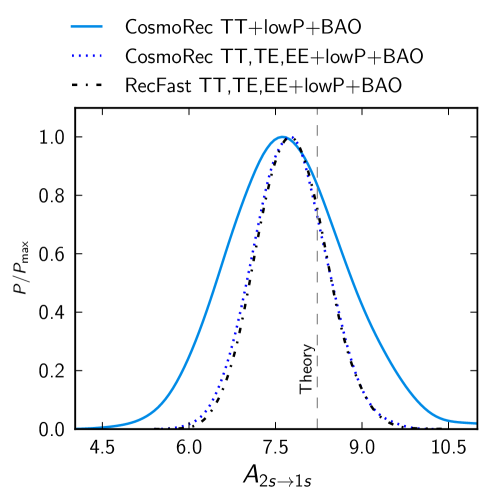
In Fig. 42, we show the marginalized posterior for from Planck and for Planck combined with BAO. Using CosmoRec to compute the recombination history, we find
| (0a) | |||||
| (0b) | |||||
| (0c) | |||||
| (0d) | |||||
These results are in very good agreement with the theoretical value, . For Planck TT,TE,EE+lowP+BAO, approximately 8 % precision is reached using cosmological data. These constraints are not sensitive to the addition of BAO, or other external data (JLA+). The slight shift away from the theoretical value is accompanied by small (fractions of a ) shifts in , , and , to compensate for the effects of on the distance to the last scattering surface and damping tail. This indicates that additional constraints on the acoustic scale are required to fully break degeneracies between these parameters and their effects on the CMB power spectrum, a task that could be achieved in the future using large-scale structure surveys and next generation CMB experiments.
The values for quoted above were obtained using CosmoRec. When varying , the range of cosmologies becomes large enough to potentially introduce a mismatch of the recfast fitting-functions that could affect the posterior. In particular, with recfast the – two-photon and Ly channels are not treated separately, so that changes specific to the – decay channel propagate inconsistently.383838One effect is that by increasing fewer Ly photons are produced. This reduces the Ly feedback correction to the – channel, which further accelerates recombination, an effect that is not captured with recfast in the current implementation. However, repeating the analysis with recfast, we find (see Fig. 42), for Planck TT,TE,EE+lowP+BAO, which is in excellent agreement with CosmoRec, showing that these effects can be neglected.
6.7.3 Measuring at last-scattering with Planck
Our best constraint on the CMB monopole temperature comes from the measurements of the CMB spectrum with COBE/FIRAS, giving a determination of (Fixsen et al. 1996; Fixsen 2009). Other constraints from molecular lines typically reach precision (see table 2 in Fixsen 2009, for an overview), while independent BBN constraints provide 5–10 % limits (Simha & Steigman 2008; Jeong et al. 2014).
The CMB anisotropies provide additional ways of determining the value of (for fixed values of and ). One is through the energy distribution of the CMB anisotropies (Fixsen et al. 1996; Fixsen 2003; Chluba 2014) and another through their power spectra (Opher & Pelinson 2004, 2005; Chluba 2014). Even small changes in , compatible with the COBE/FIRAS error, affect the ionization history at the 0.5 % level around last-scattering, propagating to a roughly 0.1 % uncertainty in the CMB power spectrum (Chluba & Sunyaev 2008). Overall, the effect of this uncertainty on the parameters of models is small (Hamann & Wong 2008); however, without prior knowledge of from the COBE/FIRAS measurement, the situation would change significantly.
The CMB monopole affects the CMB anisotropies in several ways. Most importantly, for larger , photons decouple from baryons at lower redshift, since more ionizing photons are present in the Wien-tail of the CMB. This effect is amplified because of the exponential dependence of the atomic level populations on the ratio of the ionization potentials and CMB temperature. In addition, increasing lowers the expansion timescale of the Universe and the redshift of matter-radiation equality, while increasing the photon sound speed. Some of these effects are also produced by varying ; however, the effects of on the ionization history and photon sound speed are distinct.
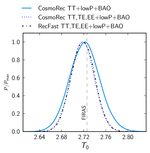
With CMB data alone, the determination of is degenerate with other parameters, but the addition of other data sets breaks this degeneracy. Marginalized posterior distributions for are shown in Fig. 43. Using CosmoRec, we find
| (0a) | |||||
| (0b) |
and similar results are obtained with recfast. This is in excellent agreement with the COBE/FIRAS measurement, (Fixsen et al. 1996; Fixsen 2009). These measurements of reach a precision that is comparable to the accuracy obtained with interstellar molecules. Since the systematics of these independent methods are very different, this result demonstrates the consistency of all these data. Allowing to vary causes the errors of the other cosmological parameters to increase. The strongest effect is on , which is highly degenerate with . The error on increases by a factor of roughly if is allowed to vary. The error on increases by a factor of about 4, while the errors on and increase by factors of 1.5–2, and the other cosmological parameters are largely unaffected by variations in . Because of the strong degeneracy with , no constraint on can be obtained using Planck data alone. External data, such as BAO, are therefore required to break this geometric degeneracy.
It is important to emphasize that the CMB measures the temperature at a redshift of , so the comparison with measurements of at the present day is effectively a test of the constancy of , where is the scale-factor at the time of last-scattering. It is remarkable that we are able to test the constancy of over such a large dynamic range in redshift. Of course, if we did find that around recombination were discrepant with now, then we would need to invent a finely-tuned late-time photon injection mechanism393939Pure energy release in the form of heating of ordinary matter would leave a Compton -distortion (Zeldovich & Sunyaev 1969) at these late times (Burigana et al. 1991; Hu & Silk 1993; Chluba & Sunyaev 2012). to explain the anomaly. Fortunately, the data are consistent with the standard scaling of the CMB temperature.
Another approach to measuring is through the thermal Sunyaev-Zeldovich effect in rich clusters of galaxies at various redshifts (Fabbri et al. 1978; Rephaeli 1980), although it is unclear how one would interpret a failure of this test without an explicit model. In practice this approach is consistent with a scaling , but with lower precision than obtained here from Planck (e.g., Battistelli et al. 2002; Luzzi et al. 2009; Saro et al. 2014; Hurier et al. 2014). A simple modification to the standard temperature redshift relation is frequently discussed in the literature (though this case is not justified by any physical model and is difficult to realize without creating a CMB spectral distortion, see Chluba 2014). For this parameterization we find
| (0a) | |||||
| (0b) |
where we have adopted a recombination redshift of .404040The test depends on the logarithm of the redshift and so is insensitive to the precise value adopted for . Because of the long lever-arm in redshift afforded by the CMB, this is an improvement over earlier constraints by more than an order of magnitude (e.g., Hurier et al. 2014).
In a self-consistent picture, changes of would also affect the BBN era. We might therefore consider a simultaneous variation of and to reflect the variation of the neutrino energy density accompanying a putative variation in the photon energy density. Since we find at recombination to be highly consistent with the observed CMB temperature from COBE/FIRAS, considering this extra variation seems unnecessary. Instead, we may view the variation investigated here as further support for the limits discussed in Sects. 6.4 and 6.5.
6.7.4 Semi-blind perturbed recombination analysis
The high sensitivity of small-scale CMB anisotropies to the ionization history of the Universe around the epoch of recombination allows us to constrain possible deviations from the standard recombination scenario in a model-independent way (Farhang et al. 2012, 2013). The method relies on an eigen-analysis (often referred to as a principle component analysis) of perturbations in the free electron fraction, , where denotes the number density of hydrogen nuclei. The eigenmodes selected are specific to the data used in the analysis. Similar approaches have been used to constrain deviations of the reionization history from the simplest models (Mortonson & Hu 2008) and annihilating dark matter scenarios (Finkbeiner et al. 2012), both with the prior assumption that the standard recombination physics is fully understood, as well as for constraining trajectories in inflation Planck Collaboration XX (2016) and dark energy Planck Collaboration XIV (2016) parameterizations.
Here, we use Planck data to find preferred ionization fraction trajectories composed of low-order perturbation eigenmodes to the standard history (-modes). The -modes are constructed through the eigen-decomposition of the inverse of the Fisher information matrix for base (the six cosmological parameters and the nuisance parameters) and recombination perturbation parameters (see Farhang et al. 2012, for details). This procedure allows us to estimate the errors on the eigenmode amplitudes, , providing a rank ordering of the -modes and their information content.
The first three -modes for Planck TT,TE,EE+lowP are illustrated in Fig. 44, together with their impact on the differential visibility function. Figure 45 shows the response of the CMB temperature and polarization power spectra to these eigenmodes. The first mode mainly leads to a change in the width and height of the Thomson visibility function (bottom panel of Fig. 44). This implies less diffusion damping, which is also reflected in the modifications to the CMB power spectra (as shown in Fig. 45). The second mode causes the visibility maximum to shift towards higher redshifts for , which leads to a shift of the CMB extrema to smaller scales; however, for roughly constant width of the visibility function it also introduces less damping at small scales. The third mode causes a combination of changes in both the position and width of the visibility function, with a pronounced effect on the location of the acoustic peaks. For the analysis of Planck data combinations, we only use -modes that are optimized for Planck TT,TE,EE+lowP.
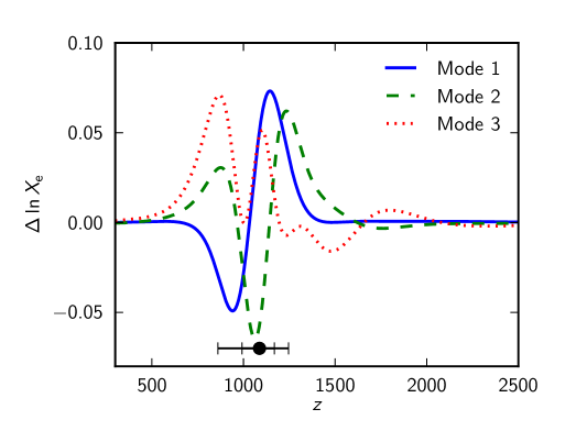
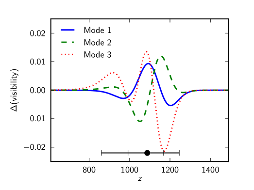
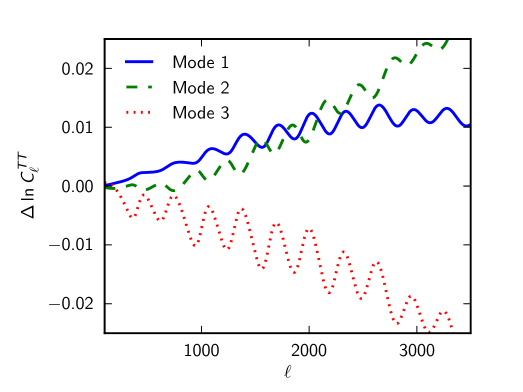
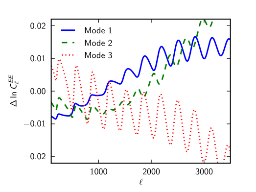
We modified CosmoMC to estimate the mode amplitudes. The results for Planck TT,TE,EE+lowP+BAO are presented in Table 7. Although all mode amplitudes are consistent with standard recombination, adding the second -mode causes mild shifts in and . For Planck TT+lowP, we find and , using the Planck TT,TE,EE+lowP eigenmodes, again consistent with the standard recombination scenario. Adding the polarization data improves the errors by more than a factor of 2. However, the mode amplitudes are insensitive to the addition of external data.
|
With pre-Planck data, only the amplitude, , of the first eigenmode could be constrained. The corresponding change in the ionization history translates mainly into a change in the slope of the CMB damping tail, with this mode resembling the first mode determined using Planck data (Fig. 44). The WMAP9+SPT data gave a non-zero value for the first eigenmode at about , . However, the WMAP9+ACT data gave and the combined pre-Planck data (WMAP+ACT+SPT) gave , both consistent with the standard recombination scenario (Calabrese et al. 2013). The variation among these results is another manifestation of the tensions between different pre-Planck CMB data, as discussed in PCP13.
Although not optimal for Planck data, we also compute the amplitudes of the first three -modes constructed for the WMAP9+SPT data set. This provides a more direct comparison with the pre-Planck constraints. For Planck TT,TE,EE+lowP+BAO we obtain and . The mild tension of the pre-Planck data with the standard recombination scenario disappears when using Planck data. This is especially impressive, since the errors have improved by more than a factor of 2. By projecting onto the Planck modes, we find that the first two SPT modes can be expressed as and , which emphasizes the consistency of the results. Adding the first three SPT modes, we obtain , , and , which again is consistent with the standard model of recombination. The small changes in the mode amplitudes when adding the third mode arise because the SPT modes are not optimal for Planck and so are correlated.
6.8 Cosmic defects
Topological defects are a generic by-product of symmetry-breaking phase transitions and a common phenomenon in condensed matter systems. Cosmic defects of various types can be formed in phase transitions in the early Universe (Kibble 1976). In particular, cosmic strings can be produced in some supersymmetric and grand-unified theories at the end of inflation (Jeannerot et al. 2003), as well as in higher-dimensional theories (e.g., Polchinski 2005). Constraints on the abundance of cosmic strings and other defects therefore place limits on a range of models of the early Universe. More discussion on the formation, evolution, and cosmological role of topological defects can be found, for example, in the reviews by Vilenkin & Shellard (2000), Hindmarsh & Kibble (1995), and Copeland & Kibble (2010).
In this section we revisit the power spectrum-based constraints on the abundance of cosmic strings and other topological defects using the 2015 Planck data, including Planck polarization measurements. The general approach follows that described in the Planck 2013 analysis of cosmic defects (Planck Collaboration XXV 2014), so here we focus on the updated constraints rather than on details of the methodology.
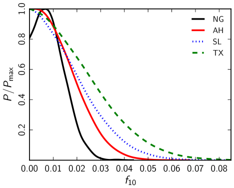
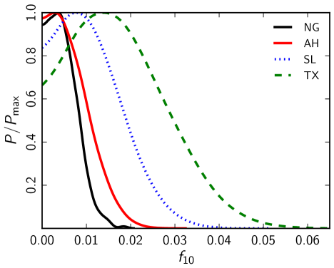
Topological defects are non-perturbative excitations of the underlying field theory and their study requires numerical simulations. Unfortunately, since the Hubble scale, , is over 50 orders of magnitude greater that the thickness of a GUT-scale string, approximately with the mass per unit length of the string, it is impractical to simulate the string dynamics exactly in the late Universe. For this reason one needs to make approximations. One approach considers the limit of an infinitely thin string, which corresponds to using the Nambu-Goto (“NG”) action for the string dynamics. In an alternative approach, the actual field dynamics for a given model are solved on a lattice. In this case it is necessary to resolve the string core, which generally requires more computationally intensive simulations than in the NG approach. Lattice simulations, however, can include additional physics, such as field radiation that is not present in NG simulations. Here we will use field-theory simulations of the Abelian-Higgs action (“AH”); details of these simulations are discussed in Bevis et al. (2007, 2010).
The field-theory approach also allows one to simulate theories in which the defects are not cosmic strings and so cannot be described by the NG action. Examples include semi-local strings (“SL”, Urrestilla et al. 2008) and global defects. Here we will specifically consider the breaking of a global symmetry resulting in texture defects (“TX”).
For the field-theory defects, we measure the energy-momentum tensor from the simulations and insert it as an additional constituent into a modified version of the CMBEASY Boltzmann code (Doran 2005) to predict the defect contribution to the CMB temperature and polarization power spectra (see, e.g., Durrer et al. 2002). The same approach can be applied to NG strings, but rather than using simulations directly, we model the strings using the unconnected segment model (“USM”, Albrecht et al. 1999; Pogosian & Vachaspati 1999). In this model, strings are represented by a set of uncorrelated straight segments, with scaling properties chosen to match those determined from numerical simulations. In this case, the string energy-momentum tensor can be computed analytically and used as an active source in a modified Boltzmann code. For this analysis we use CMBACT version 4,414141http://www.sfu.ca/~levon/cmbact.html whereas Planck Collaboration XXV (2014) used version 3. There have been several improvements to the code since the 2013 analysis, including a correction to the normalization of vector mode spectra. However, the largest change comes from an improved treatment of the scaling properties. The string correlation length and velocity are described by an updated velocity-dependent one-scale model (Martins & Shellard 2002), which provides better agreement with numerical simulations. Small-scale structure of the string, which was previously a free parameter, is accounted for by the one-scale model.
The CMB power spectra from defects are proportional to . We scale the computed template CMB spectra, and add these to the inflationary and foreground power spectra, to form the theory spectra that enter the likelihood. In practice, we parameterize the defects with their relative contribution to the spectrum at multipole , . We vary and the standard six parameters of the base model, using CosmoMC. We also report our results in terms of the derived parameter .
|
||||||||||||||||||||||||||||||||
The constraints on and the inferred limits on are summarized in Table 8. The marginalized 1D posterior distribution functions are shown in Fig. 46. For Planck TT+lowP we find that the results are similar to the Planck+WP constraints reported in Planck Collaboration XXV (2014), for the AH model, or somewhat better for SL and TX. However, the addition of the Planck high- and polarization data leads to a significant improvement compared to the 2013 constraints.
For the NG string model, the results based on Planck TT+lowP are slightly weaker than the 2013 Planck+WP constraints. This is caused by a difference in the updated defect spectrum from the USM model, which has a less pronounced peak and shifts towards the AH spectrum. With the inclusion of polarization, Planck TT,TE,EE+lowP improves the upper limit on by a factor of 2, as for the AH model. The differences between the AH and NG results quoted here can be regarded as a rough indication of the uncertainty in the theoretical string power spectra.
In summary, we find no evidence for cosmic defects from the Planck 2015 data, with tighter limits than before.
7 Conclusions424242As in the abstract, here we quote 68 % confidence limits on measured parameters and 95 % upper limits on other parameters.
(1)
The six-parameter base model continues to provide a very good match to the more extensive 2015 Planck data, including polarization. This is the most important conclusion of this paper.
(2)
The 2015 Planck , , , and lensing spectra are consistent with each other under the assumption of the base cosmology. However, when comparing the and spectra computed for different frequency combinations, we find evidence for systematic effects caused by temperature-to-polarization leakage. These effects are at low levels and have little impact on the science conclusions of this paper.
(3)
We have presented the first results on polarization from the LFI at low multipoles. The LFI polarization data, together with Planck lensing and high-multipole temperature data, gives a reionization optical depth of and a reionization redshift of . These numbers are in good agreement with those inferred from the WMAP9 polarization data cleaned for polarized dust emission using HFI 353-GHz maps. They are also in good agreement with results from Planck temperature and lensing data, i.e., excluding any information from polarization at low multipoles.
(4)
The absolute calibration of the Planck 2015 HFI spectra is higher by (in power) compared to 2013, largely resolving the calibration difference noted in PCP13 between WMAP and Planck. In addition, there have been a number of small changes to the low-level Planck processing and more accurate calibrations of the HFI beams. The 2015 Planck likelihood also makes more aggressive use of sky than in PCP13 and incorporates some refinements to the modelling of unresolved foregrounds. Apart from differences in (caused by switching to the LFI low-multipole polarization likelihood, as described in item 3 above) and the amplitude- combination (caused by the change in absolute calibration), the 2015 parameters for base are in good agreement with those reported in PCP13.
(5)
The Planck , , and spectra are accurately described by a purely adiabatic spectrum of fluctuations with a spectral tilt , consistent with the predictions of single-field inflationary models. Combining Planck data with BAO, we find tight limits on the spatial curvature of the Universe, , again consistent with the inflationary prediction of a spatially-flat Universe.
(6)
The Planck data show no evidence for tensor modes. Adding a tensor amplitude as a one-parameter extension to base , we derive a 95 % upper limit of . This is consistent with the -mode polarization analysis reported in BKP, resolving the apparent discrepancy between the Planck constraints on and the BICEP2 results reported by BICEP2 Collaboration (2014). In fact, by combining the Planck and BKP likelihoods, we find an even tighter constraint, , strongly disfavouring inflationary models with a potential.
(7)
The Planck data show no evidence for any significant running of the spectral index. We also set strong limits on a possible departure from a purely adiabatic spectrum, either through an admixture of fully-correlated isocurvature modes or from cosmic defects.
(8)
The Planck best-fit base cosmology (we quote numbers for Planck TT+lowP+lensing here) is in good agreement with results from BAO surveys, and with the recent JLA sample of Type Ia SNe. The Hubble constant in this cosmology is , consistent with the direct measurement of of Eq. (1) used as an prior in this paper. The Planck base cosmology is also consistent with the recent analysis of redshift-space distortions of the BOSS CMASS-DR11 data by Samushia et al. (2014) and Beutler et al. (2014). The amplitude of the present-day fluctuation spectrum, , of the Planck base cosmology is higher than inferred from weak lensing measurements from the CFHTLenS survey (Heymans et al. 2012; Erben et al. 2013) and, possibly, from counts of rich clusters of galaxies (including Planck cluster counts reported in Planck Collaboration XXIV 2016). The Planck base cosmology is also discordant with Ly BAO measurements at (Delubac et al. 2015; Font-Ribera et al. 2014). At present, the reasons for these tensions are unclear.
(9)
By combining the Planck TT+lowP+lensing data with other astrophysical data, including the JLA supernovae, the equation of state for dark energy is constrained to and is therefore compatible with a cosmological constant, as assumed in the base cosmology.
(10)
We have presented a detailed analysis of possible extensions to the neutrino sector of the base model. Combining Planck TT+lowP+lensing with BAO we find for the effective number of relativistic degrees of freedom, consistent with the value of the standard model. The sum of neutrino masses is constrained to . The Planck data strongly disfavour fully thermalized sterile neutrinos with that have been proposed as a solution to reactor neutrino oscillation anomalies. From Planck, we find no evidence for new neutrino physics. Standard neutrinos with masses larger than those in the minimal mass hierarchy are still allowed, and could be detectable in combination with future astrophysical and CMB lensing data.
(11)
The standard theory of big bang nucleosynthesis, with and negligible leptonic asymmetry in the electron neutrino sector, is in excellent agreement with Planck data and observations of primordial light element abundances. This agreement is particularly striking for deuterium, for which accurate primordial abundance measurements have been reported recently (Cooke et al. 2014). The BBN theoretical predictions for deuterium are now dominated by uncertainties in nuclear reaction rates (principally the radiative capture process), rather than from Planck uncertainties in the physical baryon density .
(12)
We have investigated the temperature and polarization signatures associated with annihilating dark matter and possible deviations from the standard recombination history. Again, we find no evidence for new physics from the Planck data.
In summary, the Planck temperature and polarization spectra presented in Figs. 1 and 3 are more precise (and accurate) than those from any previous CMB experiment, and improve on the 2013 spectra presented in PCP13. Yet we find no signs for any significant deviation from the base cosmology. Similarly, the analysis of 2015 Planck data reported in Planck Collaboration XVII (2016) sets unprecedentedly tight limits on primordial non-Gaussianity. The Planck results offer powerful evidence in favour of simple inflationary models, which provide an attractive mechanism for generating the slightly tilted spectrum of (nearly) Gaussian adiabatic perturbations that match our data to such high precision. In addition, the Planck data show that the neutrino sector of the theory is consistent with the assumptions of the base model and that the dark energy is compatible with a cosmological constant. If there is new physics beyond base , then the corresponding observational signatures in the CMB are weak and difficult to detect. This is the legacy of the Planck mission for cosmology.
Acknowledgements.
The Planck Collaboration acknowledges the support of: ESA; CNES and CNRS/INSU-IN2P3-INP (France); ASI, CNR, and INAF (Italy); NASA and DoE (USA); STFC and UKSA (UK); CSIC, MINECO, JA, and RES (Spain); Tekes, AoF, and CSC (Finland); DLR and MPG (Germany); CSA (Canada); DTU Space (Denmark); SER/SSO (Switzerland); RCN (Norway); SFI (Ireland); FCT/MCTES (Portugal); ERC and PRACE (EU). A description of the Planck Collaboration and a list of its members, indicating which technical or scientific activities they have been involved in, can be found at http://www.cosmos.esa.int/web/planck/planck-collaboration. Some of the results in this paper have been derived using the HEALPix package. The research leading to these results has received funding from the European Research Council under the European Union’s Seventh Framework Programme (FP/2007–2013) / ERC Grant Agreement No. [616170] and from the UK Science and Technology Facilities Council [grant number ST/L000652/1]. Part of this work was undertaken on the STFC DiRAC HPC Facilities at the University of Cambridge, funded by UK BIS National E-infrastructure capital grants, and on the Andromeda cluster of the University of Geneva. A large set of cosmological parameter constraints from different data combinations, and including many separate extensions to the 6-parameter base model, are available at http://pla.esac.esa.int/pla/#cosmology.References
- Abazajian et al. (2015a) Abazajian, K. et al., Inflation Physics from the Cosmic Microwave Background and Large Scale Structure. 2015a, Astropart. Phys., 63, 55, 1309.5381
- Abazajian et al. (2015b) Abazajian, K. et al., Neutrino Physics from the Cosmic Microwave Background and Large Scale Structure. 2015b, Astropart. Phys., 63, 66, 1309.5383
- Abazajian et al. (2012) Abazajian, K. N., Acero, M. A., Agarwalla, S. K., et al., Light Sterile Neutrinos: A White Paper. 2012, ArXiv e-prints, 1204.5379
- Abazajian et al. (2014) Abazajian, K. N., Canac, N., Horiuchi, S., & Kaplinghat, M., Astrophysical and Dark Matter Interpretations of Extended Gamma-Ray Emission from the Galactic Center. 2014, Phys. Rev., D90, 023526, 1402.4090
- Ackermann et al. (2012) Ackermann, M., Ajello, M., Allafort, A., et al., Measurement of Separate Cosmic-Ray Electron and Positron Spectra with the Fermi Large Area Telescope. 2012, Phys. Rev. Lett., 108, 011103, 1109.0521
- Ackermann et al. (2014) Ackermann, M. et al., Dark matter constraints from observations of 25 Milky Way satellite galaxies with the Fermi Large Area Telescope. 2014, Phys. Rev., D89, 042001, 1310.0828
- Addison et al. (2012) Addison, G. E., Dunkley, J., & Spergel, D. N., Modelling the correlation between the thermal Sunyaev Zel’dovich effect and the cosmic infrared background. 2012, MNRAS, 427, 1741, 1204.5927
- Ade et al. (2014) Ade, P. A. R. et al., Measurement of the Cosmic Microwave Background Polarization Lensing Power Spectrum with the POLARBEAR experiment. 2014, Phys. Rev. Lett., 113, 021301, 1312.6646
- Adelberger et al. (2011) Adelberger, E., Balantekin, A., Bemmerer, D., et al., Solar fusion cross sections II: the pp chain and CNO cycles. 2011, Rev. Mod. Phys., 83, 195, 1004.2318
- Adriani et al. (2009) Adriani, O., Barbarino, G. C., Bazilevskaya, G. A., et al., An anomalous positron abundance in cosmic rays with energies 1.5-100GeV. 2009, Nature, 458, 607, 0810.4995
- Aguilar et al. (2014) Aguilar, M., Aisa, D., Alvino, A., et al., Electron and Positron Fluxes in Primary Cosmic Rays Measured with the Alpha Magnetic Spectrometer on the International Space Station. 2014, Phys. Rev. Lett., 113, 121102
- Albrecht et al. (1999) Albrecht, A., Battye, R. A., & Robinson, J., Detailed study of defect models for cosmic structure formation. 1999, Phys. Rev., D59, 023508, astro-ph/9711121
- Alcock & Paczynski (1979) Alcock, C. & Paczynski, B., An evolution free test for non-zero cosmological constant. 1979, Nature, 281, 358
- Ali-Haïmoud & Hirata (2010) Ali-Haïmoud, Y. & Hirata, C. M., Ultrafast effective multilevel atom method for primordial hydrogen recombination. 2010, Phys. Rev., D82, 063521, 1006.1355
- Ali-Haimoud & Hirata (2011) Ali-Haimoud, Y. & Hirata, C. M., HyRec: A fast and highly accurate primordial hydrogen and helium recombination code. 2011, Phys. Rev., D83, 043513, 1011.3758
- Amendola et al. (2002) Amendola, L., Gordon, C., Wands, D., & Sasaki, M., Correlated perturbations from inflation and the cosmic microwave background. 2002, Phys. Rev. Lett., 88, 211302, astro-ph/0107089
- Anders et al. (2014) Anders, M., Trezzi, D., Menegazzo, R., et al., First Direct Measurement of the H2( ,)Li6 Cross Section at Big Bang Energies and the Primordial Lithium Problem. 2014, Phys. Rev. Lett., 113, 042501
- Anderson et al. (2014) Anderson, L., Aubourg, É., Bailey, S., et al., The clustering of galaxies in the SDSS-III Baryon Oscillation Spectroscopic Survey: baryon acoustic oscillations in the Data Releases 10 and 11 Galaxy samples. 2014, MNRAS, 441, 24, 1312.4877
- Anderson et al. (2012) Anderson, L., Aubourg, E., Bailey, S., et al., The clustering of galaxies in the SDSS-III Baryon Oscillation Spectroscopic Survey: baryon acoustic oscillations in the Data Release 9 spectroscopic galaxy sample. 2012, MNRAS, 427, 3435, 1203.6594
- Archidiacono et al. (2011) Archidiacono, M., Calabrese, E., & Melchiorri, A., The Case for Dark Radiation. 2011, Phys. Rev., D84, 123008, 1109.2767
- Archidiacono et al. (2013a) Archidiacono, M., Fornengo, N., Giunti, C., Hannestad, S., & Melchiorri, A., Sterile neutrinos: Cosmology versus short-baseline experiments. 2013a, Phys. Rev., D87, 125034, 1302.6720
- Archidiacono et al. (2013b) Archidiacono, M., Giusarma, E., Melchiorri, A., & Mena, O., Neutrino and dark radiation properties in light of recent CMB observations. 2013b, Phys. Rev., D87, 103519, 1303.0143
- Arkani-Hamed et al. (2009) Arkani-Hamed, N., Finkbeiner, D. P., Slatyer, T. R., & Weiner, N., A Theory of Dark Matter. 2009, Phys. Rev., D79, 015014, 0810.0713
- Aubourg et al. (2015) Aubourg, E. et al., Cosmological implications of baryon acoustic oscillation measurements. 2015, Phys. Rev., D92, 123516, 1411.1074
- Audren et al. (2013) Audren, B., Lesgourgues, J., Benabed, K., & Prunet, S., Conservative constraints on early cosmology with MONTE PYTHON. 2013, J. Cosmology Astropart. Phys., 2, 001, 1210.7183
- Audren et al. (2015) Audren, B. et al., Robustness of cosmic neutrino background detection in the cosmic microwave background. 2015, JCAP, 1503, 036, 1412.5948
- Aver et al. (2013) Aver, E., Olive, K. A., Porter, R., & Skillman, E. D., The primordial helium abundance from updated emissivities. 2013, JCAP, 1311, 017, 1309.0047
- Bartelmann & Schneider (2001) Bartelmann, M. & Schneider, P., Weak gravitational lensing. 2001, Phys. Rep., 340, 291, astro-ph/9912508
- Bashinsky & Seljak (2004) Bashinsky, S. & Seljak, U., Neutrino perturbations in CMB anisotropy and matter clustering. 2004, Phys. Rev., D69, 083002, astro-ph/0310198
- Battistelli et al. (2002) Battistelli, E. S., De Petris, M., Lamagna, L., et al., Cosmic Microwave Background Temperature at Galaxy Clusters. 2002, ApJ, 580, L101, arXiv:astro-ph/0208027
- Battye et al. (2015) Battye, R. A., Charnock, T., & Moss, A., Tension between the power spectrum of density perturbations measured on large and small scales. 2015, Phys. Rev., D91, 103508, 1409.2769
- Battye & Moss (2014) Battye, R. A. & Moss, A., Evidence for massive neutrinos from CMB and lensing observations. 2014, Phys. Rev. Lett., 112, 051303, 1308.5870
- Beacom et al. (2004) Beacom, J. F., Bell, N. F., & Dodelson, S., Neutrinoless universe. 2004, Phys. Rev. Lett., 93, 121302, astro-ph/0404585
- Bean et al. (2006) Bean, R., Dunkley, J., & Pierpaoli, E., Constraining Isocurvature Initial Conditions with WMAP 3-year data. 2006, Phys. Rev., D74, 063503, astro-ph/0606685
- Bell (2005) Bell, N. F., Neutrino mixing and cosmology. 2005, Nucl. Phys. B Proc. Suppl., 138, 76, hep-ph/0311283
- Bennett et al. (2003) Bennett, C. L., Halpern, M., Hinshaw, G., et al., First-Year Wilkinson Microwave Anisotropy Probe (WMAP) Observations: Preliminary Maps and Basic Results. 2003, ApJS, 148, 1, arXiv:astro-ph/0302207
- Bennett et al. (2011) Bennett, C. L., Hill, R. S., Hinshaw, G., et al., Seven-year Wilkinson Microwave Anisotropy Probe (WMAP) Observations: Are There Cosmic Microwave Background Anomalies? 2011, ApJS, 192, 17, 1001.4758
- Bennett et al. (2014) Bennett, C. L., Larson, D., Weiland, J. L., & Hinshaw, G., The 1% Concordance Hubble Constant. 2014, ApJ, 794, 135, 1406.1718
- Bennett et al. (2013) Bennett, C. L., Larson, D., Weiland, J. L., et al., Nine-year Wilkinson Microwave Anisotropy Probe (WMAP) Observations: Final Maps and Results. 2013, ApJS, 208, 20, 1212.5225
- Benson et al. (2013) Benson, B. A., de Haan, T., Dudley, J. P., et al., Cosmological Constraints from Sunyaev-Zel’dovich-selected Clusters with X-Ray Observations in the First 178 deg2 of the South Pole Telescope Survey. 2013, ApJ, 763, 147, 1112.5435
- Bergström et al. (2014) Bergström, J., Gonzalez-Garcia, M. C., Niro, V., & Salvado, J., Statistical tests of sterile neutrinos using cosmology and short-baseline data. 2014, JHEP, 10, 104, 1407.3806
- Béthermin et al. (2012) Béthermin, M., Daddi, E., Magdis, G., et al., A Unified Empirical Model for Infrared Galaxy Counts Based on the Observed Physical Evolution of Distant Galaxies. 2012, ApJ, 757, L23, 1208.6512
- Betoule et al. (2013) Betoule, M., Marriner, J., Regnault, N., et al., Improved photometric calibration of the SNLS and the SDSS supernova surveys. 2013, A&A, 552, A124, 1212.4864
- Betoule et al. (2014) Betoule, M. et al., Improved cosmological constraints from a joint analysis of the SDSS-II and SNLS supernova samples. 2014, A&A, 1401.4064
- Betts et al. (2013) Betts, S. et al. 2013, in Community Summer Study 2013: Snowmass on the Mississippi (CSS2013) Minneapolis, MN, USA, July 29-August 6, 2013
- Beutler et al. (2011) Beutler, F., Blake, C., Colless, M., et al., The 6dF Galaxy Survey: baryon acoustic oscillations and the local Hubble constant. 2011, MNRAS, 416, 3017, 1106.3366
- Beutler et al. (2012) Beutler, F., Blake, C., Colless, M., et al., The 6dF Galaxy Survey: measurements of the growth rate and 8. 2012, MNRAS, 423, 3430, 1204.4725
- Beutler et al. (2014) Beutler, F., Saito, S., Seo, H.-J., et al., The clustering of galaxies in the SDSS-III Baryon Oscillation Spectroscopic Survey: testing gravity with redshift space distortions using the power spectrum multipoles. 2014, MNRAS, 443, 1065, 1312.4611
- Beutler et al. (2014) Beutler, F. et al., The clustering of galaxies in the SDSS-III Baryon Oscillation Spectroscopic Survey: Signs of neutrino mass in current cosmological datasets. 2014, MNRAS, 444, 3501, 1403.4599
- Bevis et al. (2007) Bevis, N., Hindmarsh, M., Kunz, M., & Urrestilla, J., CMB power spectrum contribution from cosmic strings using field-evolution simulations of the Abelian Higgs model. 2007, Phys. Rev., D75, 065015, astro-ph/0605018
- Bevis et al. (2010) Bevis, N., Hindmarsh, M., Kunz, M., & Urrestilla, J., CMB power spectra from cosmic strings: predictions for the Planck satellite and beyond. 2010, Phys. Rev., D82, 065004, 1005.2663
- Bianchi et al. (2012) Bianchi, D., Guzzo, L., Branchini, E., et al., Statistical and systematic errors in redshift-space distortion measurements from large surveys. 2012, MNRAS, 427, 2420, 1203.1545
- BICEP2 Collaboration (2014) BICEP2 Collaboration, Detection of B-Mode Polarization at Degree Angular Scales by BICEP2. 2014, Phys. Rev. Lett., 112, 241101, 1403.3985
- BICEP2/Keck Array and Planck Collaborations (2015) BICEP2/Keck Array and Planck Collaborations, Joint Analysis of BICEP2/Keck Array and Planck Data. 2015, Phys. Rev. Lett., 114, 101301, 1502.00612
- Blake et al. (2012) Blake, C., Brough, S., Colless, M., et al., The WiggleZ Dark Energy Survey: joint measurements of the expansion and growth history at . 2012, MNRAS, 425, 405, 1204.3674
- Blake et al. (2011) Blake, C., Kazin, E. A., Beutler, F., et al., The WiggleZ Dark Energy Survey: mapping the distance-redshift relation with baryon acoustic oscillations. 2011, MNRAS, 418, 1707, 1108.2635
- Böhringer et al. (2014) Böhringer, H., Chon, G., & Collins, C. A., The extended ROSAT-ESO Flux Limited X-ray Galaxy Cluster Survey (REFLEX II). IV. X-ray luminosity function and first constraints on cosmological parameters. 2014, A&A, 570, A31, 1403.2927
- Bond et al. (1997) Bond, J., Efstathiou, G., & Tegmark, M., Forecasting cosmic parameter errors from microwave background anisotropy experiments. 1997, MNRAS, 291, L33, astro-ph/9702100
- Boudaud et al. (2015) Boudaud, M. et al., A new look at the cosmic ray positron fraction. 2015, A&A, 575, A67, 1410.3799
- Bousso et al. (2015) Bousso, R., Harlow, D., & Senatore, L., Inflation after False Vacuum Decay. 2015, Phys. Rev., D91, 083527, 1309.4060
- Breit & Teller (1940) Breit, G. & Teller, E., Metastability of Hydrogen and Helium Levels. 1940, ApJ, 91, 215
- Bucher et al. (1995) Bucher, M., Goldhaber, A. S., & Turok, N., An open universe from inflation. 1995, Phys. Rev., D52, 3314, hep-ph/9411206
- Bucher et al. (2001a) Bucher, M., Moodley, K., & Turok, N., Constraining Isocurvature Perturbations with CMB Polarization. 2001a, Phys. Rev. Lett., 87, 191301, astro-ph/0012141
- Bucher et al. (2001b) Bucher, M., Moodley, K., & Turok, N., The General Primordial Cosmic Perturbation. 2001b, Phys. Rev., D62, 083508, astro-ph/9904231
- Buchmuller et al. (2013) Buchmuller, W., Domcke, V., & Kamada, K., The Starobinsky model from superconformal D-term inflation. 2013, Phys. Lett. B, 726, 467, 1306.3471
- Burigana et al. (1991) Burigana, C., Danese, L., & de Zotti, G., Formation and evolution of early distortions of the microwave background spectrum - A numerical study. 1991, A&A, 246, 49
- Calabrese et al. (2011) Calabrese, E., de Putter, R., Huterer, D., Linder, E. V., & Melchiorri, A., Future CMB Constraints on Early, Cold, or Stressed Dark Energy. 2011, Phys. Rev., D83, 023011, 1010.5612
- Calabrese et al. (2013) Calabrese, E., Hlozek, R. A., Battaglia, N., et al., Cosmological parameters from pre-planck cosmic microwave background measurements. 2013, Phys. Rev. D, 87, 103012, 1302.1841
- Calabrese et al. (2008) Calabrese, E., Slosar, A., Melchiorri, A., Smoot, G. F., & Zahn, O., Cosmic microwave weak lensing data as a test for the dark universe. 2008, Phys. Rev., D77, 123531, 0803.2309
- Calore et al. (2015) Calore, F., Cholis, I., McCabe, C., & Weniger, C., A Tale of Tails: Dark Matter Interpretations of the Fermi GeV Excess in Light of Background Model Systematics. 2015, Phys. Rev., D91, 063003, 1411.4647
- Cesar et al. (1996) Cesar, C. L., Fried, D. G., Killian, T. C., et al., Two-Photon Spectroscopy of Trapped Atomic Hydrogen. 1996, Phys. Rev. Lett., 77, 255
- Chen & Kamionkowski (2004) Chen, X.-L. & Kamionkowski, M., Particle decays during the cosmic dark ages. 2004, Phys. Rev., D70, 043502, astro-ph/0310473
- Chluba (2014) Chluba, J., Tests of the CMB temperature-redshift relation, CMB spectral distortions and why adiabatic photon production is hard. 2014, MNRAS, 443, 1881, 1405.1277
- Chluba et al. (2012) Chluba, J., Fung, J., & Switzer, E. R., Radiative transfer effects during primordial helium recombination. 2012, MNRAS, 423, 3227, 1110.0247
- Chluba & Sunyaev (2006a) Chluba, J. & Sunyaev, R. A., Free-bound emission from cosmological hydrogen recombination. 2006a, A&A, 458, L29, astro-ph/0608120
- Chluba & Sunyaev (2006b) Chluba, J. & Sunyaev, R. A., Induced two-photon decay of the 2s level and the rate of cosmological hydrogen recombination. 2006b, A&A, 446, 39, astro-ph/0508144
- Chluba & Sunyaev (2007) Chluba, J. & Sunyaev, R. A., Cosmological hydrogen recombination: Lyn line feedback and continuum escape. 2007, A&A, 475, 109, arXiv:astro-ph/0702531
- Chluba & Sunyaev (2008) Chluba, J. & Sunyaev, R. A., Is there a need and another way to measure the cosmic microwave background temperature more accurately? 2008, A&A, 478, L27, 0707.0188
- Chluba & Sunyaev (2012) Chluba, J. & Sunyaev, R. A., The evolution of CMB spectral distortions in the early Universe. 2012, MNRAS, 419, 1294, 1109.6552
- Chluba & Thomas (2011) Chluba, J. & Thomas, R. M., Towards a complete treatment of the cosmological recombination problem. 2011, MNRAS, 412, 748, 1010.3631
- Cholis & Hooper (2013) Cholis, I. & Hooper, D., Dark Matter and Pulsar Origins of the Rising Cosmic Ray Positron Fraction in Light of New Data From AMS. 2013, Phys. Rev., D88, 023013, 1304.1840
- Choudhury et al. (2015) Choudhury, T. R., Puchwein, E., Haehnelt, M. G., & Bolton, J. S., Lyman emitters gone missing: evidence for late reionization? 2015, MNRAS, 452, 261, 1412.4790
- Chuang et al. (2013) Chuang, C.-H., Prada, F., Beutler, F., et al., The clustering of galaxies in the SDSS-III Baryon Oscillation Spectroscopic Survey: single-probe measurements from CMASS and LOWZ anisotropic galaxy clustering. 2013, ArXiv e-prints, 1312.4889
- Cocco et al. (2007) Cocco, A. G., Mangano, G., & Messina, M., Probing low energy neutrino backgrounds with neutrino capture on beta decaying nuclei. 2007, JCAP, 0706, 015, hep-ph/0703075
- Coleman & De Luccia (1980) Coleman, S. R. & De Luccia, F., Gravitational Effects on and of Vacuum Decay. 1980, Phys. Rev., D21, 3305
- Conley et al. (2011) Conley, A., Guy, J., Sullivan, M., et al., Supernova Constraints and Systematic Uncertainties from the First Three Years of the Supernova Legacy Survey. 2011, ApJS, 192, 1, 1104.1443
- Conlon & Marsh (2013) Conlon, J. P. & Marsh, M. C. D., The Cosmophenomenology of Axionic Dark Radiation. 2013, JHEP, 1310, 214, 1304.1804
- Cooke et al. (2014) Cooke, R., Pettini, M., Jorgenson, R. A., Murphy, M. T., & Steidel, C. C., Precision measures of the primordial abundance of deuterium. 2014, ApJ, 781, 31, 1308.3240
- Copeland & Kibble (2010) Copeland, E. J. & Kibble, T., Cosmic Strings and Superstrings. 2010, Proc. Roy. Soc. Lond., A466, 623, 0911.1345
- Copeland et al. (2006) Copeland, E. J., Sami, M., & Tsujikawa, S., Dynamics of Dark Energy. 2006, Int. J. Mod. Phys., D15, 1753, hep-th/0603057
- Creminelli et al. (2015) Creminelli, P., Dubovsky, S., López Nacir, D., et al., Implications of the scalar tilt for the tensor-to-scalar ratio. 2015, Phys. Rev., D92, 123528, 1412.0678
- Cuesta et al. (2015) Cuesta, A. J., Verde, L., Riess, A., & Jimenez, R., Calibrating the cosmic distance scale ladder: the role of the sound horizon scale and the local expansion rate as distance anchors. 2015, MNRAS, 448, 3463, 1411.1094
- Czerny et al. (2014) Czerny, M., Kobayashi, T., & Takahashi, F., Running Spectral Index from Large-field Inflation with Modulations Revisited. 2014, Phys. Lett., B735, 176, 1403.4589
- Das et al. (2014) Das, S., Louis, T., Nolta, M. R., et al., The Atacama Cosmology Telescope: temperature and gravitational lensing power spectrum measurements from three seasons of data. 2014, JCAP, 4, 14, 1301.1037
- Daylan et al. (2016) Daylan, T., Finkbeiner, D. P., Hooper, D., et al., The characterization of the gamma-ray signal from the central Milky Way: A case for annihilating dark matter. 2016, Phys. Dark Univ., 12, 1, 1402.6703
- de la Torre et al. (2013) de la Torre, S., Guzzo, L., Peacock, J. A., et al., The VIMOS Public Extragalactic Redshift Survey (VIPERS) . Galaxy clustering and redshift-space distortions at in the first data release. 2013, A&A, 557, A54, 1303.2622
- Delubac et al. (2015) Delubac, T. et al., Baryon acoustic oscillations in the Ly forest of BOSS DR11 quasars. 2015, A&A, 574, A59, 1404.1801
- Di Valentino et al. (2014) Di Valentino, E., Gustavino, C., Lesgourgues, J., et al., Probing nuclear rates with Planck and BICEP2. 2014, Phys. Rev., D90, 023543, 1404.7848
- Diamanti et al. (2014) Diamanti, R., Lopez-Honorez, L., Mena, O., Palomares-Ruiz, S., & Vincent, A. C., Constraining Dark Matter Late-Time Energy Injection: Decays and P-Wave Annihilations. 2014, JCAP, 1402, 017, 1308.2578
- Dodelson & Widrow (1994) Dodelson, S. & Widrow, L. M., Sterile neutrinos as dark matter. 1994, Phys. Rev. Lett., 72, 17, hep-ph/9303287
- Doran (2005) Doran, M., CMBEASY: an object oriented code for the cosmic microwave background. 2005, JCAP, 0510, 011, astro-ph/0302138
- Doroshkevich et al. (2003) Doroshkevich, A. G., Naselsky, I. P., Naselsky, P. D., & Novikov, I. D., Ionization History of the Cosmic Plasma in the Light of the Recent Cosmic Background Imager and Future Planck Data. 2003, ApJ, 586, 709, astro-ph/0208114
- Drexlin et al. (2013) Drexlin, G., Hannen, V., Mertens, S., & Weinheimer, C., Current direct neutrino mass experiments. 2013, Adv. High Energy Phys., 2013, 293986, 1307.0101
- Dubrovich & Grachev (2005) Dubrovich, V. K. & Grachev, S. I., Recombination Dynamics of Primordial Hydrogen and Helium (He I) in the Universe. 2005, Astron. Lett., 31, 359
- Dunkley et al. (2013) Dunkley, J., Calabrese, E., Sievers, J., et al., The Atacama Cosmology Telescope: likelihood for small-scale CMB data. 2013, JCAP, 7, 25, 1301.0776
- Durrer et al. (2002) Durrer, R., Kunz, M., & Melchiorri, A., Cosmic structure formation with topological defects. 2002, Phys. Rept., 364, 1, astro-ph/0110348
- Efstathiou (2004) Efstathiou, G., Myths and truths concerning estimation of power spectra: the case for a hybrid estimator. 2004, MNRAS, 349, 603, astro-ph/0307515
- Efstathiou (2006) Efstathiou, G., Hybrid estimation of cosmic microwave background polarization power spectra. 2006, MNRAS, 370, 343, astro-ph/0601107
- Efstathiou (2014) Efstathiou, G., H0 revisited. 2014, MNRAS, 440, 1138, 1311.3461
- Efstathiou & Migliaccio (2012) Efstathiou, G. & Migliaccio, M., A simple empirically motivated template for the thermal Sunyaev-Zel’dovich effect. 2012, MNRAS, 423, 2492, 1106.3208
- Ellis et al. (2013) Ellis, J., Nanopoulos, D. V., & Olive, K. A., No-scale Supergravity Realization of the Starobinsky Model of Inflation. 2013, Phys. Rev. Lett., 111, 111301, 1305.1247
- Erben et al. (2013) Erben, T., Hildebrandt, H., Miller, L., et al., CFHTLenS: the Canada-France-Hawaii Telescope Lensing Survey - imaging data and catalogue products. 2013, MNRAS, 433, 2545, 1210.8156
- Evoli et al. (2013) Evoli, C., Pandolfi, S., & Ferrara, A., CMB constraints on light dark matter candidates. 2013, MNRAS, 433, 1736, 1210.6845
- Fabbri et al. (1978) Fabbri, R., Melchiorri, F., & Natale, V., The Sunyaev-Zel’dovich effect in the millimetric region. 1978, Ap&SS, 59, 223
- Fan et al. (2006) Fan, X., Strauss, M. A., Becker, R. H., et al., Constraining the Evolution of the Ionizing Background and the Epoch of Reionization with z~6 Quasars. II. A Sample of 19 Quasars. 2006, AJ, 132, 117, astro-ph/0512082
- Fang et al. (2008) Fang, W., Hu, W., & Lewis, A., Crossing the Phantom Divide with Parameterized Post-Friedmann Dark Energy. 2008, Phys. Rev., D78, 087303, 0808.3125
- Farhang et al. (2012) Farhang, M., Bond, J. R., & Chluba, J., Semi-blind Eigen Analyses of Recombination Histories Using Cosmic Microwave Background Data. 2012, ApJ, 752, 88, 1110.4608
- Farhang et al. (2013) Farhang, M., Bond, J. R., Chluba, J., & Switzer, E. R., Constraints on Perturbations to the Recombination History from Measurements of the Cosmic Microwave Background Damping Tail. 2013, ApJ, 764, 137, 1211.4634
- Ferrara et al. (2013) Ferrara, S., Kallosh, R., Linde, A., & Porrati, M., Minimal supergravity models of inflation. 2013, Phys. Rev. D, 88, 085038, 1307.7696
- Fields et al. (2014) Fields, B. D., Molaro, P., & Sarkar, S., Big-Bang Nucleosynthesis. 2014, Chin. Phys., C38, 1412.1408
- Finkbeiner et al. (2012) Finkbeiner, D. P., Galli, S., Lin, T., & Slatyer, T. R., Searching for Dark Matter in the CMB: A Compact Parameterization of Energy Injection from New Physics. 2012, Phys. Rev., D85, 043522, 1109.6322
- Fixsen (2003) Fixsen, D. J., The Spectrum of the Cosmic Microwave Background Anisotropy from the Combined COBE FIRAS and WMAP Observations. 2003, ApJ, 594, L67
- Fixsen (2009) Fixsen, D. J., The Temperature of the Cosmic Microwave Background. 2009, ApJ, 707, 916, 0911.1955
- Fixsen et al. (1996) Fixsen, D. J., Cheng, E. S., Gales, J. M., et al., The Cosmic Microwave Background Spectrum from the Full COBE FIRAS Data Set. 1996, ApJ, 473, 576, arXiv:astro-ph/9605054
- Flauger et al. (2014) Flauger, R., Hill, J. C., & Spergel, D. N., Toward an understanding of foreground emission in the BICEP2 region. 2014, JCAP, 8, 39, 1405.7351
- Font-Ribera et al. (2014) Font-Ribera, A., Kirkby, D., Busca, N., et al., Quasar-Lyman forest cross-correlation from BOSS DR11: Baryon Acoustic Oscillations. 2014, JCAP, 5, 27, 1311.1767
- Freedman et al. (2012) Freedman, W. L., Madore, B. F., Scowcroft, V., et al., Carnegie Hubble Program: A Mid-infrared Calibration of the Hubble Constant. 2012, ApJ, 758, 24, 1208.3281
- Freivogel et al. (2006) Freivogel, B., Kleban, M., Rodriguez Martinez, M., & Susskind, L., Observational consequences of a landscape. 2006, JHEP, 0603, 039, hep-th/0505232
- Fu et al. (2014) Fu, L., Kilbinger, M., Erben, T., et al., CFHTLenS: cosmological constraints from a combination of cosmic shear two-point and three-point correlations. 2014, MNRAS, 441, 2725, 1404.5469
- Fuskeland et al. (2014) Fuskeland, U., Wehus, I. K., Eriksen, H. K., & Næss, S. K., Spatial Variations in the Spectral Index of Polarized Synchrotron Emission in the 9 yr WMAP Sky Maps. 2014, ApJ, 790, 104, 1404.5323
- Galli et al. (2008) Galli, S., Bean, R., Melchiorri, A., & Silk, J., Delayed recombination and cosmic parameters. 2008, Phys. Rev., D78, 063532, 0807.1420
- Galli et al. (2014) Galli, S., Benabed, K., Bouchet, F., et al., CMB polarization can constrain cosmology better than CMB temperature. 2014, Phys. Rev. D, 90, 063504, 1403.5271
- Galli et al. (2009) Galli, S., Iocco, F., Bertone, G., & Melchiorri, A., CMB constraints on Dark Matter models with large annihilation cross-section. 2009, Phys. Rev., D80, 023505, 0905.0003
- Galli et al. (2011) Galli, S., Iocco, F., Bertone, G., & Melchiorri, A., Updated CMB constraints on Dark Matter annihilation cross-sections. 2011, Phys. Rev., D84, 027302, 1106.1528
- Galli et al. (2009) Galli, S., Melchiorri, A., Smoot, G. F., & Zahn, O., From Cavendish to PLANCK: Constraining Newton’s gravitational constant with CMB temperature and polarization anisotropy. 2009, Phys. Rev., D80, 023508, 0905.1808
- Galli et al. (2013) Galli, S., Slatyer, T. R., Valdes, M., & Iocco, F., Systematic Uncertainties In Constraining Dark Matter Annihilation From The Cosmic Microwave Background. 2013, Phys. Rev., D88, 063502, 1306.0563
- Garcia-Bellido et al. (2014) Garcia-Bellido, J., Roest, D., Scalisi, M., & Zavala, I., Lyth bound of inflation with a tilt. 2014, Phys. Rev., D90, 123539, 1408.6839
- Gariazzo et al. (2013) Gariazzo, S., Giunti, C., & Laveder, M., Light Sterile Neutrinos in Cosmology and Short-Baseline Oscillation Experiments. 2013, JHEP, 1311, 211, 1309.3192
- Gariazzo et al. (2014) Gariazzo, S., Giunti, C., & Laveder, M., Cosmological Invisible Decay of Light Sterile Neutrinos. 2014, ArXiv e-prints, 1404.6160
- George et al. (2015) George, E. M. et al., A measurement of secondary cosmic microwave background anisotropies from the 2500-square-degree SPT-SZ survey. 2015, ApJ, 799, 177, 1408.3161
- Gerbino et al. (2013) Gerbino, M., Di Valentino, E., & Said, N., Neutrino Anisotropies after Planck. 2013, Phys. Rev., D88, 063538, 1304.7400
- Giesen et al. (2012) Giesen, G., Lesgourgues, J., Audren, B., & Ali-Haimoud, Y., CMB photons shedding light on dark matter. 2012, JCAP, 1212, 008, 1209.0247
- Gil-Marín et al. (2015) Gil-Marín, H. et al., The clustering of galaxies in the SDSS-III Baryon Oscillation Spectroscopic Survey: RSD measurement from the LOS-dependent power spectrum of DR12 BOSS galaxies. 2015, ArXiv e-prints, 1509.06386
- Giunti et al. (2013) Giunti, C., Laveder, M., Li, Y., & Long, H., Pragmatic View of Short-Baseline Neutrino Oscillations. 2013, Phys. Rev., D88, 073008, 1308.5288
- Goldman (1989) Goldman, S. P., Generalized Laguerre representation: Application to relativistic two-photon decay rates. 1989, Phys. Rev., A40, 1185
- Goodenough & Hooper (2009) Goodenough, L. & Hooper, D., Possible Evidence For Dark Matter Annihilation In The Inner Milky Way From The Fermi Gamma Ray Space Telescope. 2009, ArXiv e-prints, 0910.2998
- Gordon & Lewis (2003) Gordon, C. & Lewis, A., Observational constraints on the curvaton model of inflation. 2003, Phys. Rev., D67, 123513, astro-ph/0212248
- Gordon & Macías (2013) Gordon, C. & Macías, O., Dark matter and pulsar model constraints from Galactic Center Fermi-LAT gamma-ray observations. 2013, Phys. Rev., D88, 083521, 1306.5725
- Górski et al. (2005) Górski, K. M., Hivon, E., Banday, A. J., et al., HEALPix: A Framework for High-Resolution Discretization and Fast Analysis of Data Distributed on the Sphere. 2005, ApJ, 622, 759, astro-ph/0409513
- Gott (1982) Gott, J., Creation of Open Universes from de Sitter Space. 1982, Nature, 295, 304
- Grin et al. (2011) Grin, D., Dore, O., & Kamionkowski, M., Compensated Isocurvature Perturbations and the Cosmic Microwave Background. 2011, Phys. Rev., D84, 123003, 1107.5047
- Grin et al. (2014) Grin, D., Hanson, D., Holder, G. P., Doré, O., & Kamionkowski, M., Baryons do trace dark matter 380,000 years after the big bang: Search for compensated isocurvature perturbations with WMAP 9-year data. 2014, Phys. Rev. D, 89, 023006, 1306.4319
- Grin & Hirata (2010) Grin, D. & Hirata, C. M., Cosmological hydrogen recombination: The effect of extremely high-n states. 2010, Phys. Rev., D81, 083005, 0911.1359
- Gunn & Peterson (1965) Gunn, J. E. & Peterson, B. A., On the Density of Neutral Hydrogen in Intergalactic Space. 1965, ApJ, 142, 1633
- Hamann & Hasenkamp (2013) Hamann, J. & Hasenkamp, J., A new life for sterile neutrinos: resolving inconsistencies using hot dark matter. 2013, JCAP, 1310, 044, 1308.3255
- Hamann & Wong (2008) Hamann, J. & Wong, Y. Y. Y., The effects of cosmic microwave background (CMB) temperature uncertainties on cosmological parameter estimation. 2008, JCAP, 3, 25, 0709.4423
- Hamimeche & Lewis (2008) Hamimeche, S. & Lewis, A., Likelihood analysis of CMB temperature and polarization power spectra. 2008, Phys. Rev. D, 77, 103013, 0801.0554
- Hannestad (2005) Hannestad, S., Structure formation with strongly interacting neutrinos - Implications for the cosmological neutrino mass bound. 2005, JCAP, 0502, 011, astro-ph/0411475
- Hanson et al. (2013) Hanson, D., Hoover, S., Crites, A., et al., Detection of B-Mode Polarization in the Cosmic Microwave Background with Data from the South Pole Telescope. 2013, Phys. Rev. Lett., 111, 141301, 1307.5830
- Harnois-Déraps et al. (2015) Harnois-Déraps, J., van Waerbeke, L., Viola, M., & Heymans, C., Baryons, Neutrinos, Feedback and Weak Gravitational Lensing. 2015, MNRAS, 450, 1212, 1407.4301
- Hasenkamp (2014) Hasenkamp, J., Daughters mimic sterile neutrinos (almost!) perfectly. 2014, JCAP, 1409, 048, 1405.6736
- Hasenkamp & Kersten (2013) Hasenkamp, J. & Kersten, J., Dark radiation from particle decay: cosmological constraints and opportunities. 2013, JCAP, 1308, 024, 1212.4160
- Hasselfield et al. (2013) Hasselfield, M., Moodley, K., Bond, J. R., et al., The Atacama Cosmology Telescope: Beam Measurements and the Microwave Brightness Temperatures of Uranus and Saturn. 2013, ApJS, 209, 17, 1303.4714
- Hasselfield et al. (2013) Hasselfield, M. et al., The Atacama Cosmology Telescope: Sunyaev-Zel’dovich selected galaxyclusters at 148 GHz from three seasons of data. 2013, JCAP, 1307, 008, 1301.0816
- Heymans et al. (2013) Heymans, C., Grocutt, E., Heavens, A., et al., CFHTLenS tomographic weak lensing cosmological parameter constraints: Mitigating the impact of intrinsic galaxy alignments. 2013, MNRAS, 432, 2433, 1303.1808
- Heymans et al. (2012) Heymans, C., Van Waerbeke, L., Miller, L., et al., CFHTLenS: the Canada-France-Hawaii Telescope Lensing Survey. 2012, MNRAS, 427, 146, 1210.0032
- Hindmarsh & Kibble (1995) Hindmarsh, M. & Kibble, T., Cosmic strings. 1995, Rept. Prog. Phys., 58, 477, hep-ph/9411342
- Hinshaw et al. (2013) Hinshaw, G., Larson, D., Komatsu, E., et al., Nine-year Wilkinson Microwave Anisotropy Probe (WMAP) Observations: Cosmological Parameter Results. 2013, ApJS, 208, 19, 1212.5226
- Hinshaw et al. (2003) Hinshaw, G., Spergel, D. N., Verde, L., et al., First-Year Wilkinson Microwave Anisotropy Probe (WMAP) Observations: The Angular Power Spectrum. 2003, ApJS, 148, 135, astro-ph/0302217
- Hirata (2008) Hirata, C. M., Two-photon transitions in primordial hydrogen recombination. 2008, Phys. Rev., D78, 023001, 0803.0808
- Hoekstra et al. (2015) Hoekstra, H., Herbonnet, R., Muzzin, A., et al., The Canadian Cluster Comparison Project: detailed study of systematics and updated weak lensing masses. 2015, MNRAS, 449, 685, 1502.01883
- Hou et al. (2014) Hou, Z., Reichardt, C. L., Story, K. T., et al., Constraints on Cosmology from the Cosmic Microwave Background Power Spectrum of the 2500 deg2 SPT-SZ Survey. 2014, ApJ, 782, 74, 1212.6267
- Howlett et al. (2015) Howlett, C., Ross, A., Samushia, L., Percival, W., & Manera, M., The clustering of the SDSS main galaxy sample – II. Mock galaxy catalogues and a measurement of the growth of structure from redshift space distortions at . 2015, MNRAS, 449, 848, 1409.3238
- Hu (1998) Hu, W., Structure formation with generalized dark matter. 1998, ApJ, 506, 485, astro-ph/9801234
- Hu et al. (1999) Hu, W., Eisenstein, D. J., Tegmark, M., & White, M., Observationally determining the properties of dark matter. 1999, Phys. Rev. D, 59, 023512, astro-ph/9806362
- Hu & Sawicki (2007) Hu, W. & Sawicki, I., A Parameterized Post-Friedmann Framework for Modified Gravity. 2007, Phys. Rev., D76, 104043, 0708.1190
- Hu et al. (1995) Hu, W., Scott, D., Sugiyama, N., & White, M., Effect of physical assumptions on the calculation of microwave background anisotropies. 1995, Phys. Rev., D52, 5498, arXiv:astro-ph/9505043
- Hu & Silk (1993) Hu, W. & Silk, J., Thermalization and spectral distortions of the cosmic background radiation. 1993, Phys. Rev., D48, 485
- Humphreys et al. (2013) Humphreys, E. M. L., Reid, M. J., Moran, J. M., Greenhill, L. J., & Argon, A. L., Toward a New Geometric Distance to the Active Galaxy NGC 4258. III. Final Results and the Hubble Constant. 2013, ApJ, 775, 13, 1307.6031
- Hurier et al. (2014) Hurier, G., Aghanim, N., Douspis, M., & Pointecouteau, E., Measurement of the TCMB evolution from the Sunyaev-Zel’dovich effect. 2014, A&A, 561, A143, 1311.4694
- Hutsi et al. (2011) Hutsi, G., Chluba, J., Hektor, A., & Raidal, M., WMAP7 and future CMB constraints on annihilating dark matter: implications on GeV-scale WIMPs. 2011, A&A, 535, A26, 1103.2766
- Hütsi et al. (2009) Hütsi, G., Hektor, A., & Raidal, M., Constraints on leptonically annihilating dark matter from reionization and extragalactic gamma background. 2009, A&A, 505, 999, 0906.4550
- Iocco et al. (2009) Iocco, F., Mangano, G., Miele, G., Pisanti, O., & Serpico, P. D., Primordial Nucleosynthesis: from precision cosmology to fundamental physics. 2009, Phys. Rep., 472, 1, 0809.0631
- Izotov et al. (2014) Izotov, Y., Thuan, T., & Guseva, N., A new determination of the primordial He abundance using the HeI 10830A emission line: cosmological implications. 2014, MNRAS, 445, 778, 1408.6953
- Jeannerot et al. (2003) Jeannerot, R., Rocher, J., & Sakellariadou, M., How generic is cosmic string formation in SUSY GUTs. 2003, Phys. Rev., D68, 103514, hep-ph/0308134
- Jeong et al. (2014) Jeong, D., Pradler, J., Chluba, J., & Kamionkowski, M., Silk Damping at a Redshift of a Billion: New Limit on Small-Scale Adiabatic Perturbations. 2014, Phys. Rev. Lett., 113, 061301, 1403.3697
- Kallosh & Linde (2013) Kallosh, R. & Linde, A., Superconformal generalizations of the Starobinsky model. 2013, JCAP, 6, 28, 1306.3214
- Kaplinghat et al. (1999) Kaplinghat, M., Scherrer, R. J., & Turner, M. S., Constraining variations in the fine-structure constant with the cosmic microwave background. 1999, Phys. Rev., D60, 023516, arXiv:astro-ph/9810133
- Karshenboim & Ivanov (2008) Karshenboim, S. G. & Ivanov, V. G., Nonresonant effects and hydrogen transition line shape in cosmological recombination problems. 2008, Astron. Lett., 34, 289
- Kazin et al. (2014) Kazin, E. A., Koda, J., Blake, C., et al., The WiggleZ Dark Energy Survey: improved distance measurements to z = 1 with reconstruction of the baryonic acoustic feature. 2014, MNRAS, 441, 3524, 1401.0358
- Kesden et al. (2003) Kesden, M., Cooray, A., & Kamionkowski, M., Lensing reconstruction with CMB temperature and polarization. 2003, Phys. Rev., D67, 123507, arXiv:astro-ph/0302536
- Kholupenko & Ivanchik (2006) Kholupenko, E. E. & Ivanchik, A. V., Two-photon 2s 1s transitions during hydrogen recombination in the universe. 2006, Astron. Lett., 32, 795, astro-ph/0611395
- Kholupenko et al. (2007) Kholupenko, E. E., Ivanchik, A. V., & Varshalovich, D. A., Rapid HeIIHeI recombination and radiation arising from this process. 2007, MNRAS, 378, L39, arXiv:astro-ph/0703438
- Kibble (1976) Kibble, T., Topology of Cosmic Domains and Strings. 1976, J. Phys., A9, 1387
- Kilbinger et al. (2013) Kilbinger, M., Fu, L., Heymans, C., et al., CFHTLenS: combined probe cosmological model comparison using 2D weak gravitational lensing. 2013, MNRAS, 430, 2200, 1212.3338
- Kitching et al. (2014) Kitching, T. D., Heavens, A. F., Alsing, J., et al., 3D cosmic shear: cosmology from CFHTLenS. 2014, MNRAS, 442, 1326, 1401.6842
- Komatsu et al. (2009) Komatsu, E., Dunkley, J., Nolta, M. R., et al., Five-Year Wilkinson Microwave Anisotropy Probe (WMAP) Observations: Cosmological Interpretation. 2009, ApJS, 180, 330, 0803.0547
- Kopp et al. (2013) Kopp, J., Machado, P. A. N., Maltoni, M., & Schwetz, T., Sterile Neutrino Oscillations: The Global Picture. 2013, JHEP, 1305, 050, 1303.3011
- Kosowsky & Turner (1995) Kosowsky, A. & Turner, M. S., CBR anisotropy and the running of the scalar spectral index. 1995, Phys, Rev., D52, 1739, astro-ph/9504071
- Krüger & Oed (1975) Krüger, H. & Oed, A., Measurement of the decay-probability of metastable hydrogen by two-photon emission. 1975, Phys. Lett. A, 54, 251
- Labzowsky et al. (2005) Labzowsky, L. N., Shonin, A. V., & Solovyev, D. A., QED calculation of E1M1 and E1E2 transition probabilities in one-electron ions with arbitrary nuclear charge. 2005, Journal of Physics B Atomic Molecular Physics, 38, 265, arXiv:physics/0404131
- Lacroix et al. (2014) Lacroix, T., Boehm, C., & Silk, J., Fitting the Fermi-LAT GeV excess: On the importance of including the propagation of electrons from dark matter. 2014, Phys. Rev., D90, 043508, 1403.1987
- Larson et al. (2011) Larson, D. et al., Seven-Year Wilkinson Microwave Anisotropy Probe (WMAP) Observations: Power Spectra and WMAP-Derived Parameters. 2011, ApJS, 192, 16, 1001.4635
- Leistedt et al. (2014) Leistedt, B., Peiris, H. V., & Verde, L., No new cosmological concordance with massive sterile neutrinos. 2014, Phys. Rev. Lett., 113, 041301, 1404.5950
- Leistedt et al. (2014) Leistedt, B., Peiris, H. V., & Verde, L., No New Cosmological Concordance with Massive Sterile Neutrinos. 2014, Phys. Rev. Lett., 113, 041301, 1404.5950
- Lesgourgues (2011) Lesgourgues, J., The Cosmic Linear Anisotropy Solving System (CLASS) I: Overview. 2011, ArXiv e-prints, 1104.2932
- Lesgourgues & Pastor (2006) Lesgourgues, J. & Pastor, S., Massive neutrinos and cosmology. 2006, Phys. Rep., 429, 307, astro-ph/0603494
- Lewis (2013) Lewis, A., Efficient sampling of fast and slow cosmological parameters. 2013, Phys. Rev., D87, 103529, 1304.4473
- Lewis & Bridle (2002) Lewis, A. & Bridle, S., Cosmological parameters from CMB and other data: a Monte- Carlo approach. 2002, Phys. Rev., D66, 103511, astro-ph/0205436
- Lewis & Challinor (2006) Lewis, A. & Challinor, A., Weak gravitational lensing of the CMB. 2006, Phys. Rep, 429, 1, arXiv:astro-ph/0601594
- Lewis et al. (2000) Lewis, A., Challinor, A., & Lasenby, A., Efficient Computation of CMB anisotropies in closed FRW models. 2000, ApJ, 538, 473, astro-ph/9911177
- Linde (1999) Linde, A., Toy model for open inflation. 1999, Phys. Rev., D59, 023503, hep-ph/9807493
- Linde (2003) Linde, A., Can we have inflation with . 2003, JCAP, 5, 2, astro-ph/0303245
- Long et al. (2014) Long, A. J., Lunardini, C., & Sabancilar, E., Detecting non-relativistic cosmic neutrinos by capture on tritium: phenomenology and physics potential. 2014, JCAP, 1408, 038, 1405.7654
- Lueker et al. (2010) Lueker, M., Reichardt, C. L., Schaffer, K. K., et al., Measurements of Secondary Cosmic Microwave Background Anisotropies with the South Pole Telescope. 2010, ApJ, 719, 1045, 0912.4317
- Luzzi et al. (2009) Luzzi, G., Shimon, M., Lamagna, L., et al., Redshift Dependence of the Cosmic Microwave Background Temperature from Sunyaev-Zeldovich Measurements. 2009, ApJ, 705, 1122, 0909.2815
- Lyth & Wands (2002) Lyth, D. & Wands, D., Generating the curvature perturbation without an inflaton. 2002, Phys. Lett., B524, 5, hep-ph/0110002
- Lyth (1997) Lyth, D. H., What would we learn by detecting a gravitational wave signal in the cosmic microwave background anisotropy? 1997, Phys. Rev. Lett., 78, 1861, hep-ph/9606387
- Ma et al. (1997) Ma, L., Karwowski, H. J., Brune, C. R., et al., Measurements of 1H(d,)3He and 2H(p,)3He at very low energies. 1997, Phys. Rev., C55, 588
- MacCrann et al. (2015) MacCrann, N., Zuntz, J., Bridle, S., Jain, B., & Becker, M. R., Cosmic Discordance: Are Planck CMB and CFHTLenS weak lensing measurements out of tune? 2015, MNRAS, 451, 2877, 1408.4742
- Madhavacheril et al. (2014) Madhavacheril, M. S., Sehgal, N., & Slatyer, T. R., Current Dark Matter Annihilation Constraints from CMB and Low-Redshift Data. 2014, Phys. Rev., D89, 103508, 1310.3815
- Mandelbaum et al. (2013) Mandelbaum, R., Slosar, A., Baldauf, T., et al., Cosmological parameter constraints from galaxy-galaxy lensing and galaxy clustering with the SDSS DR7. 2013, MNRAS, 432, 1544, 1207.1120
- Mangano et al. (2002) Mangano, G., Miele, G., Pastor, S., & Peloso, M., A Precision calculation of the effective number of cosmological neutrinos. 2002, Phys. Lett., B534, 8, astro-ph/0111408
- Mantz et al. (2015) Mantz, A. B., von der Linden, A., Allen, S. W., et al., Weighing the giants - IV. Cosmology and neutrino mass. 2015, MNRAS, 446, 2205, 1407.4516
- Marcucci et al. (2005) Marcucci, L., Viviani, M., Schiavilla, R., Kievsky, A., & Rosati, S., Electromagnetic structure of A=2 and 3 nuclei and the nuclear current operator. 2005, Phys. Rev., C72, 014001, nucl-th/0502048
- Martins & Shellard (2002) Martins, C. & Shellard, E., Extending the velocity dependent one scale string evolution model. 2002, Phys. Rev., D65, 043514, hep-ph/0003298
- McCarthy et al. (2014) McCarthy, I. G., Le Brun, A. M. C., Schaye, J., & Holder, G. P., The thermal Sunyaev-Zel’dovich effect power spectrum in light of Planck. 2014, MNRAS, 440, 3645, 1312.5341
- Meerburg (2014) Meerburg, P. D., Alleviating the tension at low through axion monodromy. 2014, Phys. Rev., D90, 063529, 1406.3243
- Minor & Kaplinghat (2015) Minor, Q. E. & Kaplinghat, M., Inflation that runs naturally: Gravitational waves and suppression of power at large and small scales. 2015, Phys. Rev., D91, 063504, 1411.0689
- Mirizzi et al. (2013) Mirizzi, A., Mangano, G., Saviano, N., et al., The strongest bounds on active-sterile neutrino mixing after Planck data. 2013, Phys. Lett., B726, 8, 1303.5368
- Mollerach (1990) Mollerach, S., Isocurvature baryon perturbations and inflation. 1990, Phys. Rev., D42, 313
- Mortonson & Hu (2008) Mortonson, M. J. & Hu, W., Model-Independent Constraints on Reionization from Large-Scale Cosmic Microwave Background Polarization. 2008, ApJ, 672, 737, 0705.1132
- Mortonson & Seljak (2014) Mortonson, M. J. & Seljak, U., A joint analysis of Planck and BICEP2 B modes including dust polarization uncertainty. 2014, JCAP, 10, 35, 1405.5857
- Mosher et al. (2014) Mosher, J., Guy, J., Kessler, R., et al., Cosmological Parameter Uncertainties from SALT-II Type Ia Supernova Light Curve Models. 2014, ApJ, 793, 16, 1401.4065
- Mukhanov et al. (2012) Mukhanov, V., Kim, J., Naselsky, P., Trombetti, T., & Burigana, C., How accurately can we measure the hydrogen 2S1S transition rate from the cosmological data? 2012, JCAP, 6, 40, 1205.5949
- Nakamura & Petcov (2014) Nakamura, K. & Petcov, S. T. 2014, in Chin. Phys. C, Vol. 38, Review of Particle Physics, ed. K. Olive, 090001
- Nollett & Holder (2011) Nollett, K. M. & Holder, G. P., An analysis of constraints on relativistic species from primordial nucleosynthesis and the cosmic microwave background. 2011, ArXiv e-prints, 1112.2683
- O’Connell et al. (1975) O’Connell, D., Kollath, K. J., Duncan, A. J., & Kleinpoppen, H., The two-photon decay of metastable atomic hydrogen. 1975, J. Phy. B Atom. Molec. Phys., 8, L214
- Oka et al. (2014) Oka, A., Saito, S., Nishimichi, T., Taruya, A., & Yamamoto, K., Simultaneous constraints on the growth of structure and cosmic expansion from the multipole power spectra of the SDSS DR7 LRG sample. 2014, MNRAS, 439, 2515, 1310.2820
- Okumura et al. (2012) Okumura, T., Seljak, U., & Desjacques, V., Distribution function approach to redshift space distortions. Part III: halos and galaxies. 2012, JCAP, 11, 14, 1206.4070
- Olive et al. (2014) Olive, K. et al., Review of Particle Physics. 2014, Chin. Phys., C38, 090001
- Opher & Pelinson (2004) Opher, R. & Pelinson, A., Studying the decay of the vacuum energy with the observed density fluctuation spectrum. 2004, Phys. Rev., D70, 063529, astro-ph/0405403
- Opher & Pelinson (2005) Opher, R. & Pelinson, A., Decay of the vacuum energy into cosmic microwave background photons. 2005, MNRAS, 362, 167, astro-ph/0409451
- Padmanabhan & Finkbeiner (2005) Padmanabhan, N. & Finkbeiner, D. P., Detecting Dark Matter Annihilation with CMB Polarization : Signatures and Experimental Prospects. 2005, Phys. Rev., D72, 023508, astro-ph/0503486
- Palanque-Delabrouille et al. (2015) Palanque-Delabrouille, N. et al., Constraint on neutrino masses from SDSS-III/BOSS Ly forest and other cosmological probes. 2015, JCAP, 1502, 045, 1410.7244
- Pan et al. (2014) Pan, Z., Knox, L., & White, M., Dependence of the cosmic microwave background lensing power spectrum on the matter density. 2014, MNRAS, 445, 2941, 1406.5459
- Peebles (1968) Peebles, P. J. E., Recombination of the Primeval Plasma. 1968, ApJ, 153, 1
- Peebles et al. (2000) Peebles, P. J. E., Seager, S., & Hu, W., Delayed Recombination. 2000, ApJ, 539, L1, arXiv:astro-ph/0004389
- Peebles & Yu (1970) Peebles, P. J. E. & Yu, J. T., Primeval Adiabatic Perturbation in an Expanding Universe. 1970, ApJ, 162, 815
- Peimbert (2008) Peimbert, M., The Primordial Helium Abundance. 2008, ArXiv e-prints, 0811.2980
- Percival et al. (2010) Percival, W. J., Reid, B. A., Eisenstein, D. J., et al., Baryon acoustic oscillations in the Sloan Digital Sky Survey Data Release 7 galaxy sample. 2010, MNRAS, 401, 2148, 0907.1660
- Percival & White (2009) Percival, W. J. & White, M., Testing cosmological structure formation using redshift-space distortions. 2009, MNRAS, 393, 297, 0808.0003
- Perlmutter et al. (1999) Perlmutter, S., Aldering, G., Goldhaber, G., et al., Measurements of and from 42 High-Redshift Supernovae. 1999, ApJ, 517, 565, astro-ph/9812133
- Pettini & Cooke (2012) Pettini, M. & Cooke, R., A new, precise measurement of the primordial abundance of deuterium. 2012, MNRAS, 425, 2477, 1205.3785
- Pisanti et al. (2008) Pisanti, O., Cirillo, A., Esposito, S., et al., PArthENoPE: Public Algorithm Evaluating the Nucleosynthesis of Primordial Elements. 2008, Comput. Phys. Commun., 178, 956, 0705.0290
- Planck Collaboration I (2014) Planck Collaboration I, Planck 2013 results. I. Overview of products and scientific results. 2014, A&A, 571, A1, 1303.5062
- Planck Collaboration XV (2014) Planck Collaboration XV, Planck 2013 results. XV. CMB power spectra and likelihood. 2014, A&A, 571, A15, 1303.5075
- Planck Collaboration XVI (2014) Planck Collaboration XVI, Planck 2013 results. XVI. Cosmological parameters. 2014, A&A, 571, A16, 1303.5076
- Planck Collaboration XVII (2014) Planck Collaboration XVII, Planck 2013 results. XVII. Gravitational lensing by large-scale structure. 2014, A&A, 571, A17, 1303.5077
- Planck Collaboration XX (2014) Planck Collaboration XX, Planck 2013 results. XX. Cosmology from Sunyaev-Zeldovich cluster counts. 2014, A&A, 571, A20, 1303.5080
- Planck Collaboration XXII (2014) Planck Collaboration XXII, Planck 2013 results. XXII. Constraints on inflation. 2014, A&A, 571, A22, 1303.5082
- Planck Collaboration XXIII (2014) Planck Collaboration XXIII, Planck 2013 results. XXIII. Isotropy and statistics of the CMB. 2014, A&A, 571, A23, 1303.5083
- Planck Collaboration XXIV (2014) Planck Collaboration XXIV, Planck 2013 results. XXIV. Constraints on primordial non-Gaussianity. 2014, A&A, 571, A24, 1303.5084
- Planck Collaboration XXV (2014) Planck Collaboration XXV, Planck 2013 results. XXV. Searches for cosmic strings and other topological defects. 2014, A&A, 571, A25, 1303.5085
- Planck Collaboration XXX (2014) Planck Collaboration XXX, Planck 2013 results. XXX. Cosmic infrared background measurements and implications for star formation. 2014, A&A, 571, A30, 1309.0382
- Planck Collaboration XXXI (2014) Planck Collaboration XXXI, Planck 2013 results. XXXI. Consistency of the Planck data. 2014, A&A, 571, A31, 1508.03375
- Planck Collaboration I (2016) Planck Collaboration I, Planck 2015 results. I. Overview of products and results. 2016, A&A, in press, 1502.01582
- Planck Collaboration II (2016) Planck Collaboration II, Planck 2015 results. II. Low Frequency Instrument data processing. 2016, A&A, in press, 1502.01583
- Planck Collaboration VII (2016) Planck Collaboration VII, Planck 2015 results. VII. High Frequency Instrument data processing: Time-ordered information and beam processing. 2016, A&A, in press, 1502.01586
- Planck Collaboration VIII (2016) Planck Collaboration VIII, Planck 2015 results. VIII. High Frequency Instrument data processing: Calibration and maps. 2016, A&A, in press, 1502.01587
- Planck Collaboration IX (2016) Planck Collaboration IX, Planck 2015 results. IX. Diffuse component separation: CMB maps. 2016, A&A, in press, 1502.05956
- Planck Collaboration X (2016) Planck Collaboration X, Planck 2015 results. X. Diffuse component separation: Foreground maps. 2016, A&A, in press, 1502.01588
- Planck Collaboration XI (2016) Planck Collaboration XI, Planck 2015 results. XI. CMB power spectra, likelihoods, and robustness of parameters. 2016, A&A, submitted, 1507.02704
- Planck Collaboration XII (2016) Planck Collaboration XII, Planck 2015 results. XII. Full Focal Plane simulations. 2016, A&A, in press, 1509.06348
- Planck Collaboration XIV (2016) Planck Collaboration XIV, Planck 2015 results. XIV. Dark energy and modified gravity. 2016, A&A, in press, 1502.01590
- Planck Collaboration XV (2016) Planck Collaboration XV, Planck 2015 results. XV. Gravitational lensing. 2016, A&A, in press, 1502.01591
- Planck Collaboration XVI (2016) Planck Collaboration XVI, Planck 2015 results. XVI. Isotropy and statistics of the CMB. 2016, A&A, in press, 1506.07135
- Planck Collaboration XVII (2016) Planck Collaboration XVII, Planck 2015 results. XVII. Constraints on primordial non-Gaussianity. 2016, A&A, in press, 1502.01592
- Planck Collaboration XX (2016) Planck Collaboration XX, Planck 2015 results. XX. Constraints on inflation. 2016, A&A, in press, 1502.02114
- Planck Collaboration XXIV (2016) Planck Collaboration XXIV, Planck 2015 results. XXIV. Cosmology from Sunyaev-Zeldovich cluster counts. 2016, A&A, submitted, 1502.01597
- Planck Collaboration XXVI (2016) Planck Collaboration XXVI, Planck 2015 results. XXVI. The Second Planck Catalogue of Compact Sources. 2016, A&A, in press, 1507.02058
- Planck Collaboration Int. XVI (2014) Planck Collaboration Int. XVI, Planck intermediate results. XVI. Profile likelihoods for cosmological parameters. 2014, A&A, 566, A54, 1311.1657
- Planck Collaboration Int. XXII (2015) Planck Collaboration Int. XXII, Planck intermediate results. XXII. Frequency dependence of thermal emission from Galactic dust in intensity and polarization. 2015, A&A, submitted, 576, A107, 1405.0874
- Planck Collaboration Int. XXX (2016) Planck Collaboration Int. XXX, Planck intermediate results. XXX. The angular power spectrum of polarized dust emission at intermediate and high Galactic latitudes. 2016, A&A, 586, A133, 1409.5738
- Planck Collaboration Int. XLVI (2016) Planck Collaboration Int. XLVI, Planck intermediate results. XLVI. Reduction of large-scale systematic effects in HFI polarization maps and estimation of the reionization optical depth. 2016, A&A, submitted, 1605.02985
- Pogosian & Vachaspati (1999) Pogosian, L. & Vachaspati, T., Cosmic microwave background anisotropy from wiggly strings. 1999, Phys. Rev., D60, 083504, astro-ph/9903361
- POLARBEAR Collaboration (2014a) POLARBEAR Collaboration, A Measurement of the Cosmic Microwave Background B-mode Polarization Power Spectrum at Sub-degree Scales with POLARBEAR. 2014a, ApJ, 794, 171, 1403.2369
- POLARBEAR Collaboration (2014b) POLARBEAR Collaboration, Evidence for Gravitational Lensing of the Cosmic Microwave Background Polarization from Cross-Correlation with the Cosmic Infrared Background. 2014b, Phys. Rev. Lett., 112, 131302, 1312.6645
- Polchinski (2005) Polchinski, J., Cosmic superstrings revisited. 2005, Int. J. Mod. Phys., A20, 3413, hep-th/0410082
- Profumo (2013) Profumo, S., TASI 2012 Lectures on Astrophysical Probes of Dark Matter. 2013, ArXiv e-prints, 1301.0952
- Reichardt et al. (2012) Reichardt, C. L., Shaw, L., Zahn, O., et al., A Measurement of Secondary Cosmic Microwave Background Anisotropies with Two Years of South Pole Telescope Observations. 2012, ApJ, 755, 70, 1111.0932
- Reid et al. (2014) Reid, B. A., Seo, H.-J., Leauthaud, A., Tinker, J. L., & White, M., A 2.5 per cent measurement of the growth rate from small-scale redshift space clustering of SDSS-III CMASS galaxies. 2014, MNRAS, 444, 476, 1404.3742
- Rephaeli (1980) Rephaeli, Y., On the determination of the degree of cosmological Compton distortions and the temperature of the cosmic blackbody radiation. 1980, ApJ, 241, 858
- Rest et al. (2014) Rest, A., Scolnic, D., Foley, R. J., et al., Cosmological Constraints from Measurements of Type Ia Supernovae Discovered during the First 1.5 yr of the Pan-STARRS1 Survey. 2014, ApJ, 795, 44, 1310.3828
- Riess et al. (1998) Riess, A. G., Filippenko, A. V., Challis, P., et al., Observational Evidence from Supernovae for an Accelerating Universe and a Cosmological Constant. 1998, AJ, 116, 1009, astro-ph/9805201
- Riess et al. (2011) Riess, A. G., Macri, L., Casertano, S., et al., A 3% Solution: Determination of the Hubble Constant with the Hubble Space Telescope and Wide Field Camera 3. 2011, ApJ, 730, 119, 1103.2976
- Rigault et al. (2015) Rigault, M. et al., Confirmation of a Star Formation Bias in Type Ia Supernova Distances and its Effect on Measurement of the Hubble Constant. 2015, ApJ, 802, 20, 1412.6501
- Robertson et al. (2013) Robertson, B. E., Furlanetto, S. R., Schneider, E., et al., New Constraints on Cosmic Reionization from the 2012 Hubble Ultra Deep Field Campaign. 2013, ApJ, 768, 71, 1301.1228
- Roest (2014) Roest, D., Universality classes of inflation. 2014, JCAP, 1401, 007, 1309.1285
- Ross et al. (2015) Ross, A. J., Samushia, L., Howlett, C., et al., The clustering of the SDSS DR7 main Galaxy sample – I. A 4 per cent distance measure at . 2015, MNRAS, 449, 835, 1409.3242
- Rubiño-Martín et al. (2010) Rubiño-Martín, J. A., Chluba, J., Fendt, W. A., & Wandelt, B. D., Estimating the impact of recombination uncertainties on the cosmological parameter constraints from cosmic microwave background experiments. 2010, MNRAS, 403, 439, 0910.4383
- Rubiño-Martín et al. (2006) Rubiño-Martín, J. A., Chluba, J., & Sunyaev, R. A., Lines in the cosmic microwave background spectrum from the epoch of cosmological hydrogen recombination. 2006, MNRAS, 371, 1939, astro-ph/0607373
- Rubiño-Martín et al. (2008) Rubiño-Martín, J. A., Chluba, J., & Sunyaev, R. A., Lines in the cosmic microwave background spectrum from the epoch of cosmological helium recombination. 2008, A&A, 485, 377, 0711.0594
- Samushia et al. (2014) Samushia, L., Reid, B. A., White, M., et al., The clustering of galaxies in the SDSS-III Baryon Oscillation Spectroscopic Survey: measuring growth rate and geometry with anisotropic clustering. 2014, MNRAS, 439, 3504, 1312.4899
- Saro et al. (2014) Saro, A. et al., Constraints on the CMB temperature evolution using multiband measurements of the Sunyaev–Zel’dovich effect with the South Pole Telescope. 2014, MNRAS, 440, 2610, 1312.2462
- Sawyer (2006) Sawyer, R. F., Bulk viscosity of a gas of neutrinos and coupled scalar particles, in the era of recombination. 2006, Phys. Rev. D, 74, 043527, astro-ph/0601525
- Schmittfull et al. (2013) Schmittfull, M. M., Challinor, A., Hanson, D., & Lewis, A., On the joint analysis of CMB temperature and lensing-reconstruction power spectra. 2013, Phys. Rev., D88, 063012, 1308.0286
- Scóccola et al. (2009) Scóccola, C. G., Landau, S. J., & Vucetich, H., WMAP 5-year constraints on time variation of alpha and m_e. 2009, Memorie della Societ Astronomica Italiana, 80, 814, 0910.1083
- Scolnic et al. (2014) Scolnic, D., Rest, A., Riess, A., et al., Systematic Uncertainties Associated with the Cosmological Analysis of the First Pan-STARRS1 Type Ia Supernova Sample. 2014, ApJ, 795, 45, 1310.3824
- Seager et al. (1999) Seager, S., Sasselov, D. D., & Scott, D., A New Calculation of the Recombination Epoch. 1999, ApJ, 523, L1
- Seager et al. (2000) Seager, S., Sasselov, D. D., & Scott, D., How Exactly Did the Universe Become Neutral? 2000, ApJS, 128, 407, astro-ph/9912182
- Seljak et al. (2003) Seljak, U., Sugiyama, N., White, M., & Zaldarriaga, M., Comparison of cosmological Boltzmann codes: Are we ready for high precision cosmology? 2003, Phys. Rev., D68, 083507, arXiv:astro-ph/0306052
- Serenelli & Basu (2010) Serenelli, A. M. & Basu, S., Determining the Initial Helium Abundance of the Sun. 2010, ApJ, 719, 865, 1006.0244
- Serpico et al. (2004) Serpico, P. D., Esposito, S., Iocco, F., et al., Nuclear reaction network for primordial nucleosynthesis: A Detailed analysis of rates, uncertainties and light nuclei yields. 2004, JCAP, 0412, 010, astro-ph/0408076
- Shaw & Chluba (2011) Shaw, J. R. & Chluba, J., Precise cosmological parameter estimation using COSMOREC. 2011, MNRAS, 415, 1343, 1102.3683
- Shull & van Steenberg (1985) Shull, J. M. & van Steenberg, M. E., X-ray secondary heating and ionization in quasar emission-line clouds. 1985, ApJ, 298, 268
- Silverstein & Westphal (2008) Silverstein, E. & Westphal, A., Monodromy in the CMB: Gravity waves and string inflation. 2008, Phys. Rev., D78, 106003, 0803.3085
- Simet et al. (2015) Simet, M., Battaglia, N., Mandelbaum, R., & Seljak, U., Weak lensing calibration of mass bias in the REFLEX+BCS X-ray galaxy cluster catalogue. 2015, ArXiv e-prints, 1502.01024
- Simha & Steigman (2008) Simha, V. & Steigman, G., Constraining the early-Universe baryon density and expansion rate. 2008, JCAP, 6, 16, 0803.3465
- Slatyer et al. (2009) Slatyer, T. R., Padmanabhan, N., & Finkbeiner, D. P., CMB Constraints on WIMP Annihilation: Energy Absorption During the Recombination Epoch. 2009, Phys. Rev., D80, 043526, 0906.1197
- Smith et al. (2003) Smith, R. E. et al., Stable clustering, the halo model and nonlinear cosmological power spectra. 2003, MNRAS, 341, 1311, astro-ph/0207664
- Smith et al. (2012) Smith, T. L., Das, S., & Zahn, O., Constraints on neutrino and dark radiation interactions using cosmological observations. 2012, Phys. Rev. D, 85, 023001, 1105.3246
- Smoot et al. (1992) Smoot, G. F., Bennett, C. L., Kogut, A., et al., Structure in the COBE differential microwave radiometer first-year maps. 1992, ApJ, 396, L1
- Song & Percival (2009) Song, Y.-S. & Percival, W. J., Reconstructing the history of structure formation using redshift distortions. 2009, JCAP, 10, 4, 0807.0810
- Spergel et al. (2015) Spergel, D. N., Flauger, R., & Hložek, R., Planck Data Reconsidered. 2015, Phys. Rev., D91, 023518, 1312.3313
- Spergel et al. (2003) Spergel, D. N., Verde, L., Peiris, H. V., et al., First-Year Wilkinson Microwave Anisotropy Probe (WMAP) Observations: Determination of Cosmological Parameters. 2003, ApJS, 148, 175, astro-ph/0302209
- Spitzer & Greenstein (1951) Spitzer, Jr., L. & Greenstein, J. L., Continuous Emission from Planetary Nebulae. 1951, ApJ, 114, 407
- Starobinsky (1980) Starobinsky, A. A., A new type of isotropic cosmological models without singularity. 1980, Phys. Lett. B, 91, 99
- Story et al. (2013) Story, K. T., Reichardt, C. L., Hou, Z., et al., A Measurement of the Cosmic Microwave Background Damping Tail from the 2500-Square-Degree SPT-SZ Survey. 2013, ApJ, 779, 86, 1210.7231
- Story et al. (2015) Story, K. T. et al., A Measurement of the Cosmic Microwave Background Gravitational Lensing Potential from 100 Square Degrees of SPTpol Data. 2015, ApJ, 810, 50, 1412.4760
- Sunyaev & Zeldovich (1970) Sunyaev, R. A. & Zeldovich, Y. B., Small-Scale Fluctuations of Relic Radiation. 1970, Ap&SS, 7, 3
- Suzuki et al. (2012) Suzuki, N., Rubin, D., Lidman, C., et al., The Hubble Space Telescope Cluster Supernova Survey. V. Improving the Dark-energy Constraints above and Building an Early-type-hosted Supernova Sample. 2012, ApJ, 746, 85, 1105.3470
- Switzer & Hirata (2008) Switzer, E. R. & Hirata, C. M., Primordial helium recombination. I. Feedback, line transfer, and continuum opacity. 2008, Phys. Rev., D77, 083006, arXiv:astro-ph/0702143
- Takahashi et al. (2012) Takahashi, R., Sato, M., Nishimichi, T., Taruya, A., & Oguri, M., Revising the Halofit Model for the Nonlinear Matter Power Spectrum. 2012, ApJ, 761, 152, 1208.2701
- Tammann & Reindl (2013) Tammann, G. A. & Reindl, B., The luminosity of supernovae of type Ia from tip of the red-giant branch distances and the value of H0. 2013, A&A, 549, A136, 1208.5054
- Tammann et al. (2008) Tammann, G. A., Sandage, A., & Reindl, B., The expansion field: the value of . 2008, A&A Rev., 15, 289, 0806.3018
- Trac et al. (2011) Trac, H., Bode, P., & Ostriker, J. P., Templates for the Sunyaev-Zel’dovich Angular Power Spectrum. 2011, ApJ, 727, 94, 1006.2828
- Trotta & Melchiorri (2005) Trotta, R. & Melchiorri, A., Indication for Primordial Anisotropies in the Neutrino Background from the Wilkinson Microwave Anisotropy Probe and the Sloan Digital Sky Survey. 2005, Phys. Rev. Lett., 95, 011305, astro-ph/0412066
- Tsujikawa (2010) Tsujikawa, S., Modified gravity models of dark energy. 2010, Lect. Notes Phys., 800, 99, 1101.0191
- Urrestilla et al. (2008) Urrestilla, J., Bevis, N., Hindmarsh, M., Kunz, M., & Liddle, A. R., Cosmic microwave anisotropies from BPS semilocal strings. 2008, JCAP, 0807, 010, 0711.1842
- Valdes et al. (2010) Valdes, M., Evoli, C., & Ferrara, A., Particle energy cascade in the Intergalactic Medium. 2010, MNRAS, 404, 1569, 0911.1125
- van Engelen et al. (2015) van Engelen, A. et al., The Atacama Cosmology Telescope: Lensing of CMB Temperature and Polarization Derived from Cosmic Infrared Background Cross-Correlation. 2015, ApJ, 808, 7, 1412.0626
- Viero et al. (2013) Viero, M. P., Wang, L., Zemcov, M., et al., HerMES: Cosmic Infrared Background Anisotropies and the Clustering of Dusty Star-forming Galaxies. 2013, ApJ, 772, 77, 1208.5049
- Vilenkin & Shellard (2000) Vilenkin, A. & Shellard, E. 2000, Cosmic Strings and Other Topological Defects, Cambridge Monographs on Mathematical Physics (Cambridge University Press)
- Viviani et al. (2000) Viviani, M., Kievsky, A., Marcucci, L. E., Rosati, S., & Schiavilla, R., Photodisintegration and electrodisintegration of 3He at threshold and pd radiative capture. 2000, Phys. Rev., C61, 064001, nucl-th/9911051
- von der Linden et al. (2014) von der Linden, A., Mantz, A., Allen, S. W., et al., Robust weak-lensing mass calibration of Planck galaxy clusters. 2014, MNRAS, 443, 1973, 1402.2670
- Weinberg (2013) Weinberg, S., Goldstone Bosons as Fractional Cosmic Neutrinos. 2013, Phys. Rev. Lett., 110, 241301, 1305.1971
- White et al. (2015) White, M., Reid, B., Chuang, C.-H., et al., Tests of redshift-space distortions models in configuration space for the analysis of the BOSS final data release. 2015, MNRAS, 447, 234, 1408.5435
- Wong et al. (2008) Wong, W. Y., Moss, A., & Scott, D., How well do we understand cosmological recombination? 2008, MNRAS, 386, 1023, 0711.1357
- Wong & Scott (2007) Wong, W. Y. & Scott, D., The effect of forbidden transitions on cosmological hydrogen and helium recombination. 2007, MNRAS, 375, 1441, arXiv:astro-ph/0610691
- Wong et al. (2006) Wong, W. Y., Seager, S., & Scott, D., Spectral distortions to the cosmic microwave background from the recombination of hydrogen and helium. 2006, MNRAS, 367, 1666, astro-ph/0510634
- Wyman et al. (2014) Wyman, M., Rudd, D. H., Vanderveld, R. A., & Hu, W., CDM: Neutrinos help reconcile Planck with the Local Universe. 2014, Phys. Rev. Lett., 112, 051302, 1307.7715
- Yue et al. (2013) Yue, A., Dewey, M., Gilliam, D., et al., Improved Determination of the Neutron Lifetime. 2013, Phys. Rev. Lett., 111, 222501, 1309.2623
- Zaldarriaga et al. (1997) Zaldarriaga, M., Spergel, D. N., & Seljak, U., Microwave background constraints on cosmological parameters. 1997, ApJ, 488, 1, astro-ph/9702157
- Zeldovich et al. (1968) Zeldovich, Y. B., Kurt, V. G., & Syunyaev, R. A., Recombination of Hydrogen in the Hot Model of the Universe. 1968, Zhurnal Eksperimental noi i Teoreticheskoi Fiziki, 55, 278
- Zeldovich & Sunyaev (1969) Zeldovich, Y. B. & Sunyaev, R. A., The Interaction of Matter and Radiation in a Hot-Model Universe. 1969, Ap&SS, 4, 301
- Zhang et al. (2006) Zhang, L., Chen, X., Lei, Y.-A., & Si, Z.-G., Impacts of dark matter particle annihilation on recombination and the anisotropies of the cosmic microwave background. 2006, Phys. Rev., D74, 103519, astro-ph/0603425