Effective behavior of nematic elastomer membranes
Abstract
We derive the effective energy density of thin membranes of liquid crystal elastomers as the limit of a widely used bulk model. These membranes can display fine-scale features both due to wrinkling that one expects in thin elastic membranes and due to oscillations in the nematic director that one expects in liquid crystal elastomers. We provide an explicit characterization of the effective energy density of membranes and the effective state of stress as a function of the planar deformation gradient. We also provide a characterization of the fine-scale features. We show the existence of four regimes: one where wrinkling and microstructure reduces the effective membrane energy and stress to zero, a second where wrinkling leads to uniaxial tension, a third where nematic oscillations lead to equi-biaxial tension and a fourth with no fine scale features and biaxial tension. Importantly, we find a region where one has shear strain but no shear stress and all the fine-scale features are in-plane with no wrinkling.
Dedicated to Jerald L. Ericksen on the occasion of his birthday
In press on the Archive for Rational Mechanics and Analysis
1 Introduction
Liquid Crystal Elastomers are rubber-like solids that display unusual mechanical properties like soft elasticity and develop fine-scale microstructure under deformation. This material consists of cross-linked polymer chains where rigid rod-like elements (mesogens) are either incorporated into the main chain or are pendent from them. These mesogens have temperature-dependent interaction which results in phases of orientational and positional order [15, 33]. We refer to two phases: a high temperature isotropic phase, where thermal fluctuations thwart any attempt at order and a nematic phase, where the mesogens have a characteristic orientation but no positional order. This average orientation of the mesogens in the nematic phase is represented by a director.
Nematic-elastic coupling is a key feature of these materials [32, 22]. The isotropic to nematic phase transformation is accompanied by a very significant distortion of the solid: typically elongation along the director and contraction transverse to it. Further, the director can rotate relative to the polymer matrix. This novel mechanism induces a degeneracy in the low energy states associated with the entropic elasticity of the polymer network, whereby the material has a non-trivial set of nearly stress-free shape changing configurations. This degeneracy can lead to fine-scale microstructure like stripe domains where the director alternates between two orientations in alternating stripes. Together, all of this gives rise to soft-elasticity [33].
A theory of nematic elastomers, and specifically the entropic elasticity associated with it, was formulated in Warner et al. [32], and was used to show the emergence of stripe domains and soft-elasticity. Mathematically, the energy functional is not weakly lower-semicontinuous resulting in possible non-existence of minimizers: briefly minimizing sequences develop rapid oscillations that result in lower energy than its weak limit. These rapid oscillations are interpreted as the fine-scale microstructure in the material. DeSimone and Dolzmann [14] computed the relaxation wherein the energy density is replaced with an effective energy density that accounts for all possible microstructures. The effective energy does indeed show soft elasticity, and can be used as by Conti et al. [9] to explain complex deformation patterns in clamped stretch experiments on nematic elastomer sheets [21].
Experiments on nematic elastomers, like the one highlighted, have largely been performed on thin sheets or membranes. These structures typically have instabilities such as wrinkling, and consequently membranes of usual elastic materials are unable to sustain compression and the state of stress is limited to uniaxial and biaxial tension. Thus elastic membranes have been described heuristically by theories like the tension field theory of Mansfield [25], and such theories have been obtained systematically from three-dimensional theories [26, 28, 23].
The goal of this work is to derive an effective theory of thin membranes of liquid crystal elastomers that accounts not only for the formation of fine-scale microstructure but also instabilities like wrinkling. An important insight that results from this is the possible states of stress in these materials. We find that like usual elastic membranes, membranes of liquid crystal elastomers are also incapable of sustaining compression, and the state of stress is limited to uniaxial and biaxial tension. Importantly, due to the ability of these materials to form microstructure, there is a large range of deformation gradients involving unequal stretch where the state of stress is purely equi-biaxial. Consequently, a membrane of this material has zero shear stress even when subjected to a shear deformation within a certain range.
We start with a three dimensional variational model of liquid crystal elastomers, derive the effective behavior of a membrane – a domain where one dimension is small compared to the other two – as the limit of a suitably normalized functional as the ratio of these dimension goes to zero following LeDret and Raoult [23] and others [5, 29, 10]. Our variational model is based on a Helmholtz free energy density that has two contributions. The first contribution captures the elasticity associated with the polymer matrix. Developed by Bladon, Terentjev and Warner [33, 6], it is a generalization of the classical neo-Hookean model to account for the local anisotropy due to the director. The second contribution following Frank [16] penalizes the spatial non-uniformity of directors, and has been widely used in the study of liquid crystals. In the context of liquid crystal elastomers, this penalizes domain walls – narrow regions that separate domains of uniform director. The competition between entropic elasticity and Frank elasticity, precisely the square-root of the ratio of the moduli of the Frank elasticity to of the entropic elasticity – introduces a length-scale. It turns out (e.g. [33]) that . Note that the thickness of a realistic membrane is on the order of depending on the application. Thus, one has two small parameters, and one needs to study the joint limit as both and go to zero, but at possibly different rates. We do so by setting and studying the limit .
We find in Theorem 4.1 that the limit and thus the resulting theory is independent of the ratio . This is similar of the result of Shu [29] in the context of membranes of materials undergoing martensitic phase transitions. In other words, the length-scale on which the material can form microstructure does not affect the membrane limit as long as it is small compared to the lateral extent of the membrane. Consequently, the limit we obtain coincides with the result of Conti and Dolzmann [10] who studied the case . In fact, our proof draws extensively from their work. Specifically, their result provides a lower bound and our recovery sequence is adapted from theirs.
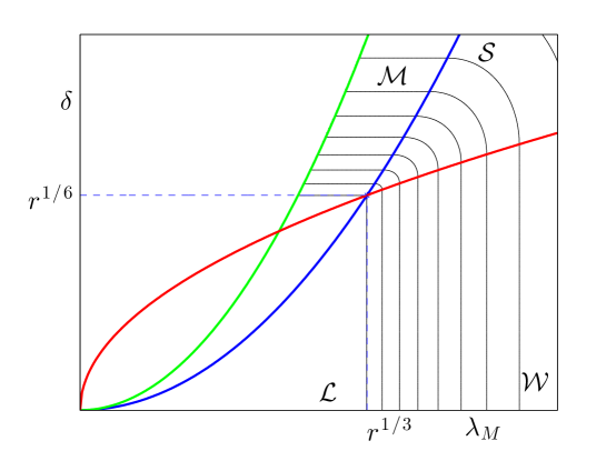
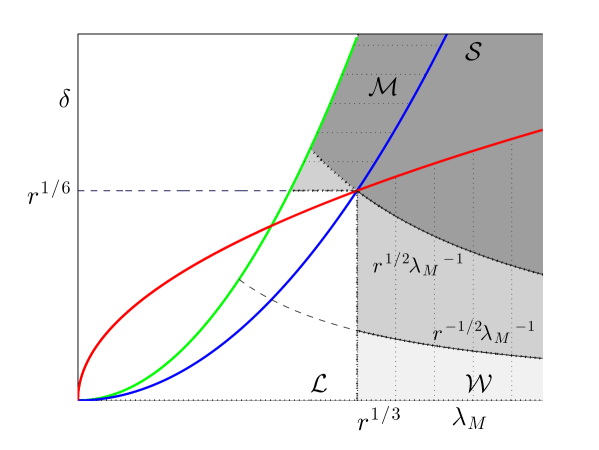
The limit is characterized by an energy per unit area that depends only on the tangential gradient of the deformation. It is obtained from the density of the entropic elasticity by minimizing out the normal component followed by relaxation or quasi-convexification. We compute this by obtaining upper and lower bounds, and provide an explicit formula in Theorem 5.1 (also shown schematically in Figure 1). It is characterized by four regions depending on the in-plane stretch: a solid region where there is no relaxation, a liquid region where wrinkling and microstructure formation drive the effective energy to zero, a wrinkling region where wrinkling relaxes the energy and a microstructure region where stripe domains relaxe the energy. The techniques employed here are in the same spirit as those employed by DeSimone and Dolzmann [14] in three dimensional nematic elastomers.
We also study the oscillations related to the relaxation by characterizing the gradient Young measures associated with the minimizing sequences in Theorem 6.1. We show that the oscillations in the region are necessarily planar oscillations of the nematic director and involve no out of plane deformation while those in the region are characterized by uniform nematic director and wrinkling.
We use the characterization of the gradient Young measure to define the effective state of stress, and show that this coincides with the derivative of the effective or relaxed energy in Theorem 7.1. The Cauchy stress is given in (7.7): it is general biaxial tension in , zero in , uniaxial tension in and equi-biaxial tension in . As described above, the unique attributes of liquid crystal elastomers give rise to this region of equi-biaxial tension compared to membranes of usual elastic materials.
This paper is organized in the following manner: In Section 2, we fix some notation and comment on background results which are used throughout the paper. In Section 3, we describe our model for nematic elastomers, a model which incorporates the entropic elasticity of the polymer matrix and an elastic penalty on the spatial gradient of the director. In Section 4, we derive our effective theory for nematic elastomer membranes based on a notion of -convergence. In Section 5, we provide an explicit formula for the energy density in our effective theory. In Section 6, we characterize the microstructure in the aforementioned regions and . Finally, in Section 7, we conclude with a notion of stress in this effective theory and its physical implications.
2 Preliminaries
We gather here the notation and some background results which we use throughout the paper. We denote with the dimensional Euclidian space endowed with the usual scalar product and norm . The unit sphere in is denoted by and it is defined as the set of all vectors with . The space of matrices with real entries is labeled with . When we denote with the orthogonal group of the matrices for which , where is the identity in and with the rotation group of the matrices with . Letting now , stands for the matrix of all minors of , . In the case , if
If is a smooth map, then is normal to the surface with equation . Letting , , by Proposition 5.66 [11] it follows that
| (2.1) |
Later in this paper we label the norm of , with a matrix, with . Furtheremore, we simply write both when dealing with the adjugate of and matrices.
Finally, we state a version of the polar decomposition theorem: given any and any rectangular Cartesian basis, there exist such that
| (2.2) |
for
| (2.6) |
In fact, are the principle values of .
We now recall some concepts in calculus of variations (cf. [11]). We say that is polyconvex if there exists a convex function which depends on the vector of all the minors of such that . In the case then with . We say that is quasiconvex if, at every , we have
for every . Note that the foregoing inequality holds for every open and bounded subset of with [3]. Finally, is rank-one convex if is a convex function for all with .
If a function is not quasiconvex, we define the quasiconvex envelope of as
Analogously, we define as the convex, polyconvex and rank-one convex envelopes respectively of . In the general case of extended-value functions, convexity implies polyconvexity and polyconvexity implies both rank-one convexity and quasiconvexity, but quasiconvexity alone does not imply rank-one convexity. Therefore, if , we have
| (2.7) |
On the other hand, in the case of a real-valued functions, quasiconvexity implies rank-one convexity and hence, if , we have
| (2.8) |
We give an alternative representation formula for the rank-one convex envelope of a function
with and . Family satisfies a compatibility condition here labelled with and defined in [11, Sec. 5.2.5]. In the same spirit we define semiconvex hulls of a compact set . The set
is the polyconvex hull of . The quasiconvex hull and the rank-one convex hull are defined analogously. The lamination convex hull of is defined
Equivalently, can be defined by succesively adding rank-one segments (see [14]), i.e.
where and
The relations between the different notions of convexity imply the inclusions (see [14])
We refer the interested reader to [11] and [24] for a discussion of all the different notions of convexity and their relations.
Finally, we introduce the notion of a gradient Young measure that characterize the statistics of the fine-scale oscillations in the gradients weakly converging sequences (cf. [24]). We define a homogenous gradient Young measure to be a probability measure that satisfies Jensen’s inequality for every quasiconvex function whose norm can be bounded by a quadratic function. Let denote the space of signed Radon measures on with the finite mass paring
Then the space of homogenous gradient Young measures is given by
| (2.9) |
3 Model of nematic elastomers
Consider a nematic elastomer occupying a region in its reference configuration, and assume that it is in its stress-free isotropic state in this configuration. Let describe the deformation and describe the director field. We denote to be the reference gradient of some field and to be the spatial gradient of . It follows where is the deformation gradient.
We take the Helmholtz free energy density of the nematic elastomer to be the sum of two contributions:
where the describes the entropic elasticity of the underlying polymer chains of the nematic elastomer and describes the elasticity of the nematic mesogens.
Following Bladon, Terentjev and Warner in [6, 33], we take the entropic elasticity to be of the form
| (3.1) |
where
| (3.2) |
is the step-length tensor. Here is the shear modulus of rubber and is the (non-dimensional) backbone anisotropy parameter. Note that for the energy reduces to that of a neo-Hookean material. As most nematic rubbers are nearly incompressible [33], we prescribe to be a finite only for volume-preserving deformations. We can substitute for and write
| (3.3) |
For future use, we define a purely elastic energy by taking the infimum over directors. Following DeSimone and Dolzmann [14],
| (3.4) |
where
| (3.5) |
Here is the largest eigenvalue of . Energy density is not quasiconvex and the quasiconvex envelope has been computed in [14].
Following Oseen, Zocker and Frank, (see for example, [15]), we take the elasticity of the nematic mesogens to be of the form
| (3.6) |
where and are the spatial divergence and curl of the director respectively, and are known as the splay, twist and bend moduli respectively. Notice that this is a non-negative quadratic form in and . It turns out that these moduli are very close to each other and one can introduce an equal modulus approximation
| (3.7) |
where the second equality holds formally. Importantly, from a mathematical point of view, any given of the form (3.6) can be bounded from above and below by equal moduli approximations, and therefore all the results we prove for the equal modulus approximation hold for the more general form. Finally, since we assume incompressibility or , so that
| (3.8) |
Putting these together, the Helmholtz free energy of our nematic elastomer, , is given by
| (3.9) |
where for definiteness, the set of admissible fields is
The ambient space for deformations, , is optimal since for satisfying , satisfies the growth and coercivity
| (3.10) |
independent of . Here depends on and . The ambient space for the director field, , may not be optimal. Nevertheless, consider the following:
Remark 3.1
Fonseca and Gangbo [17] showed the lower-semicontinuity of
in the space
where and such that , (see Theorem 4.1, [17]). The existence of minimizers in follows from this result. However, notice that this is more regularity than we assume. In fact, the existence of minimizers in is not clear. However, this does not affect convergence or the membrane limit.
4 Membrane Theory
In this section, we derive a theory for nematic elastomer membranes whose three dimensional free energy satisfies (3.9).
4.1 Framework
We consider a nematic elastomer membrane of small thickness which has a flat stress-free isotropic reference configuration . We assume is a bounded Lipschitz domain in . Let describe the deformation and describe the director field so that is the Helmholtz free energy in (3.9) now parameterized by the thickness of the membrane in its reference configuration. We assume , and as .
To take the limit as , we follow the theory of -convergence in a topological space endowed with the weak topology. The general theory can be found in [7] and [12]. In order to deal with sequences on a fixed domain, we change variables via
and set . To each deformation and director field , we associate respectively a deformation and director field such that
| (4.1) |
We set , and following the change of variables above observe
| (4.2) |
where with the in-plane gradient. We also use the identity .
Finally, we take our membrane theory to be the -limit as of the functional defined on ,
| (4.3) |
4.2 The Membrane Limit
Theorem 4.1
Let be as in (4.3) with and as . Then in the weak topology of , is equicoercive and -converges to
| (4.4) |
Here
| (4.5) |
for given in (3.4) and is the quasiconvex envelope of ,
Equivalently:
-
(i)
for every sequence such that , there exists a independent of such that up to a subsequence
-
(ii)
for every such that in ,
-
(iii)
for any , there exists a sequence such that in and
The result for the case was provded by Conti and Dolzmann [10] (Theorem 3.1 there).
Theorem 4.2 (Conti and Dolzmann [10])
Remark 4.3
A different dimension reduction theory for hyperelastic incompressible materials was developed by Trabelsi [30],[31] under similar assumptions. Trabelsi shows that the membrane energy density (integrand of ) is given by . From the proof of Theorem 5.1 below, it follows that (and hence ). Thus the two limits agree.
Remark 4.4
We remark on some general properties of the purely elastic portion of our nematic elastomer energy density. in (3.5) is Lipschitz continuous, is non-negative, and there exists a constant such that
| (4.6) |
The energy in (4.5) is given by
| (4.7) |
and satisfies
| (4.8) |
with . The effective energy density is quasiconvex, Lipschitz continuous on bounded sets and its definition does not depend on the choice of the domain , as long as it is open, bounded and . Furthermore, there exists (Lemma 3.1, [10]) a constant such that
| (4.9) |
Proof of Theorem 4.1. Note that trivially,
| (4.10) |
Therefore, the compactness and lower bound (Properties (i) and (ii) in Theorem 4.1) follow from Theorem 4.2. It remains to show Property (iii). This is done in Proposition 4.6.
Before we proceed, we note that the fact that the limit is independent of is similar to the following result of Shu [29]. He also provides some heuristic insight. Since the membrane limit optimizes the energy density over the third column of the deformation gradient, there is little to be gained by oscillations parallel to the thickness. Consequently, penalizing these oscillations with does not affect the limit.
Theorem 4.5 (Shu [29])
Let as , and be continuous and bounded from above and below by respectively for some . Then, in the weak topology of , the functional
converges to
where .
4.3 Construction of Recovery Sequence
It remains to construct a recovery sequence to prove is the -limit to .
Proposition 4.6
For every independent of , there exists a sequence such that in and
| (4.11) |
Our construction also draws heavily from Conti and Dolzmann [10]. The main difference is that we need additional regularity for our recovery sequence . We summarize the Conti-Dolzmann construction in two lemmas. The first lemma regards the construction of a sequence to go from the energy density to on . For our analysis, the important observation is that in the limit the deformation gradient is constant on an increasingly large subset of . The second lemma regards the extension of smooth maps on to incompressible deformations on .
Lemma 4.7 (S. Conti and G. Dolzmann [10])
For any , there exists a sequence such that everywhere, in as , and
| (4.12) |
Moreover, the sequence has the following properties:
-
(i)
for each , is defined on a triangulation of which is the set of at most countably many disjoint open triangle whose union up to a null set is equal to , and is the jump set given by
-
(ii)
there is a sequence of boundary layers such that and as , and the set is defined to be
-
(iii)
if is nonempty, then is a constant on this set and we set
(4.13) -
(iv)
is bounded away from zero in the sense that for some sufficiently small, the inequality
holds everywhere.
Lemma 4.8 (Conti and Dolzmann [10])
Let satisfy
Then there exists an and an extension such that and everywhere. Moreover, for all the pointwise bound
holds, where can depend on and .
We construct a recovery sequence and thereby prove Proposition 4.6 in 4 parts. In Part 1, we take a sequence of smooth maps as in Lemma 4.7 and show that we can construct a sequence of smooth vector fields such that in . In Part 2, we use Lemma 4.8 to extend appropriately to a deformation on , i.e . In Part 3, we construct a sequence of director fields on which enables passage from to . Finally, in Part 4 we show that we can take an appropriate diagonal sequence as which proves Proposition 4.6.
Proof of Proposition 4.6. Let independent of . Then is bounded in (with abuse of notation). By Lemma 4.7, we find a sequence such that everywhere, in , the energy is bounded in the sense of (4.12), and the sequence satisfies properties (i)-(iv) from the lemma.
Part 1. We define the smooth vector field on the triangulation for in Lemma 4.7 (i). On each nonempty there exists a constant defined in Lemma 4.7 (iii), and it is full rank. Then by (4.7), has a minimizer for . Motivated by this observation, we let
| (4.14) |
which via (3.4) implies
| (4.15) |
Consider the vector field,
| (4.16) |
This is well-defined given Lemma 4.7 (iv). Moreover, since is smooth, . Further, since , we have
| (4.17) |
Let be given by
| (4.18) |
Here is a cutoff function which equals 1 at least on the entirety of the subset . Notice when , the determinant constraint is satisfied trivially by (4.17). Conversely, combining (4.15) and (4.17),
since on this set. We then conclude in , and this completes Part 1.
Part 2. Fix . From Part 1 we have satisfying in . Hence, there exists an and a such that the properties of Lemma 4.8 hold replacing with and with . Let and be the restriction of to . Further, let be associated to using (4.1). From Lemma 4.8, we conclude , and
| (4.19) |
Here is a constant depending on and , and the second inequality above follows since . From these properties we conclude as ,
| (4.20) |
This concludes Part 2.
Part 3. As in Part 2, we keep fixed. From Lemma 4.7 (i) we have that (up to a set of zero measure), though this union can be countably infinite. From herein, we choose a finite collection of triangles so that
| (4.21) |
Then for each of the triangles for which the set is nonempty, let
| (4.22) |
Further, let be the piecewise constant function on given by
| (4.23) |
Here is a fixed vector in . Then maps to , but it is not in . To correct this, we employ the approach used by DeSimone in [13] (see Assertion 1).
Observe by construction the range of is finite. Hence, there exists an and a closed ball of radius centered at such that . Then the stereographic projection with the projection point as maps the range of to a bounded subset of . Let be a standard mollifier with as in Lemma 4.7 (ii), and consider the composition
This composition is well-defined since the range of is outside a neighborhood of the projection point . Further, maps to using the definition of the inverse of the stereographic projection. Moreover, is differentiable and its argument is smooth. Hence, .
Let be the restriction of to the closure of . Further, let be the extension of to via for each . As a final remark for this part, observe for and ,
| (4.24) |
since and so is constant on , see (4.23). This completes Part 3.
Part 4. From Parts 1-3, we have for each the functions and parameterized by . It remains to bound the functional appropriately and take the . For the bounding arguments, shall refer to positive constant independent of and which may change from line to line. From (3.1), when is finite, it satisfies a Lipschitz condition
As asserted above, is uniformly bounded for . Then since for every , , and ,
| (4.25) |
Here is the estimate obtained from the Lipschitz condition and an application of Hölder’s inequality,
| (4.26) |
We now focus on the first term in the upper bound (4.3). For and , observe
Then,
| (4.27) |
using our result for and since each integrand is nonnegative.
We bound in (4.3). To obtain this bound notice from (4.16). Further, using the coercivity condition of in (4.6), the definition of in (4.14), and the growth in (4.8),
Following these observations, we notice on the sets , by definition (see Lemma 4.7 (iii)) and therefore,
since is as in (4.18). On the exceptional sets, by definition , and the right side above is still an upper bound to . Hence everywhere in ,
using the growth in (3.10), the bound above and the coercivity in (4.8). This implies the bound
| (4.28) |
where recalling (4.3) and (4.21), the remainder is given by
| (4.29) |
To recap, from (4.3) and (4.28), the entropic part of the energy is bounded above by the estimate
| (4.30) |
It remains to bound the elasticity of the nematic mesogens.
Consider the second term of in (4.2). Our deformations and director fields have sufficient regularity, so
| (4.31) |
Here, we used the identity and the definition . We bound the integrand by a constant independent of . To do this, we first consider the pointwise estimate in (4.19). An application of the reverse triangle inequality on this bound yields for small the pointwise estimate
| (4.32) |
Here is a constant which depends only on and . Then satisfies
and so we can bound from above (4.31),
Applying the bound in (4.3) to this estimate, we conclude as desired
| (4.33) |
Here is a constant depending only on , and .
To complete the proof of Proposition 4.6, it remains to show that in the limit as , the energy is bounded as in (4.11). From (4.30) and (4.33),
| (4.34) |
We now fix and take the limit as . Notice from (4.20), as . This implies for some constant independent of . With these two observations, we conclude as , see (4.26). Further, since as , since is independent of . Collecting these results and combining with (4.34),
Finally, using (4.12), the fact that as (, see Lemma 4.7 (ii), and (4.29)) we conclude
We now choose a diagonal sequence as so that this estimate is satisfied and in . This completes the proof.
5 Effective energy of nematic elastomer membranes
In this section, we provide an explicit formula for the effective energy of nematic elastomer membranes.
5.1 Effective energy
Theorem 5.1
Let as in (3.3). For any , let
| (5.1) |
Then, the effective energy of the nematic membrane is given by
| (5.2) |
Here, are the singular values of (i.e., the eigenvalues of ), and
| (5.3) | |||||
| (5.4) | |||||
| (5.5) | |||||
| (5.6) |
Remark 5.2
Some care needs to be taken when dealing with extended real-valued quasiconvex functions. Indeed, the fact that a function is quasiconvex (according to the defintion of Section 2 of this paper) does not imply that the associated functional is sequentially weak∗ lower semicontinuous on [3]. In the current situation, thanks to Remark 4.4, the relaxed energy density has polynomial growth and therefore weak lower semincontinuity is true for the relaxed functional. Alternatively, we refer the interested readers to Ball and James [1] where a more restrictive definition of quasiconvexity for extended real value functions is presented. This definition guarantees weak lower semicontinuity of functionals associated to extended real value integrand functions. It is an easy computation to show that both the approach pursued in what follows and the relaxation technique based on the alternative definition of quasiconvex envelope give the same results for the functionals considered in this paper.
Proof of Theorem 5.1. Recall that the quasiconvex envelope of an extended value function is not in general bounded from above by the rank-one convex envelope. However, we show that this bound is true for . By Remark 4.4, is a finite-valued, a quasiconvex function and . Therefore, if we substitute in we obtain
| (5.7) |
Then, by we conclude
| (5.8) |
and recover the classical inequality
| (5.9) |
We show in Lemma 5.3 and Lemma 5.4 that . We show in Lemma 5.5 that . Combining these with (5.9),
| (5.10) |
and the result follows.
5.2 Step 1: A formula for
Proof. The proof is an explicit calculation. To begin, if , then for every . This implies for every . Then . Thus for the remainder of this section, we restrict our attention to the case that .
Let and . Then, is equivalent to the optimization
Here is a convex, differentiable function and is an affine equality constraint. It follows that is a global minimizer of this optimization if and only if there exists a such that (see for instance [8], Section 5.5.3). Solving this equation, we obtain
for defined in (3.2).
Let . Since is a global minimizer for the constrained optimization above, . Then from (5.1), it follows that . For this optimization, we simplify the analysis through a change of variables. We write for , and a diagonal matrix as in (2.2) with as the singular values. We can say since . Additionally, we set , and impose the constraint via . Then by direct substitution,
where
Here since . Further, we let , and set
| (5.16) |
Note that the constraint implies .
is dependent on only four constrained variables. Consider the closed set
combined with the constraint give the admissible set for . Hence, we have
Observe that
by (5.2) since the second term in the brackets is non-positive. Then,
where
is a continuous function on this constrained set (which is moreover bounded in ). It is also differentiable for in the open domain . It follows that the infimum is attained. Further, minimizes only if it is on the boundary, i.e or , or it is a critical point, i.e. and .
We proceed case by case. Letting , observe in (5.13). For the other boundary , we obtain in (5.14). Finally, in computing the critical point , we obtain
Direct substitution yields the equation given for the finite portion of in (5.15). Recalling that must lie in the domain , we set if does not lie in this set. This is the full result in (5.11).
5.3 Step 2: Upper bound or
Proof. We prove this in two parts. In Part 1, we prove that is polyconvex and in Part 2 we prove that . The result follows.
Part 1. We now show that is polyconvex. First, observe from (5.2) that there exists a function (here by we denote the set of all non-negative real numbers) such that
| (5.18) |
It also follows by verification (also see Proposition 2 of DeSimone and Dolzmann [14]) that is convex and is non-decreasing in each argument (i.e., in nondecreasing in for fixed and nondecreasing in for fixed . We then notice that is convex in . Further, is convex in . Since the composition of convex function with a non-decreasing and convex function results in a convex function, we conclude that there exists a convex function such that
Combining with (5.18), we conclude that
| (5.19) |
for convex . By definition of polyconvexity, is polyconvex.
Part 2. We now show that . We show by explicit calculation in the Appendix A that
It follows that
from (5.11).
5.4 Step 3: Lower bound or
The proof makes repeated use of lamination. We collect the calculations in the following proposition.
Proposition 5.6
Let with , and define
Then, for and for .
Proof. We begin with . Let with . Using the polar decomposition theorem, we can take
Define
Note that , since , rank and . Therefore, .
The proof of is similar (also see [14, Theorem 3.1]). Again, using the polar decomposition theorem, we can take as a diagonal matrix. First, let us assume and which corresponds to and define
| (5.24) |
Note . Further, the eigenvalues of are
So the choice
makes . Therefore, . Further, and rank . For the case such that , replace the diagonal entries in (5.24) with and repeat the argument. Therefore, .
Proof of Lemma 5.5. We show that
| (5.25) |
region by region. In the region , note and the result follows.
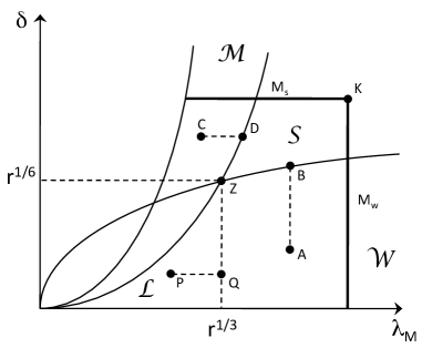
Now, let with and . This corresponds to the point in Figure 2. Let
This set corresponds to the point in Figure 2a. By Proposition 5.6, we have . Therefore, there exists and with such that
Above, the first two inequalities follow from the fact is rank-one convex and . The following two equalities is by explicit verification of the formula.
Now, let with and . This corresponds to the point in Figure 2a. Let
This set corresponds to the point in Figure 2a. Therefore, by Proposition 5.6, we have . Therefore, arguing as before, .
Finally, let with and . This corresponds to the point in Figure 2a. Let
and
These sets correspond to the points and in Figure 2-(a) respectively. From Proposition 5.6, . Further, again by Proposition 5.6, . In other words, . We can again argue as above to show that as required.
6 Characterization of fine-scale features
The energy density is not quasiconvex. Thus a membrane with this energy density is able to relax its energy to that of through the introduction of fine-scale features. In this section, we characterize these features. Briefly, we show that the features in region are essentially planar involving oscillations of the director (i.e., no wrinkling) while those in are necessarily wrinkles (i.e., uniform director). Further, we show that there are no fine-scale features in region .
To characterize the fine-scale features, we consider the two-dimensional energy
| (6.1) |
subject to affine boundary conditions, i.e the space of deformations with . It is known (cf. Lemma 3.1(ii) and Lemma 6.2, [10]) that there exists weakly converging minimizing sequences that satisfy
| (6.2) |
Let be any gradient Young measure generated by such a sequence. Since is a minimizing sequence for , it is also a minimizing sequence for the relaxation . Further, since is non-negative and bounded as in (4.9), it follows from Theorem 1.3 of Kinderlehrer and Pedregal [20] that
| (6.3) |
and for every measurable whenever the sequence converges. As an immediate consequence, we obtain the identities
| (6.4) |
Now, since is a normal integrand, the fundamental theorem of Young measures gives an inequality, (cf. Definition 6.27 and Theorem 8.6, [18]). Thus,
where we use the fact that . It follows . Again using the fact that and (6.4) we conclude
| (6.5) |
By the localizing properties of gradient Young measures (cf. Theorem 2.3 of [19]), we conclude that the fine-scale features which arise from minimizing sequences of are described by the homogenous gradient Young measures which admit the identities,
| (6.6) |
We present a characterization of this in the following theorem.
Theorem 6.1
Let , and let
| (6.7) |
be the set of homogenous gradient Young measures that satisfy (6.6). Then, there exists . Further the following is true.
-
1.
(The region ) Suppose . Set . Let the singular value decomposition (cf. (2.2)) of be given by with .
If , then
(6.8) where is orthogonal to the plane of the reference configuration of the membrane and
(6.12) -
2.
(The region ) Suppose . Set . Further, set and to be the unique pair (up to a change in sign) of vectors which satisfy .
If , then
-
3.
(The region ) Suppose .
If , then
-
4.
(The region ) Suppose . If , then is a Dirac mass. So .
Theorem 6.1 has striking physical implications. First consider Part 1 corresponding to region and consider the particular case when . Consider any and its characterization in (6.8). Since , it follows for each . In other words, maps to . Thus, all the oscillations are in the plane. Further, for such matrices ,
for and . The first of these identities follows from the fact that (see Lemma 6.2 below) and Lemma 5.3, while the second follows from the fact that the largest principal value of is . Importantly, the director is always in the plane. In summary, the director oscillates in the plane and oscillations create no out of plane deformation. The case is similar except the plane is oriented by the rotation . Thus, the fine-scale features in is limited to in-plane oscillations of the director.
Now consider Part 2. First consider the case when . Using an argument as before, for any ,
for , and . In other words, the director is fixed with an in-plane direction . Further, notice is necessarily of the form
in the frame for that satisfies . In other words, the membrane is uniformly deformed and the fine features are related to rotations about a fixed axis . In other words, oscillations represent wrinkling and these oscillations are always perpendicular to . The general case is similar except a uniform rotation orients to .
Part 3 says that region involves only the spontaneously deformed states while Part 4 says that there are no fine-scale features in .
We now turn to the proofs of the theorems. They rely on the following lemmas.
Proof of Lemma 6.2. Recall from Section 5 that we may write and where respectively for . Recall also that is a convex, and it is non-decreasing in each argument. Also, . Finally, are quasiconvex functions bounded quadratically. Therefore, for every homogenous gradient Young measure with ,
| (6.15) |
Here, the first inequality follows from the Jensen’s inequality satisfied by homogenous gradient Young measures since are quasiconvex with the appropriate growth and is non-decreasing in each argument. The second inequality follows from the convexity of , and the third follows since .
Now, for any , each inequality in (6) is an equality. This restricts the support of . To deduce this restriction, suppose that the point corresponds to point C in Figure 2(a).
Consider the first inequality. By quasiconvexity and growth conditions, and . In the space in Figure 2(a), these inequalities imply the point cannot be to the left or below point C. Further, every point to the right and above the point C has higher (cf. Figure 1) except the line between and including the points C and D. Hence,
| (6.16) |
Next, consider the last inequality. Since only on (see Figure 2b), we conclude
| (6.17) |
It remains to consider the middle inequality in (6). We do this in Proposition 6.4 below. If the middle inequality is an equality, we show in the proposition the support of satisfies (6.13). This completes the proof.
Proposition 6.4
Proof. Set and
If , then by the polyconvexity of , contradicting (6.16). Now consider the case . Set
Clearly, and
| (6.19) |
From the equality in (6), . Further, notice from the convexity of that
| (6.20) | ||||
| (6.21) |
Now, in the space shown in Figure 2(a), the definitions above imply that the point is a point above the line CD while is below the line CD such that the line joining these points intersect CD. It is easy to verify by explicitly computing the derivative along such lines (or by inspecting Figure 1), that is strictly convex in such segments. Therefore,
| (6.22) | ||||
The last inequality follows from (6.20). However, this contradicts the assumption (6.18).
Finally, given (6.23) and since (see 6.16), it follows that . But this is just a single point in the space, and it’s given by (6.13). Thus, we conclude the proposition.
The proof of Lemma 6.3 is very similar and omitted.
Part 1. For any with and for any , the support of satisfies (6.13) by Lemma 6.2. Note that is equivalent to stating that the principal values of are and . Therefore, by the singular value decomposition theorem (2.2), it follows that
| (6.24) |
for is given in (6.12).
Now, for any , it is an easy calculation to find that . Further for of the form (2.6), . Further, the adjugate is a minor and therefore . Recalling the support (6.24) of , we conclude
Note that , and for each . In other words, the equation above states that an average of a distribution on yields an element of . However, since each element of is an extreme point, it means that the distribution is concentrated at a single point on . That is, if we let , then . The result follows.
Part 2. For any with and for any , it follows from the definition of that
| (6.25) |
So,
However, from Lemma 6.3, we see that for each . Therefore, for each . We conclude that for each . Setting for and substituting in (6.25), we conclude that for for each . The result follows.
Part 3. For any with , the result follows from the fact that is non-negative and if and only if .
Part 4. Finally, let such that , . Recall and is strictly convex in . Thus,
This is actually equivalent to the set (6.26) given in Proposition 6.5 below since . The result follows from the proposition.
Proposition 6.5
Let such that the singular values satisfy the strict inequality
Suppose is a probability measure on the space of matrices such that and
| (6.26) |
Then (up to a set of measure zero) is a Dirac mass at .
Proof. To begin, set . We let and be sets of orthonormal vectors such that
| (6.27) |
Let . This is a convex function. Therefore, by Jensen’s inequality and given with satisfying (6.27),
| (6.28) |
Conversley, applying a similar change of variables (6.27) to the , we see
since by assumption . Here, denotes the direction cosine between and . Combining this observation with (6.28), we deduce (up to a set of measure zero), . This implies (up to a change in sign) in measure. Since and are orthogonal, it follows that (up to a change in sign) in measure.
We repeat this argument substituting with the convex function . It follows that (up to a change in sign) and in measure. The fact that ensures the eigenvectors are fixed and not oscillating in sign with some non-zero measure. The conclusion follows.
7 State of stress and connection to tension field theory
In this section, we seek to understand the state of stress in the membrane.
Formally, consider an incompressible energy density of the form in (3.4) and assume is differentiable. The Piola-Kirchhoff and the Cauchy stress are defined as
| (7.1) |
where is the indeterminate pressure (Lagrange multiplier to enforce incompressibility) and is identity. We find by requiring the tractions to be zero on faces of the membrane. Alternately, recall that we obtain the membrane energy density by writing and minimizing with (when is full rank). The minimizer satisfies
| (7.2) |
Above, denotes derivative with respect to the third column of the deformation gradient. Substituting this back in (7.1) and writing we obtain a characterization of the state of stress in the membrane.
| (7.3) |
Notice that these depend only on .
However, the effective energy of the membrane is not but its relaxation. In other words, energy minimization with the integral of can lead to fine-scale oscillations, and thus the stress may also oscillate on a fine scale. Therefore, we need to understand the overall of effective stress. Ball et al. [2] have shown that if is differentiable and satisfies certain growth conditions, then is a function. Moreover, can be written in terms of and a homogeneous gradient Young measure generated by minimizing sequences of , i.e.
| (7.4) |
Unfortunately is an extended function (equal to when ), and the analogous result is unknown. However, our resulting effective energy is finite everywhere and is differentiable except on a boundary. So have the following characterization of the stress.
Theorem 7.1
Let , let be the open set , and let such that . If is a homogenous gradient Young measure generated by minimizing sequences for the energy in the space (see (6.1)) with support in , then
| (7.5) | |||
| (7.6) |
Further, the Cauchy stress has the following explicit characterization.
| (7.7) |
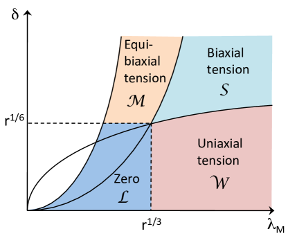
Before we prove the theorem, we make a few comments on the physical implications. First, the membrane is always in a state of plane stress in the tangent plane. Second, the principal stresses (the eigenvalues) are always non-negative. Therefore, the membrane can not sustain compressive stress. Further, the stress is zero in region , uniaxial tension in , equi-biaxial tension in and biaxial tension in . The different regimes are shown in Figure 3.
To understand this further, consider the special case when this theory reduces to that of neo-Hookean elastic membrane. The region now disappears and we are left with regions and with zero, uniaxial tension and biaxial tension respectively as in the traditional tension field theory [25, 26, 28].
Nematic elastomers membranes with are characterized by an additional region where the state of stress is equi-biaxial tension. This is true even though, the principal stretches can be unequal. In other words, one can have shear strain but no shear stress. This is a potentially useful attribute of liquid crystal elastomers in membrane applications.
We turn now to the proof of Theorem 7.1.
Proof of Theorem 7.1. Recall from Section 5 that we may write and . Now, any has the representation
| (7.8) |
where and are orthonormal and are the singular values of . These singular values (and therefore ) are continuously differentiable with respect to as long as they are distinct, i.e. with
(cf. Corollary 3.5 and Theorem 5.1, [27]). We can use this fact and the representation for in Theorem 5.1 and Lemma 5.3 to conclude that and are continuously differentiable on .
The rest of the proof is by computation and verification.
Case 1: . Set . According to Theorem 6.1 Part 1, . We can now apply the representation (7.8) to and to write the identity as
| (7.9) |
Another implication of Theorem 6.1 is any can be written as where arises from the identity , for some and such that . Here, is orthogonal to the reference configuration of the membrane. Without loss of generality, we assume . Now for each there is a corresponding such that . In other words, the vectors and span the plane perpendicular to for each . Moreover , and therefore and also span this plane. Now, let be a degree rotation about and be a degree rotation about so that and . Since span the same plane as , and the same plane as , we have the following relation. If , then
| (7.10) |
If , then
| (7.11) |
Thus, pre-multiplying and post-multiplying the identity in (7.9) by and respectively yields the identity
| (7.12) |
It is easy to verify . Thus, combining explicit differentiation evaluated in with the identity (7), we observe
| (7.13) |
Finally, it can be verified explicitly that coincides with (7). This gives the identity (7.5) for region .
Similarly,
| (7.14) |
The fourth equality uses the fact that the basis always spans the same plane. Finally, it can be verified explicitly that coincides with (7) in this region. This gives the identities (7.6) and (7.7) for region .
Case 2: . Set . Following Theorem 6.1 Part 2, and so any satisfies . In addition, for the vectors and such that , also satisfies . Writing as in (7.8), we observe using the properties of the set ,
| (7.15) |
Here, denotes the direction cosine from to . Applying the squared norm to the identities in (7) yields . Since in , we deduce from this equation that . That is, is up to a change in sign equal to . Substituting for back into (7), we find when , or alternatively
| (7.16) |
Now, it is easy to verify explicitly . Thus, combining explicit differentiation evaluated in with (7.16),
| (7.17) |
Finally, it can be verified explicitly that coincides with (7). Therefore, the identity (7.5) is satisfied for .
Similarly,
| (7.18) |
For the last equality, recall for . Finally, it is easy to verify explicitly that coincides with (7) in this region. Thus, we have the identities (7.6) and (7.7) for region .
Case 3: . According to Theorem 6.1 Part 3, . We see that on and similarly on . The identities (7.5), (7.6) and (7.7) for region .
Case 4: . According to Theorem 6.1 Part 4, is a Dirac mass. According to Theorem 5.1, and coincide on . The identities (7.5), (7.6) and (7.7) for region .
Acknowledgments
This work was partially conducted when PC held a position at the California Institute of Technology. We acknowledge support from the US Department of Energy National Nuclear Security Administration (Award Number DE-FC52-08NA28613, all authors), the US National Science Foundation (Award Number OISE-0967140, PPP and KB) and the European Research Council under the European Union’s Seventh Framework Programme (FP7/2007-2013, ERC grant agreement N. 291053, PC). The authors thank Jan Kristensen for his advice on a draft version of the paper.
Appendix A Appendix A: Proof of Part 2 of Lemma 5.4
A.1
First, in the region of liquid behavior there is nothing to prove. Therefore, referring to Fig. 4, we are left with showing that in the light gray region of equations for . Recalling that in this region , it is enough to prove that
| (A.1) |
The critical point of is attained at . This corresponds to a minimum, yielding the following inequality
| (A.2) |
which is indeed true for . Then, evaluation of along the curve does not improve the inequality above.
A.2
We focus on the interval corresponding (if again we ignore the region ) to the dark gray area in Fig. 4. This set has a non-empty intersection with both the simple-laminate regions , and the regime of solid behavior . First of all, notice that if then and there is nothing to prove.
Let us assume , . This corresponds to a subset of for which we have . We are left with the inequality
which is trivially true.
Then, let us assume . This is a subset of the region for which we have . The inequality
follows trivially.
A.3
We now focus on the interval corresponding to the silver/intermediate gray area in Fig. 4. Notice that if we remove the region (for which there is nothing to prove), we are left with two disjoint subsets.
We begin with considering . Since in this region , it is enough to show that
which is equivalent to
| (A.3) |
The critical point of is attained at . Then, we have to evaluate on the curves of equations and . Notice that, for we have that while for we have and from discussion of these cases in Paragraph A.2 and A.1, respectively, it therefore follows that is true.
To conclude, we have to prove that the inequality holds in the remaining subregion defined by , and . This subset is contained in the region in which case we have . Therefore, we are left with proving the inequality
equivalent to
| (A.4) |
In order to prove the inequality above it is enough to evaluate the function on the boundary of the region defined on the right hand side of . This yields the following two relations
| (A.5) |
| (A.6) |
obtained by evaluating for and respectively. To show that holds it is convenient to operate the change of variable and thus writing as follows
| (A.7) |
which can be easily shown to be true . Then, it is immediate to prove .
References
- [1] J. Ball, R.D. James, Incompatible sets of gradients and metastability, to appear on the Archive for Rational Mechanics and Analysis
- [2] J. Ball, B. Kirchheim, J. Kristensen, Regularity of quasiconvex envelopes, Calc. Var. 11, 333-359 (2000)
- [3] J. Ball, F. Murat, -Quasiconvexity and variational problems for multiple integrals. J. of Funct. Analysis 58, 225-253 (1984)
- [4] M. Barchiesi and A. DeSimone, Frank energy for nematic elastomers: A nonlinear model, ESAIM: COCV 21, N. 2 372-377 (2015)
- [5] K. Bhattacharya and R.D. James, A theory of thin films of martensitic materials with applications to microactuators, J. Mech. Phys. Solids 47, 531-576 (1999)
- [6] P. Bladon, E. M. Terentjev, M. Warner, Transitions and instabilities in liquid-crystal elastomers, Phys. Rev. E 47, R3838-R3840 (1993)
- [7] A. Braides, -convergence for beginners, Oxford University Press (2002)
- [8] S. Boyd and L. Vandenberghe, Convex optimization, Cambridge University Press (2004)
- [9] S. Conti, A. DeSimone, G. Dolzmann, Soft elastic response of stretched sheets of nematic elastomers: a numerical study, J. Mech. Phys. Solids 50, 1431-1451 (2002)
- [10] S. Conti and G. Dolzmann, Derivation of elastic theories for thin sheets and the constraint of incompressibility, Analysis, modeling and simulation of multiscale problems, 225-246 Springer (2006)
- [11] B. Dacorogna, Direct methods in the calculus of variations, 2nd ed. Springer, New York (2008)
- [12] G. Del Maso, An introduction to -convergence, Birkhäuser, Boston (1993)
- [13] A. DeSimone, Energy minimizer for large ferromagnetic bodies, Arch. Rat. Mech. Anal. 125, 99-143 (1993)
- [14] A. DeSimone, G. Dolzmann, Macroscopic response of nematic elastomers via relaxation of a class of -invariant energies, Arch. Rat. Mech. Anal. 161, 181-204 (2002)
- [15] P.G. de Gennes and J. Prost, The physics of liquid crystals, Oxford University Press (1993)
- [16] F.C. Frank, I. Liquid crystals. On the theory of liquid crystals, Faraday Soc. 25, 19-28 (1958)
- [17] I. Fonseca, W. Gangbo, Local invertibility of sobolev functions, SIAM J. Math. Anal. 26(2), 280-304 (1995)
- [18] I. Fonseca, G. Leoni, Modern methods in the calculus of variations: spaces, Springer Monographs in Mathematics (2007)
- [19] D. Kinderlehrer, P. Pedregal, Characterizations of Young Measures Generated by Gradients, Arch. Rat. Mech. Anal. 115, 329-365 (1991)
- [20] D. Kinderlehrer, P. Pedregal, Weak convergence of integrands and the Young measure representation, SIAM J. Math. Anal. 23(1), 1-19 (1992)
- [21] I. Kundler and H. Finkelmann, Strain-induced director reorientation in nematic liquid single crystal elatomers, Macromol. Chem. Rap. Comm. 16, 679-686 (1995)
- [22] P.D. Olmsted, Rotational invariance and Goldstone modes in nematic elastomers and gels, J. de Phy. II. 4, 2215-2230 (1994)
- [23] H. Le Dret and A. Raoult, The nonlinear membrane model as variational limit of nonlinear three-dimensional elasticity, J. Math Pures Appl. 74, 549-578 (1995)
- [24] S. Müller, 1999. Variational methods for microstructure and phase transitions, in: Proc. C.I.M.E. summer school “Calculus of variation and geometric evolution problems”, Cetraro 1996, (F. Bethuel, G. Huisken, S. Müller, K. Steffen, S. Hildebrandt, M. Strüwe eds.), Springer LNM vol. 1713.
- [25] E.H. Mansfield, Load transfer via a wrinkled membrane, Proc. Royal Soc. Lond A 316, 269-289 (1970)
- [26] A.C. Pipkin, The relaxed energy density for isotropic elastic membranes, IMA J. Appl. Math. 36, 85-99 (1986)
- [27] L. Qi, R.S. Wormersley, On extreme singular values of matrix valued functions, J. Convex Anal. 3, 153-166 (1996)
- [28] D.J. Steigmann, A.C. Pipkin, Finite Deformations of wrinkled membranes, Q.J. Mech. Appl. Math. 42, 427-440 (1989)
- [29] Y.C. Shu, Heterogeneous thin films of martensitic materials, Arch. Rational Mech. Anal. 153, 39-90 (2000)
- [30] K. Trabelsi, Incompressible nonlinearly elastic thin membranes, C. R. Acad. Sci. Paris, Ser. I 340, 75-80 (2005)
- [31] K. Trabelsi, Modeling of a membrane for nonlinearly elastic incompressible via Gamma-convergence, Analysis and Appl. 4 N.1, 31-60 (2006)
- [32] M. Warner, P. Bladon, and E.M. Terentjev ,“Soft elasticity” - deformation without resistance in liquid crystal elastomers, J. de Phys. II 4, 93-102 (1994)
- [33] M. Warner, E.M. Terentjev, Liquid crystal elastomers, Oxford Science Publ. (2003)
- [34] B. Yan, An explicit formula of reduced membrane energy for incompressible p-Dirichlet energy, Appl. Analysis 88 N.9, 1321-1327 (2009)