Analytic Photometric Redshift Estimator for Type Ia Supernovae
From the Large Synoptic Survey Telescope

Abstract

Accurate and precise photometric redshifts (photo-z’s) of Type Ia supernovae (SNe Ia) can enable the use of SNe Ia, measured only with photometry, to probe cosmology. This dramatically increases the science return of supernova surveys planned for the Large Synoptic Survey Telescope (LSST). In this paper we describe a significantly improved version of the simple analytic photo-z estimator proposed by Wang (2007) and further developed by Wang, Narayan, and Wood-Vasey (2007). We apply it to 55,422 simulated SNe Ia generated using the SNANA package with the LSST filters. We find that the estimated errors on the photo-z’s, $\sigma_{z_{\rm phot}}/(1+z_{\rm phot})$, can be used as filters to produce a set of photo-z’s that have high precision, accuracy, and purity. Using SN Ia colors as well as SN Ia peak magnitude in the $i$ band, we obtain a set of photo-z’s with 2 percent accuracy (with $\sigma(z_{\rm phot}-z_{\rm spec})/(1+z_{\rm spec})=0.02$), a bias in $z_{\rm phot}$ (the mean of $z_{\rm phot}-z_{\rm spec}$) of $-9\times 10^{-5}$, and an outlier fraction (with $\left|(z_{\rm phot}-z_{\rm spec})/(1+z_{\rm spec})\right|>0.1$) of 0.23 percent, with the requirement that $\sigma_{z_{\rm phot}}/(1+z_{\rm phot})<0.01$. Using the SN Ia colors only, we obtain a set of photo-z’s with similar quality by requiring that $\sigma_{z_{\rm phot}}/(1+z_{\rm phot})<0.007$; this leads to a set of photo-z’s with 2 percent accuracy, a bias in $z_{\rm phot}$ of $5.9\times 10^{-4}$, and an outlier fraction of 0.32 percent.

1 Introduction

The use of Type Ia supernovae (SNe Ia) as cosmological standard candles is a corner stone of modern cosmology, and led to the observational discovery of cosmic acceleration (Riess et al., 1998; Perlmutter et al., 1999). The true nature of cosmic acceleration, dubbed “dark energy” for convenience, remains shrouded in mystery. We do not even know if it is an unknown form of energy (hence appropriately named “dark energy”), or a consequence of the modification of Einstein’s theory of general relativity (“modified gravity”). Probing the true nature of cosmic acceleration requires the measurement of both cosmic expansion history and the growth history of large scale structure (Knox, Song, & Tyson, 2006; Guzzo et al., 2008; Wang, 2008). The use of SNe Ia remains one of the most important methods for measuring cosmic expansion history.

We can expect a dramatic increase in the number of SNe Ia that can be used to measure cosmic expansion history in the coming years and decades. Thousands of SNe Ia are expected from the Dark Energy Survey (DES) (Bernstein et al., 2012), and hundreds of thousands of SNe Ia are expected from Large Synoptic Survey Telescope (LSST) (Abell et al., 2009).

The majority of the SNe Ia from LSST will only have photometry, and will not have spectroscopic redshifts, due to the expensive resources required to obtain follow-up spectroscopy. Fortunately, the redshifts of the SNe Ia can be estimated using multi-band photometry (these approximate redshifts are called photometric redshifts, or photo-z’s). However, the observed photometric SNe need to be classified first using photometry (see “Supernova Photometric Classification Challenge” by Kessler et al. (2010b) for a detailed discussion). Even applying an optimized version of the top performing method from the Supernova Photometric Classification Challenge, the photometric-classification algorithm of Sako et al. (2011) result in over 25% of the resultant photometric SN Ia sample remaining non-Ia SNe (Campbell et al., 2013). We will defer the difficult task of photometric classificationo future work, and focus on the relatively easier task of estimating redshifts of known SNe Ia using photometry only.

SNe Ia with sufficiently accurate and precise photo-z’s can be used for probing cosmology. This would dramatically increase the science return of supernova surveys planned for LSST. Accurate photo-z’s can also enhance the ability of observers to accurately target high redshift SNe Ia for spectroscopy, allowing flexibility and optimization in survey design for Stage III and Stage IV dark energy projects (Albrecht et al., 2006).

In this paper, we build on the previous work by Wang (2007) and Wang, Narayan, & Wood-Vasey (2007), and present a simple analytic photo-z estimator. We apply this photo-z estimator to 55,422 simulated SNe Ia generated using the SNANA package (Kessler et al., 2009b) with the LSST filters. We present our method in Sec.2, describe the simulation of LSST SNe Ia in Sec.3, show our results in Sec.4, and discuss our findings in Sec.5.

2 The Method

The analytic photo-$z$ estimator for SNe Ia proposed by Wang (2007) is empirical, model independent (no templates used), and uses observables that reflect the properties of SNe Ia as calibrated standard candles. It was developed using the SN Ia data released by the Supernova Legacy Survey (Astier et al., 2006).

This method requires a training set of SNe Ia with spectroscopic redshifts. The SNe Ia in the training set are the same as the data, but with known redshifts. The training set is randomly chosen from the data to span the ranges of the colors and magnitudes of the entire data set. This mimics what should be done in practice when real data become available: choose a training set from the data to carry out spectroscopic redshift measurements.

2.1 The Prototype Photo-z Estimator

The prototype photo-z estimator we use here was developed in Wang (2007) and Wang, Narayan, and Wood-Vasey (2007). This estimator uses the fluxes in $griz$ (or $riz$) at the epoch of $i$ maximum flux to make an effective K-correction to the $i$ flux. The first estimate of redshift is given by

$$z_{\rm phot}^{0}=c_{1}+c_{2}g_{f}+c_{3}r_{f}+c_{4}i_{f}+c_{5}z_{f}+c_{6}i_{f}^{2}+c_{7}i_{f}^{3}$$ (1)

where $g_{f}=2.5\log(f_{g})$, $r_{f}=2.5\log(f_{r})$, $i_{f}=2.5\log(f_{i})$, and $z_{f}=2.5\log(f_{z})$, and $f_{g}$, $f_{r}$, $f_{i}$, $f_{z}$ are fluxes in counts, normalized to some fiducial zeropoint, in $griz$ at the epoch of $i$ maximum flux.

Next, the photo-z estimator calibrates each SN Ia in its estimated rest-frame using

$$\Delta i_{15}=2.5\log(f_{i}^{15d}/f_{i}),$$ (2)

where $f_{i}^{15d}$ is the $i$ band flux at 15 days after the $i$ flux maximum in the estimated rest-frame, corresponding to the epoch of $\Delta t^{15d}=15(1+z_{\rm phot}^{0})$ days after the epoch of $i$ flux maximum.

The final estimate for the photometric redshift is given by

$$z_{\rm phot}=\sum_{i=1}^{8}c_{i}\,p_{i},$$ (3)

where the data vector ${\mbox{\bf p}}=\{1,g_{f},r_{f},i_{f},z_{f},i_{f}^{2},i_{f}^{3},\Delta i_{15}\}$. The coefficients $c_{i}$ (i=1,2,…,8) are found by using a training set of SNe Ia with $griz$ (or $riz$, for which $c_{2}=0$) lightcurves and measured spectroscopic redshifts. The jackknife technique (Lupton, 1993) is used to estimate the mean and the covariance matrix of $c_{i}$.

2.2 Photo-z Estimator Applied to LSST Filters

For application to SNe Ia from LSST with photometry only, we have simplified and modified the analytic photo-z estimator for easier application and better performance as follows:
(1) Instead of using the fluxes in all filters except i at the epoch of $i$ maximum flux to make an effective K-correction to the $i$ flux, we just use the peak magnitudes in all filters for each SN to construct an indicator of the spectral shape of the SN.
(2) We add 2nd order terms in the colors for improved accuracy and precision of the estimator.
(3) We replace $\Delta i_{15}$ with $\Delta i_{12}=2.5\log(f_{i}^{12d}/f_{i})$, to increase the sample size, where where $f_{i}^{12d}$ is the $i$ band flux at 12 days after the $i$ flux maximum in the estimated rest-frame, corresponding to the epoch of $\Delta t^{12d}=12(1+z_{\rm phot}^{0})$ days after the epoch of $i$ flux maximum.

Note that our use of $\Delta i_{15}$ was first introduced by Wang (2007) to reduce the scatter in the estimated SN Ia photometric redshifts; it is analogous to the use of $\Delta m_{15}$ in SN Ia calibration, but the use of $i$ band magnitude allows us to include a larger set of SNe Ia in our analysis (Wang, 2007).

The key to obtaining a set of reliable photo-z’s for SNe is to exclude the SNe that are inferred to have unreliable photo-z estimates based on the photometry data alone. We make a first cut in SNe to be used as follows:
(1) Exclude the few SNe that have no $i$-band photometry. This is necessary since we use the $i$ magnitude at maximum light in estimating the photo-z’s.
(2) Exclude SNe that have measured flux uncertainties at maximum light in any passband that exceeds 0.2 magnitude. This is useful in reducing the number of outliers with $\left|(z_{\rm phot}-z_{\rm spec})/(1+z_{\rm spec})\right|>0.1$.
(3) Exclude SNe that do not have $i$-band lightcurve data that extends to 12 days after maximum light in the estimated SN restframe. This enables the refinement of the photo-z estimated using the fluxes at maximum light alone.

We then apply the photo-z estimator as follows:
(1) Divide the SNe according to the passbands in which the SN magnitudes at maximum light are available.
(2) For each set of SNe with photometry in the same passbands, construct the initial photo-z estimate given by

$$z_{\rm phot}^{0} = c_{1}+\sum_{j=1}^{n-1}c_{j+1}(m_{p,j}-m_{p,j+1})$$ (4)

$$+\sum_{j=1}^{n-1}c_{n+j}(m_{p,j}-m_{p,j+1})^{2}$$

$$+c_{2n}i_{p}+c_{2n+1}{i_{p}}^{2}+c_{2n+2}{i_{p}}^{3}$$

where $m_{p,j}$ is the magnitude at maximum light in the j-th passband, $i_{p}$ is the magnitude at maximum light in the $i$ band, $n$ is the number of filters or passbands with available photometry, and $\{c_{j}\}$, $j=1,2,...,2n+2$, are the coefficients to be estimated from using the training set of SNe with spectroscopic redshifts.
(3) Next, calibrate each SN Ia in its estimated rest-frame using

$$\Delta i_{12}=i_{12d}-i_{p}$$ (5)

where $i_{12d}$ is the $i$ band magnitude at 12 days after the $i$ maximum light in the estimated rest-frame, corresponding to the epoch of $\Delta t^{12d}=12(1+z_{\rm phot}^{0})$ days after the epoch of $i$ maximuml light.

The final estimate for the photometric redshift is given by

$$z_{\rm phot}=\sum_{j=1}^{2n+3}c_{j}\,p_{j},$$ (6)

where the data vector ${\mbox{\bf p}}=\{1,(m_{p,1}-m_{p,2}),(m_{p,2}-m_{p,3}),...,(m_{p,n-1}-m_{p,n}),(m_{p,1}-m_{p,2})^{2},(m_{p,2}-m_{p,3})^{2},...,(m_{p,n-1}-m_{p,n})^{2},i_{p},i_{p}^{2},i_{f}^{3},\Delta i_{12}\}$. The coefficients $c_{j}$ ($j=1,2,...,2n+3$) are found by using a training set of SNe Ia with lightcurves in $n$ passbands and measured spectroscopic redshifts. We use the same modified jackknife technique as in Wang, Narayan, and Wood-Vasey (2007) to estimate the mean and the covariance matrix of $c_{j}$ (see Sec. 4).

The improvements that we have made to the photo-z estimator in this work reduces the estimated errors on the photo-z’s, $\sigma_{z_{\rm phot}}/(1+z_{\rm phot})$, from 2.5% to 2%, compared to Wang, Narayan, & Wood-Vasey (2007). More importantly, it reduces the bias in $z_{\rm phot}$ (the mean of $z_{\rm phot}-z_{\rm spec}$), from $-1.5\times 10^{-3}$ to $-9\times 10^{-5}$ (a reduction factor of 16.67).

2.3 Photo-z Estimator Using Colors Only

Since our ultimate goal is to use SNe Ia with photometry to probe cosmology, it is desirable to have a photo-z estimator that does not use the $i$ band flux information, to reduce the likelihood of possible double counting of distance information. Note that SN Ia colors are also used in fitting for cosmology, one may argue that including the $i$ band flux information is no more double-counting than including SN Ia colors. However, the $i$ band flux of a SN Ia is closely correlated with its distance from us, since we are using the brightness of SNe Ia as distance indicators. SN color is also used in the distance estimation, but only for the correction to the distance, so it is a much smaller effect compared to the SN brightness. Finally, the estimation of photometric redshifts are made possible by the use of colors, thus they are essential ingredients in any photometric redshift estimator. Therefore, having an estimator for SN Ia photometric redshifts that uses colors only (the minimal ingredients) enables a more robust approach to probing cosmology using photometric SNe Ia.

We arrive at a photo-z estimator using colors only simply by omitting the last 4 terms in Eq.(6). Thus the simplified photo-z estimator that uses colors only is given by

$$z_{\rm phot}^{c} = c_{1}+\sum_{j=1}^{n-1}c_{j+1}(m_{p,j}-m_{p,j+1})$$ (7)

$$+\sum_{j=1}^{n-1}c_{n+j}(m_{p,j}-m_{p,j+1})^{2}$$

where $m_{p,j}$ is the magnitude at maximum light in the j-th passband, $n$ is the number of filters or passbands with available photometry, and $\{c_{j}\}$, $j=1,2,...,2n-1$, are the coefficients to be estimated from using the training set of SNe with spectroscopic redshifts.

3 Simulation of data

The number and location of the LSST deep drilling fields are still to be determined; for a general discussion, see the LSST Science Book. Assuming a plausible scenario of 10 fields covering 90 square degrees, we obtained a set of 55,422 simulated SNe with photometric data including magnitude uncertainties, generated using the SNANA package (Kessler et al., 2009b) with the LSST filters. We have assumed 10 years of observations on the LSST deep-drilling fields. We have used measured rates of SNIa (Dilday et al., 2008) as input to the simulations, and imposed the requirement that three LSST filters have a SNR greater than 5 (which gives two color measurements essential for photo-z estimates).

We have applied 0.005 mag of smearing to the bandpass zeropoints; this simulates the variations due to the atmosphere. We do not include LSST Photon Simulator effects or systematic bandpass zeropoint shifts at present. These effects are expected to be smaller than the variations due to the atmosphere.

To exclude incomplete or very noisy data, we make a few basic cuts for data quality. Only 55,414 of the 55,422 simulated SNe have peak i mags, and only 49,993 have $i$ band lightcurves. Requiring that the $i$ lightcurve data include info of the $i$ peak and extend to 12 days in the estimated SN restframe, and that all the peak magnitudes have errors less than 0.2 magnitudes, we arrive at a sample of 29,702 simulated SNe. The data quality cuts that we have made here are less strict that those made by current surveys; nevertheless we find them to be sufficient because of the higher quality photometry expected from the LSST. We will use this sample of 29,702 SNe Ia that have passed our data quality cut in the remainder of this paper.

We now describe our Type Ia SN light curve simulations in greater technical detail. We employ the SNANA package (Kessler et al., 2009b) to simulate the light curves using the SALT2 Type Ia SN model. The SNANA package was first used by the LSST collaboration to forecast SN observations (Abell et al., 2009), and has been used extensively by the SDSS collaboration (Kessler et al., 2009a), to forecast observations for the Dark Energy Survey (Bernstein et al., 2012), and for many other systematic studies for supernova cosmology. The specific SALT2 model used is the extended version of the Guy 2010 model (Guy et al., 2007, 2010). The SALT2 model rest-frame flux $F(p,\lambda)$ as a function of phase $p$ and wavelength $\lambda$, is given in equation 8. The two spectral time series, $M_{0}$ and $M_{1}$, and the color law $CL$ are part of the specific SALT2 input model. The parameters $x_{0},x_{1},c$, are randomly drawn from distributions that have been fit previously to Type Ia SN data including the effects of dust extinction. Given these parameters the rest-frame flux as a function of phase is available for use. The redshift is likewise randomly drawn from a previously measured distribution, and the observer-frame flux is integrated with the LSST filter transmissions.

$$F(p,\lambda)=x_{0}[M_{0}(p,\lambda)+x_{1}M_{1}(p,\lambda)]e^{-cCL(\lambda).}$$ (8)

Our sample of simulated LSST SNe Ia is representative of data expected from the LSST, based on our current knowledge of SNe Ia. The SNANA simulations of SNe Ia have been heavily tested on SDSS photometric data up to $z<0.7$ (see, e.g., Hlozek et al. (2012); Campbell et al. (2013)) , and on SNLS data up to $z<1.0$. This is similar to the redshift range we are using.

4 Results

4.1 Photo-z’s using SN Ia colors and $i$ band peak flux

We use a slightly modified version of the jackknife technique (Lupton, 1993) to estimate the mean and the covariance matrix of $c_{j}$. From the training set containing $N$ SNe Ia, we extract $N$ subsamples each containing $N-1$ SNe Ia by omitting one SN Ia. The coefficients $c_{j}^{(s)}$ ($j=1,2,...,2n+3$) for the $s$-th subsample are found by a maximum likelihood analysis matching the predictions of Eq. (6) with the spectroscopic redshifts.

The mean of the coefficients $c_{j}$ ($j=1,2,...,2n+3$) are given by

$$\langle c_{j}\rangle=\frac{1}{N}\sum_{s=1}^{N}c_{j}^{(s)}.$$ (9)

Note that this is related to the usual “bias-corrected jackknife estimate” for $c_{i}$, $c_{i}^{J}$, as follows:

$$c_{j}^{J}\equiv c_{j}^{N}+(N-1)\left(c_{j}^{N}-\langle c_{j}\rangle\right),$$ (10)

where $c_{j}^{N}$ are estimated from the entire training set (with $N$ SNe Ia). Wang, Narayan, & Wood-Vasey (2007) found that for small training sets (with $N<20$) that include SNe Ia at $z\sim 0$, $c_{j}^{J}$ give biased estimates of $c_{j}$ by giving too much weight to the SN Ia with the smallest redshift. For training sets not including nearby SNe Ia, $\langle c_{j}\rangle$ and $c_{j}^{J}$ are approximately equal. We have chosen to use $\langle c_{j}\rangle$ from Eq. (9) as the mean estimates for $c_{j}$ to avoid biased $z_{\rm phot}$ for SNe Ia at $z$ close to zero (Wang, Narayan, & Wood-Vasey, 2007).

The covariance matrix of $c_{j}$ ($j=1,2,...,2n+3$) are given by

$${\rm Cov}(c_{i},c_{j})=\frac{N-1}{N}\sum_{s=1}^{N}\left(c_{i}^{(s)}-\langle c_{i}\rangle\right)\,\left(c_{j}^{(s)}-\langle c_{j}\rangle\right)$$ (11)

Using $z_{\rm phot}=\sum c_{j}p_{j}$, we find that $\Delta z_{\rm phot}=\sum p_{j}\Delta c_{j}$, since the uncertainty in $z_{\rm phot}$ is dominated by the uncertainty in $c_{j}$. Therefore estimated error in $z_{\rm phot}$ is

$${\rm d}z_{\rm phot}=\left\{\sum_{i=1}^{2n+3}\sum_{j=1}^{2n+3}[p_{i}]\,{\rm Cov}(c_{i},c_{j})[p_{j}]\right\}^{1/2},$$ (12)

where ${p_{i}}$ and ${p_{j}}$ ($i,j=1,2,...2n+3$) are the $i$-th and $j$-th components of the data vector where the data vector ${\mbox{\bf p}}=\{1,(m_{p,1}-m_{p,2}),(m_{p,2}-m_{p,3}),...,(m_{p,n-1}-m_{p,n}),(m_{p,1}-m_{p,2})^{2},(m_{p,2}-m_{p,3})^{2},...,(m_{p,n-1}-m_{p,n})^{2},i_{p},i_{p}^{2},i_{f}^{3},\Delta i_{12}\}$.

The simulated SNe are divided into groups according to their photometric properties, see Table 1. Each training set for a group of SNe consists of the first 100 SNe in that group, assuming that the simulated data are randomly ordered. For groups that contain very small numbers of SNe, we use the first 20 SNe in each group as the training set, or increase the number of SNe used in the training set until no negative $z_{\rm phot}$ results. This led us to a training set containing a total of 1040 SNe used for fitting the analytic photo-z estimator, and a “test set” of 28,662 SNe that are not used in the fitting, and are used as a validation set for the analytic photo-z estimator.

Table 1 shows that we need  1000 SN Ia spectra for the training sets for the 29,702 simulated SNe Ia that satisfy our minimal data quality cuts (see Sec.3). When the real LSST photometric SN Ia data are available, we can choose the training set in each color group described in Table 1 in a random fashion, while ensuring that the SNe Ia chosen for the training set spans the required color and magnitude range. Then spectroscopic redshifts can be obtained for the SNe Ia in the training sets.

Even 1000 SN Ia spectra will require substantial observational resources. The sizes of the training sets can be reduced to meet the constraints of the available resources, which may degrade the accuracy and precision of the photometric redshifts. However, the performance of the photometric redshifts can be recovered when the training sets are expanded later via SN Ia host galaxy redshift measurements. Two strategies can be used to reduce the number of SN Ia spectra needed for the training sets: (1) Remove the SNe Ia belonging to the color groups containing very small fractions of the overall sample (G16, G22, G61, and perhaps G21 in Table 1). Note that these minority color groups require a much larger fraction of spectroscopic redshifts, and have less well estimated photo-z’s. Dropping these will save resources (100 less spectroscopic redshifts) with minimal impact on the cosmological constraints. (2) Reduce the sizes of the training sets of the other color groups as needed.

In applying the photo-$z$ estimator to simulated data, we find that for each group of SNe with a given set of available photometric passbands, applying a single fitting formulae to its training set may lead to substructure in the estimated $z_{\rm phot}$. Therefore, we have divided each group into subgroups as shown in Table 1, and derived the photo-z estimator for each subgroup using its own training set.

Table 1 tabulates the resultant precision and accuracy of our photo-z estimator for each color group. We measure precision with $\sigma(z_{\rm phot}-z_{\rm spec})/(1+z_{\rm spec}$, and the accuracy by the mean of $z_{\rm phot}-z_{\rm spec}$, as well as the fraction of outliers (also listed are the number of outliers that are flagged as having large uncertainties in $z_{\rm phot}$).

Fig.1 shows $(z_{\rm phot}-z_{\rm spec})/(1+z_{\rm spec})$ versus $z_{\rm spec}$ for the analytic photo-z estimator applied to simulated SNe from the LSST, with cut $\sigma_{z_{\rm phot}}/(1+z_{\rm phot})<0.1$. The cut is made for better presentation; only 12 SNe out of 1040 of the training set, and 109 out of 28662 of the test set have $\sigma_{z_{\rm phot}}/(1+z_{\rm phot})\geq 0.1$. Different colors indicate SNe with different photometric passbands, as described in Table 1. For SNe represented by the same color, different point types represent subdivisions based on brightness to improve precision. The histogram of the number of SNe versus $(z_{\rm phot}-z_{\rm spec})/(1+z_{\rm spec})$ corresponding to Fig.1 is shown in Fig.2.

Fig.3 and Fig.4 are the same as Fig.1 and Fig.2, but for imposing the cut $\sigma_{z_{\rm phot}}/(1+z_{\rm phot})<0.01$. There are 45 outliers (with $\left|(z_{\rm phot}-z_{\rm spec})/(1+z_{\rm spec})\right|>0.1$) in the bottom panel in Fig.3 (the majority are from the rizY color groups G11 through G15), representing 0.23% of all 19,640 SNe Ia from the test sample that passed this cut.

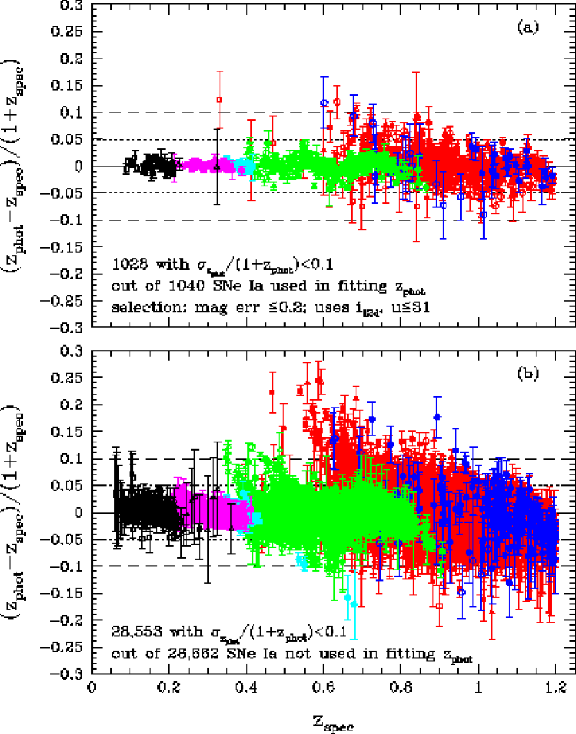
Figure 1: The performance of the analytic photo-z estimator applied to simulated SNe from the LSST, as indicated by $(z_{\rm phot}-z_{\rm spec})/(1+z_{\rm spec})$ versus $z_{\rm spec}$, with cut $\sigma_{z_{\rm phot}}/(1+z_{\rm phot})<0.1$ for cleaner presentation (the numbers of outliers are given in Table 1).. Different colors indicate SNe with different photometric passbands, as described in Table 1. For SNe represented by the same color, different point types represent subdivisions based on brightness to improve precision.

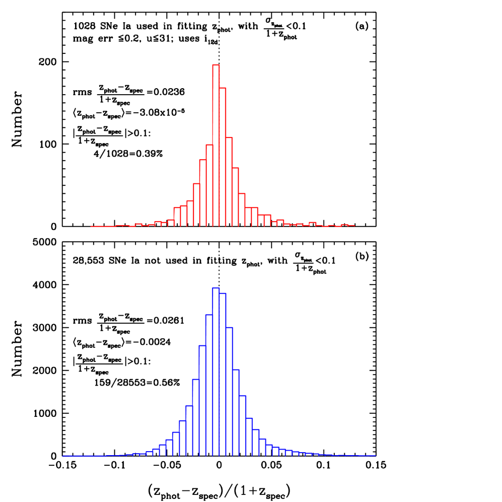
Figure 2: The distribution of $(z_{\rm phot}-z_{\rm spec})/(1+z_{\rm spec})$ from Fig.1.

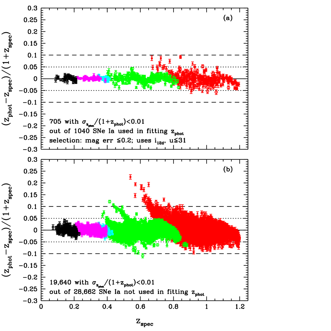
Figure 3: The same as Fig.1, but with cut $\sigma_{z_{\rm phot}}/(1+z_{\rm phot})<0.01$ for improved accuracy, precision, and outlier reduction.

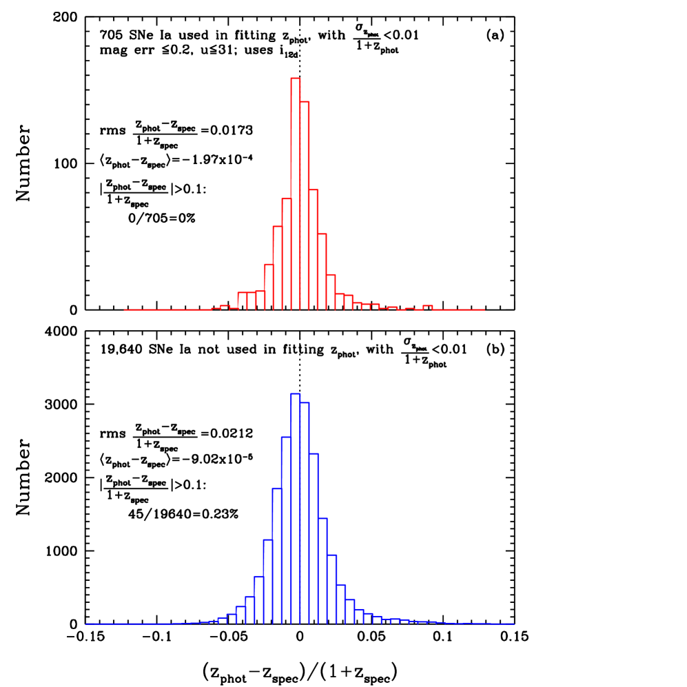
Figure 4: The distribution of $(z_{\rm phot}-z_{\rm spec})/(1+z_{\rm spec})$ from Fig.3.

Table 2 shows that we can arrive at photo-z’s with higher accuracy, precision, and purity by using the estimated errors on $z_{\rm phot}$ to exclude SNe with large $\sigma_{z_{\rm phot}}/(1+z_{\rm phot})$. If we exclude SNe with $\sigma_{z_{\rm phot}}/(1+z_{\rm phot})\geq 0.01$, we arrive at a precision of $\sigma(z_{\rm phot}-z_{\rm spec})/(1+z_{\rm spec})=0.02$, a bias in $z_{\rm phot}$ (the mean of $z_{\rm phot}-z_{\rm spec}$) of $-9\times 10^{-5}$, and an outlier fraction (with $\left|(z_{\rm phot}-z_{\rm spec})/(1+z_{\rm spec})\right|>0.1$) of 0.23 percent (see Fig.3). Note that for the threshold of $\sigma_{z_{\rm phot}}/(1+z_{\rm phot})<0.01$, there are no outliers in the training set. We can require that there are no outliers in the training set in order to arrive at this threshold for $\sigma_{z_{\rm phot}}/(1+z_{\rm phot})$.

4.2 Photo-z’s using SN Ia colors only

As we discussed in Sec.2.3, having an alternative photometric redshift estimator that uses SN Ia colors only is helps increase the robustness of cosmological constraints obtained using photometric SNe Ia. Table 1 tabulates the resultant precision and accuracy of our photo-z estimator using SN Ia colors only, for each color group. The colors only results are tabulated immediately below the results for colors plus $i$ band peak flux (see the previous subsection), and indicated by “Y” under the column for “colors only”. Using SN colors only leads to slightly worse precision, but similar accuracy for the resultant photo-z’s.

Fig.5 and Fig.7 are results corresponding to Fig.1 and Fig.3, but for $z_{phot}$ obtained using Eq.(7), which uses SN Ia colors only. Using the SN Ia colors only, we obtain a set of photo-z’s with similar quality to using SN Ia color and $i$ band peak flux by requiring that $\sigma_{z_{\rm phot}}/(1+z_{\rm phot})<0.007$; this leads to a set of photo-z’s with 2 percent accuracy, a bias in $z_{\rm phot}$ of $5.9\times 10^{-4}$, and an outlier fraction of 0.32%. The threshold level of $\sigma_{z_{\rm phot}}/(1+z_{\rm phot})<0.007$ is set naturally by requiring that there are no outliers in the training set. There are 58 outliers (with $\left|(z_{\rm phot}-z_{\rm spec})/(1+z_{\rm spec})\right|>0.1$) in the second panel from the top in Fig.7 (the majority are from the rizY color groups G11 through G15 — similar to Fig.3), representing 0.32% of all 18,370 SNe Ia from the test sample that passed this cut. We do not expect such a small fraction of outliers to have noticeable impact on the cosmological fit; we will investigate this in future work.

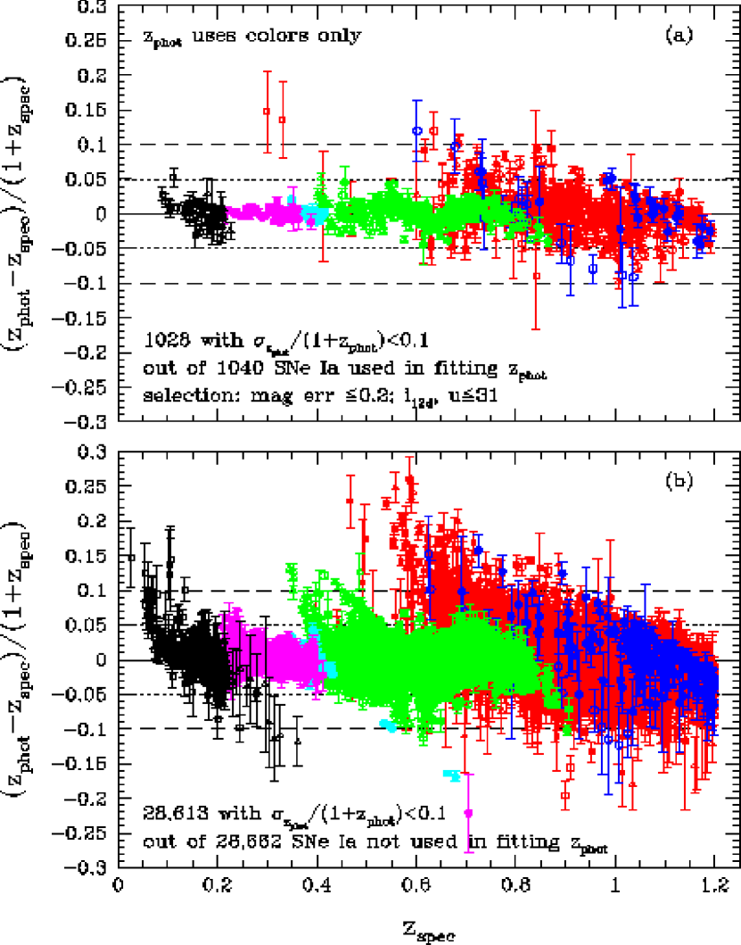
Figure 5: The same as Fig.1, but for $z_{\rm phot}$ obtained using SN Ia colors only.

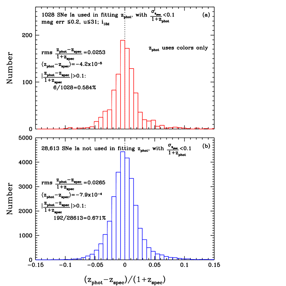
Figure 6: The distribution of $(z_{\rm phot}-z_{\rm spec})/(1+z_{\rm spec})$ from Fig.5.

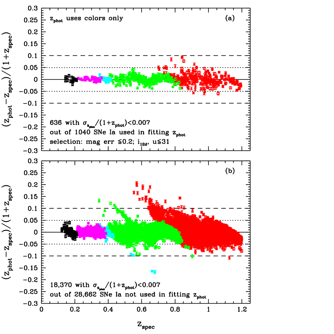
Figure 7: The same as Fig.5, but with cut $\sigma_{z_{\rm phot}}/(1+z_{\rm phot})<0.007$ for improved accuracy, precision, and outlier reduction.

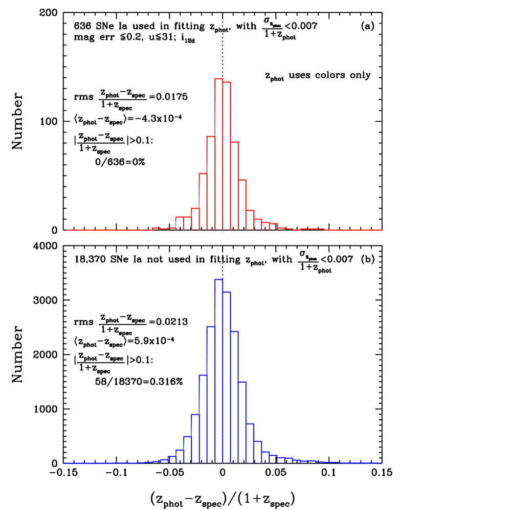
Figure 8: The distribution of $(z_{\rm phot}-z_{\rm spec})/(1+z_{\rm spec})$ from Fig.7.

5 Summary and Discussion

We have shown that a simple analytic photo-z estimator for SNe Ia can be built for the LSST, given suitably chosen training sets of SNe Ia with spectroscopic redshifts that are representative of the general properties of SNe Ia from the LSST. While our method is based on that proposed by Wang (2007), and advanced by Wang, Narayan, & Wood-Vasey (2007), it represents a significant improvement over previous work (which require the use of both colors and $i$ magnitudes of SNe Ia) in enabling the use of SN Ia colors only. This eliminates the possible complications that can arise from using SN Ia brightness in estimating photo-z’s, since the peak brightness of a SN Ia is closely correlated with its distance from us.

Our sample of simulated LSST SNe Ia is representative of data expected from the LSST, based on our current knowledge of SNe Ia. The multiple-band photometry from the LSST enables us to divide the SNe Ia into different sets (see Sec.2.2 and Table 1). For each set, a photo-z estimator is constructed using only quadratic functions of colors (see Eq.[7]), with the constant coefficients given by fitting to a training set that contains a maximum of 100 SNe Ia with spectroscopic redshifts (see Table 1). Note that the division of SNe Ia into color groups is empirical, dependent on the properties of the training set, assumed to be representative of the overall sample.

In addition to how the photometric SNe Ia should be grouped, and the performance of our photo-z estimator for each color group, Table 1 contains other helpful information as well. As expected, the performance of the photo-z estimator improves with the increasing number of filters in which photometric data are available; note that knowing the filters in which the SNe Ia are visible provides a crude estimate of the redshift range of the SNe Ia. Not surprisingly, the performance of the photo-z estimator generally degrades with the increasing redshift of the SNe Ia.

While Table 1 lists all the SNe Ia that passed our data quality cut (see Sec.3), Table 2 shows us how to derive a high purity sample of photo-z’s by making cuts on the SNe Ia based on the estimated errors of the photo-z’s. This is very useful since we are systematics limited, rather than statistics limited, in using photometric SNe Ia for cosmology.

The performance of our simple analytic SN Ia photo-z estimator is quite impressive when applied to simulated LSST SN Ia photometric data (see Table 2). We find that the estimated errors on the photo-z’s, $\sigma_{z_{\rm phot}}/(1+z_{\rm phot})$, can be used as filters to produce a set of photo-z’s that have high precision, accuracy, and purity. Using SN Ia colors as well as SN Ia peak magnitude in the $i$ band, we obtain a set of photo-z’s with 2 percent accuracy (with $\sigma(z_{\rm phot}-z_{\rm spec})/(1+z_{\rm spec})=0.02$), a bias in $z_{\rm phot}$ (the mean of $z_{\rm phot}-z_{\rm spec}$) of $-9\times 10^{-5}$, and an outlier fraction (with $\left|(z_{\rm phot}-z_{\rm spec})/(1+z_{\rm spec})\right|>0.1$) of 0.23 percent, with the requirement that $\sigma_{z_{\rm phot}}/(1+z_{\rm phot})<0.01$. Using the SN Ia colors only, we obtain a set of photo-z’s with similar quality by requiring that $\sigma_{z_{\rm phot}}/(1+z_{\rm phot})<0.007$; this leads to a set of photo-z’s with 2 percent accuracy, a bias in $z_{\rm phot}$ of $5.9\times 10^{-4}$, and an outlier fraction of 0.32 percent.

In future work, we will investigate whether the precision and accuracy achieved by our photo-z estimator is adequate for cosmology, We will first need to simulatte more realistic samples of LSST SNe, which include non-Ia’s. We will need to expand and advance our photo-z estimator for weeding out non-Ia SNe. There is much work to do before our photo-z estimator can be applied to the real LSST data.

In principle, our method for estimating photo-z’s should be applicable to other surveys, but its performance depends on the precision of the photometry of the surveys. However, it can still be used as a quick way of estimating photo-z’s that is model-independent, and complementary to the template-based methods. The application of our method to non-Ia SNe and galaxies can also be explored. This method for estimating photo-z’s for SNe Ia was initially inspired by a similar method for estimating galaxy redshifts presented by Wang, Bahcall, & Turner (1998). It would be interesting to develop a simple photo-z estimator for LSST galaxies based on this method.

We expect that our SN photo-z estimator for the LSST will be useful in probing dark energy using LSST SNe Ia with photometry only. It will also provide an independent cross-check for SN photo-z’s derived from other, template-based photo-z estimators (see, e.g., Kim & Miquel (2007); Kessler et al. (2010a); Palanque-Delabrouille (2010)). Our linear photo-z model is very convenient for propagating photometric uncertainties, especially compared to more “black-box” type machine learning algorithms. In future work, we will examine the cosmological constraints that can be obtained using LSST SNe Ia with photometry only, with photo-z’s estimated using the method presented in this paper.

set	bands	subdivision	symbol in Fig.1	$N_{s}$	$N_{test}$	colors	$\sigma\left[\frac{\Delta z}{1+z}\right]$	$\langle z_{\rm phot}-z\rangle$	outliers	flagged
			& Fig.5			only	training, test	training, test	training, test	in test
G11	$rizY$	$i\geq 24.8$	red filled circles	100	2904	N	.0255,   .0299	$-$2.6E-7, $\,-$.0074	0, 22	15
						Y	.0264,  .0261	$-$1.6E-7, $\,-$.0032	0, 8	0
G12	$rizY$	$i=[24.5,24.8)$	red empty circles	100	3060	N	.0308,  .0280	$-$8.1E-8, $\,-$.0039	1, 11	0
						Y	.0313,   .0280	$-$6.0E-7, $\,-$.0051	1, 14	0
G13	$rizY$	$i=[24,24.5)$, $r\geq 25.2$	red filled triangles	100	4184	N	.0274,  .0290	2.5E-7, $\,-$.0017	0, 25	0
						Y	.0280,  .0289	$-$1.0E-7, $\,-$8.7E-4	1, 26	0
G14	$rizY$	$i=[24,24.5)$, $r<25.2$	red empty triangles	100	1505	N	.0301,   .0369	1.1E-7,   3.5E-5	1, 23	4
						Y	.0306,   .0362	$-$6.5E-8,   6.1E-4	1, 22	2
G15	$rizY$	$i=[23,24)$	red filled squares	100	4900	N	.0279,   .0346	1.1E-7, $\,-$8.5E-4	0, 75	0
						Y	.0292,   .0352	$-$3.2E-7,   .0021	0, 92	0
G16	$rizY$	$i<23$	red empty squares	40	53	N	.0408,   .0526	$-$7.1E-8, $\,-$.033	1, 4	2
						Y	.0494,   .0612	$-$2.6E-8, $\,-$.039	2, 5	3
G21	$izY$	$i\geq 24.5$	blue filled circles	20	174	N	.0202,   .0472	$-$1.0E-7, $\,-$.0097	0, 6	0
						Y	.0251,   .0393	1.4E-8,   .0032	0, 3	0
G22	$izY$	$i<24.5$	blue empty circles	20	18	N	.055,   .108	$-$1.3E-8, $\,-$.068	1, 7	2
						Y	.0627,   .0798	4.3E-8, $\,-$.0508	2, 5	0
G31	$grizY$	$i\geq 23.5$	green filled circles	100	2508	N	.0163,   .0196	$-$1.5E-7,   .0023	0, 3	2
						Y	.0165,   .0192	$-$3.0E-8,   .0035	0, 1	0
G32	$grizY$	$i=[23.1,23.5)$	green empty circles	100	3242	N	.0122,   .0155	2.1E-7, $\,-$.0027	0, 2	0
						Y	.0125,   .0157	1.6E-7, $\,-$.0016	0, 3	0
G33	$grizY$	$i<23.1$	green empty triangles	100	3888	N	.0137,   .0179	2.0E-7, $\,-$.0069	0, 4	0
						Y	.0151,   .0183	$-$3.8E-8, $\,-$.0025	0, 6	0
G4	$griz$		cyan filled circles	50	480	N	.0055,   .0229	2.7E-8,   .0018	0, 8	6
						Y	.0059,   .0421	$-$5.7E-8,   .0088	0, 11	9
G5	$ugriz$		magenta filled circles	50	1361	N	.0048,   .0094	$-$1.9E-8, $\,-$5.2E-4	0, 1	1
						Y	.0063,   .0123	7.2E-8,   9.6E-4	0, 1	0
G61	$ugri$	$r\geq 21$	black empty triangles	20	75	N	.0049,   .048	$-$1.1E-7,   .0091	0, 4	4
						Y	.0097,   .0507	$-$2.1E-8, $\,-$.010	0, 4	1
G62	$ugri$	$r<21$	black empty squares	40	310	N	.0082,   .026	$-$2.1E-7,   .0019	0, 1	1
						Y	.0168,   .0319	8.5E-9,   .0039	0, 6	1

Table 1: Division of SNe into sets according to available photometric passbands, and into subsets in each set for improved precision. The “outliers” column indicates the number of SNe in the training set and test set that have $\left|(z_{\rm phot}-z_{\rm spec})/(1+z_{\rm spec})\right|>0.1$. The “flagged in test” column indicates the number of outliers in the test set that have $\sigma_{z_{\rm phot}}/(1+z_{\rm phot})\geq 0.1$.

set	$\frac{\sigma_{z_{mphot}}}{1+z_{mphot}}<$	colors only	$N_{tot}$	$N_{cut}$	$\sigma\left[\frac{\Delta z}{1+z}\right]$	$\langle z_{\rm phot}-z\rangle$	flagged outlier	outliers
training	100	N	1040	0	.0241	$-$9.6E-8	0	4
		Y	1040	0	.0259	$-$1.8E-6	0	7
test	100	N	28662	0	.0270	$-$.0027	0	196 (0.68%)
		Y	28662	0	.0271	$-6.9\times 10^{-4}$	0	207 (0.72%)
training	0.1	N	1028	12	.0236	$-$3.1E-5	0	4
		Y	1028	12	.0253	$-$4.2E-5	1	6
test	0.1	N	28553	109	.0261	$-$.0024	37	159 (0.56%)
		Y	28613	49	.0265	$-7.9\times 10^{-4}$	15	192 (0.67%)
training	0.05	N	1011	29	.0229	$-$.00022	1	3
		Y	1017	23	.0242	$-$5.1E-4	3	4
test	0.05	N	28327	335	.0257	$-$.0021	53	143 (0.50%)
		Y	28499	163	.0262	$-6.8\times 10^{-4}$	31	176 (0.62%)
training	0.02	N	918	122	.0204	$-$.00073	3	1
		Y	949	91	.0221	$-$3.0E-4	5	2
test	0.02	N	26606	2056	.0242	$-$.0010	95	101 (0.38%)
		Y	27480	1182	.0250	$-3.0\times 10^{-4}$	74	133 (0.48%)
training	0.01	N	705	335	.0173	$-$.00020	4	0
	0.007	Y	636	404	.0175	$-$4.3E-4	7	0
test	0.01	N	19640	9022	.0212	$-$9.0E-5	151	45 (0.23%)
	0.007	Y	18370	10292	.0213	$5.9\times 10^{-4}$	149	58 (0.32%)

Table 2: Obtaining sets of photo-z’s with higher accuracy, precision, and purity by using the estimated errors on $z_{\rm phot}$ to exclude SNe with large $\sigma_{z_{\rm phot}}/(1+z_{\rm phot})$.

References

- (1)
- Abell et al. (2009) Abell, P. A. et al. 2009, e-prints arXiv:0912.0201
- Albrecht et al. (2006) Albrecht, A., et al., Report of the Dark Energy Task Force; available online at arXiv:astro-ph/0609591v1
- Astier et al. (2006) Astier, P., et al. 2006, A & A 447, 31-48 (2006)
- Bernstein et al. (2012) Bernstein, J.P. et al., Astrophysical Journal 753 (2012) 152
- Caldwell & Kamionkowski (2009) Caldwell, R. R., & Kamionkowski, M., 2009, Ann.Rev.Nucl.Part.Sci., 59, 397
- Campbell et al. (2013) Campbell, H., et al., 2013, ApJ, 763, 88
- Dilday et al. (2008) Dilday, B., et al., 2008, ApJ, 682, 262
- Frieman, Turner, & Huterer (2008) Frieman, J., Turner, M., Huterer, D., ARAA, 46, 385 (2008)
- Guzzo et al. (2008) Guzzo, L., et al., 2008, Nature, 451, 541
- Guy et al. (2007) Guy, J. et al. 2007, Astronomy & Astrophysics, 466, 11
- Guy et al. (2010) Guy, J. et al. 2010, Astronomy & Astrophysics, 523, A7
- Hlozek et al. (2012) Hlozek, R., et al., 2012, ApJ, 752, 79
- Kessler et al. (2009a) Kessler, R. et al. 2009a, ApJS, 185, 32
- Kessler et al. (2009b) Kessler, R. et al. 2009b, PASP, 121, 1028
- Kessler et al. (2010a) Kessler, R. et al., 2010, ApJ, 717, 40
- Kessler et al. (2010b) Kessler, R.; Conley, A.; Jha, S.; Kuhlmann, S., arXiv:1001.5210 [astro-ph.IM]
- Kim & Miquel (2007) Kim, A. G.; Miquel, R., 2007, Astroparticle Physics, 28, 448
- Knox, Song, & Tyson (2006) Knox, L.; Song, Y.-S.; Tyson, J. A., 2006, PRD, 74, 023512
- Li et al. (2011) Li, M.; Li, X.-D.; Wang, S.; Wang, Y., 2011, Commun.Theor.Phys., 56, 525
- Lupton (1993) Lupton, R., 1993, “Statistics in Theory and Practice”, Princeton University Press
- Palanque-Delabrouille (2010) Palanque-Delabrouille, N., et al., 2010, A & A, 514, A63
- Perlmutter et al. (1999) Perlmutter, S., et al., Astrophysical Journal 517 (1999) 565
- Ratra & Vogeley (2008) Ratra, B., Vogeley, M. S., 2008, Publ.Astron.Soc.Pac., 120, 235
- Riess et al. (1998) Riess, A., et al., Astron.J. 116 (1998) 109
- Sako et al. (2011) Sako, M., Bassett, B., Connolly, B., et al. 2011, ApJ, 738, 162
- Uzan (2010) Uzan, J.-P. 2010, General Relativity and Gravitation, 42, 2219
- Wang, Bahcall, & Turner (1998) Wang, Y.; Bahcall, N.; Turner, E. L., 1998, AJ, 116, 2081
- Wang (2007) Wang, Y., 2007, ApJ Lett., 654, 123
- Wang (2008) Wang, Y. , 2008, JCAP, 05, 021
- Wang (2010) Wang, Y., Dark Energy, Wiley-VCH (2010)
- Wang, Narayan, & Wood-Vasey (2007) Wang, Y.; Narayan, G.; Wood-Vasey, M., 2007, MNRAS, 382, 377 (2007)
- Weinberg et al. (2013) Weinberg, D. H.; Mortonson, M. J.; Eisenstein, D.J.; Hirata, C.; Riess, A. G.; Rozo, E 2013, Physics Reports, 530, 87