Why do mixed quantum-classical methods describe short-time dynamics through conical intersections so well? Analysis of geometric phase effects

Abstract

Adequate simulation of non-adiabatic dynamics through conical intersection requires account for a non-trivial geometric phase (GP) emerging in electronic and nuclear wave-functions in the adiabatic representation. Popular mixed quantum-classical (MQC) methods, surface hopping and Ehrenfest, do not carry a nuclear wave-function to be able to incorporate the GP into nuclear dynamics. Surprisingly, the MQC methods reproduce ultra-fast interstate crossing dynamics generated with the exact quantum propagation so well as if they contained information about the GP. Using two-dimensional linear vibronic coupling models we unravel how the MQC methods can effectively mimic the most significant dynamical GP effects: 1) compensation for repulsive diagonal second order non-adiabatic couplings and 2) transfer enhancement for a fully cylindrically symmetric component of a nuclear distribution.

I Introduction

The Born-Oppenheimer representation of the electron-nuclear wave-function introduces natural separation between time/energy scales of electrons and nuclei in molecular systems. This separation allows one to consider nuclear dynamics independently from that of the electronic subsystem reducing the number of involved degrees of freedom (DOF). This representation is uniquely defined through the electronic eigenvalue problem with fixed nuclei and is conveniently available in numerous electronic structure packages. However, there are also a few complications associated with the inherent non-separability of dynamics in a general interacting many-body system. For example in many photochemical processes nuclear molecular dynamics cannot be adequately modelled on a single potential energy surface (PES) because for some nuclear configurations the separation between electronic PESs becomes comparable to the nuclear energy scale or even vanishes. The latter case often presents itself in the form of conical intersections (CIs).Truhlar and Mead (2003); Migani and Olivucci (2004) Non-adiabatic dynamics associated with such crossings not only results in transferring system population between electronic states but also in geometric phase (GP) effects.Schön and Köppel (1995); Ryabinkin and Izmaylov (2013); Baer et al. (1996); Ryabinkin, Joubert-Doriol, and Izmaylov (2014); Althorpe, Stecher, and Bouakline (2008); Bouakline (2014) The latter is caused by a nontrivial nuclear dependent geometric or Berry phase appearing in both nuclear $\chi_{j}(\mathbf{R},t)$ and electronic $\Phi_{j}(\mathbf{r};\mathbf{R})$ wave-functions within the adiabatic representation of the total electron-nuclear wave-functionCederbaum (2004)

$$\Psi(\mathbf{r},\mathbf{R},t) = \sum_{j}\Phi_{j}(\mathbf{r};\mathbf{R})\chi_{j}(\mathbf{R},t).$$ (1)

BerryBerry (1984) and Longuet-HigginsLonguet-Higgins et al. (1958) have shown that parametric evolution of the electronic parts $\Phi_{j}(\mathbf{r};\mathbf{R})$ around the point of eigenvalue degeneracies (the CI seam) must change their signs, which makes $\Phi_{j}(\mathbf{r};\mathbf{R})$ double-valued functions of nuclear DOF $\mathbf{R}$. To preserve the single-valued character of the total wave-function, $\Psi(\mathbf{r},\mathbf{R},t)$, the nuclear part, $\chi_{j}(\mathbf{R},t)$, must also have a double-valued character compensating that in the electronic components. GPs in electronic wave-functions $\Phi_{j}(\mathbf{r};\mathbf{R})$ are needed to obtain non-adiabatic couplings (NACs)$\bra{\Phi_{i}(\mathbf{R})}\nabla_{\mathbf{R}}\Phi_{j}(\mathbf{R})\rangle_{\mathbf{r}}$ and $\bra{\Phi_{i}(\mathbf{R})}\nabla_{\mathbf{R}}^{2}\Phi_{j}(\mathbf{R})\rangle_{\mathbf{r}}$ correctly,Ben-Nun and Martinez (2002) but NACs alone are not sufficient for simulating nuclear dynamics properly. For the correct dynamics near CIs, the nuclear part must also have the GP resulting in double-valued nuclear wave-functions $\chi_{j}(\mathbf{R})$. Ignoring the GP of nuclear wave-functions can lead to qualitative distortion of non-adiabatic dynamics even in the the absence of a significant population transfer between crossing electronic states.Schön and Köppel (1995); Baer et al. (1996); Ryabinkin and Izmaylov (2013); Joubert-Doriol, Ryabinkin, and Izmaylov (2013) Interestingly, dynamical features associated with the GP are very different for low energy dynamics (Fig. 1a) and excited state dynamics (Fig. 1b). The main manifestation of GP effects in low energy nuclear dynamics is destructive interference between two paths around the CI seam (Fig. 1a),Schön and Köppel (1995); Ryabinkin and Izmaylov (2013); Joubert-Doriol, Ryabinkin, and Izmaylov (2013) while in the excited state dynamics (Fig. 1b), it is enhancement of population transfer for a fully cylindrical component of a nuclear wave-packet and compensation of a repulsive diagonal Born-Oppenheimer correction (DBOC), $\bra{\Phi_{i}(\mathbf{R})}\nabla_{\mathbf{R}}^{2}\Phi_{i}(\mathbf{R})\rangle_{\mathbf{r}}$.Ryabinkin, Joubert-Doriol, and Izmaylov (2014)

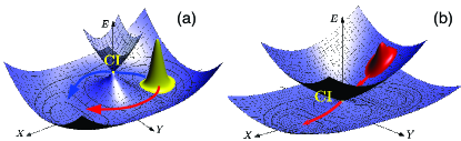
Figure 1: Low energy (a) and excited state (b) nuclear dynamics near CI.

The DBOC is usually neglected in non-adiabatic simulations for molecular systems based on its small value near the minimum of the ground state. However, at the intersecting manifold this term diverges to infinity (see Fig. 2), and its a priori neglect is not justified.

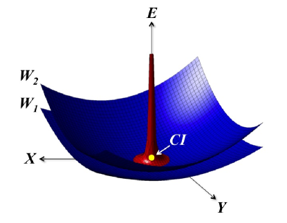
Figure 2: Near CIs, the DBOC becomes very large and alters electronic PESs. In the absence of the GP, the DBOC can inhibit the access of a nuclear-wave packet to the CI.

One of the most popular ways to simulate non-adiabatic dynamics near CIs in large systems is using mixed quantum-classical (MQC) approaches: surface hopping (SH) and Ehrenfest (EF) methods.Tully (1990, 1998) Unlike full quantum approaches, MQC methods propagate nuclear DOF classically. As a result, they exhibit some well-known limitations of classical mechanics such as inability to model nuclear tunnelling and quantum interference effects. The GP induced destructive interference in low energy dynamics (Fig. 1a) is a typical example of the latter effect. MQC methods have only the electronic part of the wave-function and thus cannot fully account for the GP, because even though the electronic function acquires the GP through parametric dependence on nuclear evolution, nuclei evolve according to classical Newton equations that do not have any GP contributions. In this context, it is quite surprising that short-time excited state deactivation dynamics (Fig. 1b) of MQC methods agrees extremely well with that of the exact quantum propagationMüller and Stock (1997); Worth, Hunt, and Robb (2003); Barbatti et al. (2007) for systems where GP effects were proven to be very influential.Ryabinkin, Joubert-Doriol, and Izmaylov (2014)

In this work we will explain how MQC methods emulate GP effects in CI problems. We will restrict our attention to GP effects in excited state deactivation process (Fig. 1b). As for low energy dynamics (Fig. 1a), SH and EF methods are not much better than a simple classical dynamics because non-adiabatic transitions are well suppressed by the energy difference in areas accessible for classical trajectories. Currently, only the quantum-classical Liouville formalism has proven to be capable to capture GP effects in low energy dynamics.Ryabinkin et al. (2014)

The rest of the paper is organized as follows. First, we introduce a diabatic two-dimensional linear vibronic coupling (LVC) model, although very simple representation of the CI topology, this model has all quantities involved in quantum and MQC simulations in the analytical form. Thus, it allows us to compare various quantum and MQC methods on the same footing and to reveal the key components of the MQC schemes that are responsible for mimicking quantum GP effects. Second, to confirm our analysis we simulate non-adiabatic dynamics for a few molecular systems that provide a variety of dynamical regimes. Finally, we conclude the paper with a summary and further ramifications of our work.

II Theory

II.1 2D LVC model

The GP appears only in the adiabatic representation, however, it is more convenient to start with a model in the diabatic representation because a diabatic model will allow us to obtain the GP explicitly.Mead and Truhlar (1979) Moreover, the diabatic representation can be exactly transformed to the adiabatic representation while the exact reverse transformation does not exist in general.Mead and Truhlar (1982) Note that although diabatic wave-functions do not have GPs, simulations in the diabatic representation incorporate all GP effects implicitly and are considered to be exact. Thus, we start with introducing a diabatic model Hamiltonian

$$H_{\rm 2D}=T_{\rm 2D}{\mathbf{1}}_{2}+\begin{pmatrix}V_{11}&V_{12}\\ V_{12}&V_{22}\end{pmatrix},$$ (2)

where $T_{\rm 2D}=-\hbar^{2}2^{-1}(\partial^{2}/\partial x^{2}+\partial^{2}/\partial y^{2})$ is the nuclear kinetic energy operator, $x$ and $y$ are mass-weighted nuclear coordinates, $V_{11}$ and $V_{22}$ are the diabatic potentials represented by identical two-dimensional parabolas shifted in space and coupled by the $V_{12}$ potential

$$V_{11}={} \dfrac{1}{2}\left[\omega_{1}^{2}(x+x_{0})^{2}+\omega_{2}^{2}y^{2}\right],\quad V_{12}=cy,$$ (3)

$$V_{22}={} \dfrac{1}{2}\left[\omega_{1}^{2}(x-x_{0})^{2}+\omega_{2}^{2}y^{2}\right].$$ (4)

Here, $\omega_{i}$’s are harmonic frequencies for nuclear coordinates $x$ and $y$, $\pm x_{0}$ are the minima of $V_{11}$ and $V_{22}$ potentials, and $c$ is a coupling constant. Electronic DOF in $H_{\rm 2D}$ are vectors $|{}\phi_{1}^{\rm dia}\rangle$ and $|{}\phi_{2}^{\rm dia}\rangle$ in a two-dimensional linear space. To obtain the corresponding adiabatic representation for the Hamiltonian $H_{\rm 2D}$ one needs to diagonalize the two-state potential matrix in Eq. (2) by a unitary transformation that defines the adiabatic electronic states as

$$|{}\phi_{1}^{\text{adi}}\rangle = \phantom{-}\cos\frac{\theta}{2}\,|{}\phi_{1}^{\rm dia}\rangle+\sin\frac{\theta}{2}\,|{}\phi_{2}^{\rm dia}\rangle,$$ (5)

$$|{}\phi_{2}^{\text{adi}}\rangle = -\sin\frac{\theta}{2}\,|{}\phi_{1}^{\rm dia}\rangle+\cos\frac{\theta}{2}\,|{}\phi_{2}^{\rm dia}\rangle,$$ (6)

where

$$\theta=\arctan\dfrac{2\,V_{12}}{V_{11}-V_{22}}$$ (7)

is a mixing angle between the diabatic states $|{}\phi_{i}^{\rm dia}\rangle$. The adiabatic functions $|{}\phi_{i}^{\text{adi}}\rangle$ are double-valued functions of the nuclear parameters $(x,y)$ because encircling the CI point corresponds to change in $\theta(x,y)$ from 0 to 2$\pi$ which leads to a sign change in $|{}\phi_{i}^{\text{adi}}\rangle$. The unitary transformation to the adiabatic representation brings $H_{\rm 2D}$ to a form

$${H}_{\rm 2D}^{\text{adi}}=\begin{pmatrix}T_{\rm 2D}+\tau_{11}&\tau_{12}\\ \tau_{21}&T_{\rm 2D}+\tau_{22}\end{pmatrix}+\begin{pmatrix}W_{1}&0\\ 0&W_{2}\end{pmatrix},$$ (8)

where

$$W_{1,2}= {}\dfrac{1}{2}\left(V_{11}+V_{22}\right)\mp\dfrac{1}{2}\sqrt{\left(V_{11}-V_{22}\right)^{2}+4V_{12}^{2}},$$ (9)

are the adiabatic potentials with the minus (plus) sign for $W_{1}$ ($W_{2}$), and

$$\tau_{ij} = -\hbar^{2}\mathbf{d}_{ij}\cdot\nabla-\frac{\hbar^{2}}{2}D_{ij},$$ (10)

are kinetic energy terms containing NACs

$$\mathbf{d}_{ij} = \bra{\phi_{i}^{\text{adi}}}\nabla\phi_{j}^{\text{adi}}\rangle,\quad D_{ij}=\bra{\phi_{i}^{\text{adi}}}\nabla^{2}\phi_{j}^{\text{adi}}\rangle$$ (11)

with $\nabla=(\partial/\partial x,\partial/\partial y)$. Substituting definitions of the adiabatic states into Eq. (10), $\hat{\tau}_{ij}$ can be express as

$$\hat{\tau}_{ii} = -\frac{\hbar^{2}D_{ii}}{2}=\frac{\hbar^{2}(x^{2}+y^{2})}{8(\gamma^{-1}x^{2}+\gamma y^{2})^{2}},\quad\gamma=\frac{c}{x_{0}\omega_{1}^{2}}$$ (12)

$$\hat{\tau}_{ij} = \frac{\hbar(\overrightarrow{\hat{L}}_{z}-\overleftarrow{\hat{L}}_{z})}{4(\gamma^{-1}x^{2}+\gamma y^{2})},\quad i\neq j$$ (13)

where $\hat{L}_{z}=-i\hbar(x\partial/\partial y-y\partial/\partial x)$ is the angular momentum operator, and the overhead arrows indicate operator’s directionality.

In quantum dynamics within the adiabatic representation, the GP can be introduced as a position-dependent phase factor $e^{i\theta(x,y)/2}$ for single-valued nuclear basis functions, where $\theta(x,y)$ is provided by Eq. (7).Mead and Truhlar (1979) This phase factor would change signs of nuclear wave-functions on encircling the CI. However, it is more convenient to use this factor as a unitary transformation of the adiabatic Hamiltonian: $\hat{H}^{\text{GP}}_{2D}=e^{-i\theta/2}\hat{H}^{\text{adi}}_{2D}e^{i\theta/2}$, then for simulating GP effects we can use a normal single-valued nuclear basis with the $\hat{H}^{\text{GP}}_{2D}$ Hamiltonian. Also this approach allows one to compare $\hat{H}^{\text{adi}}_{2D}$ and $\hat{H}^{\text{GP}}_{2D}$ to see what operator terms are responsible for introducing GP effects. The comparison reveals that the phase factor alters kinetic energy terms

$$\hat{\tau}^{\text{GP}}_{ii} = \frac{\hbar(\overrightarrow{\hat{L}}_{z}-\overleftarrow{\hat{L}}_{z})}{4(\gamma^{-1}x^{2}+\gamma y^{2})}+\frac{\hbar^{2}(x^{2}+y^{2})}{4(\gamma^{-1}x^{2}+\gamma y^{2})^{2}},$$ (14)

$$\hat{\tau}^{\text{GP}}_{ij} = \frac{\hbar(\overrightarrow{\hat{L}}_{z}-\overleftarrow{\hat{L}}_{z})}{4(\gamma^{-1}x^{2}+\gamma y^{2})}-\frac{\hbar^{2}(x^{2}+y^{2})}{4(\gamma^{-1}x^{2}+\gamma y^{2})^{2}},~{}i\neq j$$ (15)

and thus changes probabilities of electronic transitions.

II.2 Mixed quantum-classical methods

One of the most straightforward routes to the MQC methods is to take the classical limit for nuclear DOF in the system wave-function, then for a two-state problem within the adiabatic representation an electronic wave-function is given

$$\psi_{e}(\mathbf{r};\mathbf{R},t)=\sum_{j=1}^{2}c_{j}(t)\phi_{j}^{\rm adi}(\mathbf{r};\mathbf{R}(t)).$$ (16)

The time-dependent coefficients are obtained from projection of the electronic time-dependent Schrödingier equation (TDSE)

$$i\hbar\sum_{j=1}^{2}[\dot{c}_{j}\phi_{j}^{\rm adi}+c_{j}\dot{\phi}_{j}^{\rm adi}]=\sum_{k=1}^{2}c_{k}W_{k}(\mathbf{R})\phi_{k}^{\rm adi}$$ (17)

onto the electronic adiabatic basis $\phi_{j}^{\rm adi}(\mathbf{r};\mathbf{R}(t))$

$$i\hbar\begin{pmatrix}{\dot{c}_{1}}\\ {\dot{c}_{2}}\end{pmatrix}=\begin{pmatrix}W_{1}(\mathbf{R})&-i\hbar\mathbf{d}_{12}\cdot\dot{\mathbf{R}}\\ -i\hbar\mathbf{d}_{21}\cdot\dot{\mathbf{R}}&W_{2}(\mathbf{R})\end{pmatrix}\begin{pmatrix}{{c}_{1}}\\ {{c}_{2}}\end{pmatrix}.$$ (18)

Here, the chain rule for NACs is used

$$\bra{\phi_{j}^{\rm adi}(\mathbf{R}(t))}\dot{\phi}_{i}^{\rm adi}(\mathbf{R}(t))\rangle=\dot{\mathbf{R}}\cdot\mathbf{d}_{ji}.$$ (19)

Thus, due to orthogonality of the adiabatic states the system population of each electronic state is given by $|c_{i}(t)|^{2}$ and the population transfer is regulated by the off-diagonal elements $-i\hbar\mathbf{d}_{12}\cdot\dot{\mathbf{R}}$ in Eq. (18).

The nuclear equations of motion (EOM) for the EF method are derived from the total energy conservation condition

$$\frac{dE}{dt}=\frac{d}{dt}\left(\frac{\mathbf{P}^{2}}{2}+\mathbf{c}^{\dagger}\mathbf{H}_{\rm adi}^{(e)}\mathbf{c}\right)=0,$$ (20)

with $[\mathbf{H}_{\rm adi}^{(e)}]_{ij}=\delta_{ij}W_{i}(\mathbf{R})$, which leads to Newton’s EOM for nuclei

$$\ddot{R}_{\alpha}=-\mathbf{c}^{\dagger}\frac{\partial{\mathbf{H}_{\rm adi}^{(e)}}}{\partial{R_{\alpha}}}\mathbf{c}+\mathbf{c}^{\dagger}[\mathbf{H}_{\rm adi}^{(e)},\mathbf{d}_{\alpha}]\mathbf{c},$$ (21)

where

$$\mathbf{d}_{\alpha} = \begin{pmatrix}0&\braket{\phi_{1}^{\rm adi}}{\frac{\partial\phi_{2}^{\rm adi}}{\partial{R_{\alpha}}}}\\ \braket{\phi_{2}^{\rm adi}}{\frac{\partial\phi_{1}^{\rm adi}}{\partial{R_{\alpha}}}}&0\end{pmatrix}$$ (22)

Thus, the classical particle moves under an averaged force produced by involved PESs. This is even more obvious if one reformulates the nuclear EOM in the diabatic representation

$$\ddot{R}_{\alpha}=-\mathbf{\tilde{c}}^{\dagger}\left[\frac{\partial}{\partial{R_{\alpha}}}\begin{pmatrix}V_{11}&V_{12}\\ V_{21}&V_{22}\end{pmatrix}\right]\mathbf{\tilde{c}}.$$ (23)

This reformulation can be done either starting from the beginning using the diabatic representation

$$\psi_{e}(r,t)=\tilde{c}_{1}(t)\phi_{1}^{\rm dia}(\mathbf{r})+\tilde{c}_{2}(t)\phi_{2}^{\rm dia}(\mathbf{r}),$$ (24)

or only by applying the adiabatic-to-diabatic transformation in Eq. (21). This invariance with respect to the electronic state representation is one of the advantages of the EF method that is not shared by the SH method.

In the SH case, nuclear EOM are also in the Newtonian form but they evolve on a single electronic surface. There is some freedom in defining individual electronic surfaces on which nuclear dynamics takes place with the only constraint of the energy conservation when a surface switch (hop) takes place.Tully (1990) This freedom of choice in the electronic surface prompted some works where the DBOC had been added to the adiabatic states.Shenvi (2009); Akimov and Prezhdo (2013) The rational can be given if we consider the full quantum nuclear equation obtained by projecting the full TDSE onto the adiabatic electronic basis

$$i\hbar\begin{pmatrix}{\dot{\chi}_{1}}\\ {\dot{\chi}_{2}}\end{pmatrix} = \Bigg{[}\begin{pmatrix}T_{\rm 2D}+\tau_{11}&\tau_{12}\\ \tau_{21}&T_{\rm 2D}+\tau_{22}\end{pmatrix}$$ (26)

$$+\begin{pmatrix}W_{1}&0\\ 0&W_{2}\end{pmatrix}\Bigg{]}\begin{pmatrix}{{\chi}_{1}}\\ {{\chi}_{2}}\end{pmatrix}.$$

Grouping all diagonal potential-like terms involves the second order NACs $-\hbar^{2}D_{ii}/2$ which are functions of $\mathbf{R}$, therefore, they can be added to the potential energy surfaces $W_{i}$ to create modified surfaces

$$\widetilde{W}_{i}(\mathbf{R})=W_{i}(\mathbf{R})-\frac{\hbar^{2}}{2}D_{ii}(\mathbf{R}).$$ (27)

Considering that the DBOC has the $\hbar^{2}$ prefactor, its addition may seem insignificant. However, $D_{ii}(\mathbf{R})$ diverges at the CI point [Eq. (12), and Fig. 2], and hence, in the vicinity of the CI the DBOC cannot be neglected based on its relatively small values far from the CI.

Note that there are no $\hbar$ terms present in the force definition in Eq. (21), this shows completely classical nature of the nuclear EOM. Also, even though we work in the adiabatic representation, the second order derivative couplings do not appear in the working equations because the nuclear kinetic energy has not been considered as a quantum operator. Besides the reason of inconsistency in powers of $\hbar$, introducing the DBOC into the EF method would break the invariance of this method with respect to the electronic state representation.

II.3 Mexican hat model

The adiabatic potentials $W_{i}$ in Eq. (9) of the 2D LVC Hamiltonian acquires a cylindrical symmetry for $\gamma=1$ [Eq. (12)]. This symmetry facilitates comparison of non-adiabatic transfer elements for different methods. Thus, we will consider in details the $\gamma=1$ case, also known as the Mexican hat model.

For our analysis, it is convenient to write $H_{\rm 2D}$ [Eq. (2)] with $\omega_{1}=\omega_{2}=x_{0}=1$ and $\Delta=0$ in polar $(\rho,\varphi)$ coordinates centered at the CI:

$$\hat{H}_{M} =\frac{1}{2}\left(-\frac{\hbar^{2}}{\rho}\frac{\partial}{\partial\rho}\rho\frac{\partial}{\partial\rho}+\frac{\hat{L}_{z}^{2}}{\rho^{2}}+\rho^{2}\right)\mathbf{1}_{2}$$

$$+\rho\begin{pmatrix}\cos\varphi&\sin\varphi\\ \sin\varphi&-\cos\varphi\end{pmatrix},$$ (28)

where $\hat{L}_{z}=-i\hbar\partial/\partial\varphi$. It is easy to verify that $\hat{H}_{M}$ commutes with the vibronic angular momentum operator $\hat{J}=\hat{L}_{z}\mathbf{1}_{2}+\frac{\hbar}{2}\bm{\sigma}_{y}$, where $\bm{\sigma}_{y}$ is the Pauli matrix. Eigenfunctions of $\hat{J}$ are

$$\langle\varphi\ket{m}_{1}^{\rm dia}=e^{im\varphi}\begin{pmatrix}\cos\frac{\varphi}{2}\\ \sin\frac{\varphi}{2}\end{pmatrix},$$ (29)

and

$$\langle\varphi\ket{m}_{2}^{\rm dia}=e^{im\varphi}\begin{pmatrix}-\sin\frac{\varphi}{2}\\ \cos\frac{\varphi}{2}\end{pmatrix},$$ (30)

where $m$ are half-integer eigenvalues. Functions $\langle\varphi\ket{m}_{i}^{\rm dia}$ are single-valued as eigenfunctions of a general quantum-mechanical operator without external parameter dependence should be.

Let us now transform both operators to the adiabatic representation. For this model, the $\theta$ angle [Eq. (7)] of the unitary transformation [Eqs. (5) and (6)] becomes the polar angle $\varphi$. The unitary transformation of $\hat{H}_{M}$ and ${\hat{J}}$ leads to

$$\hat{H}_{M}^{\text{adi}} = \frac{1}{2}\left(-\frac{\hbar^{2}}{\rho}\frac{\partial}{\partial\rho}\rho\frac{\partial}{\partial\rho}+\rho^{2}\right){\mathbf{1}}_{2}$$ (31)

$$+\frac{\left(\hat{L}_{z}{\mathbf{1}}_{2}-\frac{\hbar}{2}\bm{\sigma}_{y}\right)^{2}}{2\rho^{2}}+\rho\bm{\sigma}_{z},$$

$$\hat{J}^{\text{adi}} = \hat{L}_{z}{\mathbf{1}}_{2}.$$ (32)

The transformation of the $\hat{J}$ eigenfunctions [Eqs. (29) and (30)] gives $\langle\varphi\ket{m}_{1}^{\text{adi}}=(e^{im\varphi},0)^{\dagger}$ and $\langle\varphi\ket{m}_{2}^{\text{adi}}=(0,e^{im\varphi})^{\dagger}$, which seem as regular eigenfunctions of $\hat{L}_{z}$ apart from their half-integer values of $m$. Thus, the eigenfunctions of $\hat{J}^{\text{adi}}$ are double-valued functions.

Since the commutation relations are the same in all representations, $\hat{H}_{M}^{\text{adi}}$ and $\hat{J}^{\text{adi}}$ commute and have a common system of eigenfunctions, hence, the eigenfunctions of $\hat{H}_{M}^{\text{adi}}$ [Eq. (31)] can be sought as

$$\begin{pmatrix}\langle\rho,\varphi\ket{\chi_{1}}\\ \langle\rho,\varphi\ket{\chi_{2}}\end{pmatrix}=\begin{pmatrix}\langle\rho\ket{f_{1}}\\ \langle\rho\ket{f_{2}}\end{pmatrix}\langle\varphi\ket{m}.$$ (33)

In Eq. (33) the double-valuedness of adiabatic nuclear wave-functions is isolated in $\langle\varphi\ket{m}=e^{im\varphi}$. One can turn GP effects “on” and “off” by changing $m$: half-integer values correspond to inclusion of the GP, whereas integer values mean the GP is neglected.

To perform comparative analysis of quantum methods with and without GP with the same set of integer $m$ angular functions, we apply a gauge transformation of Mead and Truhlar,Mead and Truhlar (1979) $e^{i\varphi/2}$, to all half-integer angular functions $\ket{m}$. This transformation changes the $\hat{H}_{M}^{\text{adi}}$ Hamiltonian by modifying kinetic energy terms as in the case of the general 2D LVC model [Eqs. (15) and (14)]. For the Mexican hat model we can separate angular and radial components for all kinetic energy terms which allows for more detailed analysis. To estimate $m$ dependence of quantum transition probabilities without breaking symmetry with respect to left and right rotation around the CI point we consider sums of $\tau_{12}$ elements projected onto $\ket{\pm m}\ket{f_{i}}$ states. For the Mexican hat Hamiltonian without explicit GP terms [Eq. (31)] transition amplitudes are

$$\tau_{12}(|m|) = \frac{\hbar}{2}\left|\bra{f_{1}}\bra{m}\frac{\hat{L}_{z}}{2\rho^{2}}\ket{m}\ket{f_{2}}\right|$$ (34)

$$+ \frac{\hbar}{2}\left|\bra{f_{1}}\bra{-m}\frac{\hat{L}_{z}}{2\rho^{2}}\ket{-m}\ket{f_{2}}\right|$$

$$= \hbar|m|\left|\bra{f_{1}}\frac{1}{2\rho^{2}}\ket{f_{2}}\right|.$$ (35)

Adding the GP modifies transition elements as

$$\tau_{12}^{\rm GP}(|m|) = \frac{\hbar}{2}\left|\bra{f_{1}}\bra{m}\frac{\hat{L}_{z}-\hbar/2}{2\rho^{2}}\ket{m}\ket{f_{2}}\right|$$ (36)

$$+ \frac{\hbar}{2}\left|\bra{f_{1}}\bra{-m}\frac{\hat{L}_{z}-\hbar/2}{2\rho^{2}}\ket{-m}\ket{f_{2}}\right|$$

$$= \frac{|m-\frac{1}{2}|+|m+\frac{1}{2}|}{2}\left|\bra{f_{1}}\frac{\hbar^{2}}{2\rho^{2}}\ket{f_{2}}\right|$$ (37)

$$= \left\{\begin{array}[]{c l}\frac{\hbar^{2}}{2}\left|\bra{f_{1}}\frac{1}{2\rho^{2}}\ket{f_{2}}\right|,&|m|=0\\ \hbar^{2}|m|\left|\bra{f_{1}}\frac{1}{2\rho^{2}}\ket{f_{2}}\right|,&|m|\neq 0\end{array}\right.$$ (40)

Note that the only difference from adding the GP correction is a transition enhancement for the $m=0$ component in the presence of the GP (Fig. 3).

For the classical treatment of nuclear motion in MQC methods, we note that the classical nuclear angular momentum is conserved because of the cylindrical symmetry. The transition amplitude is given by

$$\tau_{12}^{\rm MQC}=i\hbar\mathbf{d}_{21}\cdot\dot{\mathbf{R}}=\frac{L_{z}}{2\rho^{2}},$$ (41)

where $L_{z}=xP_{y}-yP_{x}$ is the classical angular momentum. For comparison with the quantum results we will perform quasi-classical binning by integrating continuous ${L_{z}=\hbar m}$ values between discrete values of $m$ and $m+1$

$$\tau_{12,\rm b}^{\rm MQC}(m)=\hbar\int_{m}^{m+1}\frac{mdm}{2\rho^{2}}=\frac{\hbar(m+1/2)}{2\rho^{2}}.$$ (42)

The same contribution will appear if we consider the $[-m,-m-1]$ range, thus the averaging of two results does not change the outcome $\tau_{12,\rm b}^{\rm MQC}(|m|)=|\tau_{12,\rm b}^{\rm MQC}(m)|/2+|\tau_{12,\rm b}^{\rm MQC}(-m)|/2=\tau_{12,\rm b}^{\rm MQC}(m)$. If one neglects the difference between the classical $1/\rho^{2}$ term and its quantum analogue, then for $m=0$ $\tau_{12,\rm b}^{\rm MQC}$ and $\tau_{12}^{\rm GP}$ are the same (Fig. 3). This is a result of a continuous nature of the classical angular momentum that after integrating over the range $|m|\in[0,1]$ introduces a GP-like enhancement.

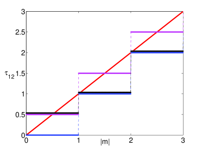
Figure 3: Transition amplitude $\tau_{12}$ as a function of $|m|$ for different methods: quantum without the GP Eq. (35) (blue), quantum with the GP Eq. (40) (black), continuous classical Eq. (41) (red), binned classical Eq. (42) (magenta). $\rho$-dependent parts are neglected in all cases.

However, the solely angular dependence consideration raises a question whether the continuous character of the classical angular momentum will cause overestimation of the transition probability for high $|m|$’s (Fig. 3, ${|m|>1}$). The answer is negative, and it becomes obvious if we account for the $\rho$-dependence of $\tau_{12}$ terms. Although $\rho$ and $L_{z}$ are independent, intuitively, it is clear that for a general trajectory, due to the centrifugal force, high $m$’s have low $1/\rho^{2}$ factors in Eq. (42). Therefore, we can approximate ${(m+1/2)/\rho^{2}\sim m/\rho^{2}}$ for large $|m|$’s. To confirm this intuitive consideration we performed both classical and quantum simulations for the Mexican hat model. In quantum simulations the initial state is given by a Gaussian wave packet placed on the upper cone

$$\chi_{2}(x,y,0)=\sqrt{\frac{2}{\pi\sigma_{x}\sigma_{y}}}\exp{\left(-\frac{(x-x_{0})^{2}}{\sigma_{x}^{2}}-\frac{y^{2}}{\sigma_{y}^{2}}\right)}$$ (43)

with widths $\sigma_{x}=\sigma_{y}=\sqrt{2}$. The classical counterpart is initiated from a Gaussian distribution for positions and momenta obtained via the Wigner transform of $\chi_{2}(x,y,0)$. Average transition amplitudes split to $m$ components in Fig. 4 confirm the conjecture of the radial component ($1/\rho^{2}$) reduction with increase of the angular component ($m$). Moreover, these effects compensate each other consistently through the $m$ series so that both methods plateaux at large $|m|$’s. Therefore, a continuous character of classical angular momentum helps to mimic the enhancement of the fully cylindrical $m=0$ component and does not interfere with other angular components.

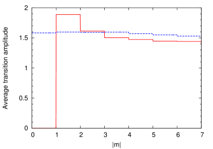
Figure 4: Transition amplitudes, $\hbar^{2}|m\bra{f_{1}}(2\rho)^{-2}\ket{f_{2}}|$ for quantum (sold red) and $\hbar(|m|+1/2)(2\rho)^{-2}$ for MQC (dashed blue) simulations, averaged over the first a.u. of simulation time as a function of $|m|$.

III Molecular calculations

Here we consider three molecular systems: the bis(methylene) adamantyl cation, (BMA)Blancafort, Hunt, and Robb (2005); Izmaylov et al. (2011) the butatriene cation,Köppel, Domcke, and Cederbaum (1984); Cederbaum et al. (1977); Cattarius et al. (2001); Sardar et al. (2008); Burghardt, Gindensperger, and Cederbaum (2006); Gindensperger, Burghardt, and Cederbaum (2006) and the pyrazine molecule.Seidner, Domcke, and von Niessen (1993); Woywod et al. (1994); Sukharev and Seideman (2005) These systems have been extensively studied before, and it was shown that they are well described by multi-dimensional LVC models. For our simulations, we have reduced N-dimensional LVC models to effective 2D LVC models using collective nuclear DOF so that the 2D models reproduce short-term dynamics of the original N-dimensional models [see the Appendix of Ref. Ryabinkin, Joubert-Doriol, and Izmaylov, 2014 for details]. These three systems have LVC parameters (Table 1) that are representative for various manifestations of GP effects.Ryabinkin, Joubert-Doriol, and Izmaylov (2014)

Table 1: Parameters of the 2D effective LVC Hamiltonian, Eq. (2) for the three studied systems.

$\omega_{1}$	$\omega_{2}$	$a$	$c$	$\Delta$	$\gamma$
Bis(methylene) adamantyl cation
$7.743\times 10^{-3}$	$6.680\times 10^{-3}$	31.05	$8.092\times 10^{-5}$	0.000	0.09
Butatriene cation
$9.557\times 10^{-3}$	$3.3515\times 10^{-3}$	20.07	$6.127\times 10^{-4}$	0.020	0.67
Pyrazine
$3.650\times 10^{-3}$	$4.186\times 10^{-3}$	48.45	$4.946\times 10^{-4}$	0.028	1.50

To provide comparative analysis of dynamical features appearing from DBOC and GP influences in addition to MQC simulations we provide quantum results obtained using three nuclear non-adiabatic Hamiltonians: 1) the full Hamiltonian [Eq. (2)] producing exact dynamics, 2) the “no GP” Hamiltonian [Eqs. (8), (12), and (13)], and 3) the “no GP, no DBOC” Hamiltonian [Eqs. (8), (13), and $\tau_{ii}=0$]. Numerical procedures to propagate the TDSE with these Hamiltonians are detailed in Ref. Ryabinkin, Joubert-Doriol, and Izmaylov, 2014. For all methods we compare the adiabatic population of the excited electronic state $P_{\rm adi}^{(e)}(t)=\braket{\chi_{2}(t)}{\chi_{2}(t)}$, where $\chi_{2}(x,y,t)$ is a time-dependent nuclear wave-function that corresponds to the excited adiabatic electronic state initiated as a Gaussian distribution in Eq. (43) with widths $\sigma_{x}=\sqrt{2/\omega_{1}}$ and $\sigma_{y}=\sqrt{2/\omega_{2}}$. To calculate $P_{\rm adi}^{(e)}(t)$ in MQC simulations, $|c_{2}|^{2}(t)$ are used in the EF approach, and the instantaneous ratios between the number of trajectories on the excited state to the total number of trajectories are taken in the SH approach. In both MQC methods, $P_{\rm adi}^{(e)}(t)$ are averaged over 2000 trajectories with nuclear momenta and positions sampled from the Wigner transform of the corresponding quantum wave packet. To integrate MQC EOM, the 4th order Runge-Kutta integrator has been used with the time-step 0.05 fs for SH and 0.001 fs for EF methods, respectively. For the SH method we used Tully’s fewest switches algorithmTully (1990) with nuclear forces obtained from adiabatic PESs, $W_{i}$ [Eq. (9)]. To illustrate the influence of the DBOC in SH dynamics, we introduce a modification, further referred as SH+DBOC, where nuclear forces are obtained from adiabatic PESs with the DBOC, $\tilde{W}_{i}$ [Eq. (27)].

As has been established in our previous study,Ryabinkin, Joubert-Doriol, and Izmaylov (2014) GP effects manifest themselves quite differently in these molecular models: for BMA, GP effects are predominantly in compensation of a potential repulsion introduced by the DBOC, while for the butatriene cation and the pyrazine molecule the GP enhances non-adiabatic transfer of wave-packet’s $m=0$ component. This difference stems from the anisotropy of the branching space, which is well characterized by the value of $|\gamma-\gamma^{-1}|$, the smaller this value is the closer the problem to the Mexican hat case is and more cylindrical all potential terms including the DBOC are. For BMA, $|\gamma-\gamma^{-1}|=11.4$ and this makes the DBOC a wide repulsive wall, while for the other systems, $|\gamma-\gamma^{-1}|\sim 0.8$ which is much closer to the Mexican hat limit ($|\gamma-\gamma^{-1}|=0$). Thus, we will initially analyze performance of the MQC methods for the BMA cation and then for the other two systems.

BMA: DBOC in MQC.

The exact population dynamics in BMA demonstrates coherent oscillations that can be easily understood considering weak diabatic couplings in this system (Fig. 5). Thus, the exact dynamics almost solely undergoes on a single diabatic state that corresponds to the excited adiabatic state before the crossing and the ground adiabatic state after the crossing. Excited state populations in both MQC methods reproduce almost exactly those of the full QM dynamics. Smaller amplitudes of adiabatic population oscillations in SH than those in the exact dynamics is a manifestation of SH overestimation of diabatic population transfer. The origin of this overestimation and violation of the Marcus theory limit has been found in higher electronic coherences within the SH approach.Landry and Subotnik (2011, 2012) The explanation of the overall success of the MQC methods for BMA is in the absence of both GP and DBOC terms in these methods. Therefore the MQC methods do not need the GP for cases where the main role of the GP is the DBOC compensation. On the other hand, comparing the SH+DBOC dynamics with the exact one shows that adding the DBOC to the adiabatic potentials can be very detrimental for MQC results (Fig. 5). The impact of uncompensated DBOC terms in MQC dynamics is even bigger than removing GP terms in quantum simulations. This is a result of a repulsive potential of the DBOC that prevents classical nuclear dynamics in the SH method to approach a region of strong non-adiabatic coupling. Quantum wave packets for the “no GP” Hamiltonian can increase the non-adiabatic transfer due to some tunnelling under the DBOC potential. Thus these results demonstrate that the DBOC should not be added to the MQC methods.

Although the BMA branching space is significantly anisotropic, the transfer of the wave-packet $m=0$ component is still somewhat suppressed.Ryabinkin, Joubert-Doriol, and Izmaylov (2014) Since the weight of the wave-packet $m=0$ component near the CI for BMA is quite substantial, 42%, absence of the GP enhancement of its transition in the “no DBOC, no GP” model results in deviation of the corresponding population dynamics from the exact one after 4 fs. Thus, even in anisotropic systems the GP induced non-adiabatic transfer enhancement and its imitation by MQC methods can be crucial for quantitative agreement with exact dynamics.

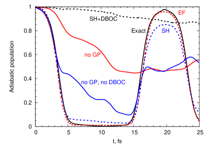
Figure 5: Excited state adiabatic population ($P_{\rm adi}^{(e)}$) dynamics for the BMA cation obtained with different methods.

C₄H${}_{4}^{+}$ and pyrazine: $m=0$ enhancement in MQC.

In the butatriene cation and the pyrazine molecule, the DBOC potential is relatively isotropic and compact. Therefore, it does not prevent a nuclear wave packet from accessing the vicinity of the CI, and the DBOC presence does not change quantum dynamics significantly (see Figs. 6 and 7). Yet, GP effects are significant, because the GP related term in $\tau_{12}^{\rm GP}$ accelerates the non-adiabatic transfer for the $m=0$ component. Interestingly, this acceleration is well mimicked by the MQC methods due to the classical description of the angular momentum which leads to similar enhancement of the $m=0$ component transfer. According to the angular decomposition of quantum wave packets at the moment of the closest proximity to the CI, in both systems, the weight of the $m=0$ component is close to 90%. Therefore, this enhancement is the main GP effect in these systems. The excited state population dynamics in Figs. 6 and 7 reveal that the MQC methods can reproduce the exact quantum dynamics and perform better than quantum methods that do not account for the GP. In both systems, the SH method performs slightly better compared to the EF approach.

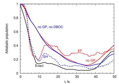
Figure 6: Excited state adiabatic population ($P_{\rm adi}^{(e)}$) dynamics of the butatriene cation obtained with different methods.

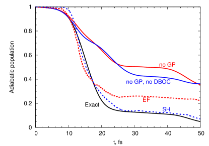
Figure 7: Excited state adiabatic population ($P_{\rm adi}^{(e)}$) dynamics of pyrazine obtained with different methods.

IV Conclusions

It has been recently found that pure quantum effects associated with the nontrivial geometric phase appearing in the nuclear and electronic adiabatic wave-functions for surface crossing problems can significantly affect population transfer dynamics. Although MQC methods ignore nuclear GP effects by substituting quantum nuclear dynamics with its classical approximation, they are still very successful in simulating non-adiabatic dynamics through CIs. In this work we have unraveled the key elements of this success: Both types of GP effects involved in the excited state dynamics, the DBOC compensation and the enhancement of the non-adiabatic transfer for the fully cylindrical component of a wave-packet, are mimicked fortuitously in MQC methods using classical mechanics.

Interestingly, the DBOC term did not appear in original derivations of MQC schemes and have been added only later in an ad hoc manner. This work clearly demonstrated that such addition can be very detrimental for the quality of results and should be avoided. The mechanism for the cylindrical component enhancement in the MQC schemes has been elaborated on the Mexican hat model. The situation in some sense is opposite to the famous Planck quantization via discrete summation to describe the black-body radiation. In MQC transfer element, the purely quantum effect from the GP is recovered because a discrete summation over the angular eigenstates of the angular momentum operator is substituted by a classical continuous integration. Thus, nuclear GP effects make excited state non-adiabatic dynamics more classical by compensating some other quantum effects.

There have been several proposals on using the Landau-Zener (LZ) formulaLandau (1932); Zener (1932) to model non-adiabatic dynamics through the conical intersection.Teller (1937); Alijah and Nikitin (1999); Belyaev, Lasser, and Trigila (2014); Malhado and Hynes (2008) These proposals involve application of the LZ equation for probability transfer with a subsequent averaging over individual classical trajectories. Surprisingly, a question of influence of the conical intersection topology on the result has not ever been raised. The current work can be used to rationalize an application of LZ-based approaches to the CI problem even though in such methods topological geometric phase effects are not explicitly accounted.

V Acknowledgements

A.F.I. acknowledges stimulating discussion with John Tully and funding from the Natural Sciences and Engineering Research Council of Canada (NSERC) through the Discovery Grants Program. R.G. is grateful to the Chemistry Department of the University of Toronto for a summer research fellowship for newly admitted graduate students.

References

- Truhlar and Mead (2003) D. G. Truhlar and C. A. Mead, Phys. Rev. A 68, 032501 (2003).
- Migani and Olivucci (2004) A. Migani and M. Olivucci, in Conical Intersection Electronic Structure, Dynamics and Spectroscopy, edited by W. Domcke, D. R. Yarkony, and H. Köppel (World Scientific, New Jersey, 2004) p. 271.
- Schön and Köppel (1995) J. Schön and H. Köppel, J. Chem. Phys. 103, 9292 (1995).
- Ryabinkin and Izmaylov (2013) I. G. Ryabinkin and A. F. Izmaylov, Phys. Rev. Lett. 111, 220406 (2013).
- Baer et al. (1996) R. Baer, D. M. Charutz, R. Kosloff, and M. Baer, J. Chem. Phys. 105, 9141 (1996).
- Ryabinkin, Joubert-Doriol, and Izmaylov (2014) I. G. Ryabinkin, L. Joubert-Doriol, and A. F. Izmaylov, J. Chem. Phys. 140, 214116 (2014).
- Althorpe, Stecher, and Bouakline (2008) S. C. Althorpe, T. Stecher, and F. Bouakline, J. Chem. Phys. 129, 214117 (2008).
- Bouakline (2014) F. Bouakline, Chemical Physics 442, 31 (2014).
- Cederbaum (2004) L. S. Cederbaum, in Conical Intersections, edited by W. Domcke, D. R. Yarkony, and H. Köppel (World Scientific Co., Singapore, 2004) pp. 3–40.
- Berry (1984) M. V. Berry, Proc. R. Soc. A - Math. Phy. 392, 45 (1984).
- Longuet-Higgins et al. (1958) H. C. Longuet-Higgins, U. Opik, M. H. L. Pryce, and R. A. Sack, P. Roy. Soc. A - Math. Phy. 244, 1 (1958).
- Ben-Nun and Martinez (2002) M. Ben-Nun and T. J. Martinez, Adv. Chem. Phys. 121, 439 (2002).
- Joubert-Doriol, Ryabinkin, and Izmaylov (2013) L. Joubert-Doriol, I. G. Ryabinkin, and A. F. Izmaylov, J. Chem. Phys. 139, 234103 (2013).
- Tully (1990) J. C. Tully, J. Chem. Phys. 93, 1061 (1990).
- Tully (1998) J. C. Tully, Faraday Discuss. 110, 419 (1998).
- Note (1) Formally, through the path integral formalism,Krishna (2007) the GP can be introduced into the classical dynamics but it will not change anything because in the classical limit, the GP for a CI problem results in a delta-function potential at the CI point. Therefore, the number of classical trajectories influenced by the GP is negligible.
- Müller and Stock (1997) U. Müller and G. Stock, J. Chem. Phys. 107, 6230 (1997).
- Worth, Hunt, and Robb (2003) G. A. Worth, P. Hunt, and M. A. Robb, J. Phys. Chem. A 107, 621 (2003).
- Barbatti et al. (2007) M. Barbatti, G. Granucci, M. Persico, M. Ruckenbauer, M. Vazdar, M. Eckert-Maksić, and H. Lischka, J. Photoch. and Photobio. A 190, 228 (2007).
- Ryabinkin et al. (2014) I. G. Ryabinkin, C.-Y. Hsieh, R. Kapral, and A. F. Izmaylov, J. Chem. Phys. 140, 084104 (2014).
- Mead and Truhlar (1979) C. A. Mead and D. G. Truhlar, J. Chem. Phys. 70, 2284 (1979).
- Mead and Truhlar (1982) C. A. Mead and D. G. Truhlar, J. Chem. Phys. 77, 6090 (1982).
- Shenvi (2009) N. Shenvi, J. Chem. Phys. 130, 124117 (2009).
- Akimov and Prezhdo (2013) A. V. Akimov and O. V. Prezhdo, J. Chem. Theory Comput. 9, 4959 (2013).
- Blancafort, Hunt, and Robb (2005) L. Blancafort, P. Hunt, and M. A. Robb, J. Am. Chem. Soc. 127, 3391 (2005).
- Izmaylov et al. (2011) A. F. Izmaylov, D. Mendive-Tapia, M. J. Bearpark, M. A. Robb, J. C. Tully, and M. J. Frisch, J. Chem. Phys. 135, 234106 (2011).
- Köppel, Domcke, and Cederbaum (1984) H. Köppel, W. Domcke, and L. S. Cederbaum, “Multimode Molecular Dynamics Beyond the Born-Oppenheimer Approximation,” (John Wiley & Sons, Inc., 1984) Chap. 2, pp. 59–246.
- Cederbaum et al. (1977) L. Cederbaum, W. Domcke, H. Köppel, and W. Von Niessen, Chem. Phys 26, 169 (1977).
- Cattarius et al. (2001) C. Cattarius, G. A. Worth, H.-D. Meyer, and L. S. Cederbaum, J. Chem. Phys. 115, 2088 (2001).
- Sardar et al. (2008) S. Sardar, A. K. Paul, P. Mondal, B. Sarkar, and S. Adhikari, Phys. Chem. Chem. Phys. 10, 6388 (2008).
- Burghardt, Gindensperger, and Cederbaum (2006) I. Burghardt, E. Gindensperger, and L. S. Cederbaum, Mol. Phys. 104, 1081 (2006).
- Gindensperger, Burghardt, and Cederbaum (2006) E. Gindensperger, I. Burghardt, and L. S. Cederbaum, J. Chem. Phys. 124, 144103 (2006).
- Seidner, Domcke, and von Niessen (1993) L. Seidner, W. Domcke, and W. von Niessen, Chem. Phys. Lett. 205, 117 (1993).
- Woywod et al. (1994) C. Woywod, W. Domcke, A. L. Sobolewski, and H.-J. Werner, J. Chem. Phys. 100, 1400 (1994).
- Sukharev and Seideman (2005) M. Sukharev and T. Seideman, Phys. Rev. A 71, 012509 (2005).
- Landry and Subotnik (2011) B. R. Landry and J. E. Subotnik, J. Chem. Phys. 135, 191101 (2011).
- Landry and Subotnik (2012) B. R. Landry and J. E. Subotnik, J. Chem. Phys. 137, 22A513 (2012).
- Landau (1932) L. D. Landau, Phys. Z. Sowjetunion 1, 88 (1932).
- Zener (1932) C. Zener, P. Roy. Soc. A - Math. Phy. 137, 696 (1932).
- Teller (1937) E. Teller, J. Phys. Chem. 41, 109 (1937).
- Alijah and Nikitin (1999) A. Alijah and E. E. Nikitin, Mol. Phys. 96, 1399 (1999).
- Belyaev, Lasser, and Trigila (2014) A. K. Belyaev, C. Lasser, and G. Trigila, J. Chem. Phys. 140, 224108 (2014).
- Malhado and Hynes (2008) J. P. Malhado and J. T. Hynes, Chem. Phys. 347, 39 (2008).
- Krishna (2007) V. Krishna, J. Chem. Phys. 126, 134107 (2007).