Measurement of thermodynamics using gradient flow

Abstract:

We analyze bulk thermodynamics and correlation functions of the energy-momentum tensor in pure Yang-Mills gauge theory using the energy-momentum tensor defined by the gradient flow and small flow time expansion. Our results on thermodynamic observables are consistent with those obtained by the conventional integral method. The analysis of the correlation function of total energy supports the energy conservation. It is also addressed that these analyses with gradient flow require less statistics compared with the previous methods. All these results suggest that the energy-momentum tensor can be successfully defined and observed on the lattice with moderate numerical costs with the gradient flow.

1 Preliminary

In this manuscript, we consider the energy-momentum tensor

$$T_{\mu\nu}.$$

As is well known, the energy-momentum tensor (EMT) is one of the most fundamental quantities in physics. It is fundamental because this operator is related to the symmetry of space-time; the EMT can be defined as the Noether current of translational symmetry, and it also constitutes generators of Poincaré transformation. Moreover, elements of the EMT, energy and momentum densities and stress tensor, are basic quantities in physics. The EMT also appears in various fundamental equations such as Einstein equation and hydrodynamic equations.

However, if one wants to define and analyze the EMT in lattice QCD Monte Carlo simulations, there are highly nontrivial problems. First, the definition of the EMT itself is nontrivial on the lattice, because the lattice regularization explicitly breaks translational symmetry. For example, a naïve definition,

$$T_{\mu\nu}=\frac{1}{g_{0}^{2}}F_{\mu\rho}^{a}F_{\nu\rho}^{a}-\frac{1}{4g_{0}^{2}}\delta_{\mu\nu}F_{\rho\sigma}^{a}F_{\rho\sigma}^{a},$$ (1)

with a choice of discretized definitions for the field strength $F_{\mu\nu}$ on the lattice, does not give the correct EMT even for off-diagonal components in the sense that it does not correspond to the EMT in the continuum limit [1]. Although the EMT on the lattice can be constructed by an adequate linear combination of operators, the renormalization factor of each operators has to be determined non-perturbatively, which requires additional numerical simulations for each lattice parameter [1, 2]. Second, even if one employs a definition of the EMT on the lattice, its measurement is noisy. For example, the calculation of the correlation function of the EMT requires extremely large statistics [3, 2]. The analysis becomes more noisy as the lattice spacing becomes finer. Because of these reasons, there are not many studies which have analyzed the EMT directly on the lattice.

On the other hand, if one were able to deal with the EMT on the lattice in a controllable manner, various interesting analyses would become possible, because the EMT is one of the most fundamental quantities in physics. For example, if we have the correctly normalized EMT operator on the lattice one can calculate thermodynamic quantities, energy density $\varepsilon$ and pressure $P$, at nonzero temperature by directly taking the thermal expectation values of the diagonal components of the EMT as

$$\varepsilon=-\langle T_{00}\rangle,~{}P=\langle T_{ii}\rangle.$$ (2)

The measurement of bulk thermodynamics on the lattice itself can be done without the EMT; the method based on the thermodynamic relations called the integral method [4] is well established. The measurement with simple relations Eq. (2), however, will provide us with more intuitive way to investigate these quantities. Next, the fluctuations and correlation functions of the EMT are also interesting observables. The fluctuation of the total energy of the system $\bar{T}_{00}$, for example, is related to the specific heat per unit volume as [5]

$$\frac{c_{V}}{T^{3}}=\frac{\langle\delta\bar{T}_{00}^{2}\rangle}{VT^{5}}.$$ (3)

This equation suggests a novel way to analyze $c_{V}$ through the measurement of the energy fluctuation, which becomes possible with the correctly normalized EMT operator. More interesting quantities related to the EMT correlators are transport coefficients. Shear viscosity, for example, is related to the correlation function of $T_{12}$ via the Kubo formula as [6]

$$\eta=\frac{1}{TV}\int_{0}^{\infty}dt\langle\bar{T}_{12}(t);\bar{T}_{12}(0)\rangle,$$ (4)

where $\langle O_{1};O_{2}\rangle$ is the Kubo’s canonical correlation and $\bar{O}=\int_{V}d^{3}xO(x)$. The transport coefficients are important quantities to understand dynamical time evolution of relativistic heavy ion collisions [7]. The measurement of transport coefficients with Kubo formula, however, requires real-time correlation function of the EMT, while the lattice simulations can obtain only imaginary time correlators directly [3, 2]. The analytic continuation from imaginary-time functions to real time is needed, which, however, is a nontrivial procedure requiring an accurate measurement of the EMT correlator.

The application of the EMT operator is not limited to the physics of nonzero temperature. For example, with the correctly normalized EMT operator one would be able to measure the energy and momentum distributions in hadrons and flux tube [8] directly on the lattice. The correlation functions of the EMT in vacuum are also a useful probe to understand vacuum structure of the gauge theory.

Recently, a construction of the EMT in gauge theory is proposed in Ref. [9] on the basis of the Yang-Mills gradient flow [10] and the so-called small flow time expansion [11]. In this method, the constructed EMT is renormalized and does not have divergences, and this property is kept even for the lattice regularization. Moreover, the statistical error is expected to be reduced thanks to the cooling nature of the gradient flow. Therefore, this method can become a solution for the longstanding problem on the measurement of the EMT on the lattice. In this manuscript, we report the first numerical analysis of the EMT in this method in lattice simulations [12].

2 Gradient flow

Because we use the Yang-Mills gradient flow to define the EMT, let us first give a brief review on this concept. The gradient flow for the Yang-Mills gauge field is the continuous transformation of the field defined by the differential equation [10]

$$\frac{dA_{\mu}}{dt}=-g_{0}^{2}\frac{\partial S_{\rm YM}(t)}{\partial A_{\mu}}=D_{\nu}G_{\nu\mu},$$ (5)

with the Yang-Mills action $S_{\rm YM}(t)$ composed of $A_{\mu}(t)$. Color indices are suppressed for simplicity. The initial condition at $t=0$ is taken for the field in the conventional gauge theory; $A_{\mu}(0)=A_{\mu}$. The flow time $t$, which has a dimension of inverse mass squared, is a parameter which controls the transformation. The gauge field is transformed along the steepest descent direction as $t$ increases. At the tree level, Eq. (5) is rewritten as

$$\frac{dA_{\mu}}{dt}=\partial_{\nu}\partial_{\nu}A_{\mu}+{\rm(gauge~{}dependent~{}terms)}.$$ (6)

Neglecting the gauge dependent terms, Eq. (6) is the diffusion equation in four-dimensional space. For positive $t$, therefore, the gradient flow acts as the cooling of the gauge field with the smearing radius $\sqrt{8t}$. In Ref. [11], it is rigorously proved that all composite operators composed of $A_{\mu}(t)$ take finite values for $t>0$. This property ensures that observables at $t>0$ are automatically renormalized.

Recently, the gradient flow has been applied for various purposes, such as the scale setting, analysis of the running coupling, measurement of topology, as well as the studies on their properties on the lattice; see reviews in Refs. [13, 14] and references [11, 9, 15, 16, 17, 18]. In the present study, we use the gradient flow to define the EMT operator using the small flow time expansion [11, 9, 15].

3 Small flow time expansion and the EMT

In the present study, we consider the EMT defined by the small flow time expansion [9]. In order to illustrate the concept of small flow time expansion, let us consider a composite operator $\tilde{O}(t,x)$ composed of the field $A_{\mu}(t)$ at positive flow time. The small flow time expansion asserts that in the small $t$ limit this operator can be written by a superposition of operators of the original gauge theory at $t=0$ as

$$\tilde{O}(t,x)\xrightarrow[t\to 0]{}\sum_{i}c_{i}(t)O_{i}^{\rm R}(x),$$ (7)

where $O_{i}^{\rm R}(x)$ on the right-hand side represents renormalized operators in some regularization scheme in the original gauge theory at $t=0$ with the subscript $i$ denoting different operators, and $x$ represents the coordinate in four dimensional space-time.

The relation Eq. (7) is reminiscent of the operator product expansion (OPE). While a product of operators at different space-time points are expanded by local operators in the OPE, Eq. (7) relates an operator at $t>0$ with those of $t=0$. The validity of this expansion is expected from the cooling nature of the gradient flow; since the operator $\tilde{O}(t,x)$ depends on the fundamental gauge theory only inside the smearing radius $\sqrt{8t}$ around $x$, $\tilde{O}(t,x)$ should be described by the local property of the fundamental theory at $x$ in $t\to 0$ limit. Similarly to the Wilson coefficients in the OPE, the coefficients $c_{i}(t)$ in Eq. (7) can be calculated perturbatively [11, 9].

Using Eq. (7), one can define the renormalized EMT [9]. For this purpose, we first consider dimension-four gauge-invariant operators for operators of the left-hand side in Eq. (7). In pure gauge theory, there are two such operators;

$$U_{\mu\nu}(t,x) =G_{\mu\rho}^{a}(t,x)G_{\nu\rho}^{a}(t,x)-\frac{1}{4}\delta_{\mu\nu}G_{\rho\sigma}^{a}(t,x)G_{\rho\sigma}^{a}(t,x),$$ (8)

$$E(t,x) =\frac{1}{4}G_{\mu\nu}^{a}(t,x)G_{\mu\nu}^{a}(t,x).$$ (9)

Although Eqs. (8) and (9) are quite similar to the traceless-part and trace of the EMT, they are not the EMT since $G_{\mu\nu}(t,x)$ is defined at nonzero flow time $t>0$. Because these operators are gauge invariant, when they are expanded as in Eq. (7) only gauge invariant operators can appear in the right-hand side. Such operator with the lowest dimension is an identity operator. In the expansion of the traceless operator Eq. (8), however, the constant term cannot appear. The next gauge-invariant operators are the dimension-four EMTs. Up to this order, therefore, the small flow time expansions of Eqs. (8) and (9) are given by

$$U_{\mu\nu}(t,x) =\alpha_{U}(t)\left[T_{\mu\nu}^{R}(x)-\frac{1}{4}\delta_{\mu\nu}T_{\rho\rho}^{R}(x)\right]+O(t),$$ (10)

$$E(t,x) =\left\langle E(t,x)\right\rangle_{0}+\alpha_{E}(t)T_{\rho\rho}^{R}(x)+O(t),$$ (11)

where $\langle\cdot\rangle_{0}$ is vacuum expectation value and $T_{\mu\nu}^{R}(x)$ is the correctly normalized conserved EMT with its vacuum expectation value subtracted. Abbreviated are the contributions from the operators of dimension $6$ or higher, which are proportional to powers of $t$ because of dimensional reasons, and thus suppressed for small $t$.

Combining relations Eqs. (10) and (11), we have

$$T_{\mu\nu}^{R}(x)=\lim_{t\to 0}\left\{\frac{1}{\alpha_{U}(t)}U_{\mu\nu}(t,x)+\frac{\delta_{\mu\nu}}{4\alpha_{E}(t)}\left[E(t,x)-\left\langle E(t,x)\right\rangle_{0}\right]\right\}.$$ (12)

The coefficients $\alpha_{U}(t)$ and $\alpha_{E}(t)$ are calculated perturbatively in Ref. [9] as

$$\alpha_{U}(t) =\bar{g}(1/\sqrt{8t})^{2}\left[1+2b_{0}\bar{s}_{1}\bar{g}(1/\sqrt{8t})^{2}+O(\bar{g}^{4})\right],$$ (13)

$$\alpha_{E}(t) =\frac{1}{2b_{0}}\left[1+2b_{0}\bar{s}_{2}\bar{g}(1/\sqrt{8t})^{2}+O(\bar{g}^{4})\right].$$ (14)

Here $\bar{g}(q)$ denotes the running gauge coupling in the $\overline{\text{MS}}$ scheme with the choice, $q=1/\sqrt{8t}$, and

$$\bar{s}_{1} =\frac{7}{16}+\frac{1}{2}\gamma_{E}-\ln 2\simeq 0.032960651891,$$ (15)

$$\bar{s}_{2} =\frac{109}{176}-\frac{b_{1}}{2b_{0}^{2}}=\frac{383}{1936}\simeq 0.19783057851,$$ (16)

with $b_{0}=\frac{1}{(4\pi)^{2}}\frac{11}{3}N_{c}$, $b_{1}=\frac{1}{(4\pi)^{4}}\frac{34}{3}N_{c}^{2}$, and $N_{c}=3$. Note that a non-perturbative determination of $\alpha_{U,E}(t)$ is also proposed recently [15, 19].

There are two important observations: (i) The right-hand side of Eq. (12) is independent of the regularization because of its UV finiteness, so that one can take, e.g., the lattice regularization scheme; (ii) since flowed fields at $t>0$ depend on the fundamental fields at $t=0$ in the space-time region of radius $≃\sqrt{8t}$, the statistical noise in calculating the right-hand side of Eq. (12) is suppressed for finite $t$.

4 Numerical procedure on the lattice

The formula Eq. (12) indicates that $T^{R}_{\mu\nu}(x)$ can be obtained by the small $t$ limit of the gauge-invariant local operators defined through the gradient flow. To perform the numerical analysis on the lattice, we take the following steps:

1. Generate gauge configurations at $t=0$ on a space-time lattice with a standard algorithm with the lattice spacing $a$ and the lattice size $N_{s}^{3}\times N_{\tau}$.

2. Solve the gradient flow for each configuration to obtain the flowed link variables for $t>0$.

3. Construct $U_{\mu\nu}(t,x)$ and $E(t,x)$ in terms of the flowed link variables at each $t$.

4. Determine the right hand side of Eq. (12) for each $t$, and measure expectation values and correlation functions of the EMT by regarding the right hand side of Eq. (12) as the EMT.

5. Carry out an extrapolation toward $(a,t)=(0,0)$.

Note that this analysis has to be performed in the fiducial window, $a\ll\sqrt{8t}\ll R$. Here, $R$ is an infrared cutoff scale such as $\Lambda_{\text{QCD}}^{-1}$ or $T^{-1}=N_{\tau}a$ at which the perturbative analysis used in Eq. (12) is violated. The first inequality is necessary to suppress finite $a$ corrections, while the second one is required to suppress non-perturbative corrections and finite volume effects. We will later see that the upper limit of the fiducial window $R$ is given by by $T^{-1}=N_{\tau}a$ for temperatures analyzed in this study.

5 Numerical setup

To demonstrate that Eq. (12) can successfully be used in the measurement of the EMT on the lattice, we consider the $SU(3)$ gauge theory defined on a four-dimensional Euclidean lattice, whose thermodynamics has been extensively studied by the integral method [4, 20, 21, 22]. We consider the Wilson plaquette gauge action under the periodic boundary condition with several different $\beta=6/g_{0}^{2}$ with $g_{0}$ being the bare coupling constant. The gradient flow in the $t$-direction is numerically solved by the Runge–Kutta method. We have checked that the accumulation errors due to the Runge–Kutta method is more than two order smaller than the statistical errors in all analyses.

$N_{\tau}$	6	8	10	$T/T_{c}$
	6.20	6.40	6.56	1.65
$\beta$	6.02	6.20	6.36	1.24
	5.89	6.06	6.20	0.99

Table 1: Values of $\beta$ and $N_{\tau}$ for each temperature for Setting 1 [12].

$N_{\tau}$	$10$	$12$	$14$	$16$	$20$
$N_{s}$	$64$	$64$	$64$	$64$	$128$
$\beta$	$6.829$	$6.971$	$7.093$	$7.200$	$7.376$

Table 2: Values of $N_{\tau}$, $N_{s}$ and $\beta$ for $T/T_{c}=2.31$ for Setting 2.

The numerical analyses reported in the following have been performed with the following two settings.

• Setting 1: The first analysis is performed on $N_{s}^{3}\times N_{\tau}=32^{3}\times(6,8,10)$ lattices [12]. Gauge configurations are generated by the pseudo-heatbath algorithm with the over-relaxation, mixed in the ratio of $1:5$. We call one pseudo-heatbath update sweep plus five over-relaxation sweeps as a “Sweep”. To eliminate the autocorrelation, we take $200$–$500$ Sweeps between measurements. The number of gauge configurations for the measurements at finite $T$ is $300$. Statistical errors are estimated by the jackknife method. To relate $T/T_{c}$ and corresponding $\beta$ for each $N_{\tau}$, we first use the relation between $a/r_{0}$ ($r_{0}$ is the Sommer scale) and $\beta$ given by the ALPHA Collaboration [23]. The resultant values of $Tr_{0}=[N_{\tau}(a/r_{0})]^{-1}$ are then converted to $T/T_{c}$ by using the result at $\beta=6.20$ in Ref. [4]. Nine combinations of $(N_{\tau},\beta)$ and corresponding $T/T_{c}$ obtained by this procedure are shown in Table 1.

• Setting 2: The second analysis is performed on finer lattices with $N_{s}=64$ and $128$ with several values of $N_{\tau}$. The lattice spacing of each $\beta$ are determined originally [24] by the measurements of $t_{0}$ [10] and $w_{0}$ [25] with the gradient flow, and the simulation is performed for several values of $T/T_{c}$. In this manuscript, we present the result only for $T/T_{c}=2.31$. The parameters $\beta$, $N_{\tau}$ and $N_{s}$ for this $T$ are shown in Table 2. To eliminate the autocorrelation, we take $200$ Sweeps between configurations. The estimate of the statistical error by the jackknife method suggests that the autocorrelation between each configuration is well suppressed. The typical number of gauge configurations for each measurement at finite $T$ is $2000$.

To analyze the EMT with Eq. (12), we measure $G^{a}_{\mu\nu}(t,x)$ written in terms of the clover leaf representation on the lattice. To subtract out the $T=0$ contribution, $\langle E(t,x)\rangle_{0}$, we carry out simulations on a $N_{\tau}=N_{s}$ lattice for each $\beta$. Note that this vacuum subtraction is required only for the measurement of the trace anomaly $\Delta=\varepsilon-3P$, while no subtraction is needed for the measurement of the entropy density $s=(\varepsilon+P)/T$. For $\bar{g}$ in $\alpha_{U}(t)$ and $\alpha_{E}(t)$ given by Eqs. (13) and (14), we use the four-loop running coupling with the scale parameter determined by the ALPHA Collaboration, $\Lambda_{\overline{\text{MS}}}=0.602(48)/r_{0}$ [26]. In the following, we present the numerical results of the thermodynamics for two Settings in Secs. 6 and 7, respectively, and then discuss the correlation function of the EMT in Setting 2 in Sec. 8.

6 Thermodynamics: Setting 1

Figure 1: Flow time dependence of the dimensionless interaction measure (top panel) and the dimensionless entropy density (bottom panel) for different lattice spacings at fixed $T/T_{c}=1.65$ [12]. The circles (red) the squares (blue), and the diamonds (black) correspond to $N_{\tau}=6$, $8$, and $10$, respectively. The bold error bars denote the statistical errors, while the thin error bars (brown, cyan, and magenta) include both statistical and systematic errors.

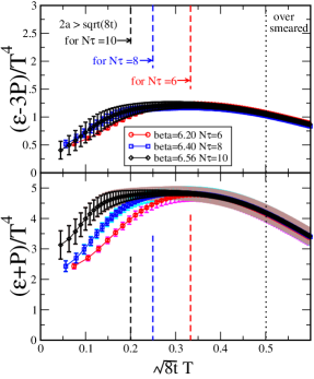
In this section, we first present the numerical results on bulk thermodynamics obtained by the Setting 1 [12]. In Fig. 1, we show the results for the dimensionless trace anomaly $\Delta/T^{4}=(\varepsilon-3P)/T^{4}$ and the dimensionless entropy density $s/T^{3}=(\varepsilon+P)/T^{4}$ at $T=1.65T_{c}$ as a function of the dimensionless flow parameter $\sqrt{8t}T$ [12]. The bold bars denote the statistical errors, while the thin (light color) bars show the statistical and systematic errors including the uncertainty of $\Lambda_{\overline{\text{MS}}}$. We found that the statistical error is dominant in the small $t$ region for both $\Delta/T^{4}$ and $s/T^{3}$, while the systematic error originating from the scale parameter becomes significant for $s/T^{3}$ in the large $t$ region.

The fiducial window discussed in Sec. 4 is indicated by the dashed lines in Fig. 1. The lower limit of the window, beyond which the lattice discretization error grows, is set to be $\sqrt{8t_{\rm min}}=2a$, where we take into account the fact that our clover leaf operator extends the size $2a$. The upper limit of the window, beyond which the smearing by the gradient flow exceeds the temporal lattice size, is set to be $\sqrt{8t_{\rm max}}=1/(2T)=N_{\tau}a/2$.

The data in Fig. 1 show, within the error bars, that (i) the plateau appears inside the preset fiducial window ($2/N_{\tau}<\sqrt{8t}T<1/2$) for each $N_{\tau}$, and (ii) the plateau extends to the smaller $t$ region as $N_{\tau}$ increases or equivalently as $a$ decreases. It should be remarked that only $300$ gauge configurations are necessary to obtain these results. Similar plateaues as in Fig. 1 also appear inside the fiducial window for other temperatures, $T/T_{c}=1.24$ and $0.99$, with comparable error bars. These features imply that the double extrapolation $(a,t)\to(0,0)$ is indeed possible.

Figure 2: Left: Continuum extrapolation of the thermodynamic quantities for $T/T_{c}=1.65$, $1.24$, and $0.99$. Solid lines and dashed lines correspond to the three-point linear fit and two-point constant fit as a function of $1/N_{\tau}^{2}$, respectively. Extrapolated values of the former (latter) are shown at $1/N_{\tau}^{2}=0$ ($1/N_{\tau}^{2}=-0.001$). The cross symbols in the top panel are the data of Ref. [4] with the same lattice setup. Right: Continuum limit of the interaction measure and entropy density obtained by the gradient flow for $T/T_{c}=1.65$, $1.24$, and $0.99$ with $300$ gauge configurations. The results obtained by the integral method in Refs. [4], [20] and [22] are also plotted.

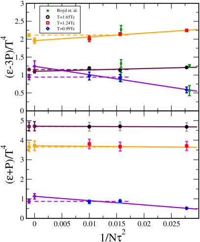
Our lattice results at fixed $T$ with three different lattice spacings allow us to take the continuum limit. First, we pick up a flow time $\sqrt{8t}T=0.40$ which is in the middle of the fiducial window. Then we extract $\Delta/T^{4}$ and $s/T^{3}$ for each set of $N_{\tau}$ and $\beta$. In the left panel of Fig. 2, resultant values taking into account the statistical errors (bold error bars) and the statistical plus systematic errors (thin error bars) are shown. The lattice data for $\Delta/T^{4}$ with the same lattice setup at $N_{\tau}=6$ and $8$ in Ref. [4] are also shown by the cross (green) symbols in the top panel; our results with $300$ gauge configurations have substantially smaller error bars at these points.

Figure 3: Continuum extrapolation in Setting 1 (a) and Setting 2 (b).

We note that the continuum extrapolation in this analysis [12] is taken with fixed $t$; this procedure is graphically shown in Fig. 3 (a). Strictly speaking, however, the double limit $(a,t)\to(0,0)$ has to be taken as mentioned above. Although we have checked that different choices of $t$ do not change the final results within the error bar as long as it is in the plateau region in the analysis in Setting 1, in the next section we will see that the limit with fixed $t$ shows a deviation compared with the double limit when the statistics is improved.

The horizontal axis of the left panel of Fig. 2, $1/N_{\tau}^{2}$, is a variable suited for making continuum extrapolation of the thermodynamic quantities [4]. We consider two ways of extrapolation: A linear fit with the data at $N_{\tau}=6$, $8$, and $10$ (the solid lines in the left panel of Fig. 2), and a constant fit with the data at $N_{\tau}=8$ and $10$ (the dashed lines in the left panel of Fig. 2). In both fits, the correlation between the errors due to the common systematic error from $\Lambda_{\overline{\text{MS}}}$ is taken into account. The former fit is used to determine the central value in the continuum limit whose error is within $\pm 12\%$ even at our lowest temperature. The latter is used to estimate the systematic error from the scaling violation whose typical size is $\pm 4\%$ at high temperature and $\pm 24\%$ at low temperature.

We have analyzed various systematic errors; the perturbative expansion of $\alpha_{U,E}(t)$, the running coupling $\bar{g}$, the scale parameter, and the continuum extrapolation. We found that the dominant errors in the present lattice setup are those from $\Lambda_{\overline{\text{MS}}}$ and the continuum extrapolation, which are included in the left panel of Fig. 2. To reduce these systematic errors, finer lattices are quite helpful: They make the plateau in $\sqrt{8t}T$ wider by reducing the lower limit of the fiducial window, so that the continuum extrapolation becomes easier. Also, larger aspect ratio $N_{s}/N_{\tau}$ would be helpful to guarantee the thermodynamic limit.

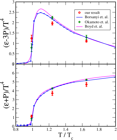
Finally, we plot, in the right panel of Fig. 2, the continuum limit of $\Delta/T^{4}$ and $s/T^{3}$ obtained by the linear fit of the $N_{\tau}=6$, $8$, and $10$ data (the solid lines) in the left panel of Fig. 2 for $T/T_{c}=1.65$, $1.24$, and $0.99$. For comparison to the existing data of the $SU(3)$ gauge theory after the continuum extrapolation, the results of Refs. [4] [20] and [22] obtained by the integral method are also plotted in the right panel of Fig. 2. The results of the two different approaches are consistent with each other within $2$ sigma level. The figure, however, indicates that our results underestimate the observables compared with the previous ones. This discrepancy in part come from the continuum extrapolation with fixed $t$. The correct double limit will be discussed in the next section.

7 Thermodynamics: Setting 2

Figure 4: Flow time dependence of the dimensionless entropy density $s=(\varepsilon+P)/T$ at $T/T_{c}=2.31$ for several values of $N_{\tau}$ with $N_{s}=64$ and $128$. The same result is plotted as functions of $\sqrt{8t}T$ (left panel) and $tT^{2}$ (right panel). The errorbars denote statistical error.

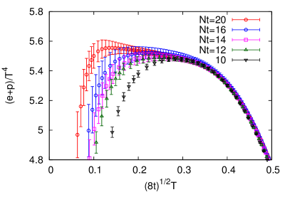
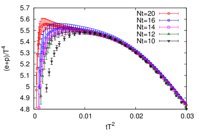
Next, let us see the numerical results on thermodynamics with finer lattices with Setting 2. In the left panel of Fig. 4, we show the dimensionless entropy density $s/T^{3}=(\varepsilon+P)/T^{4}$ as a function of $\sqrt{8t}T$ for $T/T_{c}=2.31$ with $N_{s}=64$ and $128$ for several values of $N_{\tau}$. In this result, one can take a closer look at the $t$ dependence of $s/T^{3}$ thanks to the improved statistics and finer lattices. In the previous section, we discussed that a plateau is observed in the fiducial window, $2a<\sqrt{8t}<1/T$, in Setting 1. Because the statistics is significantly improved in Setting 2, in Fig. 4 one sees a $t$ dependent structure in the fiducial window with $N_{t}=10$. Next, while the $t$ dependence at small $t$ becomes more stable as the lattice spacing becomes finer, the $t$ dependence does not show a plateau even on the finest lattice with $N_{\tau}=20$. In the right panel of Fig. 4, the same result is shown as a function of $tT^{2}$ instead of $\sqrt{8t}T$. The figure indicates that $s/T^{3}$ behaves as a linear function of $t$ as the lattice spacing becomes finer.

The origin of the linear term can be understood as the contribution of higher dimensional operators in Eq. (12) giving rise to $O(t)$ contribution to this formula. In fact, the contribution of dimension six operators are proportional to $t$ in $t\to 0$ limit. Figure 4 shows that the effect of these terms has nonnegligible contribution. Such a contribution has to be subtracted to measure thermodynamic quantities. A similar result is obtained for $\Delta/T^{4}$, while the $t$ dependence is weaker than the one in $s/T^{3}$.

The $O(t)$ effect discussed here can be eliminated by taking the double limit $(a,t)\to(0,0)$. In order to take this double extrapolation, in this analysis we take $a\to 0$ limit with fixed $t/a^{2}$; this procedure is graphically shown in Fig. 3 (b). Here, the ratio $t/a^{2}$ has to be sufficiently large so that $t$ and $a$ satisfy the condition $2a<\sqrt{8t}$, or $t/a^{2}>1/2$. Once this condition is satisfied, however, the double limit can be taken safely irrespective of the value of $t/a^{2}$. In this extrapolation, it is expected that the discretization effect is of order $a^{2}$. This is because the leading discretization error on thermodynamic observables is order $a^{2}$ [4], while the error arising from nonzero $t$ is of order $t$.

Figure 5: Continuum extrapolation of $s$ and $\Delta$. Double extrapolation $(a,t)\to(0,0)$ is taken by taking $a\to 0$ limit with fixed $t/a^{2}=1.0$ and $1.3$.

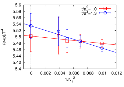
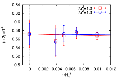
In Fig. 5, we show the result of the continuum extrapolation for $s/T^{3}$ and $\Delta/T^{4}$ with fixed $t/a^{2}$ for $t/a^{2}=1$ and $1.3$. We choose $1/N_{\tau}^{2}$ for the horizontal axis and take a linear extrapolation because of the $a$ dependence discussed above. The result shows that the continuum extrapolation is stable and the extrapolations with different $t/a^{2}$ are consistent. Because of the negative slope in Fig. 4, the continuum extrapolation of $s/T^{3}$ obtained in this method gives slightly larger value compared with the result in the previous section. The final results after the double extrapolation are consistent with the existing results in the integral method [4, 22].

8 Correlation function

Figure 6: Imaginary time correlation function of the total energy, $C_{E}(\tau)/T^{5}=\langle\delta\bar{T}_{00}(\tau)\delta\bar{T}_{00}(0)\rangle/(VT^{5})$, for several values of $t/a^{2}$ for $T/T_{c}=2.31$ obtained on $64^{3}\times 16$ lattice.

Once the operator of the EMT on the lattice is obtained, the application of this operator is not limited to the bulk thermodynamics which is given by expectation values of one point functions. In this section, as an example of other applications we consider the correlation function of the EMT. As discussed in Sec. 1, the correlation functions of the EMT are important observables related to transport properties of the medium and fluctuations.

In this manuscript, as an example of such analyses we present the numerical result on the Euclidean correlation function of the total energy,

$$C_{E}(\tau)=\frac{1}{V}\langle\delta\bar{T}_{00}(\tau)\delta\bar{T}_{00}(0)\rangle,$$ (17)

with $\bar{T}_{00}=\int d^{3}xT_{00}(x,\tau)$ and $\delta\bar{T}_{00}=\bar{T}_{00}-\langle\bar{T}_{00}\rangle$

When one investigates correlation functions of the EMT with Eq. (12), one has to take care of the cooling nature of the gradient flow. When correlation functions are observed on this field, the smearing nature gives rise to artificial correlations in two point correlators when the two operators are not separated twice the smearing length. Because of Eq. (6), the smearing radius defined by the mean square distance in four dimensional space is $\sqrt{8t}$ [10]. When one focuses on a smearing along one definite direction, on the other hand, the smearing length is $\sqrt{2t}$. Therefore, the correlation function Eq. (17) receives an artificial effect due to the smearing for $\tau\lesssim 2\sqrt{2t}$.

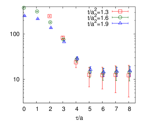
Keeping this precaution in mind, let us see the numerical result on Eq. (17). In Fig. 6, we show $\tau$ dependence of the correlator Eq. (17) for several values of the flow time $t$ for $T/T_{c}=2.31$ and $N_{\tau}=16$. From the figure, one can see several interesting features. First, $C_{E}(\tau)$ takes a large value for $\tau\lesssim 2\sqrt{2t}$ in which the above-mentioned smearing problem affects the correlation function. The enhancement of $C_{E}(\tau)$ at $\tau\lesssim 2\sqrt{2t}$ has a clear $t$ dependence, which indicates that this enhancement is indeed the artificial behavior arising from the gradient flow. On the other hand, the correlator for $\tau\gtrsim 2\sqrt{2t}$ does not have a statistically significant $t$ dependence. This result implies that the correlation function can be obtained in this range. Second, the errorbars of the result are more suppressed for larger $t$. For $t/a^{2}=1.9$, the error is less than $10\%$ with $2000$ configurations. Compared with the previous studies on the EMT correlators [3, 2], this number of statistics is significantly small.

Figure 6 also shows that the correlator Eq. (17) takes a constant within statistics in the range $\tau\gtrsim 2\sqrt{2t}$ at which the smearing effect is well suppressed. This result can be understood as a consequence of the energy conservation, because the energy conservation requires

$$\frac{\partial}{\partial\tau}C_{E}(\tau)=\langle\frac{\partial}{\partial\tau}\bar{T}_{00}(\tau)\bar{T}_{00}(0)\rangle=0,$$ (18)

for $\tau\neq 0$. The emergence of a plateau in Fig. 6, therefore, shows that the EMT defined in Eq. (12) satisfies the energy conservation.

The constant of $C_{E}(\tau)$ gives the thermal fluctuation of the total energy in grand canonical ensemble, i.e.

$$\frac{\langle\delta\bar{T}_{00}^{2}\rangle}{V}=C_{E}(\tau),$$ (19)

where the value of $\tau$ in this formula must satisfy $\tau\gtrsim 2\sqrt{2t}$ in order to avoid the smearing problem. In the continuum theory the value of $\tau$ in Eq. (19) is arbitrary except for $\tau=0$ because of Eq. (18).

Combining Eq. (19) with the linear-response relation Eq. (3), one can make an estimate of the specific heat by reading the value of $C_{E}(\tau)$ in the plateau region in Fig. 6. Here, we use the value of $C_{E}(\tau)$ at midpoint $\tau=\beta/2$. The specific heat is then obtained as

$$c_{V}/T^{3}=15.3(36)\quad{\rm for}\quad T/T_{c}=2.31.$$ (20)

In the analysis of the specific heat of the $SU(3)$ gauge theory in Ref. [27] using the differential method, the values are estimated as $c_{V}/T^{3}=15(1)$ for $T/T_{c}=2$ and $c_{V}/T^{3}=18(2)$ for $T/T_{c}=3$. Although we have not taken the continuum extrapolation, it is notable that our result in Eq. (20) is consistent with the one in Ref. [27]. This result opens a possibility to measure the specific heat in a novel method using the linear-response relation Eq. (3).

9 Summary and outlook

In this study, we analyzed the expectation values and correlation functions of the energy-momentum tensor (EMT) on the lattice using the EMT operator Eq. (12) defined by the gradient flow and the small flow time expansion. Our results show that the numerical analyses of the EMT on the lattice with Eq. (12) work quite successfully. In fact, the thermodynamics observables analyzed in our approach agree with the previous results using integral method. Besides, the result on the energy-energy correlator is consistent with the conservation law and the linear-response relation Eq. (3). Moreover, our approach can perform these measurements with a significantly small statistics compared with the previous methods.

As discussed at the beginning of this manuscript, the measurement of the EMT on the lattice has been a difficult subject, although the EMT is one of the most fundamental quantities in physics. Since the EMT defined by Eq. (12) can become a solution of this longstanding problem, there are a lot of applications of the present study. Among them, the accurate measurement of the correlation functions of the EMT is one of the most interesting subject. While we have only presented the numerical result on the energy-energy correlator in this manuscript, the same analysis can be performed for various channels. In particular, the correlation functions of the spatial components of the EMT, $T_{12}$ and $\sum_{i}T_{ii}$, are interesting because they are related with shear and bulk viscosity, respectively, via Kubo formulas. The measurements of these correlators with Eq. (12) thus would enable us a stable analysis of these quantities on the lattice. Furthermore, the measurements of the energy and momentum distributions in hadrons and flux tube will also be possible using the EMT operator in Eq. (12). These analyses will reveal various aspects of the hadron structure and confinement. The application of this method to full QCD with fermion fields is another important future study [16, 17]. These analyses will be reported elsewhere.

References

- [1] S. Caracciolo, G. Curci, P. Menotti, and A. Pelissetto, The Energy Momentum Tensor for Lattice Gauge Theories, Annals Phys. 197 (1990) 119.
- [2] H. B. Meyer, Transport Properties of the Quark-Gluon Plasma: A Lattice QCD Perspective, Eur.Phys.J. A47 (2011) 86, [arXiv:1104.3708].
- [3] A. Nakamura and S. Sakai, Transport coefficients of gluon plasma, Phys.Rev.Lett. 94 (2005) 072305, [hep-lat/0406009].
- [4] G. Boyd, J. Engels, F. Karsch, E. Laermann, C. Legeland, et al., Thermodynamics of SU(3) lattice gauge theory, Nucl.Phys. B469 (1996) 419–444, [hep-lat/9602007].
- [5] L. D. Landau and E. M. Lifshitz, Statistical Physics. Butterworth-Heinemann, 1980.
- [6] R. Kubo, Statistical Mechanics. North Holland-Amsterdam, 1965.
- [7] P. Romatschke, New Developments in Relativistic Viscous Hydrodynamics, Int.J.Mod.Phys. E19 (2010) 1–53, [arXiv:0902.3663].
- [8] G. Bali, K. Schilling, and C. Schlichter, Observing long color flux tubes in SU(2) lattice gauge theory, Phys.Rev. D51 (1995) 5165–5198, [hep-lat/9409005].
- [9] H. Suzuki, Energy-momentum tensor from the Yang-Mills gradient flow, PTEP 2013 (2013), no. 8 083B03, [arXiv:1304.0533].
- [10] M. Luscher, Properties and uses of the Wilson flow in lattice QCD, JHEP 1008 (2010) 071, [arXiv:1006.4518].
- [11] M. Luscher and P. Weisz, Perturbative analysis of the gradient flow in non-abelian gauge theories, JHEP 1102 (2011) 051, [arXiv:1101.0963].
- [12] FlowQCD Collaboration Collaboration, M. Asakawa, T. Hatsuda, E. Itou, M. Kitazawa, and H. Suzuki, Thermodynamics of SU(3) gauge theory from gradient flow on the lattice, Phys.Rev. D90 (2014), no. 1 011501, [arXiv:1312.7492].
- [13] M. Luscher, Future applications of the Yang-Mills gradient flow in lattice QCD, arXiv:1308.5598.
- [14] A. Ramos, “Wilson flow and renormalization.” this proceedings.
- [15] L. Del Debbio, A. Patella, and A. Rago, Space-time symmetries and the Yang-Mills gradient flow, JHEP 1311 (2013) 212, [arXiv:1306.1173].
- [16] M. Luscher, Chiral symmetry and the Yang–Mills gradient flow, JHEP 1304 (2013) 123, [arXiv:1302.5246].
- [17] H. Makino and H. Suzuki, Lattice energy-momentum tensor from the Yang-Mills gradient flow – inclusion of fermion fields, PTEP 2014 (2014), no. 6 063B02, [arXiv:1403.4772].
- [18] Z. Fodor, K. Holland, J. Kuti, S. Mondal, D. Nogradi, et al., The lattice gradient flow at tree-level and its improvement, JHEP 1409 (2014) 018, [arXiv:1406.0827].
- [19] A. Patella, L. Del Debbio, and A. Rago, Poincare symmetries and the Yang-Mills gradient flow, PoS LATTICE2013 (2014) 324.
- [20] CP-PACS Collaboration Collaboration, M. Okamoto et al., Equation of state for pure SU(3) gauge theory with renormalization group improved action, Phys.Rev. D60 (1999) 094510, [hep-lat/9905005].
- [21] T. Umeda, S. Ejiri, S. Aoki, T. Hatsuda, K. Kanaya, et al., Fixed Scale Approach to Equation of State in Lattice QCD, Phys.Rev. D79 (2009) 051501, [arXiv:0809.2842].
- [22] S. Borsanyi, G. Endrodi, Z. Fodor, S. Katz, and K. Szabo, Precision SU(3) lattice thermodynamics for a large temperature range, JHEP 1207 (2012) 056, [arXiv:1204.6184].
- [23] ALPHA collaboration Collaboration, M. Guagnelli, R. Sommer, and H. Wittig, Precision computation of a low-energy reference scale in quenched lattice QCD, Nucl.Phys. B535 (1998) 389–402, [hep-lat/9806005].
- [24] FlowQCD Collaboration Collaboration, M. Asakawa, T. Hatsuda, T. Iritani, E. Itou, M. Kitazawa, and H. Suzuki. in preparation.
- [25] S. Borsanyi, S. Durr, Z. Fodor, C. Hoelbling, S. D. Katz, et al., High-precision scale setting in lattice QCD, JHEP 1209 (2012) 010, [arXiv:1203.4469].
- [26] ALPHA Collaboration Collaboration, S. Capitani, M. Luscher, R. Sommer, and H. Wittig, Nonperturbative quark mass renormalization in quenched lattice QCD, Nucl.Phys. B544 (1999) 669–698, [hep-lat/9810063].
- [27] R. V. Gavai, S. Gupta, and S. Mukherjee, The Speed of sound and specific heat in the QCD plasma: Hydrodynamics, fluctuations and conformal symmetry, Phys.Rev. D71 (2005) 074013, [hep-lat/0412036].