An Iterative Step-Function Estimator for Graphons

Abstract

Exchangeable graphs arise via a sampling procedure from measurable functions known as graphons. A natural estimation problem is how well we can recover a graphon given a single graph sampled from it. One general framework for estimating a graphon uses step-functions obtained by partitioning the nodes of the graph according to some clustering algorithm. We propose an iterative step-function estimator (ISFE) that, given an initial partition, iteratively clusters nodes based on their edge densities with respect to the previous iteration’s partition. We analyze ISFE and demonstrate its performance in comparison with other graphon estimation techniques.

journalname

, , and

1 Introduction

Latent variable models of graphs can be used to model hidden structure in large networks and have been applied to a variety of problems such as community detection (Girvan and Newman, 2002) and link prediction (Miller et al., 2009). Furthermore, many graphs are naturally modeled as exchangeable when the nodes have no particular ordering (Hoff, 2007). Examples of exchangeable graph models include the stochastic block model (SBM) (Holland et al., 1983) and its extensions (Kemp et al., 2006), latent feature models (Miller et al., 2009; Palla et al., 2012), and latent distance models (Hoff et al., 2002).

Several key inference problems in exchangeable graph models can be formulated in terms of estimating symmetric measurable functions $W\colon[0,1]^{2}\rightarrow[0,1]$, known as graphons. There is a natural sampling procedure that produces an exchangeable (undirected) random graph from a graphon $W$ by first sampling a countably infinite set of independent uniform random variables $\{U_{i}\}_{i\in{{\mathbb{N}}}}$, and then sampling an edge between every pair of distinct vertices $i$ and $j$ according to an independent Bernoulli random variable with weight $W(U_{i},U_{j})$. In the case where the graphon is constant or piecewise constant with a finite number of pieces, this procedure recovers the standard notions of Erdős–Rényi graphs and stochastic block models, respectively. But this procedure is much more general; indeed, Aldous (1981) and Hoover (1979) showed, via what can be viewed as a higher-dimensional analogue of de Finetti’s theorem, that the distribution of any exchangeable graph is some mixture of such sampling procedures from graphons.

Graphon estimation has been studied in two contexts: (1) graphon function estimation (Wolfe and Olhede, 2013; Choi and Wolfe, 2014), where we are concerned with inverting the entire sampling procedure to recover a measurable function from a single sampled graph, and (2) graphon value estimation, where we are interested in inverting just the second step of the sampling procedure, to obtain estimates of the latent values $W(U_{i},U_{j})$ from a single graph (Chatterjee, 2014; Gao et al., 2014) (or several (Airoldi et al., 2013)) sampled using the sequence $\{U_{i}\}_{i\in{{\mathbb{N}}}}$.

Graphons are well-approximated by step-functions in the cut distance (Frieze and Kannan, 1999a, b; Lovász, 2012), a notion of distance between graphs that extends to graphons, which we describe in Section 2. Although the topology on the collection of graphons induced by the cut distance is coarser than that induced by $L^{2}$ (as used in MSE and MISE risk), two graphons are close in the cut distance precisely when their random samples (after reordering) differ by a small fraction of edges. Hence it is natural to consider graphon estimators that produce step-functions; this has been extensively studied with the stochastic block model.

A standard approach to approximating graphons using step-functions is to first partition the vertices of the sampled graph $G$ and then return the step-function graphon determined by the average edge densities in $G$ between classes of the partition. In this way, every clustering algorithm can be seen to induce a graphon estimation procedure (Section 3.2). While many clustering algorithms thereby give rise to tractable graphon estimators, one challenge is to produce clustering algorithms that induce good estimators. In this paper, we introduce a method, motivated by the cut distance, that takes a vertex partition and produces another partition that yields an improved graphon estimate. By iterating this method, even better estimates can be obtained. We describe and analyze the graphon estimator that results from this iterative procedure applied to the result of a clustering algorithm.

1.1 Contributions

We propose iterative step-function estimation (ISFE), a computationally tractable graphon estimation procedure motivated by the goal, suggested by the Frieze–Kannan weak regularity lemma, of finding a partition that induces a step-function estimate close in cut distance to the original graphon. ISFE iteratively improves a partition of the vertices of the sampled graph by considering the average edge densities between each vertex and each of the classes of the existing partition (Section 3).

We analyze a variant of ISFE on graphs sampled from a $2$-step stochastic block model, and demonstrate a sense in which ISFE correctly classifies an arbitrarily large fraction of the vertices, as the number of vertices of the sampled graph and number of classes in the partition increase (Section 4).

Finally, we evaluate our graphon estimation method on data sampled from several graphons, comparing ISFE against several other graphon estimation methods (Section 5). ISFE quickly recovers detailed structure in samples from graphons having block structure, while still performing competitively with other tractable graphon estimators on various classes of continuous graphons, while making fewer structural assumptions.

2 Background and related work

Throughout this paper, graphs are undirected and simple; we consider sequences of graphs that are dense, in that a graph with $n$ vertices has $\Omega(n^{2})$ edges. For natural numbers $n\geq 1$, we define a graph on $[n]$ to be a graph with set of vertices $[n]:=\{1,\ldots,n\}$; its adjacency matrix is the $\{0,1\}$-valued $n\times n$ matrix $(G_{ij})_{i,j\in[n]}$, where $G_{ij}=1$ iff $G$ has an edge between vertices $i$ and $j$. Graphs on ${{\mathbb{N}}}$, and their adjacency matrices, are defined similarly. We write $x\stackrel{{\scriptstyle\mathrm{d}}}{{=}}y$ when two random variables $x$ and $y$ are equal in distribution, and abbreviate almost surely and almost everywhere by a.s. and a.e., respectively.

2.1 Graphons

For detailed background on graphons and the relationship between graphons and exchangeable graphs, see the book by Lovász (2012) and surveys by Diaconis and Janson (2008) and Austin (2008). Here we briefly present the key facts that we will use.

A random graph $G$ on ${{\mathbb{N}}}$ is exchangeable when its distribution is invariant under arbitrary permutations of ${{\mathbb{N}}}$. In particular, if such a graph is not a.s. empty, then the marginal probability of an edge between any two vertices is positive.

Definition 2.1.

A random $\{0,1\}$-valued array $(A_{ij})_{i,j\in{{\mathbb{N}}}}$ is (jointly) exchangeable when

$$(A_{ij})\stackrel{{\scriptstyle\mathrm{d}}}{{=}}(A_{\sigma(i),\sigma(j)})$$ (1)

for every permutation $\sigma$ of ${{\mathbb{N}}}$.

Note that a random graph on ${{\mathbb{N}}}$ is exchangeable precisely when its adjacency matrix is jointly exchangeable. We now define a sampling procedure that produces exchangeable graphs.

Definition 2.2.

A graphon $W$ is a symmetric measurable function $[0,1]^{2}\to[0,1]$.

A graphon can be thought of as a continuum-sized, edge-weighted graph. We can sample from a graphon in the following way.

Definition 2.3.

Let $W$ be a graphon. The $W$-random graph on ${{\mathbb{N}}}$, written $\mathbb{G}({{\mathbb{N}}},W)$, has adjacency matrix $(G_{ij})_{i,j\in{{\mathbb{N}}}}$ given by the following sampling procedure:

$$\begin{split}U_{i}&\stackrel{{\scriptstyle\text{iid}}}{{\sim}}\operatorname{Uniform}[0,1]\\ G_{ij}\ |\ U_{i},U_{j}&\stackrel{{\scriptstyle\text{ind}}}{{\sim}}\operatorname{Bernoulli}(W(U_{i},U_{j}))\textrm{~{}for~{}}i<j\end{split}$$ (2)

For $n\geq 1$, the random graph $\mathbb{G}(n,W)$ on $[n]$ is formed similarly.

Every $W$-random graph is exchangeable, as is any mixture of $W$-random graphs. Conversely, the following statement is implied by the Aldous–Hoover theorem, a two-dimensional generalization of de Finetti’s theorem, which characterizes exchangeable sequences as mixtures of i.i.d. sequences.

Theorem 2.4 (Aldous (1981); Hoover (1979)).

Suppose $G$ is an exchangeable graph on ${{\mathbb{N}}}$. Then $G$ can be written as the mixture of $W$-random graphs $\mathbb{G}({{\mathbb{N}}},W)$ for some probability measure on graphons $W$.

The Aldous–Hoover representation has since been extended to higher dimensions, more general spaces of random variables, and weaker notions of symmetry; for a detailed presentation, see Kallenberg (2005).

Since every exchangeable graph is a mixture of graphon sampling procedures, many network models can be described in this way (Hoff, 2007). The stochastic block model (Holland et al., 1983) is such an example, as explored further by Bickel and Chen (2009) and others; it plays a special role as one of the simplest models that can approximate arbitrary graphon sampling procedures. Some Bayesian nonparametric models, including the eigenmodel (Hoff, 2007), Mondrian process graph model (Roy and Teh, 2008), and random function model (Lloyd et al., 2012) were built knowing the Aldous–Hoover representation. Furthermore, many other such models are naturally expressed in terms of a distribution on graphons (Orbanz and Roy, 2015; Lloyd et al., 2012), including the infinite relational model (IRM) (Kemp et al., 2006) the latent feature relational model (LFRM) (Miller et al., 2009), and the infinite latent attribute model (ILA) (Palla et al., 2012).

Two different graphons $W_{0},W_{1}$ can give rise to the same distribution on graphs, in which case we say that $W_{0}$ and $W_{1}$ are weakly isomorphic. For example, modifying a graphon on a measure zero subset does not change the distribution on graphs. Moreover, applying a measure-preserving transformation to the unit interval, before sampling the graphon, leaves the distribution on graphs unchanged. The following is a consequence of Proposition 7.10 and Equation (10.3) of Lovász (2012).

Proposition 2.5.

Let $\varphi:[0,1]\rightarrow[0,1]$ be a measure-preserving transformation, i.e., a map such that $\varphi(U)$ is uniformly distributed for $U\sim\operatorname{Uniform}[0,1]$. Then the graphon $W^{\varphi}$ defined by $W^{\varphi}(x,y)=W(\varphi(x),\varphi(y))$ is weakly isomorphic to $W$.

Thus, the graphon from which an exchangeable graph is sampled is non-identifiable; see Orbanz and Roy (2015, §III.D). Such measure-preserving transformations are essentially the only freedom allowed. Hence the appropriate object to estimate is a graphon up to weak isomorphism.

Theorem 2.6 (Hoover (1979)).

If $W_{0}$ and $W_{1}$ are weakly isomorphic, then there are measure-preserving transformations $\varphi_{0},\varphi_{1}$ and a graphon $V$ such that $W_{0}^{\varphi_{0}}=W_{1}^{\varphi_{1}}=V$ a.e.

As a result of Theorem 2.6, when considering the problem of estimating a graphon, we only ask to recover the graphon up to a measure-preserving transformation; this is analogous to a key aspect of the definitions of cut distance and of $L^{2}$ distance between graphons, which we describe in Appendix A.

2.2 The graphon estimation problems

Given a graph with adjacency matrix $(G_{ij})$ sampled according to Equation (2), there are two natural ways one may seek to invert this sampling procedure. Here we consider two distinct graphon estimation problems that correspond to inverting one or both of the sampling steps. The “graphon value estimation problem” aims to invert the second step of the sampling procedure, and hence can be thought of as finding the local underlying structure of a graph sampled from a graphon (without concluding anything about the graphon at any location not involved in the sample). Suppose we sample the $W$-random graph $\mathbb{G}(n,W)$ using $\{U_{i}\}_{i\in[n]}$ as in Equation (2). Graphon value estimation consists of giving an estimator $\widehat{M}:=(\widehat{M}_{ij})_{i,j\in[n]}$ for the matrix $M:=(M_{ij})_{i,j\in[n]}$ where each $M_{ij}:=W(U_{i},U_{j})$. One measure of success for the graphon value estimation problem is given by the mean squared error:

$$\operatorname{MSE}(\widehat{M}):=\mathbb{E}\ \Bigl{(}\frac{1}{n^{2}}\sum_{i=1}^{n}\sum_{j=1}^{n}\bigl{(}M_{ij}-\widehat{M}_{ij}\bigr{)}^{2}\Bigr{)},$$ (3)

as used by Chatterjee (2014) and Gao et al. (2014) (see also Airoldi et al. (2013)). Whereas MSE in nonparametric function estimation is typically with respect to particular points of the domain (see, e.g., Tsybakov (2009, §1.2.1)), here the random sequence $\{U_{i}\}_{i\in[n]}$ is latent, and so we take the expectation also with respect to the randomness in the terms $U_{i}$ (and hence in the terms $M_{ij}$), following Chatterjee (2014, §2.6).

The “graphon function estimation problem” aims to invert the entire sampling procedure to recover a graphon (i.e., symmetric measurable function). A notion of success for the graphon function estimator problem, used by Wolfe and Olhede (2013), Choi and Wolfe (2014), and Olhede and Wolfe (2014), is given by the mean integrated squared error for an estimator $\widehat{W}$ of a graphon $W$:

$$\operatorname{MISE}(\widehat{W}) :=\mathbb{E}\ \inf_{\varphi}\ \mathopen{\|}W-\widehat{W}^{\varphi}\mathclose{\|}_{2}$$

$$=\mathbb{E}\ \inf_{\varphi}\int_{[0,1]^{2}}\bigl{(}W(x,y)-\widehat{W}^{\varphi}(x,y)\bigr{)}^{2}\,dx\,dy,$$

where $\varphi$ ranges over measure-preserving transformations of $[0,1]$. However, as we describe in Appendix A.2, there are graphons $W$ and $V$ such that the random graphs $\mathbb{G}({{\mathbb{N}}},W)$ and $\mathbb{G}({{\mathbb{N}}},V)$ are close in distribution, but $W$ and $V$ are far in $L^{2}$ distance. An alternative global notion of success for the function estimation problem is to use the distribution of such random graphs directly (Kallenberg, 1999), or to use the cut distance, defined in terms of the cut along which two graphs differ the most in their edge densities, which also captures this notion of subsamples being close in distribution; see Appendix A.2.

The distinction between these two problems is analogous to the typical distinction between MSE and MISE in nonparametric function estimation (Tsybakov, 2009); see also the two estimation problems in Yang et al. (2014, §2.1).

In general, it is impossible to recover a measurable function from its values at a countable number of points. However, if we assume that the measurable function has specific structure (e.g., is continuous, Lipschitz, a step-function, etc.), then it may become possible. As a result, many graphon estimation methods, which we describe below, require the graphon to have a representation of a certain form. However, the problem of recovering a real-valued function from its values at a random set of inputs, under various assumptions on the function, may be treated separately from the estimation of these values. Hence in this paper, while we illustrate the step-function graphon provided by ISFE, we evaluate its graphon value estimate using MSE.

2.3 Graphon estimation methods

The first study of graphon estimation was by Kallenberg (1999) in the more general context of exchangeable arrays. This work predates the development of the theory of graphons; for details, see Orbanz and Roy (2015, §V).

A number of graphon estimators have been proposed in recent years. Here we mention several that are most closely related to our approach. The stochastic block model approximation (SBA) (Airoldi et al., 2013) requires multiple samples on the same vertex set, but is similar to our approach in some respects, as it partitions the vertex set according to the $L^{2}$ metric on their edge vectors (in essence, the vector of average edge densities with respect to the discrete partition). Sorting and smoothing (SAS) (Chan and Airoldi, 2014) takes a different approach to providing a computational tractable estimator, requiring the graphon to have absolutely continuous degree distribution.

Several estimators use spectral methods, including universal singular value thresholding (USVT) (Chatterjee, 2014). Rather than estimating a specific cluster and using this to define a step-function, Amini and Levina (2014) first estimate a co-cluster matrix and then obtain a graphon estimate from this matrix by using eigenvalue truncation and $k$-means.

Other recent work in graphon estimation has focused on minimax optimality, histogram bin width, estimation using moments, or consequences of the graphon satisfying certain Lipschitz or Hölder conditions (Yang et al., 2014; Wolfe and Olhede, 2013; Olhede and Wolfe, 2014; Bickel and Chen, 2009; Bickel et al., 2011; Choi and Wolfe, 2014).

The estimation problem for latent space models can also be seen as graphon estimation, as such models are equivalent to graphon sampling procedures for graphons having nicer properties than mere measurability (Chatterjee, 2014, §2.4).

Many of the above graphon estimators are formulated in the setting of bipartite graphs and separate exchangeability, where the distribution is invariant under separate permutations of the rows and columns. For notational simplicity, we focus on the case of arbitrary undirected graphs, whose adjacency matrices are symmetric, and for which joint exchangeability is the appropriate notion, but many of our results have straightforward analogues for bipartite graphs.

3 Iterative step-function estimation

We first discuss how a partition of a finite graph’s vertex set induces a step-function graphon and how clustering algorithms produce step-function graphon estimators. Next we propose iterative step-function estimation (ISFE), an approach to iteratively improving such estimates by forming a new partition whose classes contain vertices that have similar edge densities with respect to the old partition.

3.1 Step-function estimators for graphons

A step-function graphon can be associated with any finite graph given a partition of its vertices. Our presentation largely follows §7.1 and §9.2 of Lovász (2012), with modified notation.

A graphon $V$ is called a step-function when there is a partition $\mathcal{S}=\{S_{1},\ldots,S_{k}\}$ of $[0,1]$ into finitely many measurable pieces, called steps, such that $V$ is constant on each set $S_{i}\times S_{j}$. Suppose $H$ is a vertex-weighted, edge-weighted graph on $[n]$, with vertex weights $\alpha_{i}$ and edge-weights $\beta_{ij}$ for $i,j\in[n]$. Then the step-function graphon $W_{H}$ associated with $H$ is defined by $W_{H}(x,y)=\beta_{ij}$ for $x\in J_{i}$ and $y\in J_{j}$, where the steps $J_{1},\ldots,J_{n}$ form a partition of $[0,1]$ into consecutive intervals of size $\frac{\alpha_{i}}{\sum_{j\in[n]}\alpha_{j}}$ for $i\in[n]$. (Consider an unweighted finite graph $G$ to be the weighted graph with vertex weights $\alpha_{i}=1$ and edge weights $\beta_{ij}=G_{ij}$.)

Given a graph $G$ on $[n]$ and vertex sets $X,Y\subseteq[n]$, write $c_{G}(X,Y):=\sum_{i\in X}\sum_{j\in Y}G_{ij}$ for the number of edges across the cut $(X,Y)$. Then the edge density in $G$ between $X$ and $Y$ is defined to be $e_{G}(X,Y):=\dfrac{c_{G}(X,Y)}{|X|\,|Y|};$ when $X$ and $Y$ are disjoint, this quantity is the fraction of possible edges between $X$ and $Y$ that $G$ contains.

Now suppose $G$ is a graph on $[n]$ and $\mathcal{P}=\{P_{1},\ldots,P_{k}\}$ is a partition of the vertices of $G$ into $k$ classes. The quotient graph $G/\mathcal{P}$ is defined to be the weighted graph on $[k]$ with respective vertex weights $|P_{i}|/n$ and edge weights $\frac{e_{G}(P_{i},P_{j})}{|P_{i}|\,|P_{j}|}$. For our estimation procedure, we will routinely pass from a sampled graph $G$ and a partition $\mathcal{P}$ of its vertex set to the graphon $W_{G/\mathcal{P}}$ formed from the quotient $G/\mathcal{P}$.

One may similarly define the step-function graphon $V_{\mathcal{S}}$ of $V$ with respect to a measurable partition $\mathcal{S}=\{S_{1},\ldots,S_{k}\}$ of $[0,1]$ as the step-function graphon of the weighted graph with each vertex weight $\alpha_{i}$ equal to the measure of $S_{i}$ and edge weight $\beta_{ij}=\int_{S_{i}\times S_{j}}V(x,y)\,dx\,dy$.

The Frieze–Kannan weak regularity lemma (Frieze and Kannan, 1999a, b) implies that every graphon is well-approximated in the cut distance by such step-functions formed from measurable partitions; moreover, a bound on the quality of such an approximation is determined by the number of classes in the partition, uniformly in the choice of graphon. For further details, see Appendix A.1.

3.2 Graphon estimation via clustering

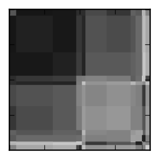
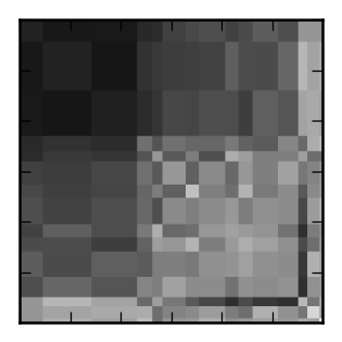
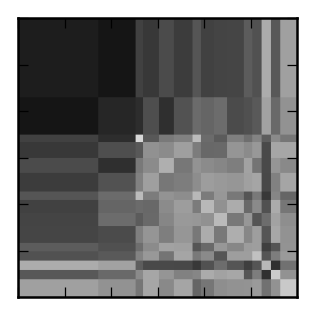
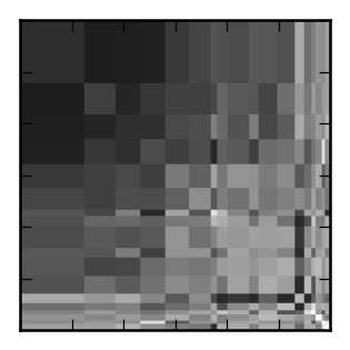
The partition $\mathcal{P}$ of a finite graph $G$ described in Section 3.1, which the step-function $W_{G/\mathcal{P}}$ utilizes, can be formed by clustering the nodes using some general clustering method, such as $k$-means (MacQueen, 1967), hierarchical agglomerative clustering (Ward, Jr., 1963), random assignment, or simpler clusterings, such as the trivial partition, in which all vertices are assigned to a single class, or the discrete partition, in which all vertices are in separate classes.

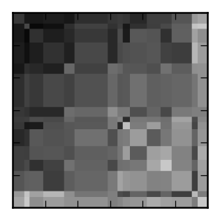
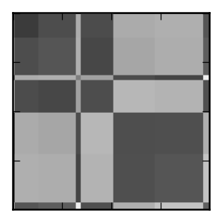
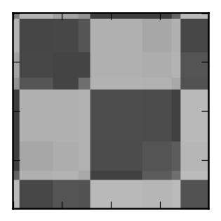
In Figure 1, we display the result of estimating a graphon according to several clustering algorithms. In all graphon figures, we use a grayscale gradient for values on $[0,1]$, where darker values are closer to $1$.

Within the graphon estimator literature, several techniques produce step-functions, but the analysis has generally focused on the choice of partition size (Olhede and Wolfe, 2014) or on the convergence rates for optimal partitions (Wolfe and Olhede, 2013; Choi and Wolfe, 2014; Gao et al., 2014), or else the technique requires multiple observations (Airoldi et al., 2013). Here we aim to exploit structural aspects of graphs, such weak regularity (i.e., their uniform approximability in the cut distance), via an algorithm for forming a new partition that improves the step-function estimate $W_{G/\mathcal{P}}$ produced by any given partition $\mathcal{P}$.

(a) ISFE

(b) $k$-means

(c) Agglomerative

(d) Affinity

(e) Spectral

Figure 1: Comparison of the step-function graphons obtained using various clustering algorithms on an infinite relational model graphon. Columns: (1) ISFE was applied to the trivial partition, where all vertices were initially assigned to a single bin. Clustering was performed using the Python package scikit-learn (Pedregosa et al., 2011) clustering defaults for (2) $k$-means, (3) agglomerative clustering, (4) affinity propagation, and (5) spectral clustering, except that the number of clusters was set to $k=15$ for each method that uses a fixed cluster size.

3.3 Iterative step-function estimation

In Algorithm 1, we describe iterative step-function estimation (ISFE), which can be used to produce graphon function and value estimates.

Given a finite graph $G$, consider the following graphon function estimator procedure: (a) partition the vertices of $G$ according to some clustering algorithm; (b) repeatedly improve this partition by iteratively running Algorithm 1 for $T\geq 0$ iterations; and (c) report the step-function graphon $W_{G/\mathcal{P}}$, where $\mathcal{P}$ is the final partition produced, with its classes sorted according to their average edge densities. Let $V$ be a graphon and $n\in{{\mathbb{N}}}$, and suppose $G$ is a sample of the $V$-random graph $\mathbb{G}(n,V)$. The ISFE procedure on $G$ can be evaluated as a graphon function estimate in terms of MISE by directly comparing $W_{G/\mathcal{P}}$ to $V$.

ISFE can also be used to produce a graphon value estimate from a graph $G$ on $[n]$. Let $k$ be the number of classes in an initial partition $\mathcal{P}$ of $G$. Implicit in the ISFE procedure is a map $p:[n]\to[k]$ sending each vertex of $G$ to the index of its class in $\mathcal{P}$. A graphon value estimate is then given by $\widehat{M}=\bigl{(}W_{G/\mathcal{P}}(\frac{2p(i)-1}{2k},\frac{2p(j)-1}{2k})\bigr{)}_{i,j\in[n]}$. In other words, a regular grid $(\frac{2\ell-1}{2k},\frac{2m-1}{2k})_{\ell,m\in[k]}$ of $k\times k$ points within $[0,1]^{2}$ is chosen as a set of representatives of the piecewise constant regions of $W_{G/\mathcal{P}}$, in some order that corresponds to how the vertices of $G$ were rearranged into the partition $\mathcal{P}$. In a synthetic run, where $G$ is a sample of the $V$-random graph $\mathbb{G}(n,V)$ and we retain the history of how $\mathcal{P}$ was formed from the values $M=\bigl{(}V(U_{i},U_{j})\bigr{)}_{i,j\in[n]}$, MSE can be evaluated by comparing $M$ with $\widehat{M}$.

Input: graph $G$, initial partition $\mathcal{P}^{(\text{old})}$, min. classes $\ell$, decay $d$

Output: new partition $\mathcal{P}^{(\text{new})}$

Initialize $\mathcal{Q}=\{Q_{1}\},Q_{1}=\{1\},c_{1}=1,\epsilon=1$.

while number of classes $|\mathcal{Q}|<\ell$ do

     for vertices $i=2,\ldots,n$ do

         Compute weighted edge-densities vector

            $e_{i}:=\bigl{\{}\frac{|P_{j}|}{n}\,e_{G}(\{i\},P_{j})\bigr{\}}_{j}$ $\text{for }j=1,\ldots,|\mathcal{P}^{(\text{old})}|.$

         Find $j$ minimizing $L^{1}$ distance between vectors $e_{i}$,$e_{c_{j}}$:

            $j^{*}:=\arg\min_{j}d_{j}(e_{i},e_{c_{j}})$, where

            $d_{j}(e_{i},e_{c_{j}}):=\sum_{r}\bigl{|}\frac{|P_{r}|}{n}e_{G}(\{i\},P_{r})-\frac{|P_{r}|}{n}e_{G}(\{c_{j}\},P_{r})\bigr{|}$.

         if minimum distance $d_{j^{*}}(e_{i},e_{c_{j}})<\epsilon$ then

              Add vertex $i$ to existing class $Q_{j^{*}}$.

         else

              Create new class $Q_{B}=\{i\}$, where $B=|\mathcal{Q}|+1$.

              Set centroid $c_{B}=i$.

              Add class $Q_{B}$ to partition $\mathcal{Q}$.               

     Reduce $\epsilon$ by the decay parameter: $\epsilon\leftarrow\epsilon\cdot d$.

Return $\mathcal{P}^{(\text{new})}\leftarrow\mathcal{Q}$.

Algorithm 1 ​​.  Single iteration

(a) $T=0$

(b) $T=1$

(c) $T=2$

(d) $T=3$

(e) $T=4$

Figure 2: The first 4 iterations of ISFE on a 200 vertex sample from a SBM graphon with $p=0.5,q=(0.7,0.3)$, beginning with a random partition into 6 classes $(T=0)$.

As discussed in Section 3.1, by the weak regularity lemma for graphons, every graphon can be approximated to arbitrary accuracy in cut distance by a step-function, whose number of steps depends on the desired accuracy and not the graphon. ISFE seeks to take advantage of this structure. In an iteration of ISFE, each vertex is grouped with other vertices that are similar in average edge density with respect to the input partition, weighted by the size of each class. In this way, ISFE optimizes average edge densities between classes of the partition in proportion to the number of vertices they contain. Each subsequent iteration seeks to improve upon the previous partition, by using it as the basis for the next round of density calculations.

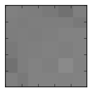
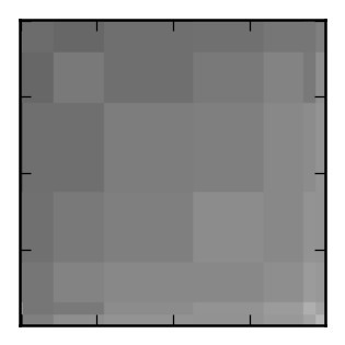
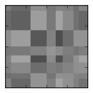
Figure 2 demonstrates how ISFE extracts structure from a graph sampled from an SBM over the course of several iterations, beginning with a random partition ($T=0$), in which each vertex is independently placed into one of 6 classes uniformly at random. (For details on the SBM parameters, see Section 3.4 below.) Slight discrepancies in the edge densities between classes in the random partition of $T=0$ are amplified in iterations $T=1,2$. The substantial correlations between the classes of the partition obtained in $T=2$ and the true block structure allow in $T=3$ to produce a partition each of whose classes is largely from a single block. This is refined slightly in $T=4$.

3.4 Examples of ISFE

We now present examples of the behavior of ISFE on certain classes of graphons. In Appendix B.1, we discuss how ISFE performs on step-functions of finite graphs.

Stochastic block model

The stochastic block model (SBM) has been extensively studied from many perspectives; for a survey of some of the statistical literature as it relates to the graphon estimation problems, see Chatterjee (2014, §2.2).

In the stochastic block model, we assume there is some fixed finite number of classes. We define the SBM graphon with $2$ classes as follows: given parameters $p\in[0,1],q=(q_{0},q_{1})\in[0,1]^{2}$, we partition $[0,1]$ into two pieces $P_{0},P_{1}$ of length $p$ and $1-p$, where $p\in[0,1]$. The value of the graphon is constant on $P_{i}\times P_{i}$ with value $q_{0}$ and constant on $P_{i}\times P_{1-i}$ with value $q_{1}$, for $i=0,1$.

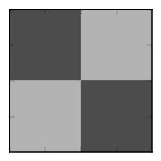
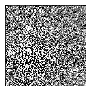
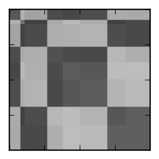
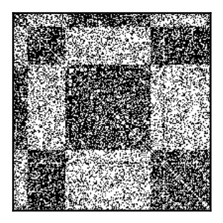
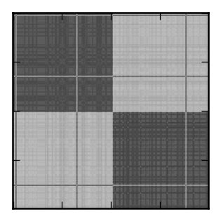
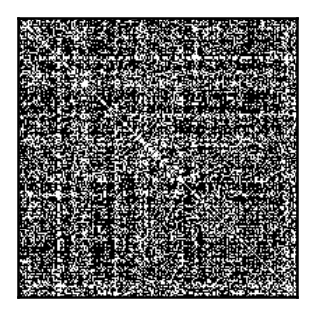
We show the result of ISFE on a graph sampled from an SBM graphon in Figure 3(a) for $p=0.5,q=(0.7,0.3)$. In the first column, we plot the graphon. We sample a 200 vertex graph from this SBM (column 2) and run ISFE (starting with the trivial partition) on the sample with $\ell=8$ for $T=5$ iterations (column 3). We show in the fourth column the original sample rearranged according to the step-function estimate produced by ISFE. The last column is the step-function estimate discretized on a $200\times 200$ grid and sorted according to increasing $U_{i}$ value. (On non-synthetic datasets, where there are no such values $U_{i}$, it is not possible to produce this reordering.) The graphon in this final column is more easily visually compared to the original graphon in column 1, whereas the original estimate in column 3 shows more directly the partition found by ISFE.

(a) Stochastic block model

(b) Infinite relational model

Figure 3: Examples of graphon estimation using ISFE. Rows: (a) an SBM graphon and (b) an IRM graphon. Columns: (1) the original graphon; (2) a 200 vertex random sample from the graphon; (3) ISFE result with $\ell=8$ (SBM), $15$ (IRM), $T=4$ on a 200-vertex sample; (4) the random sample reordered according to the ISFE estimate; (5) ISFE estimate rearranged by increasing $U_{i}$. ISFE was applied to the trivial partition, i.e., all vertices were initially in a single class.

Infinite relational model

The infinite relational model (IRM) (Kemp et al., 2006) is a non-parametric extension of the SBM, where the (infinite) partition is generated by a Chinese restaurant process with concentration parameter $\alpha$. For a description of the distribution on graphons implicit in this model, see Orbanz and Roy (2015, Example IV.1) and Lloyd et al. (2012, §4). For each class of the partition, the graphon is constant with value sampled from a beta distribution with parameters $a,b$.

We show the result of ISFE on a graph sampled from an IRM graphon with $\alpha=3,a=3,b=2.9$ in Figure 3(b). The five columns are analogous to those described above for Figure 3(a).

4 Analysis of ISFE

We analyze one aspect of the behavior of a single iteration of a variant of ISFE (with randomly assigned centroids for ease of analysis, though we expect greedily chosen centroids, as described in Algorithm 1, to perform even better) on a stochastic block model. Consider a $2$-step stochastic block model graphon with steps of size $p$ and $1-p$ where $p\leq\frac{1}{2}$ and edge densities $q_{0}>q_{1}$. In this situation we say that a vertex is correctly classified by a class of a partition if it comes from the same block as the majority of vertices within this class. We can think of the fraction of vertices correctly classified by a partition as a proxy for MSE: if a partition’s classes correctly classify a large fraction of vertices, then the step-function graphon induced by that partition must have small MSE.

Suppose the algorithm begins with a partition of the vertices of a sampled graph $G$ on $[n]$ into $k$ classes that correctly classifies some fraction $\tau>1-\frac{1}{4k}$ of the vertices. We show for arbitrary $\tau^{\prime}>\tau$, that for sufficiently large $n$ and $k$, with high probability this iteration correctly classifies a fraction $\tau^{\prime}$ of vertices. While this does not demonstrate how ISFE “gets started” from a trivial or random partition, it does provide insight into how ISFE behaves once a large fraction of vertices have been correctly classified.

Theorem 4.1.

Suppose $\tau>1-\frac{1}{4k}$ and that the initial partition of $G$ correctly classifies at least $\tau n$ many vertices. If $\tau^{\prime}>\tau$, then for every $\epsilon>0$ and every $\xi>0$ such that

• $q_{0}-q_{1}\geq\frac{3-(1-4k(1-\tau))^{\frac{1}{2}}}{\tau}-2+4\epsilon+\frac{1-(1-4k(1-\tau))^{\frac{1}{2}}}{n\tau(1-\tau)}$  and

• $\epsilon^{2}\,n>-12k\,\log\Bigl{(}\dfrac{1-(\tau^{\prime}+\xi)^{\frac{1}{k}}}{2}\Bigr{)},$

the partition obtained by applying (this variant of) ISFE correctly classifies at least $\tau^{\prime}n$ many vertices with probability at least

$$\bigl{(}1-p^{k}-(1-p)^{k}\bigr{)}\,\left(1-2\,\exp\left\{-\frac{\epsilon^{2}\,n}{12k}\right\}\right)^{k^{2}}\left(1-2\,\exp\left\{-\frac{\xi^{2}\,n}{3}\right\}\right).$$

This shows that if ISFE is given a partitioning operation which only is guaranteed to correctly classify a fraction $\tau$ of vertices of an SBM, then iterating ISFE beginning with this partition ensures that with high probability an arbitrarily large fraction of vertices are correctly classified, in an appropriate limit of increasingly large $n$ and $k$.

For the proof, see Appendix B.2.

5 Results

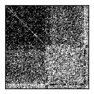
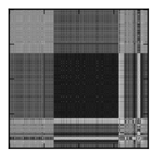
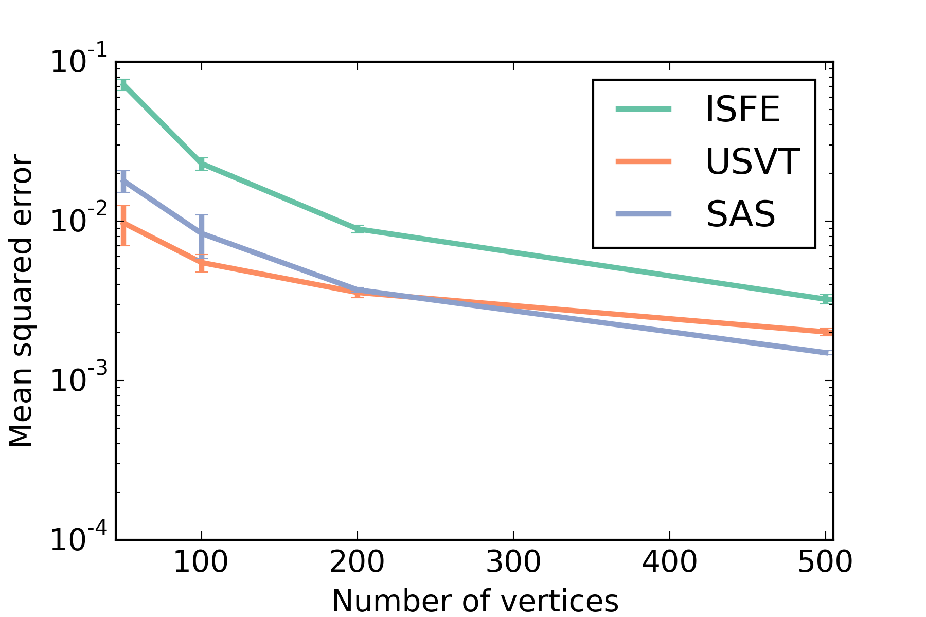
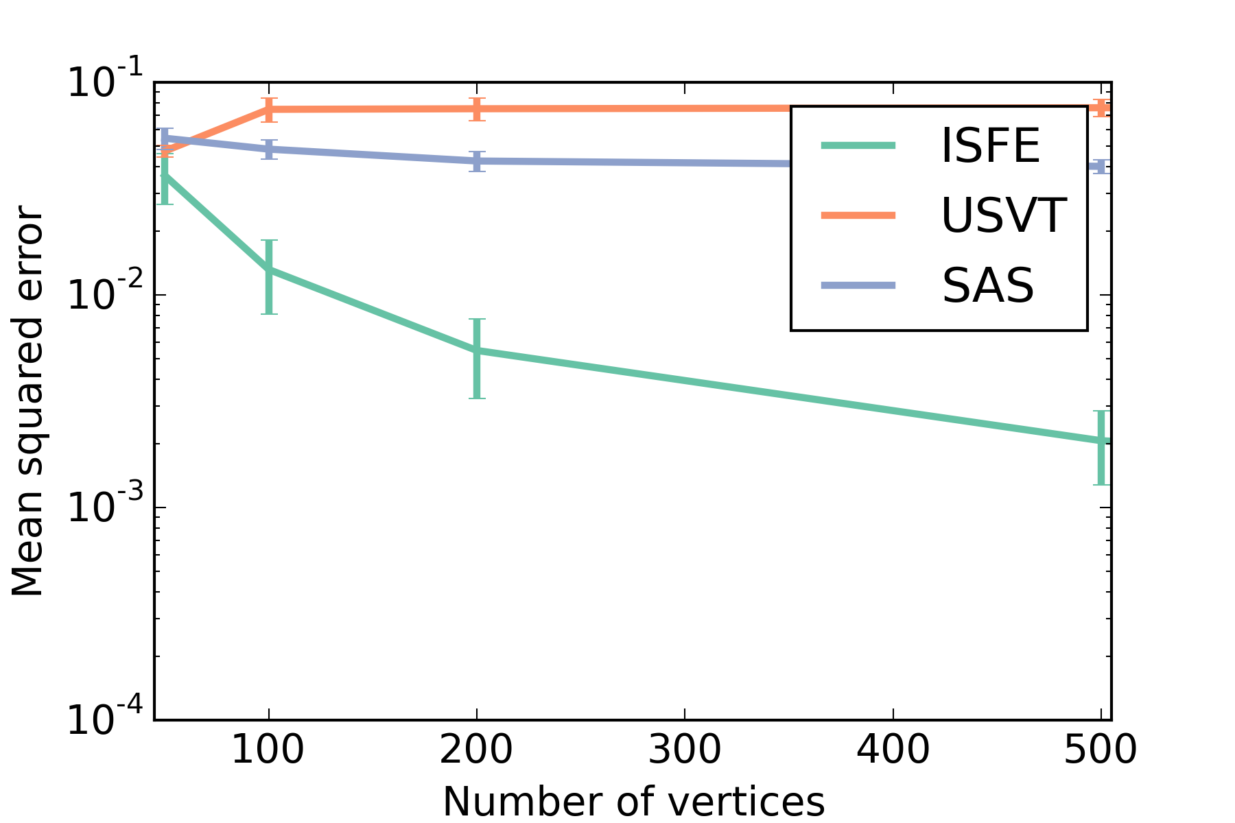
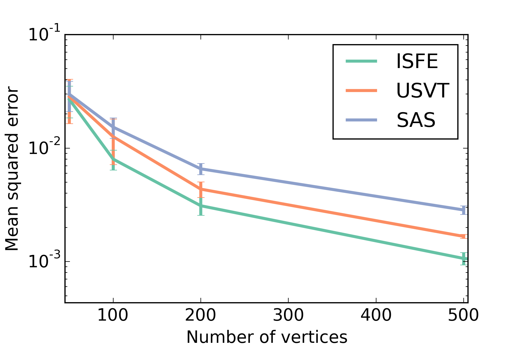
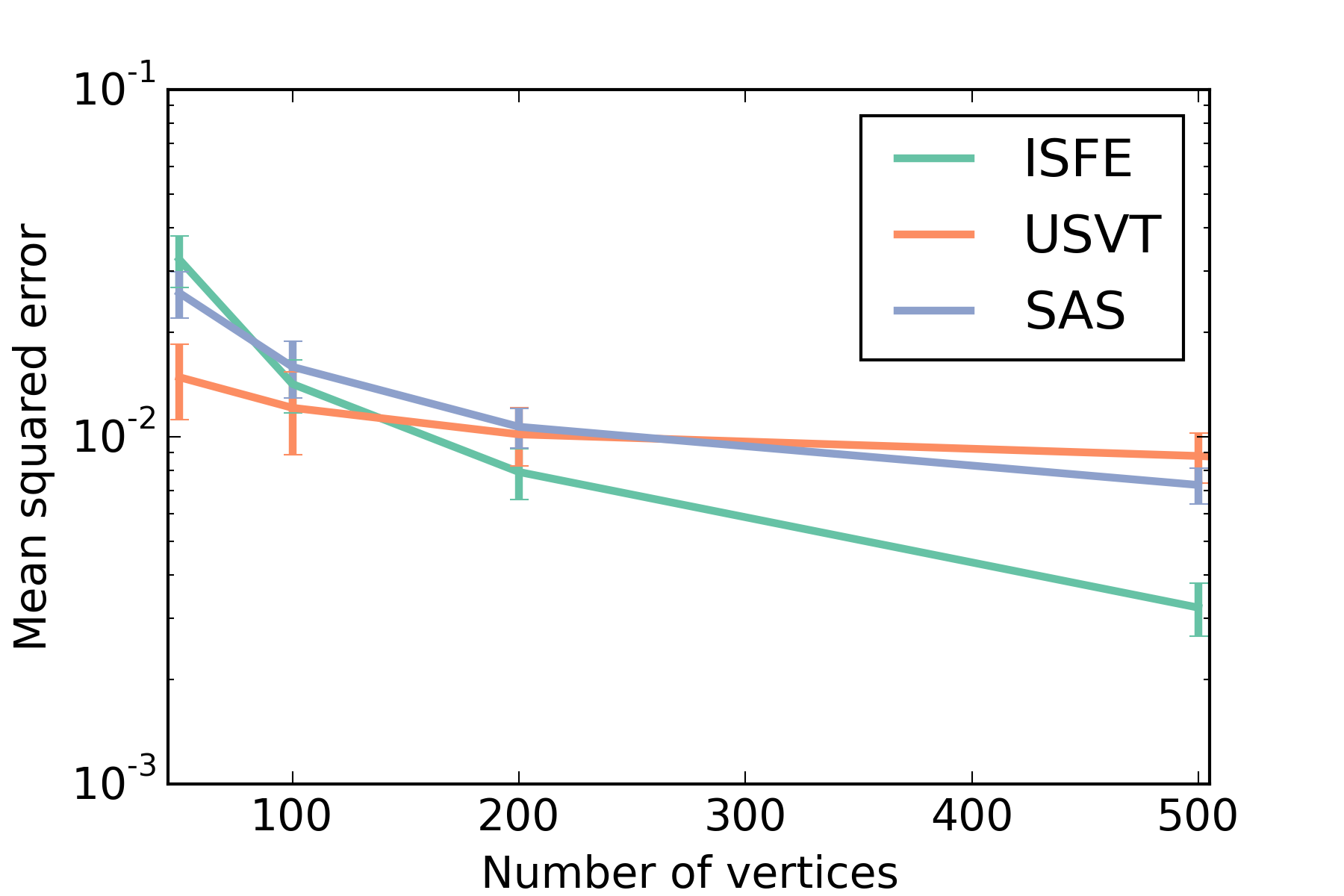
We examine synthetic data sampled from several graphons: (1) a gradient graphon given by the function $W(x,y)=\frac{(1-x)+(1-y)}{2}$; (2) an SBM graphon with $p=0.5$, $q=(0.7,0.3)$; (3) an SBM graphon with $p=0.3$, $q=(0.7,0.3)$; and (4) an IRM graphon with $\alpha=3,a=3,b=2.9$. In Figure 4, we display the results of ISFE and two other estimators on a 200 vertex sample from each of the graphons. The first column displays the graphon, the second column is the result of ISFE on the sample (starting with the trivial partition), the third column shows the result of SAS (Chan and Airoldi, 2014), and the last column shows the result of USVT (Chatterjee, 2014). We display in Figure 5 the MSE of each estimation method on samples from the graphons listed above for varying sizes of $n$, averaged over 50 independent draws.

We evaluate all estimators using the mean squared error (MSE) given in Equation (3) for the graphon value estimator $\widehat{M}$ we describe below. For ISFE, we consider the graphon value estimator $\widehat{M}$ described in Section 3.3; the parameter $\ell$ was set to the value that minimized the MSE over a grid of values; the gradient graphon used $\ell=20$, the SBM graphon with $p=0.5$ used $\ell=8$, the SBM graphon with $p=0.3$ used $\ell=10$, and the IRM graphon used $\ell=15$. For a 200-vertex sample from the IRM graphon, ISFE took 3.4 seconds to complete for $T=3$ (using 8 GB RAM and 4 cores at 2.8 GHz). For a fixed partition size, there is a limit to how well one can approximate the graphon in MSE. Hence after some number of iterations, ISFE will cease to improve. We therefore set the number of iterations $T$ to be the first value after which the MSE no longer improved by at least $10^{-3}$.

We modified SAS by minimizing the total variation distance using a general-purpose constrained optimization method instead of using the alternating direction method of multipliers. For USVT, we follow Chan and Airoldi (2014) and first sort the sample by degree. SAS and USVT expect graphons with monotonizable degree distribution. In order to exhibit these estimation techniques for arbitrary graphons, we take $\widehat{M}$ to be a permutation of their estimated matrix, rearrranged so as to invert the way vertices from the sampled graph were sorted.

For all graphon estimator images, we re-sort the result by increasing $U_{i}$ so that the result can be visually compared to the original graphon. While MSE is directly a measure of similarity between this re-sorted estimate and the original graphon (evaluated at certain points), in some cases better upper-bounds on the MISE may be obtained from other rearrangements of the estimate. Indeed, the smoothed function estimates obtained by SAS and USVT for the gradient lead to a considerably smaller upper-bound on the MISE than their displayed re-sorted estimates (and than the original value estimates by USVT).

(a) Gradient.

(b) SBM, $p=0.5,q=(0.7,0.3)$.

(c) SBM, $p=0.3,q=(0.7,0.3)$.

(d) IRM, $\alpha=3,a=3,b=2.9$.

Figure 4: Comparison of graphon estimation methods ISFE, SAS, and USVT. Rows: (a) Gradient graphon, (b) SBM graphon, $p=0.5,q=(0.7,0.3)$, (c) SBM graphon, $p=0.3,q=(0.7,0.3)$, and (d) IRM graphon, $\alpha=3,a=3,b=2.9$. Columns: (1) The original graphon, (2) ISFE (beginning with the trivial partition), (3) SAS, and (4) USVT. All estimator images are sorted by increasing $U_{i}$.

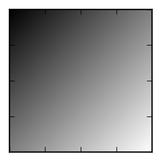
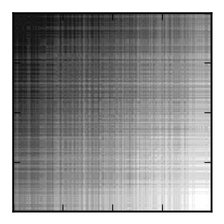
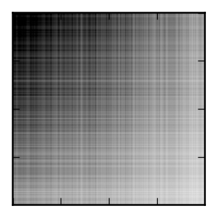
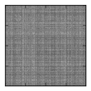
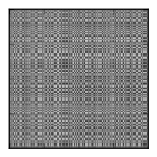
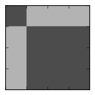
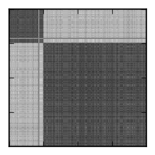
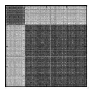
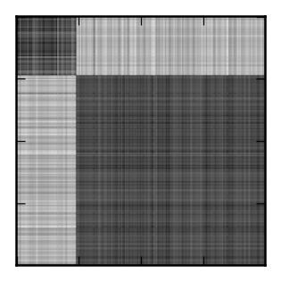
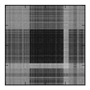
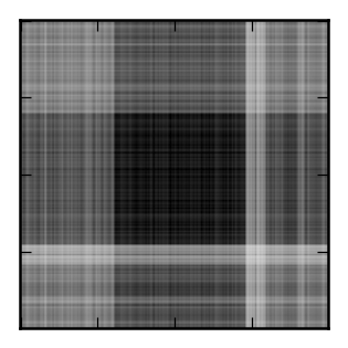
SAS and USVT perform well not only for graphons with monotonizable degree distribution, such as gradients (as in Figure 4(a)), for which SAS was explicitly designed, but also ones that are monotonizable up to some partition (as in Figures 4(c) and 4(d)). However, when the degree distribution is constant over regions with different structure (as in Figure 4(b)), SAS and USVT fail to discern this structure. In contrast, ISFE is able to recover much of the structure after a small number of iterations, even when it begins with no structural information, i.e., the trivial partition.

(a) Gradient

(b) SBM, $p=0.5$

(c) SBM, $p=0.3$

(d) IRM

Figure 5: MSE of ISFE, USVT, and SAS estimators on independent samples from gradient graphon, SBM graphon, $p=0.5,q=(0.7,0.3)$, SBM graphon, $p=0.3,q=(0.7,0.3)$, IRM graphon, $\alpha=3,a=3,b=2.9$. Error bars represent the standard deviation.

In Appendix C, we examine the result of ISFE on three real-world social network datasets. The question of how to model sparse graphs remains an important open problem, as we discuss in Appendix C. To demonstrate our graphon estimator, we sidestep these issues to some extent by considering a denser subgraph of the original network.

6 Discussion

While any clustering algorithm naturally induces a graphon estimator, we have described and shown some of the improvements that may be obtained by grouping vertices according to their average edge densities with respect to the clusters. The fact that such improvements are possible is unsurprising for graphs admitting block structure (although there are many possible refinements and further analysis of the algorithm we describe). Indeed, arbitrary graphons are well-approximated by step-function graphons in the cut metric, and step-functions graphons (which arise as models in the stochastic block model and elsewhere) are well-approximated by such in $L^{2}$. A key problem is to devise graphon estimators that further leverage this structure.

Acknowledgments

The authors would like to thank Daniel Roy for detailed comments on a draft, and James Lloyd and Peter Orbanz for helpful conversations.

This material is based upon work supported by the United States Air Force and the Defense Advanced Research Projects Agency (DARPA) under Contract Numbers FA8750-14-C-0001 and FA8750-14-2-0004. Work by C. F. was also made possible through the support of Army Research Office grant number W911NF-13-1-0212 and a grant from Google. Any opinions, findings and conclusions or recommendations expressed in this material are those of the authors and do not necessarily reflect the views of the United States Air Force, Army, or DARPA.

Appendix A Measures of risk for graphons

A.1 The cut metric

The cut metric defines a notion of distance between two graphs or graphons. We begin by defining it for finite graphs on the same vertex set, following §8.1 and §8.2 of Lovász (2012).

Definition A.1.

Let $F,G$ be two graphs on $[n]$. The cut metric between $F$ and $G$ is given by

$$d_{\Box}(F,G):=\max_{S,T\subseteq[n]}\frac{|c_{F}(S,T)-c_{G}(S,T)|}{n^{2}}.$$ (4)

Note that the denominator of Equation (4) is $n^{2}$ regardless of the size of $S$ and $T$; having large distance between $F$ and $G$ in the cut metric implies that there is some large vertex set on which their respective edge densities differ.

The cut distance $\delta_{\Box}$ between two graphs on different vertex sets of the same size $n$ is then defined to be the minimum of $d_{\Box}$ over all relabelings of $F$ and $G$ by $[n]$. While the cut distance can be extended to arbitrary finite weighted graphs on different vertex sets, these definitions are rather technical, and so we instead define the analogous quantity for graphons, from which one may inherit the corresponding notions via step-function graphons.

Definition A.2.

Let $W,V$ be graphons. The cut metric between $W$ and $V$ is given by

$$d_{\Box}(W,V):=\sup_{S,T\subseteq[0,1]}\left|\int_{S\times T}\bigl{(}W(x,y)-V(x,y)\bigr{)}\,dx\,dy\right|,$$

where $S$ and $T$ range over measurable subsets. The cut distance between $W$ and $V$ is defined to be

$$\delta_{\Box}(W,V):=\inf_{\varphi}\,d_{\Box}(W,V^{\varphi}),$$

where $\varphi$ is a measure-preserving transformation of $[0,1]$.

Note that the cut distance is only a pseudometric, as it is zero for weakly isomorphic graphons.

By the Frieze–Kannan weak regularity lemma (Frieze and Kannan, 1999a, b), step-functions approximate graphons in the cut distance, where the required number of steps depends only on the desired accuracy, not the choice of graphon.

Lemma A.3 (Weak regularity (Lovász, 2012, Lemma 9.3)).

For every $k\geq 1$ and any graph $G$, there is a partition $\mathcal{P}$ of the vertices of $G$ into $k$ classes such that

$$\delta_{\Box}(G,W_{G/\mathcal{P}})\leq\frac{2}{\sqrt{\log k}}.$$

An analogous statement holds for graphons (Lovász, 2012, Corollary 9.13). Step-functions also approximate graphons arbitrarily well in $L^{1}$ distance (or $L^{2}$, as in MSE or MISE), but the convergence is not uniform in the choice of graphon (Lovász, 2012, Proposition 9.8).

A.2 $L^{2}$ and the cut distance

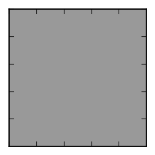
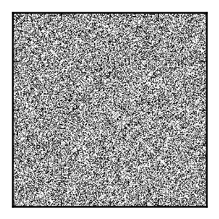
In graphon estimation by step-functions, we are given a finite graph sampled from a graphon, and need to choose the number of steps by which to approximate the graphon. Under $L^{2}$ risk, the number of such steps could be arbitrarily large depending on the particular graphon. But moreover, this number can vary wildly even among graphons that give rise to similar distributions — which therefore must be close in the cut distance (Lovász, 2012, Lemma 10.31). For example (Janson, 2013, Example 10.11), this can be seen by considering a constant function graphon $W$ (whose samples are Erdős–Rényi graphs) and the step-function graphon $V_{k}$ induced by a graph of size $k$ sampled from $W$. (For an illustration of $W$ and $V_{k}$, see Figure 6.) Their samples $\mathbb{G}(n,W)$ and $\mathbb{G}(n,V_{k})$ have similar distributions, and indeed $\delta_{\Box}(W,V_{k})=O(1/\sqrt{k})$, even though the $L^{1}$ distance between $W$ and $V_{k}$ is roughly $1/2$ regardless of $k$ (and hence $L^{2}$ also does not decrease in $k$). For this reason, it may be more appropriate to consider risk based on the cut distance, rather than the $L^{2}$-based MISE, for the function estimation problem for arbitrary graphons.

On the other hand, both the cut metric and $L^{1}$ can be close for step-functions (Lovász, 2012, Equation (8.15)). Hence even in $L^{1}$ (or $L^{2}$), it can be more reasonable to approximate a step-function graphon (as opposed to an arbitrary graphon) by step-function graphons.

Furthermore, while a large $L^{2}$ distance between graphons does not guarantee that they are far in the cut distance, a small $L^{2}$ distance does provide an upper bound on cut distance (and hence on the total variation distance between the distributions on small subsamples). Indeed, in many cases (as in our empirical results here), one is in fact able to produce good bounds on $L^{2}$.

Figure 6: Example of graphons that are close in the cut distance but are far in $L^{1}$ (and $L^{2}$). (left) The constant graphon $W=1/2$. (right) The graphon $V_{1000}$ obtained as the step-function of a sample from $\mathbb{G}(1000,W)$.

Appendix B Further discussion and analysis of ISFE

B.1 ISFE for step-functions of finite graphs

If one clusters the vertices of a sampled graph discretely, by assigning one class for each vertex, this typically induces a poor graphon estimator, as the reported graphon is merely the step-function of the sample. On the other hand, if we perform even a single iteration of ISFE on such a partition, we obtain an estimator that clusters vertices according to the Hamming distances between their edge vectors. In the case where the original graphon is the step-function of some finite graph on $n$ vertices, ISFE following such a partition can recover the original graphon exactly in the sense of MSE, so long as the requested partition size is at least $n$. (Estimation with respect to MISE is limited only by the extent to which the sampled graph distorts the proportion of vertices arising from each vertex of the original.)

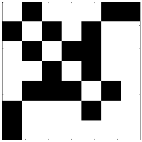
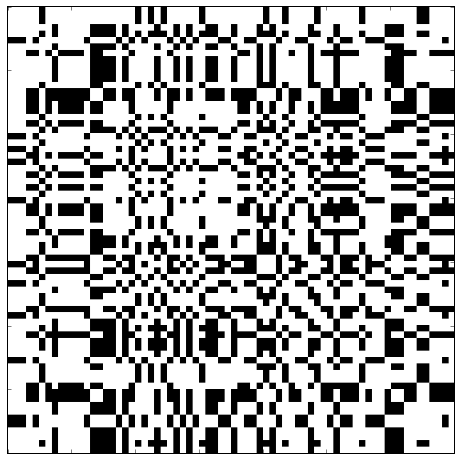
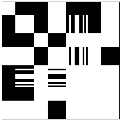
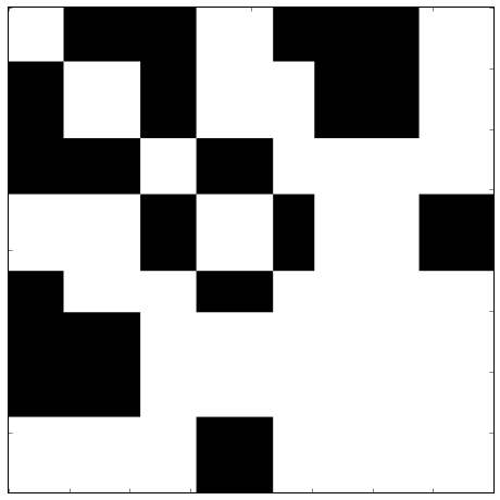
We present an example in Figure 7. In this example, we form the step-function graphon $W_{G}$ of a graph $G$ with $7$ vertices; its adjacency matrix can be seen via the black and white squares in Figure 7(a). ISFE is run on a $70$ vertex sample (Figure 7(b)) for a single iteration starting from the partition with every vertex in its own class. This single iteration amounts to forming a partition based on Hamming distance on the vector of edges for each vertex (i.e., rows of the adjacency matrix); so long as the requested number of bins is at least 7, the original structure will be recovered. The resulting graphon from ISFE in Figure 7(d) and the original step-function graphon in Figure 7(a) are not weakly isomorphic, because some of the 7 steps of the original resulted in slightly more or fewer than 10 vertices in the sample, but they are very close in the cut distance and, after rearranging by a measure-preserving transformation, in $L^{1}$. Note that sorting by degree (Figure 7(c)) garbles the structure among those regions corresponding to distinct vertices of the original having the same degree.

(a) Step-function

(b) Sampled graph

(c) Sorted by degree

(d) Hamming

Figure 7: (a) Black and white step-function graphon of a $7$ vertex graph; (b) a 70 vertex sample from the step-function; (c) result of sorting the sample by degree; (d) result of binning the sample using Hamming distance.

B.2 ISFE for stochastic block models

We now discuss the behavior of a variant of ISFE on a $2$-step stochastic block model. We show that given a partition of the vertices, in which a large portion of the vertices in each class are correctly classified (i.e., the vertices are in the same class as their true class according to the SBM), with high probability the ISFE algorithm will improve (by an arbitrary amount) the fraction of vertices that are classified correctly.

In this variant of ISFE, centroids are chosen randomly (as described below) rather than greedily; while this makes the algorithm easier to analyze, one expects that ISFE as described and evaluated empirically elsewhere in the paper should perform at least as well in most circumstances.

Let $W$ be a step-function graphon describing a stochastic block model, with $2$ steps $A,B$ of respective sizes $p$ and $1-p$, where $p\leq\frac{1}{2}$. Let $q_{0}$ be the edge density within each class and $q_{1}$ the edge density across the two classes, and assume $q_{0}>q_{1}$.

Let $G$ be a graph on $[n]$ sampled from $\mathbb{G}(n,W)$. Let ${G^{\dagger}}$ be the (not necessarily simple) graph obtained from $G$ by adding a self-loop at vertex $i$ with probability $q_{0}$ independently for each $i\in[n]$. Note that ${G^{\dagger}}$ can be thought of as the result of a modified sampling procedure from $W$, where we instead assign self-loops with the same probability as other edges within a class. We will find that many of our calculations are more easily done in terms of ${G^{\dagger}}$.

Considering how each vertex of $G$ was sampled according to $\mathbb{G}(n,W)$, define the following sets:

$$[n]_{A} := \{x\in[n]\,{\,:\,}\,x\text{~{}came from~{}}A\}\text{~{}and}$$

$$\ [n]_{B} := \{x\in[n]\,{\,:\,}\,x\text{~{}came from~{}}B\}.$$

Suppose the algorithm begins with a partition $\{C_{1},\ldots,C_{k}\}$ of the vertices $[n]$ into $k\geq 2$ classes. For each $i\in[k]$, define

$$C^{*}_{i}:=\begin{cases}[n]_{A}\cap C_{i}&\text{if~{}}\bigl{|}[n]_{A}\cap C_{i}\bigr{|}\,\geq\,\bigl{|}[n]_{B}\cap C_{i}\bigr{|},\text{~{}and}\\ [n]_{B}\cap C_{i}&\text{otherwise}.\end{cases}$$

For $i\in[k]$ we call $C^{*}_{i}$ the majority of $C_{i}$, and for each vertex $x\in C_{i}$ we say that $x$ is correctly classified when $x\in C^{*}_{i}$. Define

$$K_{A} := \{i\in[k]:C^{*}_{i}\subseteq[n]_{A}\},\text{~{}and}$$

$$K_{B} := \{i\in[k]:C^{*}_{i}\subseteq[n]_{B}\}.$$

Recall that given a vertex $x\in[n]$, we define its weighted edge-density vector to be

$$\textstyle e_{x}:=\bigl{[}\frac{|C_{1}|}{n}\,e_{G}(x,C_{1}),\ldots,\frac{|C_{k}|}{n}\,e_{G}(x,C_{k})\bigr{]}.$$

Let $\tau$ be such that at least a $\tau$-fraction of vertices in $[n]$ are correctly classified by the partition $\{C_{1},\ldots,C_{k}\}$, i.e.,

$$\sum_{i\in[k]}|C^{*}_{i}|\geq\tau n.$$

Given arbitrary $\tau^{\prime}>\tau$, our goal is to give a lower bound on the probability that, after applying the variant of ISFE we describe here, the resulting partition correctly classifies at least a fraction $\tau^{\prime}$ of vertices.

We now analyze one iteration of this variant of ISFE beginning with a partition $\{C_{1},\ldots,C_{k}\}$. We create a new partition by first selecting $k$ many centroids uniformly independently at random from $[n]$ without replacement, and then we assign every remaining (i.e., non-centroid) vertex $x\in[n]$ to the bin whose centroid’s weighted edge-density vector is closest in $L^{1}$ to the weighted edge-density vector $e_{x}$ (breaking ties uniformly independently at random).

Definition B.1.

For $\delta>0$, define a class $C_{i}$ to be $\delta$-large when $|C_{i}|\geq\delta\frac{n}{k}$. We say that a $\delta$-large class $C_{i}$ is $\delta$-good when $\frac{|C^{*}_{i}|}{|C_{i}|}\geq\delta$ further holds, i.e., a large fraction of its vertices are correctly classified. Define

$$D_{\delta}:=\{i\in[k]\,{\,:\,}\,C_{i}\text{~{}is~{}$\delta$-large~{}and~{}$\delta$-good}\}.$$

Note that for $i\in D_{\delta}$, with high probability, the edge density of each vertex $x\in[n]$ with respect to $C_{i}$ will be close to its true edge density, i.e., $q_{0}$ if either

$$x\in[n]_{A}\text{~{}and~{}}C^{*}_{i}\subseteq[n]_{A}$$

or

$$x\in[n]_{B}\text{~{}and~{}}C^{*}_{i}\subseteq[n]_{B},$$

and $q_{1}$ otherwise.

Lemma B.2.

Suppose $C_{i}$ is $\delta$-large. If $\delta-\delta^{2}\geq k\,(1-\tau)$, then $C_{i}$ is $\delta$-good.

Proof.

By our assumption on $\tau$ we know that

$$|C_{i}\setminus C^{*}_{i}|\leq n\,(1-\tau).$$

Hence

$$\frac{|C^{*}_{i}|}{|C_{i}|} =1-\frac{|C_{i}\setminus C^{*}_{i}|}{|C_{i}|}\geq 1-\frac{n\,(1-\tau)}{|C_{i}|}$$

$$\geq 1-\frac{n\,(1-\tau)}{\delta\,\frac{n}{k}}=1-\frac{k\,(1-\tau)}{\delta}.$$

But $1-\frac{k\,(1-\tau)}{\delta}\geq\delta$ because $\delta-\delta^{2}\geq k\,(1-\tau)$. Hence $C_{i}$ is $\delta$-good. ∎

In other words, if $k$ is not too large with respect to $\tau$, and $\delta$ is sufficiently large, then every $\delta$-large class must also be $\delta$-good. Hence if most vertices $x$ are such that for $\epsilon$ close to $0$ and $\delta$ close to $1$, for every $\delta$-good class, the density of $x$ with respect to the majority of that class is within $\epsilon$ of its expected value, then the step-function graphon determined by the partition $\{C_{1},\ldots,C_{k}\}$ gives rise to a graphon value estimate of $W$ that yields a small MSE. We make this notion precise by defining $(\epsilon,\delta)$-good vertices.

Throughout the rest of this section, we omit brackets for singleton classes, and write, e.g., $e_{G}(x,C_{i})$ in place of $e_{G}(\{x\},C_{i})$.

Definition B.3.

For $\epsilon,\delta>0$ we say that a vertex $x\in[n]_{A}$ is $(\epsilon,\delta)$-good when for all $i\in D_{\delta}$, if $i\in K_{A}$ then

$$|e_{{G^{\dagger}}}(x,C^{*}_{i})-q_{0}|<\epsilon$$

and if $i\in K_{B}$ then

$$|e_{{G^{\dagger}}}(x,C^{*}_{i})-q_{1}|<\epsilon.$$

Similarly, we say that a vertex $x\in[n]_{B}$ is $(\epsilon,\delta)$-good when for all $i\in D_{\delta}$, if $i\in K_{B}$ then

$$|e_{{G^{\dagger}}}(x,C^{*}_{i})-q_{0}|<\epsilon$$

and if $i\in K_{A}$ then

$$|e_{{G^{\dagger}}}(x,C^{*}_{i})-q_{1}|<\epsilon.$$

We let $\mathfrak{G}_{\epsilon,\delta}(x)$ be the event that $x$ is $(\epsilon,\delta)$-good.

In other words, $x$ is $(\epsilon,\delta)$-good if for every $\delta$-good class, the density of $x$ with respect to the majority of that class is within $\epsilon$ of its expected value.

We will begin by showing that if each of the centroids is $(\epsilon,\delta)$-good (for an appropriate $\epsilon$ and $\delta$), then each $(\epsilon,\delta)$-good vertex is correctly classified. This will then reduce the task of giving bounds on the probability that at least $\tau^{\prime}n$ vertices are correctly classified to that of giving bounds on the probability that at least $\tau^{\prime}n$ vertices are $(\epsilon,\delta)$-good.

Proposition B.4.

Suppose that each centroid is $(\epsilon,\delta)$-good, and that at least one centroid is in $[n]_{A}$ and at least one centroid is in $[n]_{B}$. Further suppose that

$$\textstyle q_{0}-q_{1}\geq 2(\frac{2-\delta}{\tau}-1+2\epsilon+\frac{k}{n\delta\tau}).$$

Then the weighted edge-density vector of each $(\epsilon,\delta)$-good vertex of $[n]_{A}$ is closer in $L^{1}$ to that of some centroid in $[n]_{A}$ than to that of any centroid in $[n]_{B}$. Similarly, the weighted edge-density vector of each $(\epsilon,\delta)$-good vertex of $[n]_{B}$ is closest to that of a centroid in $[n]_{B}$.

Proof.

For each $(\epsilon,\delta)$-good vertex $d_{A}\in[n]_{A}$, and each $(\epsilon,\delta)$-good vertex $d_{B}\in[n]_{B}$, each $i_{A}\in K_{A}\cap D_{\delta}$, and $i_{B}\in K_{B}\cap D_{\delta}$ we have

$$\tau(q_{0}-\epsilon) \leq e_{G^{\dagger}}(d_{A},C_{i_{A}})\leq\tau(q_{0}+\epsilon)+1-\tau,$$

$$\tau(q_{1}-\epsilon) \leq e_{G^{\dagger}}(d_{A},C_{i_{B}})\leq\tau(q_{1}+\epsilon)+1-\tau,$$

$$\tau(q_{1}-\epsilon) \leq e_{G^{\dagger}}(d_{B},C_{i_{A}})\leq\tau(q_{1}+\epsilon)+1-\tau,\text{~{}and}$$

$$\tau(q_{0}-\epsilon) \leq e_{G^{\dagger}}(d_{B},C_{i_{B}})\leq\tau(q_{0}+\epsilon)+1-\tau.$$

Hence we also have

$$\textstyle\tau(q_{0}-\epsilon)-\frac{1}{|C_{i_{A}}|} \leq e_{G}(d_{A},C_{i_{A}})\leq\tau(q_{0}+\epsilon)+1-\tau,$$

$$\textstyle\tau(q_{1}-\epsilon)-\frac{1}{|C_{i_{B}}|} \leq e_{G}(d_{A},C_{i_{B}})\leq\tau(q_{1}+\epsilon)+1-\tau,$$

$$\textstyle\tau(q_{1}-\epsilon)-\frac{1}{|C_{i_{A}}|} \leq e_{G}(d_{B},C_{i_{A}})\leq\tau(q_{1}+\epsilon)+1-\tau,\text{~{}and}$$

$$\textstyle\tau(q_{0}-\epsilon)-\frac{1}{|C_{i_{B}}|} \leq e_{G}(d_{B},C_{i_{B}})\leq\tau(q_{0}+\epsilon)+1-\tau,$$

where the differences come from the fact that in ${G^{\dagger}}$ we may add self-loops, and that $d_{A}$ and $d_{B}$ are themselves in some class. Further, as $|C_{i}|\geq\frac{n}{k}\delta$, we have

$$\textstyle\tau(q_{0}-\epsilon)-\frac{k}{n\delta} \leq e_{G}(d_{A},C_{i_{A}})\leq\tau(q_{0}+\epsilon)+1-\tau,$$

$$\textstyle\tau(q_{1}-\epsilon)-\frac{k}{n\delta} \leq e_{G}(d_{A},C_{i_{B}})\leq\tau(q_{1}+\epsilon)+1-\tau,$$

$$\textstyle\tau(q_{1}-\epsilon)-\frac{k}{n\delta} \leq e_{G}(d_{B},C_{i_{A}})\leq\tau(q_{1}+\epsilon)+1-\tau,\text{~{}and}$$

$$\textstyle\tau(q_{0}-\epsilon)-\frac{k}{n\delta} \leq e_{G}(d_{B},C_{i_{B}})\leq\tau(q_{0}+\epsilon)+1-\tau.$$

We first consider the $L^{1}$ distance between the weighted edge-density vectors of a vertex from $[n]_{A}$ and a vertex $x$. Again assume the vertex $d_{A}\in[n]_{A}$ is $(\epsilon,\delta)$-good, and suppose $x\in[n]_{A}$ is an $(\epsilon,\delta)$-good vertex. For $i_{A}\in K_{A}$ we have

$$|e_{G}(x,C_{i_{A}})-e_{G}(d_{A},C_{i_{A}})| \leq (\tau(q_{0}+\epsilon)+1-\tau)-\tau(q_{0}-\epsilon)+\tfrac{k}{n\delta}$$

$$= 2\tau\epsilon+1-\tau+\tfrac{k}{n\delta},$$

and for $i_{B}\in K_{B}$ we have

$$|e_{G}(x,C_{i_{B}})-e_{G}(d_{A},C_{i_{B}})| \leq (\tau(q_{1}+\epsilon)+1-\tau)-\tau(q_{1}-\epsilon)+\tfrac{k}{n\delta}$$

$$= 2\tau\epsilon+1-\tau+\tfrac{k}{n\delta}.$$

Further,

$$\textstyle(k-1)\,(1-\delta)\,\frac{n}{k}<(1-\delta)\,n,$$

and so at most $(1-\delta)\,n$ many vertices are not in classes with respect to which they are $\delta$-good. Hence the $L^{1}$ distance between the weighted edge-density vectors

$$\textstyle e_{x}=\bigl{[}\frac{|C_{1}|}{n}\,e_{G}(x,C_{1}),\ldots,\frac{|C_{k}|}{n}\,e_{G}(x,C_{k})\bigr{]}$$

and

$$\textstyle e_{d_{A}}=\bigl{[}\frac{|C_{1}|}{n}\,e_{G}(d_{A},C_{1}),\ldots,\frac{|C_{k}|}{n}\,e_{G}(d_{A},C_{k})\bigr{]}$$

is equal to

$$\frac{1}{n}\sum_{i\in[k]}|C_{i}|\,\bigl{|}e_{G}(x,C_{i})-e_{G}(d_{A},C_{i})\bigr{|},$$

which is at most

$$\textstyle\frac{1}{n}\bigl{(}(1-\delta)\,n+\sum_{i\in[k]}|C_{i}|\,(2\tau\epsilon+1-\tau+\frac{k}{n\delta})\bigr{)}.$$

Hence the $L^{1}$ distance is at most

$$(1-\delta)+2\tau\epsilon+1-\tau+\frac{k}{n\delta},$$

as $\sum_{i\in[k]}|C_{i}|=n$.

Now let $d_{B}\in[n]_{B}$ be $(\epsilon,\delta)$-good. We now consider the $L^{1}$ distance between the weighted edge-density vectors $e_{d_{B}}$ and $e_{x}$. As $q_{0}>q_{1}$, for $i_{A}\in K_{A}$ we have

$$|e_{G}(x,C_{i_{A}})-e_{G}(d_{B},C_{i_{A}})| \geq \tau(q_{0}-\epsilon)-\tfrac{k}{n\delta}-(\tau(q_{1}+\epsilon)+1-\tau))$$

$$= \tau(q_{0}-q_{1}-2\epsilon)-\tfrac{k}{n\delta}-1+\tau,$$

and for $i_{B}\in K_{B}$ we have

$$|e_{G}(x,C_{i_{B}})-e_{G}(d_{B},C_{i_{B}})| \geq \tau(q_{0}-\epsilon)-\tfrac{k}{n\delta}-(\tau(q_{1}+\epsilon)+1-\tau))$$

$$= \tau(q_{0}-q_{1}-2\epsilon)-\tfrac{k}{n\delta}-1+\tau.$$

Therefore the $L^{1}$-distance between the weighted edge-density vectors $e_{x}$ and

$$\textstyle e_{d_{B}}=\bigl{[}\frac{|C_{1}|}{n}\,e_{G}(d_{B},C_{1}),\ldots,\frac{|C_{k}|}{n}\,e_{G}(d_{B},C_{k})\bigr{]}$$

is at least

$$\textstyle\frac{1}{n}\bigl{(}-(1-\delta)n+\sum_{i\in[k]}|C_{i}|\,(\tau(q_{0}-q_{1}-2\epsilon)-\frac{k}{n\delta}-1+\tau)\bigr{)}\ =\ -(1-\delta)+\tau(q_{0}-q_{1}-2\epsilon)-\frac{k}{n\delta}-1+\tau.$$

In particular, if

$$\textstyle-(1-\delta)+\tau(q_{0}-q_{1}-2\epsilon)-\frac{k}{n\delta}-1+\tau\geq(1-\delta)+2\tau\epsilon+1-\tau+\frac{k}{n\delta},$$

then $e_{x}$ is closer in $L^{1}$ to $e_{d_{A}}$ than to $e_{d_{B}}$ whenever $d_{A}\in[n]_{A}$ and $d_{B}\in[n]_{B}$ are $(\epsilon,\delta)$-good. But this inequality is equivalent to our hypothesis,

$$\textstyle q_{0}-q_{1}\geq 2(\frac{2-\delta}{\tau}-1+2\epsilon+\frac{k}{n\delta\tau}).$$

Hence, as we have assumed that all centroids are $(\epsilon,\delta)$-good, the vertex $x$ is placed in a class whose centroid is in $[n]_{A}$. A similar argument shows that if $x\in[n]_{B}$ is $(\epsilon,\delta)$-good then $x$ is placed in a class whose centroid is in $[n]_{B}$. ∎

Recall that $\mathfrak{G}_{\epsilon,\delta}(x)$ is the event that a vertex $x$ is $(\epsilon,\delta)$-good. Notice that for each $x_{A},y_{A}\in[n]_{A}$,

$$\Pr(\mathfrak{G}_{\epsilon,\delta}(x_{A}))=\Pr(\mathfrak{G}_{\epsilon,\delta}(y_{A})),$$

and for each $x_{B},y_{B}\in[n]_{B}$,

$$\Pr(\mathfrak{G}_{\epsilon,\delta}(x_{B}))=\Pr(\mathfrak{G}_{\epsilon,\delta}(y_{B})).$$

We now want to give a lower bound for these values. For $n\in{{\mathbb{N}}}$ and $\zeta\in[0,1]$, let $X_{n,\zeta}\sim\frac{1}{n}\operatorname{Binomial}(n,\zeta)$, and for $\epsilon>0$ define

$$\mathcal{B}(n,\zeta,\epsilon):=\Pr\bigl{(}\bigl{|}X_{n,\zeta}-\zeta\bigr{|}\,<\,\epsilon\bigr{)}.$$

Note that we also have

$$\mathcal{B}(n,\zeta,\epsilon)=\Pr\bigl{(}\bigl{|}n\,X_{n,\zeta}-n\,\zeta\bigr{|}\,<\,n\,\epsilon\bigr{)},$$

i.e., the probability that the number of successful trials differs from the expected number by at most $n\,\epsilon$.

It is then easily checked, using Chernoff’s bound, that the following inequality holds:

$$\mathcal{B}(n,\zeta,\epsilon)\geq 1-2\,\exp\left\{-\frac{\epsilon^{2}\,n}{3\zeta}\right\}.$$

We now use this inequality to bound the probability that a given vertex is $(\epsilon,\delta)$-good.

Lemma B.5.

For all $x\in[n]$,

$$\Pr\bigl{(}\mathfrak{G}_{\epsilon,\delta}(x)\bigr{)}\geq\left(1-2\,\exp\left\{-\frac{\epsilon^{2}\,\delta^{2}n}{3k}\right\}\right)^{k}.$$

Proof.

Note that when $i\in K_{A}$ is such that $C_{i}$ is $\delta$-good, we have $\frac{|C^{*}_{i}|}{|C_{i}|}\geq\delta$ and $|C_{i}|\geq\delta\frac{n}{k}$, and so $|C^{*}_{i}|\geq\delta^{2}\frac{n}{k}$.

Let ${\mathfrak{F}_{J,H}(x,i)}$ denote the event that $x\in[n]_{J}$ and $i\in K_{H}$, where $J,H\in\{A,B\}$. Observe that conditioning on ${\mathfrak{F}_{A,A}(x,i)}$, we have that $e_{G^{\dagger}}(x,C^{*}_{i})$ has the same distribution as $X_{|C^{*}_{i}|,q_{0}}$, and so $\mathbb{E}\bigl{(}e_{G^{\dagger}}(x,C^{*}_{i})\,\big{|}\,{\mathfrak{F}_{A,A}(x,i)}\bigr{)}=q_{0}$ and

$$\mathbb{E}\bigl{(}c_{G^{\dagger}}(x,C^{*}_{i})\,\big{|}\,{\mathfrak{F}_{A,A}(x,i)}\bigr{)}=\mathbb{E}\bigl{(}|C^{*}_{i}|\,e_{G^{\dagger}}(x,C^{*}_{i})\,\big{|}\,{\mathfrak{F}_{A,A}(x,i)}\bigl{)}=q_{0}\,|C^{*}_{i}|.$$

We therefore also have

$$\Pr\bigl{(}|e_{G^{\dagger}}(x,C^{*}_{i})-q_{0}|<\epsilon\ \big{|}\ {\mathfrak{F}_{A,A}(x,i)}\bigr{)} = \mathcal{B}(|C^{*}_{i}|,q_{0},\epsilon)$$

$$\geq 1-2\,\exp\left\{-\frac{\epsilon^{2}\,|C^{*}_{i}|}{3q_{0}}\right\}$$

$$\geq 1-2\,\exp\left\{-\frac{\epsilon^{2}\,|C^{*}_{i}|}{3}\right\}$$

$$\geq 1-2\,\exp\left\{-\frac{\epsilon^{2}\,\delta^{2}n}{3k}\right\}.$$

A similar argument shows that we have

$$\Pr\bigl{(}|e_{G^{\dagger}}(x,C^{*}_{i})-q_{1}|<\epsilon\ \big{|}\ {\mathfrak{F}_{A,B}(x,i)}\bigr{)}\geq 1-2\,\exp\left\{-\frac{\epsilon^{2}\,\delta^{2}n}{3k}\right\},$$

$$\Pr\bigl{(}|e_{G^{\dagger}}(x,C^{*}_{i})-q_{1}|<\epsilon\ \big{|}\ {\mathfrak{F}_{B,A}(x,i)}\bigr{)}\geq 1-2\,\exp\left\{-\frac{\epsilon^{2}\,\delta^{2}n}{3k}\right\},$$

and

$$\Pr\bigl{(}|e_{G^{\dagger}}(x,C^{*}_{i})-q_{0}|<\epsilon\ \big{|}\ {\mathfrak{F}_{B,B}(x,i)}\bigr{)}\geq 1-2\,\exp\left\{-\frac{\epsilon^{2}\,\delta^{2}n}{3k}\right\}.$$

For a given $x$ and function $Z\colon[k]\to\{q_{0},q_{1}\}$, the events

$$\bigl{\{}|e_{G^{\dagger}}(x,C^{*}_{i})-Z(i)|<\epsilon\ {\,:\,}\ i\in[k]\bigr{\}}$$

are independent. Hence, since $|D_{\delta}|\leq k$, for any $x\in[n]$ we have the lower bound

$$\left(1-2\,\exp\left\{-\frac{\epsilon^{2}\,\delta^{2}n}{3k}\right\}\right)^{k}\leq\Pr(\mathfrak{G}_{\epsilon,\delta}(x))$$

on the probability that $x$ is $(\epsilon,\delta)$-good. ∎

Proposition B.4 reduces the problem of bounding the probability that a large number of vertices are correctly classified to that of bounding the probability that (for appropriate $\epsilon,\delta$) all centroids are $(\epsilon,\delta)$-good and that a large fraction of vertices are $(\epsilon,\delta)$-good.

Lemma B.5 bounds the probability that any single vertex is $(\epsilon,\delta)$-good. If $x_{1},\dots,x_{r}$ were such that the events $\mathfrak{G}_{\epsilon,\delta}(x_{1}),\dots,\mathfrak{G}_{\epsilon,\delta}(x_{r})$ were independent, then this would yield a bound on the probability that $\bigwedge_{i\in[r]}\mathfrak{G}_{\epsilon,\delta}(x_{i})$ holds.

In general, though, the events $\mathfrak{G}_{\epsilon,\delta}(x_{1}),\dots,\mathfrak{G}_{\epsilon,\delta}(x_{r})$ are not independent — and indeed they can interact in a complicated way. However, conditioning on $\mathfrak{G}_{\epsilon,\delta}(x_{1}),\dots,\mathfrak{G}_{\epsilon,\delta}(x_{r})$ can only increase the probability that a given $\mathfrak{G}_{\epsilon,\delta}(y)$ holds, as we now make precise.

Lemma B.6.

Suppose $x_{1},\dots,x_{r},y\in[n]$. Then

$$\textstyle\Pr(\mathfrak{G}_{\epsilon,\delta}(y))\leq\Pr\bigl{(}\mathfrak{G}_{\epsilon,\delta}(y)\,\big{|}\,\bigwedge_{i\in[r]}\mathfrak{G}_{\epsilon,\delta}(x_{i})\bigr{)}.$$

Proof.

For each $i\in[r]$, let $h_{i}$ be such that $x_{i}\in C_{h_{i}}$, let $H_{i}:=\{j\,{\,:\,}\,h_{j}=h_{i}\}$, let $\mathfrak{H}_{i}$ be the event that

$$\bigl{|}e_{{G^{\dagger}}}(y,C^{*}_{h_{i}})-\mathbb{E}(e_{{G^{\dagger}}}(y,C^{*}_{h_{i}}))\bigr{|}<\epsilon$$

holds, and let $\mathfrak{J}_{i}$ be the event that $\bigwedge_{\ell\in H_{i}}\mathfrak{G}_{\epsilon,\delta}(x_{\ell})$ holds.

Observe that $\{\mathfrak{H}_{k}\,{\,:\,}\,k\in[r]\}$ is a set of independent events. Also observe that for all $i\in[r]$, the event $\mathfrak{H}_{i}$ is independent of $\{\mathfrak{J}_{\ell}\,{\,:\,}\,\ell\in[r]\text{ and }H_{\ell}\neq H_{i}\}$.

Hence as

$$\textstyle\Pr(\mathfrak{H}_{i})\leq\Pr(\mathfrak{H}_{i}\,|\,\mathfrak{J}_{i})$$

holds for all $i\in[r]$, we have

$$\textstyle\Pr(\bigwedge_{i\in D_{\delta}}\mathfrak{H}_{i})\leq\Pr(\bigwedge_{i\in D_{\delta}}\mathfrak{H}_{i}\,|\,\bigwedge_{i\in[r]}\mathfrak{J}_{i}).$$

But $\bigwedge_{i\in D_{\delta}}\mathfrak{H}_{i}=\mathfrak{G}_{\epsilon,\delta}(y)$ and $\bigwedge_{i\in[r]}\mathfrak{J}_{i}=\bigwedge_{i\in[r]}\mathfrak{G}_{\epsilon,\delta}(x_{i})$, and so we are done. ∎

As a consequence, we have the following immediate corollary.

Corollary B.7.

Suppose $x_{1},\dots,x_{r}\in[n]$. Then

$$\textstyle\Pr\bigl{(}\bigwedge_{i\in[r]}\mathfrak{G}_{\epsilon,\delta}(x_{i})\bigr{)}\geq\prod_{i\in[r]}\Pr(\mathfrak{G}_{\epsilon,\delta}(x_{i})),$$

i.e., the probability that $r$ many elements are $(\epsilon,\delta)$-good is at least the probability of $r$ many independent Bernoulli samples.

We now use these results along with Proposition B.4 to bound the probability of correctly classifying every $(\epsilon,\delta)$-good vertex.

Lemma B.8.

Suppose that

$$\textstyle q_{0}-q_{1}\geq 2(\frac{2-\delta}{\tau}-1+2\epsilon+\frac{k}{n\delta\tau}),$$

and let $p_{k}:=1-p^{k}-(1-p)^{k}$. Then with probability at least

$$p_{k}\,\left(1-2\,\exp\left\{-\frac{\epsilon^{2}\,\delta^{2}n}{3k}\right\}\right)^{k^{2}},$$

every $(\epsilon,\delta)$-good vertex is correctly classified.

Proof.

By Corollary B.7 and Lemma B.5, the probability that all $k$ of the centroids are $(\epsilon,\delta)$-good is at least

$$\prod_{i\in[k]}\Pr(\mathfrak{G}_{\epsilon,\delta}(x_{i}))\geq\left(1-2\,\exp\left\{-\frac{\epsilon^{2}\,\delta^{2}n}{3k}\right\}\right)^{k^{2}}.$$

Further, $p_{k}$ is the probability that at least one centroid is in $[n]_{A}$ and least one centroid is in $[n]_{B}$. Therefore with probability at least

$$p_{k}\,\left(1-2\,\exp\left\{-\frac{\epsilon^{2}\,\delta^{2}n}{3k}\right\}\right)^{k^{2}},$$

the conditions of Proposition B.4 hold, and every $(\epsilon,\delta)$-good vertex is correctly classified. ∎

Using Corollary B.7 and Lemma B.5, we may also show that, with high probability, a large number of vertices are $(\epsilon,\delta)$-good.

Corollary B.9.

For $\xi>0$ we have the following bound:

$$\Pr\bigl{(}|\{y:\mathfrak{G}_{\epsilon,\delta}(y)\}|\geq n(\alpha-\xi)\bigr{)}\ \geq\ 1-2\,\exp\left\{-\frac{\xi^{2}\,n}{3}\right\},$$

where $\alpha=\left(1-2\,\exp\left\{-\frac{\epsilon^{2}\,\delta^{2}n}{3k}\right\}\right)^{k}$.

Proof.

First observe that $\Pr(\mathfrak{G}_{\epsilon,\delta}(x))\geq\alpha$ for all $x\in[n]$, by Lemma B.5, and recall that $\mathcal{B}(n,\alpha,\xi)$ is the probability that the average of $n$ Bernoulli random variables with weight $\alpha$ is within $\xi$ of its expected value. Hence

$$\Pr\bigl{(}|\{y:\mathfrak{G}_{\epsilon,\delta}(y)\}|\geq n(\alpha-\xi)\bigr{)}\ \geq\ \mathcal{B}(n,\alpha,\xi),$$

by Corollary B.7. As before, we have

$$\mathcal{B}(n,\alpha,\xi)\geq 1-2\,\exp\left\{-\frac{\xi^{2}\,n}{3\alpha}\right\}.$$

Hence

$$\mathcal{B}(n,\alpha,\xi)>1-2\,\exp\left\{-\frac{\xi^{2}\,n}{3}\right\},$$

and so the result follows. ∎

In particular, with probability at least $1-2\,\exp\left\{-\frac{\xi^{2}\,n}{3\alpha}\right\}$, at least an $\alpha-\xi$ fraction of vertices are correctly classified.

Finally, we put all of these calculations together to obtain the following theorem.

Theorem B.10.

Suppose $\tau>1-\frac{1}{4k}$ and $\{C_{1},\dots,C_{k}\}$ is a partition of the vertices of $G$ that correctly classifies at least $\tau n$ many vertices. If $\tau^{\prime}>\tau$, then for every $\epsilon>0$ and every $\xi>0$ such that

$$q_{0}-q_{1}\geq\frac{3-(1-4k(1-\tau))^{\frac{1}{2}}}{\tau}-2+4\epsilon+\frac{1-(1-4k(1-\tau))^{\frac{1}{2}}}{n\tau(1-\tau)} *$$ ()

and

$$\epsilon^{2}\,n>-12k\,\log\Bigl{(}\dfrac{1-(\tau^{\prime}+\xi)^{\frac{1}{k}}}{2}\Bigr{)},$$

the partition obtained by applying (this variant of) ISFE correctly classifies at least $\tau^{\prime}n$ many vertices with probability at least

$$p_{k}\left(1-2\,\exp\left\{-\frac{\epsilon^{2}\,n}{12k}\right\}\right)^{k^{2}}\left(1-2\,\exp\left\{-\frac{\xi^{2}\,n}{3}\right\}\right),$$

where $p_{k}=1-p^{k}-(1-p)^{k}$.

Proof.

Let $\delta=\frac{1+(1-4k(1-\tau))^{\frac{1}{2}}}{2}$ and notice that $\delta-\delta^{2}=k(1-\tau)$. We can then apply Lemma B.2 to conclude that whenever $|C_{i}|\geq\delta\frac{n}{k}$ holds, $C_{i}$ is $\delta$-good. The inequality ($*$ ‣ B.10) is equivalent to

$$q_{0}-q_{1}\geq 2\frac{2-\delta}{\tau}-2+4\epsilon+2\frac{k}{n\delta\tau}.$$

Therefore the hypothesis of Lemma B.8 is satisfied, and so with probability at least

$$p_{k}\left(1-2\,\exp\left\{-\frac{\epsilon^{2}\,\delta^{2}n}{3k}\right\}\right)^{k^{2}},$$

every $(\epsilon,\delta)$-good vertex is correctly classified. Because $\tau>1-\frac{1}{4k}$, we have $\delta>\frac{1}{2}$. Hence the probability of correct classification is at least

$$p_{k}\,\left(1-2\,\exp\left\{-\frac{\epsilon^{2}\,n}{12k}\right\}\right)^{k^{2}}.$$

By the condition (B.10) and because $\delta>\frac{1}{2}$, we have

$$\epsilon^{2}\delta^{2}\,n>\frac{1}{4}\epsilon^{2}n>-3k\,\log\Bigl{(}\frac{1-{(\tau^{\prime}+\xi)}^{\frac{1}{k}}}{2}\Bigr{)}.$$

Rearranging this inequality, we obtain

$$\alpha=\left(1-2\,\exp\left\{-\frac{\epsilon^{2}\,\delta^{2}n}{3k}\right\}\right)^{k}>\tau^{\prime}+\xi.$$

Applying Corollary B.9 we see that with probability at least $1-2\,\exp\left\{-\frac{\xi^{2}\,n}{3}\right\}$ at least $n(\tau^{\prime}+\xi)$ vertices are $(\epsilon,\delta)$-good.

Hence we know that at least $n\tau^{\prime}$ many vertices are correctly classified after applying our variant of ISFE, with probability at least

$$p_{k}\left(1-2\,\exp\left\{-\frac{\epsilon^{2}\,n}{12k}\right\}\right)^{k^{2}}\left(1-2\,\exp\left\{-\frac{\xi^{2}\,n}{3}\right\}\right),$$

as desired. ∎

For this variant of ISFE, Theorem B.10 describes certain aspects of its long-term behavior, i.e., as the size of the graph $n$ tends to infinity.

In particular, suppose we fix $k$ and consider those values of $\tau^{\prime}$ to which Theorem B.10 applies, i.e., the improvement in the fraction of correctly classified vertices that can be obtained after applying ISFE. Note that as $n$ approaches infinity, not only can we find values for $\epsilon$ and $\xi$ such that $\tau^{\prime}$ becomes arbitrarily close to 1, but also the probability of ISFE correctly classifying at least a $\tau^{\prime}$ fraction of vertices is bounded by $p_{k}=1-p^{k}-(1-p)^{k}$, which is the probability that at least one centroid is in $[n]_{A}$ and at least one centroid is in $[n]_{B}$. Finally, letting $k$ vary again, note that the probability $p_{k}\rightarrow 1$ as $k\rightarrow\infty$.

Thus, we show in Theorem B.10 that in the limit, where both the size $n$ of the graph and number of classes $k$ in the partition approach infinity (in an appropriate relationship), with high probability this variant of ISFE will correctly classify an arbitrarily large fraction of the vertices of a $2$-step SBM (if started with an initial partition that correctly classifies enough vertices).

Appendix C Real-world datasets

(a) NIPS co-authorship

(b) ca-AstroPh

(c) soc-Epinions1

Figure 8: ISFE results on real-world datasets for NIPS co-authorship, Astrophysics arXiv co-authorship, and epinions trust network. Columns: (1) A denser subset of the original graph; (2) estimated ISFE graphon; (3) adjacency matrix rearranged according to ISFE estimate.

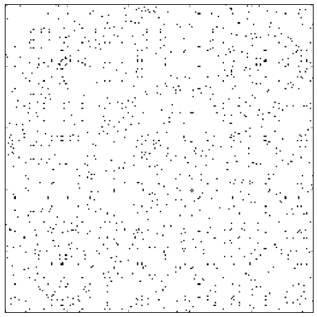
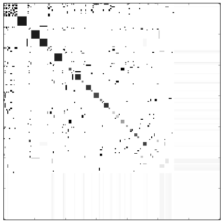
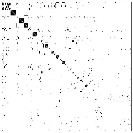
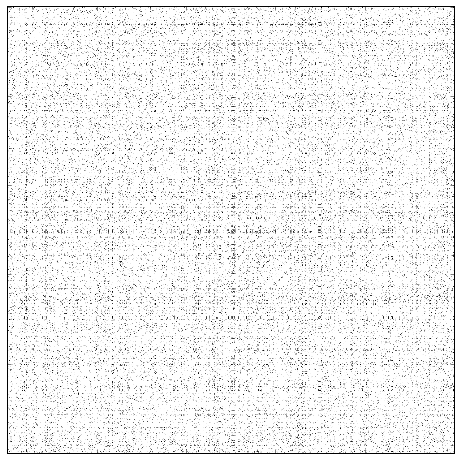
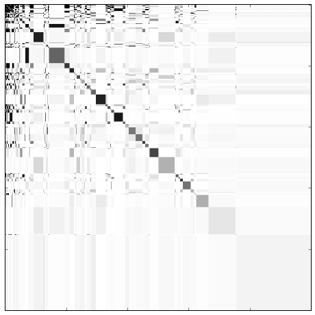
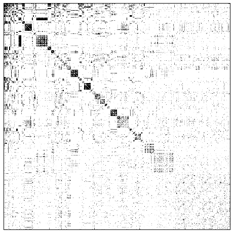
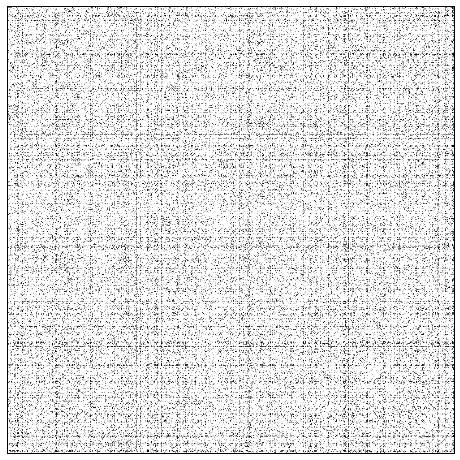
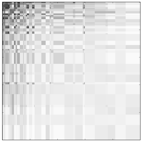
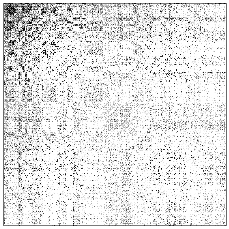
We examine three real-world social network datasets, considering a denser subgraph constructed by taking the top $K$ highest-degree vertices and the edges between them, for reasons we describe below. We randomized the order of the vertices for each graph before running the ISFE algorithm, which we present in Figure 8.

Many real-world networks, such as those arising from co-authorship, social interactions, etc., are not well-modeled as exchangeable graphs, as they tend to exhibit power-law degree distributions, “small-world” phenomena such as short path lengths, and other properties that generally hold only for sparse sequences of graphs (having $o(n^{2})$ edges among $n$ vertices, which is not possible for non-empty exchangeable graphs). For a detailed discussion, see Orbanz and Roy (2015, §VII).

One approach to modeling sparse graphs using graphons is the Bollobás–Janson–Riordan model (Bollobás et al., 2007), where edges are independently deleted from an exchangeable graph to achieve the desired edge density. Although this process does not exhibit many of the above real-world phenomena (Orbanz and Roy, 2015, Example VII.4), the behavior of graphon estimators on graphs sampled in this way has been considered (Bickel et al., 2011; Wolfe and Olhede, 2013).

Here we avoid these issues to some degree by considering a denser subset of the original graph.

1. NIPS co-authorship dataset (Globerson et al., 2007): This dataset is an undirected network of co-authorships in the NIPS conference from Proceedings 1–12, with 2,037 vertices and 1,740 edges. We choose $K=234$ for the denser subset, which has been studied in other work (Miller et al., 2009; Palla et al., 2012). For the ISFE parameters, we set $T=8,\ell=95$, initializing it with a $90$ cluster $k$-means partition.

2. ca-AstroPh co-authorship dataset (Newman, 2001): This dataset is an undirected network of co-authorships between scientists posting pre-prints on the Astrophysics E-Print Archive between Jan 1, 1995 and December 31, 1999 with 18,772 vertices and 396,160 edges. We choose $K=1000$, and set the ISFE parameters to $T=8$, $\ell=160$, initializing it with a $150$ cluster partition from $k$-means.

3. Epinions dataset (Richardson et al., 2003): This dataset is a who-trusts-whom network of Epinions.com with 75,879 vertices, 508,837 edges. We work with the undirected graph obtained by symmetrizing the original undirected graph, choose $K=1000$, and set $T=8$, $\ell=40$, initializing it with a $35$ cluster partition from $k$-means.

References

- Airoldi et al. (2013) E. M. Airoldi, T. B. Costa, and S. H. Chan. Stochastic blockmodel approximation of a graphon: Theory and consistent estimation. In Adv. Neural Inform. Process. Syst. (NIPS) 26, pages 692–700, 2013.
- Aldous (1981) D. J. Aldous. Representations for partially exchangeable arrays of random variables. J. Multivariate Anal., 11(4):581–598, 1981.
- Amini and Levina (2014) A. A. Amini and E. Levina. On semidefinite relaxations for the block model. ArXiv e-print 1406.5647, 2014.
- Austin (2008) T. Austin. On exchangeable random variables and the statistics of large graphs and hypergraphs. Probab. Surv., 5:80–145, 2008.
- Bickel and Chen (2009) P. J. Bickel and A. Chen. A nonparametric view of network models and Newman-Girvan and other modularities. Proc. Natl. Acad. Sci. USA, 106(50):21068–21073, 2009.
- Bickel et al. (2011) P. J. Bickel, A. Chen, and E. Levina. The method of moments and degree distributions for network models. Ann. Statist., 39(5):2280–2301, 2011.
- Bollobás et al. (2007) B. Bollobás, S. Janson, and O. Riordan. The phase transition in inhomogeneous random graphs. Random Structures Algorithms, 31(1):3–122, 2007.
- Chan and Airoldi (2014) S. H. Chan and E. Airoldi. A consistent histogram estimator for exchangeable graph models. In Proc. 31st Int. Conf. Mach. Learn. (ICML), pages 208–216, 2014.
- Chatterjee (2014) S. Chatterjee. Matrix estimation by universal singular value thresholding. ArXiv e-print 1212.1247v6, 2014.
- Choi and Wolfe (2014) D. Choi and P. J. Wolfe. Co-clustering separately exchangeable network data. Ann. Statist., 42(1):29–63, 2014.
- Diaconis and Janson (2008) P. Diaconis and S. Janson. Graph limits and exchangeable random graphs. Rend. Mat. Appl. (7), 28(1):33–61, 2008.
- Frieze and Kannan (1999a) A. Frieze and R. Kannan. A simple algorithm for constructing Szemerédi’s regularity partition. Electron. J. Combin., 6:R17, 7 pp., 1999a.
- Frieze and Kannan (1999b) A. Frieze and R. Kannan. Quick approximation to matrices and applications. Combinatorica, 19(2):175–220, 1999b.
- Gao et al. (2014) C. Gao, Y. Lu, and H. H. Zhou. Rate-optimal graphon estimation. ArXiv e-print 1410.5837, 2014.
- Girvan and Newman (2002) M. Girvan and M. E. J. Newman. Community structure in social and biological networks. Proc. Natl. Acad. Sci. USA, 99(12):7821–7826, 2002.
- Globerson et al. (2007) A. Globerson, G. Chechik, F. Pereira, and N. Tishby. Euclidean embedding of co-occurrence data. J. Mach. Learn. Res., 8:2265–2295, 2007.
- Hoff (2007) P. Hoff. Modeling homophily and stochastic equivalence in symmetric relational data. In Adv. Neural Inform. Process. Syst. (NIPS) 20, pages 657–664, 2007.
- Hoff et al. (2002) P. D. Hoff, A. E. Raftery, and M. S. Handcock. Latent space approaches to social network analysis. J. Amer. Statist. Assoc., 97(460):1090–1098, 2002.
- Holland et al. (1983) P. W. Holland, K. B. Laskey, and S. Leinhardt. Stochastic blockmodels: first steps. Social Networks, 5(2):109–137, 1983.
- Hoover (1979) D. N. Hoover. Relations on probability spaces and arrays of random variables. Preprint, Institute for Advanced Study, Princeton, NJ, 1979.
- Janson (2013) S. Janson. Graphons, cut norm and distance, couplings and rearrangements, volume 4 of New York J. Math. Monographs. Univ. at Albany, State Univ. of New York, Albany, NY, 2013.
- Kallenberg (1999) O. Kallenberg. Multivariate sampling and the estimation problem for exchangeable arrays. J. Theoret. Probab., 12(3):859–883, 1999.
- Kallenberg (2005) O. Kallenberg. Probabilistic symmetries and invariance principles. Probab. Applic. Springer, New York, 2005.
- Kemp et al. (2006) C. Kemp, J. B. Tenenbaum, T. L. Griffiths, T. Yamada, and N. Ueda. Learning systems of concepts with an infinite relational model. In Proc. 21st Nat. Conf. Artificial Intelligence (AAAI-06), 2006.
- Lloyd et al. (2012) J. R. Lloyd, P. Orbanz, Z. Ghahramani, and D. M. Roy. Random function priors for exchangeable arrays with applications to graphs and relational data. In Adv. Neural Inform. Process. Syst. (NIPS) 25, pages 1007–1015, 2012.
- Lovász (2012) L. Lovász. Large networks and graph limits, volume 60 of American Math. Soc. Colloq. Publ. American Math. Soc., Providence, RI, 2012.
- MacQueen (1967) J. MacQueen. Some methods for classification and analysis of multivariate observations. In Proc. Fifth Berkeley Sympos. Math. Statist. and Probability (Berkeley, Calif., 1965/66), pages Vol. I: Statistics, pp. 281–297. Univ. California Press, Berkeley, Calif., 1967.
- Miller et al. (2009) K. T. Miller, T. L. Griffiths, and M. I. Jordan. Nonparametric latent feature models for link prediction. In Adv. Neural Inform. Process. Syst. (NIPS) 22, pages 1276–1284, 2009.
- Newman (2001) M. E. J. Newman. The structure of scientific collaboration networks. Proc. Natl. Acad. Sci. USA, 98(2):404–409, 2001.
- Olhede and Wolfe (2014) S. C. Olhede and P. J. Wolfe. Network histograms and universality of blockmodel approximation. Proc. Natl. Acad. Sci. USA, 2014.
- Orbanz and Roy (2015) P. Orbanz and D. M. Roy. Bayesian models of graphs, arrays and other exchangeable random structures. IEEE Trans. Pattern Anal. Mach. Intell., 37(2):437–461, 2015.
- Palla et al. (2012) K. Palla, D. A. Knowles, and Z. Ghahramani. An infinite latent attribute model for network data. In Proc. 29th Int. Conf. Mach. Learn. (ICML), 2012.
- Pedregosa et al. (2011) F. Pedregosa, G. Varoquaux, A. Gramfort, et al. Scikit-learn: Machine learning in Python. J. Mach. Learn. Res., 12:2825–2830, 2011.
- Richardson et al. (2003) M. Richardson, R. Agrawal, and P. Domingos. Trust management for the semantic web. In The Semantic Web - ISWC 2003, volume 2870 of Lecture Notes Comput. Sci., pages 351–368. Springer, 2003.
- Roy and Teh (2008) D. M. Roy and Y. W. Teh. The Mondrian process. In Adv. Neural Inform. Process. Syst. (NIPS) 21, pages 1377–1384, 2008.
- Tsybakov (2009) A. B. Tsybakov. Introduction to nonparametric estimation. Springer Ser. Statist. Springer, New York, 2009.
- Ward, Jr. (1963) J. H. Ward, Jr. Hierarchical grouping to optimize an objective function. J. Amer. Statist. Assoc., 58:236–244, 1963.
- Wolfe and Olhede (2013) P. J. Wolfe and S. C. Olhede. Nonparametric graphon estimation. ArXiv e-print 1309.5936, 2013.
- Yang et al. (2014) J. Yang, C. Han, and E. Airoldi. Nonparametric estimation and testing of exchangeable graph models. In Proc. 17th Int. Conf. Artificial Intelligence Statist. (AISTATS), pages 1060–1067, 2014.