Fast Bundle-Level Type Methods for unconstrained and ball-constrained convex optimizationthanks: December, 2014. This research was partially supported by NSF grants CMMI-1254446, DMS-1319050, and ONR grant N00014-13-1-0036.

Yunmei Chen Department of Mathematics, University of Florida (yun@math.ufl.edu).    Guanghui Lan Department of Industrial and System Engineering, University of Florida (glan@ise.ufl.edu)    Yuyuan Ouyang Department of Industrial and System Engineering, University of Florida (ouyang@ufl.edu)    Wei Zhang Department of Mathematics, University of Florida (weizhang657@ufl.edu)
Abstract

It has been shown in [14] that the accelerated prox-level (APL) method and its variant, the uniform smoothing level (USL) method, have optimal iteration complexity for solving black-box and structured convex programming problems without requiring the input of any smoothness information. However, these algorithms require the assumption on the boundedness of the feasible set and their efficiency relies on the solutions of two involved subproblems. These hindered the applicability of these algorithms in solving large-scale and unconstrained optimization problems. In this paper, we first present a generic algorithmic framework to extend these uniformly optimal level methods for solving unconstrained problems. Moreover, we introduce two new variants of level methods, i.e., the fast APL (FAPL) method and the fast USL (FUSL) method, for solving large scale black-box and structured convex programming problems respectively. Both FAPL and FUSL enjoy the same optimal iteration complexity as APL and USL, while the number of subproblems in each iteration is reduced from two to one. Moreover, we present an exact method to solve the only subproblem for these algorithms. As a result, the proposed FAPL and FUSL methods have improved the performance of the APL and USL in practice significantly in terms of both computational time and solution quality. Our numerical results on solving some large-scale least square problems and total variation based image reconstruction have shown great advantages of these new bundle-level type methods over APL, USL, and some other state-of-the-art first-order methods.

Keywords: convex programming, first-order, optimal method, bundle-level type method, total variation, image reconstruction

AMS 2000 subject classification: 90C25, 90C06, 90C22, 49M37

1 Introduction

Given a convex function f:n:𝑓superscript𝑛f:\mathbb{R}^{n}\rightarrow\mathbb{R}, the main problem of interest in this paper is:

f:=minxnf(x).assignsuperscript𝑓subscript𝑥superscript𝑛𝑓𝑥f^{\ast}:=\min_{x\in\mathbb{R}^{n}}f(x). (1.1)

Throughout this paper, we assume that the solution set Xsuperscript𝑋X^{\ast} of (1.1) is nonempty. Moreover, denoting

x:=argminx{x¯x:xX}andD:=x¯xx^{\ast}:={\rm argmin}_{x}\{\|\overline{x}-x\|:x\in X^{\ast}\}\ \ \mbox{and}\ \ \ D^{\ast}:=\|\overline{x}-x^{\ast}\| (1.2)

for a given initial point x¯n¯𝑥superscript𝑛\overline{x}\in\mathbb{R}^{n}, we assume in the black-box setting that for all closed sets

ΩB(x¯,4D):={xn:xx¯4D},Ω𝐵¯𝑥4superscript𝐷assignconditional-set𝑥superscript𝑛norm𝑥¯𝑥4superscript𝐷\Omega\subseteq B(\overline{x},4D^{\ast}):=\left\{x\in\mathbb{R}^{n}:\|x-\overline{x}\|\leq 4D^{\ast}\right\}, (1.3)

there exists M(Ω)>0𝑀Ω0M(\Omega)>0 and ρ(Ω)[0,1]𝜌Ω01\rho(\Omega)\in[0,1], such that111Observe that this assumption is weaker than requiring (1.4) holds for any x,yn𝑥𝑦superscript𝑛x,y\in\mathbb{R}^{n}.

f(y)f(x)f(x),yxM(Ω)1+ρ(Ω)yx1+ρ(Ω),x,yΩ.formulae-sequence𝑓𝑦𝑓𝑥superscript𝑓𝑥𝑦𝑥𝑀Ω1𝜌Ωsuperscriptnorm𝑦𝑥1𝜌Ωfor-all𝑥𝑦Ωf(y)-f(x)-\left\langle f^{\prime}(x),y-x\right\rangle\leq\frac{M(\Omega)}{1+\rho(\Omega)}\|y-x\|^{1+\rho(\Omega)},\ \ \forall x,y\in\Omega. (1.4)

Here \|\cdot\| denotes the Euclidean norm, and f(x)f(x)superscript𝑓𝑥𝑓𝑥f^{\prime}(x)\in\partial f(x), where f(x)𝑓𝑥\partial f(x) denotes the subdifferential of f𝑓f at xΩ𝑥Ωx\in\Omega. Clearly, the above assumption on f()𝑓f(\cdot) covers non-smooth (ρ(Ω)=0𝜌Ω0\rho(\Omega)=0), smooth (ρ(Ω)=1𝜌Ω1\rho(\Omega)=1) and weakly smooth (0<ρ(Ω)<10𝜌Ω10<\rho(\Omega)<1) functions.

Our main goal in this paper is to develop a bundle-level method that is able to compute an approximate solution to problem (1.1), with uniformly optimal iteration complexity for non-smooth, smooth and weakly smooth objective functions (see [14]). Here, the iteration complexity is described by the number of evaluations of subgradients/gradients of f𝑓f. In addition, we aim to design the bundle-level method so that its computational cost in each iteration is small, in order to improve its practical performance. Let us start by reviewing a few existing bundle-level methods.

1.1 Cutting plane, bundle and bundle-level methods

The bundle-level method originated from the well-known Kelley’s cutting-plane method in 1960 [8]. Consider the convex programming (CP) problem of

minxXf(x),subscript𝑥𝑋𝑓𝑥\displaystyle\min_{x\in X}f(x), (1.5)

where X𝑋X is a compact convex set and f𝑓f is a closed convex function. The fundamental idea of the cutting plane method is to generate a sequence of piecewise linear functions to approximate f𝑓f in X𝑋X. In particular, given x1,x2,,xkXsubscript𝑥1subscript𝑥2subscript𝑥𝑘𝑋x_{1},x_{2},\ldots,x_{k}\in X, we approximate f𝑓f by

mk(x):=max{h(xi,x),1ik},assignsubscript𝑚𝑘𝑥subscript𝑥𝑖𝑥1𝑖𝑘m_{k}(x):=\max\{h(x_{i},x),1\leq i\leq k\}, (1.6)

and compute the iterates xk+1subscript𝑥𝑘1x_{k+1} by:

xk+1ArgminxXmk(x),subscript𝑥𝑘1subscriptArgmin𝑥𝑋subscript𝑚𝑘𝑥x_{k+1}\in{\rm Argmin}_{x\in X}m_{k}(x), (1.7)

where

h(z,x):=f(z)+f(z),xz.assign𝑧𝑥𝑓𝑧superscript𝑓𝑧𝑥𝑧h(z,x):=f(z)+\left\langle f^{\prime}(z),x-z\right\rangle. (1.8)

Clearly, the functions misubscript𝑚𝑖m_{i}, i=1,2,𝑖12i=1,2,\ldots, satisfy mi(x)mi+1(x)f(x)subscript𝑚𝑖𝑥subscript𝑚𝑖1𝑥𝑓𝑥m_{i}(x)\leq m_{i+1}(x)\leq f(x) for any xX𝑥𝑋x\in X, and are identical to f𝑓f at those search points xisubscript𝑥𝑖x_{i}, i=1,,k𝑖1𝑘i=1,\ldots,k. However, the inaccuracy and instability of the piecewise linear approximation mksubscript𝑚𝑘m_{k} over the whole feasible set X𝑋X may affect the selection of new iterates, and the above scheme converges slowly both theoretically and practically [18, 20]. Some important improvements of Kelley’s method have been made in 1990s under the name of bundle methods (see, e.g., [9, 10, 16]). In particular, by incorporating the level sets into Kelley’s method, Lemaréchal, Nemirovskii and Nesterov [16] proposed in 1995 the classic bundle-level (BL) method by performing a series of projections over the approximate level sets.

Given x1,x2,,xksubscript𝑥1subscript𝑥2subscript𝑥𝑘x_{1},x_{2},\ldots,x_{k}, the basic BL iteration consists of the following three steps:

  • a)

    Set f¯k:=min{f(xi),1ik}assignsubscript¯𝑓𝑘𝑓subscript𝑥𝑖1𝑖𝑘\overline{f}_{k}:=\min\{f(x_{i}),1\leq i\leq k\} and compute a lower bound on fsuperscript𝑓f^{*} by f¯k=minxXmk(x).subscript¯𝑓𝑘subscript𝑥𝑋subscript𝑚𝑘𝑥\underline{\smash{f}}_{k}=\min_{x\in X}m_{k}(x).

  • b)

    Set the level lk=βf¯k+(1β)f¯ksubscript𝑙𝑘𝛽subscript¯𝑓𝑘1𝛽subscript¯𝑓𝑘l_{k}=\beta\underline{\smash{f}}_{k}+(1-\beta)\overline{f}_{k} for some β(0,1)𝛽01\beta\in(0,1).

  • c)

    Set Xk:={xX:mk(x)lk}assignsubscript𝑋𝑘conditional-set𝑥𝑋subscript𝑚𝑘𝑥subscript𝑙𝑘X_{k}:=\{x\in X:m_{k}(x)\leq l_{k}\} and determine the new iterate

    xk+1=argminxXkxxk2.subscript𝑥𝑘1subscriptargmin𝑥subscript𝑋𝑘superscriptnorm𝑥subscript𝑥𝑘2x_{k+1}={\rm argmin}_{x\in X_{k}}\|x-x_{k}\|^{2}. (1.9)

In the BL method, the localizer Xksubscript𝑋𝑘X_{k} is used to approximate the level set Lk:={x:f(x)lk}assignsubscript𝐿𝑘conditional-set𝑥𝑓𝑥subscript𝑙𝑘L_{k}:=\{x:f(x)\leq l_{k}\}, because the projection over Lksubscript𝐿𝑘L_{k} is often too difficult to compute. Intuitively, as k𝑘k increases, the value of lksubscript𝑙𝑘l_{k} will converge to fsuperscript𝑓f^{*}, and consequently both Lksubscript𝐿𝑘L_{k} and Xksubscript𝑋𝑘X_{k} will converge to the set of optimal solutions for problem (1.5). It is shown in [16] the number of BL iterations required to find an ϵitalic-ϵ\epsilon-solution of (1.5), i.e., a point x^X^𝑥𝑋\hat{x}\in X s.t. f(x^)fϵ𝑓^𝑥superscript𝑓italic-ϵf(\hat{x})-f^{*}\leq\epsilon, can be bounded by 𝒪(1/ϵ2)𝒪1superscriptitalic-ϵ2{\cal O}(1/\epsilon^{2}), which is optimal for general nonsmooth convex optimization.

Observe that for the above BL methods, the localizer Xksubscript𝑋𝑘X_{k} accumulates constraints, and hence that the subproblem in step c) becomes more and more expensive to solve. In order to overcome this difficulty, some restricted memory BL algorithms have been developed in [10, 3]. In particular, Ben-Tal and Nemirovski [3] introduced the non-Euclidean restricted memory level (NERML) method, in which the number of extra linear constraints in Xksubscript𝑋𝑘X_{k} can be as small as 111 or 222, without affecting the optimal iteration complexity. Moreover, the objective function 2\|\cdot\|^{2} in (1.9) is replaced by a general Bregman distance d()𝑑d(\cdot) for exploiting the geometry of the feasible set X𝑋X. NERML is often regarded as state-of-the-art for large-scale nonsmooth convex optimization as it substantially outperforms subgradient type methods in practice. Some more recent development of inexact proximal bundle methods and BL methods could be found in [27, 23, 22, 26, 12, 11, 7, 13].

1.2 Accelerated bundle-level type methods

While the classic BL method was optimal for solving nonsmooth CP problems only, Lan [14] recently significantly generalized this method so that they can optimally solve any black-box CP problems, including non-smooth, smooth and weakly smooth CP problems. In particular, for problem (1.5) with compact feasible set X𝑋X, the two new BL methods proposed in [14], i.e., the accelerated bundle-level(ABL) and accelerated prox-level(APL) methods, can solve these problems optimally without requiring any information on problem parameters. The ABL method can be viewed as an accelerated version of the classic BL method. Same as the classic BL method, the lower bound on fsuperscript𝑓f^{*} is estimated from the cutting plane model mksubscript𝑚𝑘m_{k} in (1.6), the upper bound on fsuperscript𝑓f^{*} is given by the best objective value found so far, and the prox-center is updated by (1.9). The novelty of the ABL method exists in that three different sequences, i.e, {xkl},{xk}superscriptsubscript𝑥𝑘𝑙subscript𝑥𝑘\{x_{k}^{l}\},\{x_{k}\} and {xku}superscriptsubscript𝑥𝑘𝑢\{x_{k}^{u}\}, are used for updating lower bound, prox-center, and upper bound respectively, which leads to its accelerated iteration complexity for smooth and weakly smooth problems. The APL method is a more practical, restricted memory version of the ABL method, which can also employ non-Euclidean prox-functions to explore the geometry of the feasible set X𝑋X.

We now provide a brief description of the APL method. This method consists of multiple phases, and each phase calls a gap reduction procedure to reduce the gap between the lower and upper bounds on fsuperscript𝑓f^{*} by a constant factor. More specifically, at phase s𝑠s, given the initial lower bound lbssubscriptlb𝑠{\rm lb}_{s} and upper bound ubssubscriptub𝑠{\rm ub}_{s}, the APL gap reduction procedure sets f¯0=lbs,f¯0=ubs,l=βlbs+(1β)ubsformulae-sequencesubscript¯𝑓0subscriptlb𝑠formulae-sequencesubscript¯𝑓0subscriptub𝑠𝑙𝛽subscriptlb𝑠1𝛽subscriptub𝑠\underline{\smash{f}}_{0}={\rm lb}_{s},\overline{f}_{0}={\rm ub}_{s},l=\beta\cdot{\rm lb}_{s}+(1-\beta){\rm ub}_{s}, and iteratively performs the following steps.

  • a)

    Set xkl=(1αk)xk1u+αkxk1superscriptsubscript𝑥𝑘𝑙1subscript𝛼𝑘superscriptsubscript𝑥𝑘1𝑢subscript𝛼𝑘subscript𝑥𝑘1x_{k}^{l}=(1-\alpha_{k})x_{k-1}^{u}+\alpha_{k}x_{k-1} and f¯k:=max{f¯k1,min{l,h¯k}}assignsubscript¯𝑓𝑘subscript¯𝑓𝑘1𝑙subscript¯𝑘\underline{\smash{f}}_{k}:=\max\{\underline{\smash{f}}_{k-1},\min\{l,\underline{\smash{h}}_{k}\}\}, where

    h¯k:=minxXk1h(xkl,x).assignsubscript¯𝑘subscript𝑥subscript𝑋𝑘1superscriptsubscript𝑥𝑘𝑙𝑥\underline{\smash{h}}_{k}:=\min_{x\in X_{k-1}}h(x_{k}^{l},x). (1.10)
  • b)

    Update the prox-center xksubscript𝑥𝑘x_{k} by

    xk=argminxX¯kd(x),subscript𝑥𝑘subscriptargmin𝑥subscript¯𝑋𝑘𝑑𝑥x_{k}={\rm argmin}_{x\in\underline{\smash{X}}_{k}}d(x), (1.11)

    where X¯k:={xXk1:h(xkl,x)l}assignsubscript¯𝑋𝑘conditional-set𝑥subscript𝑋𝑘1superscriptsubscript𝑥𝑘𝑙𝑥𝑙\underline{\smash{X}}_{k}:=\{x\in X_{k-1}:h(x_{k}^{l},x)\leq l\}.

  • c)

    Set f¯k=min{f¯k1,f(x~k)}subscript¯𝑓𝑘subscript¯𝑓𝑘1𝑓subscript~𝑥𝑘\overline{f}_{k}=\min\{\overline{f}_{k-1},f(\tilde{x}_{k})\}, where x~ku=αkxk+(1αk)xk1usuperscriptsubscript~𝑥𝑘𝑢subscript𝛼𝑘subscript𝑥𝑘1subscript𝛼𝑘superscriptsubscript𝑥𝑘1𝑢\tilde{x}_{k}^{u}=\alpha_{k}x_{k}+(1-\alpha_{k})x_{k-1}^{u}, and xkusuperscriptsubscript𝑥𝑘𝑢x_{k}^{u} is chosen as either x~kusuperscriptsubscript~𝑥𝑘𝑢\tilde{x}_{k}^{u} or xk1usuperscriptsubscript𝑥𝑘1𝑢x_{k-1}^{u} such that f(xku)=f¯k𝑓superscriptsubscript𝑥𝑘𝑢subscript¯𝑓𝑘f(x_{k}^{u})=\overline{f}_{k}.

  • d)

    Choose Xksubscript𝑋𝑘X_{k} such that X¯kXkX¯ksubscript¯𝑋𝑘subscript𝑋𝑘subscript¯𝑋𝑘\underline{\smash{X}}_{k}\subseteq X_{k}\subseteq\overline{X}_{k}, where X¯k:={xX:d(xk),xxk0}.assignsubscript¯𝑋𝑘conditional-set𝑥𝑋𝑑subscript𝑥𝑘𝑥subscript𝑥𝑘0\overline{X}_{k}:=\{x\in X:\left\langle\nabla d(x_{k}),x-x_{k}\right\rangle\geq 0\}.

Here d()𝑑\nabla d(\cdot) denotes the gradient of d()𝑑d(\cdot). Observe that the parameters αksubscript𝛼𝑘\alpha_{k} and β𝛽\beta are fixed a priori, and do not depend on any problem parameters. Moreover, the localizer Xksubscript𝑋𝑘X_{k} is chosen between X¯ksubscript¯𝑋𝑘\underline{\smash{X}}_{k} and X¯ksubscript¯𝑋𝑘\overline{X}_{k}, so that the numbers of linear constraints in the two subproblems (1.10) and (1.11) can be fully controlled. It is shown in [14] that for problem (1.5) with compact feasible set X𝑋X, the APL method achieves the optimal iteration complexity for any smooth, weakly smooth and non-smooth convex functions. Moreover, by incorporating Nesterov’s smoothing technique [21] into the APL method, Lan also presented in [14] the uniform smoothing level (USL) method which can achieve the optimal complexity for solving an important class of nonsmooth structured saddle point (SP) problems without requiring the input of any problem parameters (see Subsection 3.2 for more details).

1.3 Contribution of this paper

One crucial problem associated with most existing BL type methods, including APL and USL, is that each phase of these algorithms involves solving two optimization problems; first a linear programing problem to compute the lower bound, and then a constrained quadratic programing problem to update the prox-center or new iterate. In fact, the efficiency of these algorithms relies on the solutions of the two involved subproblems (1.10) and (1.11), and the latter one is often more complicated than the projection subproblem in the gradient projection type methods. Moreover, most existing BL type methods require the assumption that the feasible set is bounded due to the following two reasons. Firstly, the feasible set has to be bounded to compute a meaningful lower bound by solving the aforementioned linear programing problem. Secondly, the convergence analysis of limited memory BL type methods (e.g., NERML, APL, and USL) relies on the assumption that the feasible set is compact. These issues have significantly hindered the applicability of existing BL type methods. Our contribution in this paper mainly consists of the following three aspects.

Firstly, we propose a novel bundle-level framework for unconstrained CP problems. The proposed framework solves unconstrained CP problems through solutions to a series of ball-constrained CPs. In particular, if there exists a uniformly optimal method (e.g., the APL and USL methods) that solves ball-constrained black-box or structured CPs, then the proposed algorithm solves unconstrained black-box or structured CPs with optimal complexity without requiring the input of any problem parameters as well. To the best of our knowledge, this is the first time in the literature that the complexity analysis has been performed for BL type methods to solve unconstrained CP problems (see Sections 3.2 and 3.3 in [24] for more details).

Secondly, in order to solve ball-constrained CPs, we propose two greatly simplified BL type methods, namely the FAPL and FUSL methods, which achieve the same optimal iteration complexity as the APL and USL methods respectively, and maintain all the nice features of those methods, but has greatly reduced computational cost per iteration. Such improvement has been obtained by the reduction and simplification of the subproblems that have to be solved in the APL and USL methods. More specifically, we show that the linear optimization subproblem for computing the lower bound can be eliminated and that the ball constraint can be removed from the quadratic subproblem by properly choosing the prox-functions. We also generalize both FAPL and FUSL methods for solving strongly convex optimization problems and show that they can achieve the optimal iteration complexity bounds.

Thirdly, we introduce a simple exact approach to solve the only subproblem in our algorithms. As mentioned earlier, the accuracy of the solutions to the subproblems is essential for the efficiency of all these BL type methods mentioned in Sections 1.1 and 1.2. By incorporating the proposed exact approach to solve the only subproblem in our algorithm, the accuracy of the FAPL and FUSL methods is significantly increased and the total number of the iterations required to compute an ϵitalic-ϵ\epsilon-solution is greatly decreased comparing with the original APL and USL methods and other first order methods. Also when the number of linear constraints is fixed and small, the computational cost for solving the only subproblem only linearly depends on the dimension of the problem, since the cost for computing the vector inner product will dominate that for solving a few auxiliary linear systems. This feature is very important for solving large-scale CP problems.

Finally, we present very promising numerical results for these new FAPL and FUSL methods applied to solve large-scale least square problems and total-variation based image reconstruction problems. These algorithms significantly outperform other BL type methods, gradient type methods, and even the powerful MATLAB solver for linear systems, especially when the dimension and/or the Lipschitz constant of the problem is large.

It should be noted that there exist some variants of bundle-level methods [4, 7, 2] for solving nonsmooth CP problems in which the computation of the subproblem to update the lower bound f¯ksubscript¯𝑓𝑘\underline{\smash{f}}_{k} is skipped, so that the feasible set X𝑋X is allowed to be unbounded. In each iteration, these methods apply a level feasibility check recursively in order to find a proper level lksubscript𝑙𝑘l_{k} and the associated level set Xksubscript𝑋𝑘X_{k}, and update f¯ksubscript¯𝑓𝑘\underline{\smash{f}}_{k} to lksubscript𝑙𝑘l_{k} if the level set associated with lksubscript𝑙𝑘l_{k} is empty. However, in these methods, repeatedly checking the emptiness of level sets associated with varied levels in each iteration may be very costly in practice, especially when the linear constraints in the level sets accumulate. Also, if the feasible set X=n𝑋superscript𝑛X=\mathbb{R}^{n}, then for any chosen level, the corresponding level set consisting of linear constraints is unlikely to be empty, which would result in the inefficiency for updating the lower bound. In [2], an alternative for updating the lower bound (or increasing the level) is introduced by comparing the distances from stability center to the newly generated iterate and the solution set. This approach requires some prior knowledge about the distance to the solution set, and a rough estimate for that may lead to incorrect lower bounds and improper choices of levels.

1.4 Organization of the paper

The paper is organized as follows. In Section 2, we present a general scheme to extend the optimal BL type methods for unconstrained convex optimization. In Section 3, the new FAPL and FUSL methods are proposed followed by their convergence analysis, then an exact approach is introduced to solve the subproblem in these algorithms. We also extend the FAPL and FUSL methods to strongly convex CP and structured CP problems in Section 4, following some unpublished developments by Lan in [15]. The applications and promising numerical results are presented in Section 5.

2 Solving unconstrained CP problems through ball-constrained CP

Our goal in this section is to present a generic algorithmic framework to extend the uniformly optimal constrained BL algorithms in [14] for solving unconstrained problems.

Given x¯n,R>0,ϵ>0formulae-sequence¯𝑥superscript𝑛formulae-sequence𝑅0italic-ϵ0\overline{x}\in\mathbb{R}^{n},R>0,\epsilon>0, let us assume that there exists a first-order algorithm, denoted by 𝒜(x¯,R,ϵ)𝒜¯𝑥𝑅italic-ϵ\mathcal{A}(\overline{x},R,\epsilon), which can find an ϵitalic-ϵ\epsilon-solution of

fx¯,R:=minxB(x¯,R)f(x),assignsubscriptsuperscript𝑓¯𝑥𝑅subscript𝑥𝐵¯𝑥𝑅𝑓𝑥\displaystyle f^{*}_{\overline{x},R}:=\min_{x\in B(\overline{x},R)}f(x), (2.1)

where B(x¯,R)𝐵¯𝑥𝑅B(\overline{x},R) is defined in (1.3). In other words, we assume that each call to 𝒜(x¯,R,ϵ)𝒜¯𝑥𝑅italic-ϵ\mathcal{A}(\overline{x},R,\epsilon) will compute a point zB(x¯,R)𝑧𝐵¯𝑥𝑅z\in B(\overline{x},R) such that f(z)fx¯,Rϵ𝑓𝑧subscriptsuperscript𝑓¯𝑥𝑅italic-ϵf(z)-f^{*}_{\overline{x},R}\leq\epsilon. Moreover, throughout this section, we assume that the iteration complexity associated with 𝒜(x¯,R,ϵ)𝒜¯𝑥𝑅italic-ϵ\mathcal{A}(\overline{x},R,\epsilon) is given by

Nx¯,R,ϵ:=C1(x¯,R,f)Rα1ϵβ1+C2(x¯,R,f)Rα2ϵβ2,assignsubscript𝑁¯𝑥𝑅italic-ϵsubscript𝐶1¯𝑥𝑅𝑓superscript𝑅subscript𝛼1superscriptitalic-ϵsubscript𝛽1subscript𝐶2¯𝑥𝑅𝑓superscript𝑅subscript𝛼2superscriptitalic-ϵsubscript𝛽2\displaystyle N_{\overline{x},R,\epsilon}:=\frac{C_{1}(\overline{x},R,f)R^{\alpha_{1}}}{\epsilon^{\beta_{1}}}+\frac{C_{2}(\overline{x},R,f)R^{\alpha_{2}}}{\epsilon^{\beta_{2}}}, (2.2)

where α1β1>0,α2β2>0formulae-sequencesubscript𝛼1subscript𝛽10subscript𝛼2subscript𝛽20\alpha_{1}\geq\beta_{1}>0,\alpha_{2}\geq\beta_{2}>0 and C1(x¯,R,f),C2(x¯,R,f)subscript𝐶1¯𝑥𝑅𝑓subscript𝐶2¯𝑥𝑅𝑓C_{1}(\overline{x},R,f),C_{2}(\overline{x},R,f) are some constants that depend on f𝑓f in (2.1). For example, if f𝑓f is a smooth convex function, f𝑓\nabla f is Lipschitz continuous in nsuperscript𝑛\mathbb{R}^{n} with constant L𝐿L, i.e., (1.4) holds with ρ(n)=1𝜌superscript𝑛1\rho(\mathbb{R}^{n})=1 and M(n)=L𝑀superscript𝑛𝐿M(\mathbb{R}^{n})=L, and we apply the APL method to (2.1), then we have only one term with α1=1subscript𝛼11\alpha_{1}=1, β1=1/2subscript𝛽112\beta_{1}=1/2, and C1(x¯,R,f)=cLsubscript𝐶1¯𝑥𝑅𝑓𝑐𝐿C_{1}(\overline{x},R,f)=cL in (2.2), where c𝑐c is a universal constant. Observe that the two complexity terms in (2.2) will be useful for analyzing some structured CP problems in Section 3.2. It should also be noted that a more accurate estimate of C1(x¯,R,f)subscript𝐶1¯𝑥𝑅𝑓C_{1}(\overline{x},R,f) is cM(B(x¯,R))𝑐𝑀𝐵¯𝑥𝑅cM(B(\overline{x},R)), since the Lipschitz constant L=M(n)𝐿𝑀superscript𝑛L=M(\mathbb{R}^{n}) throughout nsuperscript𝑛\mathbb{R}^{n} is larger than or equal to the local Lipschitz constant in B(x¯,R)𝐵¯𝑥𝑅B(\overline{x},R).

By utilizing the aforementioned ball-constrained CP algorithm and a novel guess and check procedure, we present a bundle-level type algorithm for unconstrained convex optimiations as follows.

Algorithm 1 Bundle-level type methods for unconstrained CP problems

Choose initial estimation r0x¯xsubscript𝑟0norm¯𝑥superscript𝑥r_{0}\leq\|\overline{x}-x^{\ast}\| and compute the initial gap Δ0:=f(x¯)minxB(x¯,r0)h(x¯,x)assignsubscriptΔ0𝑓¯𝑥subscript𝑥𝐵¯𝑥subscript𝑟0¯𝑥𝑥\Delta_{0}:=f(\overline{x})-\min_{x\in B(\overline{x},r_{0})}h(\overline{x},x).

For k=0,1,2,𝑘012k=0,1,2,\ldots,

1. Set x¯k=𝒜(x¯,rk,Δk)superscriptsubscript¯𝑥𝑘𝒜¯𝑥subscript𝑟𝑘subscriptΔ𝑘\overline{x}_{k}^{\prime}=\mathcal{A}(\overline{x},r_{k},\Delta_{k}) and x¯k′′=𝒜(x¯,2rk,Δk)superscriptsubscript¯𝑥𝑘′′𝒜¯𝑥2subscript𝑟𝑘subscriptΔ𝑘\overline{x}_{k}^{\prime\prime}=\mathcal{A}(\overline{x},2r_{k},\Delta_{k}).
2. If f(x¯k)f(x¯k′′)>Δk𝑓superscriptsubscript¯𝑥𝑘𝑓superscriptsubscript¯𝑥𝑘′′subscriptΔ𝑘f(\overline{x}_{k}^{\prime})-f(\overline{x}_{k}^{\prime\prime})>\Delta_{k}, update rk2rksubscript𝑟𝑘2subscript𝑟𝑘r_{k}\leftarrow 2r_{k} and go to step 1.
3. Otherwise, let x¯k=x¯k′′superscriptsubscript¯𝑥𝑘superscriptsubscript¯𝑥𝑘′′\overline{x}_{k}^{\ast}=\overline{x}_{k}^{\prime\prime}, Δk+1=Δk/2subscriptΔ𝑘1subscriptΔ𝑘2\Delta_{k+1}={\Delta_{k}}/{2} and rk+1=rksubscript𝑟𝑘1subscript𝑟𝑘r_{k+1}=r_{k}.

Step 1 and Step 2 in Algorithm 1 constitute a loop to find a pair of solution (x¯k,x¯k′′)superscriptsubscript¯𝑥𝑘superscriptsubscript¯𝑥𝑘′′(\overline{x}_{k}^{\prime},\overline{x}_{k}^{\prime\prime}) satisfying 0f(x¯k)f(x¯k′′)Δk0𝑓superscriptsubscript¯𝑥𝑘𝑓superscriptsubscript¯𝑥𝑘′′subscriptΔ𝑘0\leq f(\overline{x}_{k}^{\prime})-f(\overline{x}_{k}^{\prime\prime})\leq\Delta_{k}. Since x¯ksuperscriptsubscript¯𝑥𝑘\overline{x}_{k}^{\prime} and x¯k′′superscriptsubscript¯𝑥𝑘′′\overline{x}_{k}^{\prime\prime} are ΔksubscriptΔ𝑘\Delta_{k}-optimal solutions to minxB(x¯,rk)f(x)subscript𝑥𝐵¯𝑥subscript𝑟𝑘𝑓𝑥\min_{x\in B(\overline{x},r_{k})}f(x) and minxB(x¯,2rk)f(x)subscript𝑥𝐵¯𝑥2subscript𝑟𝑘𝑓𝑥\min_{x\in B(\overline{x},2r_{k})}f(x), respectively, this loop must terminate in finite time, because it will terminate whenever rkDsubscript𝑟𝑘superscript𝐷r_{k}\geq D^{*}, where Dsuperscript𝐷D^{\ast} is defined in (1.2). For simplicity, we call it an expansion if we double the radius in Step 2, and each iteration may contain several expansions before updating the output solution x¯ksuperscriptsubscript¯𝑥𝑘\overline{x}_{k}^{\ast} in step 3.

Before analyzing the rate of convergence for Algorithm 1, we discuss some important observations related to the aforementioned expansions.

Lemma 1.

Suppose that x¯¯𝑥\overline{x} is a fixed point and R>0𝑅0R>0 is a fixed constant. Let x¯1subscript¯𝑥1\overline{x}_{1} and x¯2subscript¯𝑥2\overline{x}_{2} be ϵitalic-ϵ\epsilon-solutions to problems

f1:=minxB(x¯,R)f(x)andf2:=minxB(x¯,2R)f(x),formulae-sequenceassignsuperscriptsubscript𝑓1subscript𝑥𝐵¯𝑥𝑅𝑓𝑥andassignsuperscriptsubscript𝑓2subscript𝑥𝐵¯𝑥2𝑅𝑓𝑥f_{1}^{\ast}:=\min_{x\in B(\overline{x},R)}f(x)\ \ \ \mbox{and}\ \ \ f_{2}^{\ast}:=\min_{x\in B(\overline{x},2R)}f(x), (2.3)

respectively. If 0f(x¯1)f(x¯2)ϵ0𝑓subscript¯𝑥1𝑓subscript¯𝑥2italic-ϵ0\leq f(\overline{x}_{1})-f(\overline{x}_{2})\leq\epsilon, then we have

f(x¯2)f(3+2DR)ϵ,𝑓subscript¯𝑥2superscript𝑓32superscript𝐷𝑅italic-ϵf(\overline{x}_{2})-f^{\ast}\leq\left(3+\frac{2D^{\ast}}{R}\right)\epsilon, (2.4)

where fsuperscript𝑓f^{*} and Dsuperscript𝐷D^{\ast} are defined in (1.1) and (1.2) respectively.

Proof.

Clearly, by definition, we have x¯1x¯Rnormsubscript¯𝑥1¯𝑥𝑅\|\overline{x}_{1}-\overline{x}\|\leq R, x¯2x¯2Rnormsubscript¯𝑥2¯𝑥2𝑅\|\overline{x}_{2}-\overline{x}\|\leq 2R, 0f(x¯1)f1ϵ0𝑓subscript¯𝑥1superscriptsubscript𝑓1italic-ϵ0\leq f(\overline{x}_{1})-f_{1}^{\ast}\leq\epsilon, and 0f(x¯2)f2ϵ.0𝑓subscript¯𝑥2superscriptsubscript𝑓2italic-ϵ0\leq f(\overline{x}_{2})-f_{2}^{\ast}\leq\epsilon. It suffices to consider the case when f2>fsuperscriptsubscript𝑓2superscript𝑓f_{2}^{\ast}>f^{\ast} and xx¯>2Rnormsuperscript𝑥¯𝑥2𝑅\|x^{*}-\overline{x}\|>2R, since otherwise (2.4) holds trivially. Suppose x1superscriptsubscript𝑥1x_{1}^{\ast} and x2superscriptsubscript𝑥2x_{2}^{\ast} are the solutions to the first and second problems in (2.3) respectively, let x^^𝑥\hat{x} be the intersection of the line segment (x,x1)superscript𝑥superscriptsubscript𝑥1(x^{\ast},x_{1}^{\ast}) with the ball B(x¯,2R)𝐵¯𝑥2𝑅B(\overline{x},2R), and denote R1:=x^x1assignsubscript𝑅1norm^𝑥superscriptsubscript𝑥1R_{1}:=\|\hat{x}-x_{1}^{\ast}\| and R2:=xx1assignsubscript𝑅2normsuperscript𝑥superscriptsubscript𝑥1R_{2}:=\|x^{\ast}-x_{1}^{\ast}\|. Clearly, x^=(1R1R2)x1+R1R2x^𝑥1subscript𝑅1subscript𝑅2superscriptsubscript𝑥1subscript𝑅1subscript𝑅2superscript𝑥\hat{x}=(1-\frac{R_{1}}{R_{2}})x_{1}^{\ast}+\frac{R_{1}}{R_{2}}x^{\ast}. By the convexity of f()𝑓f(\cdot), we have

f(x^)(1R1R2)f(x1)+R1R2f(x),𝑓^𝑥1subscript𝑅1subscript𝑅2𝑓superscriptsubscript𝑥1subscript𝑅1subscript𝑅2𝑓superscript𝑥f(\hat{x})\leq(1-\frac{R_{1}}{R_{2}})f(x_{1}^{\ast})+\frac{R_{1}}{R_{2}}f(x^{\ast}), (2.5)

which implies that

R1R2[f(x1)f(x)]f(x1)f(x^),subscript𝑅1subscript𝑅2delimited-[]𝑓superscriptsubscript𝑥1𝑓superscript𝑥𝑓superscriptsubscript𝑥1𝑓^𝑥\frac{R_{1}}{R_{2}}[f(x_{1}^{\ast})-f(x^{\ast})]\leq f(x_{1}^{\ast})-f(\hat{x}), (2.6)

and that f(x^)f(x1)𝑓^𝑥𝑓superscriptsubscript𝑥1f(\hat{x})\leq f(x_{1}^{\ast}) due to the fact that f(x)f(x1)𝑓superscript𝑥𝑓superscriptsubscript𝑥1f(x^{\ast})\leq f(x_{1}^{\ast}). Also, we have f(x^)f(x2)𝑓^𝑥𝑓superscriptsubscript𝑥2f(\hat{x})\geq f(x_{2}^{\ast}) since x^B(x¯,2R)^𝑥𝐵¯𝑥2𝑅\hat{x}\in B(\overline{x},2R). In addition,

f(x1)f(x2)𝑓superscriptsubscript𝑥1𝑓superscriptsubscript𝑥2\displaystyle f(x_{1}^{\ast})-f(x_{2}^{\ast}) =[f(x1)f(x¯1)]+[f(x¯1)f(x¯2)]+[f(x¯2)f(x2)]absentdelimited-[]𝑓superscriptsubscript𝑥1𝑓subscript¯𝑥1delimited-[]𝑓subscript¯𝑥1𝑓subscript¯𝑥2delimited-[]𝑓subscript¯𝑥2𝑓superscriptsubscript𝑥2\displaystyle=[f(x_{1}^{\ast})-f(\overline{x}_{1})]+[f(\overline{x}_{1})-f(\overline{x}_{2})]+[f(\overline{x}_{2})-f(x_{2}^{\ast})] (2.7)
0+ϵ+ϵ=2ϵ.absent0italic-ϵitalic-ϵ2italic-ϵ\displaystyle\leq 0+\epsilon+\epsilon=2\epsilon. (2.8)

Combining the previous inequalities, we obtain

f(x1)2ϵf(x2)f(x^)f(x1),𝑓superscriptsubscript𝑥12italic-ϵ𝑓superscriptsubscript𝑥2𝑓^𝑥𝑓superscriptsubscript𝑥1f(x_{1}^{\ast})-2\epsilon\leq f(x_{2}^{\ast})\leq f(\hat{x})\leq f(x_{1}^{\ast}), (2.9)

which implies that f(x1)f(x^)2ϵ𝑓superscriptsubscript𝑥1𝑓^𝑥2italic-ϵf(x_{1}^{\ast})-f(\hat{x})\leq 2\epsilon. Using the previous conclusion (2.6), and the fact that R1Rsubscript𝑅1𝑅R_{1}\geq R and R2D+Rsubscript𝑅2superscript𝐷𝑅R_{2}\leq D^{\ast}+R, we have

f(x1)f(x)2ϵR2R1(2+2DR)ϵ.𝑓superscriptsubscript𝑥1𝑓superscript𝑥2italic-ϵsubscript𝑅2subscript𝑅122superscript𝐷𝑅italic-ϵf(x_{1}^{\ast})-f(x^{\ast})\leq\frac{2\epsilon R_{2}}{R_{1}}\leq\left(2+\frac{2D^{\ast}}{R}\right)\epsilon.

Therefore,

f(x¯2)f(x)f(x¯1)f(x)[f(x¯1)f(x1)]+[f(x1)f(x)](3+2DR)ϵ.𝑓subscript¯𝑥2𝑓superscript𝑥𝑓subscript¯𝑥1𝑓superscript𝑥delimited-[]𝑓subscript¯𝑥1𝑓superscriptsubscript𝑥1delimited-[]𝑓superscriptsubscript𝑥1𝑓superscript𝑥32superscript𝐷𝑅italic-ϵf(\overline{x}_{2})-f(x^{\ast})\leq f(\overline{x}_{1})-f(x^{\ast})\leq[f(\overline{x}_{1})-f(x_{1}^{\ast})]+[f(x_{1}^{\ast})-f(x^{\ast})]\leq\left(3+\frac{2D^{\ast}}{R}\right)\epsilon.

We are now ready to prove the iteration complexity of Algorithm 1 for solving the unconstrained CP problem in (1.1).

Theorem 2.

Suppose that the number of evaluations of fsuperscript𝑓f^{\prime} in one call to 𝒜(x¯,R,ϵ)𝒜¯𝑥𝑅italic-ϵ\mathcal{A}(\overline{x},R,\epsilon) is bounded by (2.2), and denote ϵk:=f(x¯k)fassignsubscriptitalic-ϵ𝑘𝑓superscriptsubscript¯𝑥𝑘superscript𝑓\epsilon_{k}:=f(\overline{x}_{k}^{\ast})-f^{\ast} for the iterates {x¯k}superscriptsubscript¯𝑥𝑘\{\overline{x}_{k}^{\ast}\} of Algorithm 1. Then we have

  1. a)

    rk<2Dsubscript𝑟𝑘2superscript𝐷r_{k}<2D^{\ast} for all k𝑘k;

  2. b)

    limkϵk=0subscript𝑘subscriptitalic-ϵ𝑘0\lim_{k\to\infty}\epsilon_{k}=0;

  3. c)

    The total number of evaluations of fsuperscript𝑓f^{\prime} performed by Algorithm 1 up to the k𝑘k-th iteration is bounded by

    𝒪(C1(x¯,4D,f)(D)α1ϵkβ1+C2(x¯,4D,f)(D)α2ϵkβ2),𝒪subscript𝐶1¯𝑥4superscript𝐷𝑓superscriptsuperscript𝐷subscript𝛼1superscriptsubscriptitalic-ϵ𝑘subscript𝛽1subscript𝐶2¯𝑥4superscript𝐷𝑓superscriptsuperscript𝐷subscript𝛼2superscriptsubscriptitalic-ϵ𝑘subscript𝛽2\mathcal{O}\left(\frac{C_{1}(\overline{x},4D^{\ast},f)(D^{*})^{\alpha_{1}}}{\epsilon_{k}^{\beta_{1}}}+\frac{C_{2}(\overline{x},4D^{\ast},f)(D^{*})^{\alpha_{2}}}{\epsilon_{k}^{\beta_{2}}}\right), (2.10)

    where Dsuperscript𝐷D^{\ast} is defined in (1.2).

Proof.

We start by proving that rk<2Dsubscript𝑟𝑘2superscript𝐷r_{k}<2D^{\ast} for all k𝑘k. From the description of Algorithm 1, we see that expansions occur if and only if f(x¯k)f(x¯k′′)>Δk𝑓superscriptsubscript¯𝑥𝑘𝑓superscriptsubscript¯𝑥𝑘′′subscriptΔ𝑘f(\overline{x}_{k}^{\prime})-f(\overline{x}_{k}^{\prime\prime})>\Delta_{k} at Step 2. Moreover, we can observe that f(x¯k)f(x¯k′′)Δk𝑓superscriptsubscript¯𝑥𝑘𝑓superscriptsubscript¯𝑥𝑘′′subscriptΔ𝑘f(\overline{x}_{k}^{\prime})-f(\overline{x}_{k}^{\prime\prime})\leq\Delta_{k} if xB(x¯,rk)superscript𝑥𝐵¯𝑥subscript𝑟𝑘x^{\ast}\in B(\overline{x},r_{k}). This observation implies that rk<2Dsubscript𝑟𝑘2superscript𝐷r_{k}<2D^{\ast}. Indeed, it is easy to see that the total number of expansions is bounded by

S¯1:=log2Dr0+1.assignsubscript¯𝑆1subscript2superscript𝐷subscript𝑟01\overline{S}_{1}:=\left\lceil\log_{2}{\frac{D^{\ast}}{r_{0}}}\right\rceil+1. (2.11)

To prove b), noting from the description of Step 3 and Lemma 1 that

ϵk=f(x¯k′′)f(3+2Drk)Δk.subscriptitalic-ϵ𝑘𝑓superscriptsubscript¯𝑥𝑘′′superscript𝑓32superscript𝐷subscript𝑟𝑘subscriptΔ𝑘\epsilon_{k}=f(\overline{x}_{k}^{\prime\prime})-f^{\ast}\leq\left(3+\frac{2D^{\ast}}{r_{k}}\right)\Delta_{k}. (2.12)

Since the total number of expansions is bounded by S¯1subscript¯𝑆1\overline{S}_{1}, and ΔksubscriptΔ𝑘\Delta_{k} decreases to 00 as k𝑘k increases, we have limkϵk=0subscript𝑘subscriptitalic-ϵ𝑘0\lim_{k\to\infty}\epsilon_{k}=0.

To prove c), assume that the number of executions of Step 1 performed by 𝒜𝒜\mathcal{A} to find x¯ksuperscriptsubscript¯𝑥𝑘\overline{x}_{k}^{\ast} is K𝐾K. Now we can estimate the total number of evaluations of fsuperscript𝑓f^{\prime} performed by the K𝐾K executions. For any 0j<K0𝑗𝐾0\leq j<K, as 2α12β1>1superscript2subscript𝛼1superscript2subscript𝛽112^{\alpha_{1}}\geq 2^{\beta_{1}}>1 and 2α22β2>1superscript2subscript𝛼2superscript2subscript𝛽212^{\alpha_{2}}\geq 2^{\beta_{2}}>1, we have

Nj+12β1Nj and Nj+1′′2β2Nj′′superscriptsubscript𝑁𝑗1superscript2subscript𝛽1superscriptsubscript𝑁𝑗 and superscriptsubscript𝑁𝑗1′′superscript2subscript𝛽2superscriptsubscript𝑁𝑗′′N_{j+1}^{\prime}\geq 2^{\beta_{1}}N_{j}^{\prime}\text{\ and\ }N_{j+1}^{\prime\prime}\geq 2^{\beta_{2}}N_{j}^{\prime\prime} (2.13)

by the assumption of Nx¯,R,ϵsubscript𝑁¯𝑥𝑅italic-ϵN_{\overline{x},R,\epsilon}, where Nj=Nj+Nj′′subscript𝑁𝑗superscriptsubscript𝑁𝑗superscriptsubscript𝑁𝑗′′N_{j}=N_{j}^{\prime}+N_{j}^{\prime\prime} denotes the bound on iteration number for the jthsuperscript𝑗𝑡j^{th} execution, and Nj,Nj′′superscriptsubscript𝑁𝑗superscriptsubscript𝑁𝑗′′N_{j}^{\prime},N_{j}^{\prime\prime} correspond with the first and second terms in (2.10) respectively. Then the total number of iterations is bounded by

N::𝑁absent\displaystyle N: =j=1K(Nj+Nj′′)NKj=0K1(2β1)j+NK′′j=0K1(2β2)jabsentsuperscriptsubscript𝑗1𝐾superscriptsubscript𝑁𝑗superscriptsubscript𝑁𝑗′′superscriptsubscript𝑁𝐾superscriptsubscript𝑗0𝐾1superscriptsuperscript2subscript𝛽1𝑗superscriptsubscript𝑁𝐾′′superscriptsubscript𝑗0𝐾1superscriptsuperscript2subscript𝛽2𝑗\displaystyle=\sum_{j=1}^{K}(N_{j}^{\prime}+N_{j}^{\prime\prime})\leq N_{K}^{\prime}\sum_{j=0}^{K-1}(2^{\beta_{1}})^{-j}+N_{K}^{\prime\prime}\sum_{j=0}^{K-1}(2^{\beta_{2}})^{-j} (2.14)
<NKj=0+2β1j+NK′′j=0+2β2j112β1NK+112β2NK′′absentsuperscriptsubscript𝑁𝐾superscriptsubscript𝑗0superscript2subscript𝛽1𝑗superscriptsubscript𝑁𝐾′′superscriptsubscript𝑗0superscript2subscript𝛽2𝑗11superscript2subscript𝛽1superscriptsubscript𝑁𝐾11superscript2subscript𝛽2superscriptsubscript𝑁𝐾′′\displaystyle<N_{K}^{\prime}\sum_{j=0}^{+\infty}2^{-\beta_{1}j}+N_{K}^{\prime\prime}\sum_{j=0}^{+\infty}2^{-\beta_{2}j}\leq\frac{1}{1-2^{-\beta_{1}}}N_{K}^{\prime}+\frac{1}{1-2^{-\beta_{2}}}N_{K}^{\prime\prime} (2.15)
(1+2α1)C1(x¯,2rk,f)12β1rkα1Δkβ1+(1+2α2)C2(x¯,2rk,f)12β2rkα2Δkβ2.absent1superscript2subscript𝛼1subscript𝐶1¯𝑥2subscript𝑟𝑘𝑓1superscript2subscript𝛽1superscriptsubscript𝑟𝑘subscript𝛼1superscriptsubscriptΔ𝑘subscript𝛽11superscript2subscript𝛼2subscript𝐶2¯𝑥2subscript𝑟𝑘𝑓1superscript2subscript𝛽2superscriptsubscript𝑟𝑘subscript𝛼2superscriptsubscriptΔ𝑘subscript𝛽2\displaystyle\leq\frac{(1+2^{\alpha_{1}})C_{1}(\overline{x},2r_{k},f)}{1-2^{-\beta_{1}}}\cdot\frac{r_{k}^{\alpha_{1}}}{\Delta_{k}^{\beta_{1}}}+\frac{(1+2^{\alpha_{2}})C_{2}(\overline{x},2r_{k},f)}{1-2^{-\beta_{2}}}\cdot\frac{r_{k}^{\alpha_{2}}}{\Delta_{k}^{\beta_{2}}}. (2.16)

Combining the above inequality with (2.12), we have

N<i=12(1+2αi)Ci(x¯,2rk,f)12βirkαi(3+2Drk)βiϵkβi.𝑁superscriptsubscript𝑖121superscript2subscript𝛼𝑖subscript𝐶𝑖¯𝑥2subscript𝑟𝑘𝑓1superscript2subscript𝛽𝑖superscriptsubscript𝑟𝑘subscript𝛼𝑖superscript32superscript𝐷subscript𝑟𝑘subscript𝛽𝑖superscriptsubscriptitalic-ϵ𝑘subscript𝛽𝑖N<\sum_{i=1}^{2}\frac{(1+2^{\alpha_{i}})C_{i}(\overline{x},2r_{k},f)}{1-2^{-\beta_{i}}}\cdot\frac{r_{k}^{\alpha_{i}}(3+\frac{2D^{\ast}}{r_{k}})^{\beta_{i}}}{\epsilon_{k}^{\beta_{i}}}. (2.17)

Since αiβi>0subscript𝛼𝑖subscript𝛽𝑖0\alpha_{i}\geq\beta_{i}>0, then rkαi(3+2DrK)βi=rkαiβi(3rk+2D)βisuperscriptsubscript𝑟𝑘subscript𝛼𝑖superscript32superscript𝐷subscript𝑟𝐾subscript𝛽𝑖superscriptsubscript𝑟𝑘subscript𝛼𝑖subscript𝛽𝑖superscript3subscript𝑟𝑘2superscript𝐷subscript𝛽𝑖r_{k}^{\alpha_{i}}(3+\frac{2D^{\ast}}{r_{K}})^{\beta_{i}}=r_{k}^{\alpha_{i}-\beta_{i}}(3r_{k}+2D^{\ast})^{\beta_{i}} for i=1,2𝑖12i=1,2 is monotonically increasing with respect to rksubscript𝑟𝑘r_{k}, which, in view of the fact rk<2Dsubscript𝑟𝑘2superscript𝐷r_{k}<2D^{\ast} for any k0𝑘0k\geq 0, then clearly implies

N<i=12(1+2αi)2αi+3βiCi(x¯,4D,f)2βi1(D)αiϵkβi.𝑁superscriptsubscript𝑖121superscript2subscript𝛼𝑖superscript2subscript𝛼𝑖3subscript𝛽𝑖subscript𝐶𝑖¯𝑥4superscript𝐷𝑓superscript2subscript𝛽𝑖1superscriptsuperscript𝐷subscript𝛼𝑖superscriptsubscriptitalic-ϵ𝑘subscript𝛽𝑖N<\sum_{i=1}^{2}\frac{(1+2^{\alpha_{i}})2^{\alpha_{i}+3\beta_{i}}C_{i}(\overline{x},4D^{\ast},f)}{2^{\beta_{i}}-1}\cdot\frac{(D^{\ast})^{\alpha_{i}}}{\epsilon_{k}^{\beta_{i}}}. (2.18)

Hence the proof is complete. ∎

Note that to solve the unconstrained black-box CP problem (1.1), the termination criterions of most first-order algorithms are based on the residual of the gradient or gradient mapping, which would lead to different complexity analysis. To the best of our knowledge, without any prior information on Dsuperscript𝐷D^{\ast}, there is no any termination criterion based on functional optimality gap that could guarantee the termination of algorithms for finding an ϵitalic-ϵ\epsilon-solution of (1.1). Comparing to Nesterov’s optimal gradient method for unconstrained problems in [19], Algorithm 1 only provides efficiency estimates about ϵk:=f(x¯k)fassignsubscriptitalic-ϵ𝑘𝑓subscriptsuperscript¯𝑥𝑘superscript𝑓\epsilon_{k}:=f(\overline{x}^{\ast}_{k})-f^{\ast} when the output x¯ksubscriptsuperscript¯𝑥𝑘\overline{x}^{\ast}_{k} is updated, while the optimal gradient method could have estimates about ϵ¯k:=f(xk)fassignsubscript¯italic-ϵ𝑘𝑓subscript𝑥𝑘superscript𝑓\overline{\epsilon}_{k}:=f(x_{k})-f^{\ast} for each iterate xksubscript𝑥𝑘x_{k}. For both methods the efficiency estimates involve Dsuperscript𝐷D^{\ast}. Since Algorithm 1 extend methods for ball-constraint CP problems to solve (1.1), and the iterations in the expansions of Algorithm 1 could be regarded as a guess and check procedure to determine Dsuperscript𝐷D^{\ast}, it is reasonable that the efficiency estimates are only provided for unexpansive steps which update x¯ksubscriptsuperscript¯𝑥𝑘\overline{x}^{\ast}_{k}.

Since in [14] the APL method, and its variant the USL method, have optimal iteration complexity for solving smooth, nonsmooth, weakly smooth CP problems and structured nonsmooth CP problems on compact feasible sets, Algorithm 1 could be incorporated to solve (1.1) by specifying feasible sets to a sequences of Euclidean balls. Therefore, the main problem remained is how to improve the efficiency of these BL type methods for solving ball-constrained CP problems.

3 Fast prox-level type methods for ball-constrained and unconstrained problems

This section contains four subsections. We first present a much simplified APL method, referred to the fast APL (FAPL) method, for solving ball-constrained black-box CP problems in Subsection 3.1, and then present the fast USL (FUSL) method for solving a special class of ball-constrained structured CP problems in Subsection 3.2. We show how to solve the subproblems in these two algorithms in Subsection 3.3. We also briefly discuss in Subsection 3.4 the applications of the FAPL and FUSL methods for unconstrained optimization, based on our results in Section 2. For the sake of simplicity, throughout this section, we denote ρ=ρ(B(x¯,R)),M=M(B(x¯,R))formulae-sequence𝜌𝜌𝐵¯𝑥𝑅𝑀𝑀𝐵¯𝑥𝑅\rho=\rho(B(\overline{x},R)),M=M(B(\overline{x},R)) for (2.1).

3.1 FAPL for ball-constrained black-box problems

Our goal in this subsection is to present the FAPL method, which can significantly reduce the iteration cost for the APL method applied to problem (2.1). In particular, we show that only one subproblem, rather than two subproblems (see (1.10) and (1.11)) as in the APL method, is required in the FAPL method for defining a new iterate (or prox-center) and updating lower bound. We also demonstrate that the ball constraint in (2.1) can be eliminated from the subproblem by properly specifying the prox-function.

Similarly to the APL method, the FAPL method consists of multiple phases, and in each phase the FAPL gap reduction procedure, denoted by 𝒢FAPLsubscript𝒢𝐹𝐴𝑃𝐿\mathcal{G}_{FAPL}, is called to reduce the gap between the upper and lower bounds on fx¯,Rsubscriptsuperscript𝑓¯𝑥𝑅f^{\ast}_{\overline{x},R} in (2.1) by a constant factor.

We start by describing the FAPL gap reduction procedure in Procedure 1. This procedure differs from the gap reduction procedure used in the APL method in the following several aspects. Firstly, the feasible sets Q¯ksubscript¯𝑄𝑘\underline{\smash{Q}}_{k} and Q¯ksubscript¯𝑄𝑘\overline{Q}_{k} (see steps 1 and 4) in procedure 𝒢FAPLsubscript𝒢𝐹𝐴𝑃𝐿\mathcal{G}_{FAPL} only contain linear constraints and hence are possibly unbounded, while the localizers in the APL method must be compact. Secondly, we eliminate the subproblem that updates the lower bound on fsuperscript𝑓f^{*} in the APL method. Instead, in the FAPL method, the lower bound is updated to l𝑙l directly whenever Q¯k=subscript¯𝑄𝑘\underline{\smash{Q}}_{k}=\emptyset or xkx¯>Rnormsubscript𝑥𝑘¯𝑥𝑅\|x_{k}-\overline{x}\|>R. Thirdly, we choose a specific prox-function d(x)=12xx¯2𝑑𝑥12superscriptnorm𝑥¯𝑥2d(x)=\frac{1}{2}\|x-\overline{x}\|^{2}, and the prox-center is fixed to be x¯¯𝑥\overline{x}. As a result, all the three sequences {xk},{xkl}subscript𝑥𝑘superscriptsubscript𝑥𝑘𝑙\{x_{k}\},\{x_{k}^{l}\} and {xku}superscriptsubscript𝑥𝑘𝑢\{x_{k}^{u}\} will reside in the ball B(x¯,R)𝐵¯𝑥𝑅B(\overline{x},R). At last, as we will show in next subsection, since the subproblem (3.4) only contains a limited number of linear constraints (depth of memory), we can solve it very efficiently, or even exactly if the depth of memory is small, say, 10absent10\leq 10.

Procedure 1 The FAPL gap reduction procedure: (x+,lb+)=𝒢FAPL(x^,lb,R,x¯,β,θ)superscript𝑥superscriptlbsubscript𝒢𝐹𝐴𝑃𝐿^𝑥lb𝑅¯𝑥𝛽𝜃(x^{+},{\rm lb}^{+})=\mathcal{G}_{FAPL}(\hat{x},{\rm lb},R,\overline{x},\beta,\theta)
0: Set k=1𝑘1k=1, f¯0=f(x^),l=βlb+(1β)f¯0formulae-sequencesubscript¯𝑓0𝑓^𝑥𝑙𝛽lb1𝛽subscript¯𝑓0\overline{f}_{0}=f(\hat{x}),l=\beta\cdot{\rm lb}+(1-\beta)\overline{f}_{0}, Q0=nsubscript𝑄0superscript𝑛Q_{0}=\mathbb{R}^{n}, and x0u=x^superscriptsubscript𝑥0𝑢^𝑥x_{0}^{u}=\hat{x}. Let x0B(x¯,R)subscript𝑥0𝐵¯𝑥𝑅x_{0}\in B(\overline{x},R) be given arbitrarily.
1: Update the cutting plane model:
xklsuperscriptsubscript𝑥𝑘𝑙\displaystyle x_{k}^{l} =(1αk)xk1u+αkxk1,absent1subscript𝛼𝑘superscriptsubscript𝑥𝑘1𝑢subscript𝛼𝑘subscript𝑥𝑘1\displaystyle=(1-\alpha_{k})x_{k-1}^{u}+\alpha_{k}x_{k-1}, (3.1)
h(xkl,x)superscriptsubscript𝑥𝑘𝑙𝑥\displaystyle h(x_{k}^{l},x) =f(xkl)+f(xkl),xxkl,absent𝑓superscriptsubscript𝑥𝑘𝑙superscript𝑓superscriptsubscript𝑥𝑘𝑙𝑥superscriptsubscript𝑥𝑘𝑙\displaystyle=f(x_{k}^{l})+\left\langle f^{\prime}(x_{k}^{l}),x-x_{k}^{l}\right\rangle, (3.2)
Q¯ksubscript¯𝑄𝑘\displaystyle\underline{\smash{Q}}_{k} ={xQk1:h(xkl,x)l}.absentconditional-set𝑥subscript𝑄𝑘1superscriptsubscript𝑥𝑘𝑙𝑥𝑙\displaystyle=\{x\in Q_{k-1}:h(x_{k}^{l},x)\leq l\}. (3.3)
2: Update the prox-center and lower bound:
xk=argminxQ¯k{d(x):=12xx¯2}.subscript𝑥𝑘subscriptargmin𝑥subscript¯𝑄𝑘assign𝑑𝑥12superscriptnorm𝑥¯𝑥2x_{k}={\rm argmin}_{x\in\underline{\smash{Q}}_{k}}\left\{d(x):=\frac{1}{2}\|x-\overline{x}\|^{2}\right\}. (3.4)
If Q¯k=subscript¯𝑄𝑘\underline{\smash{Q}}_{k}=\emptyset or xkx¯>Rnormsubscript𝑥𝑘¯𝑥𝑅\|x_{k}-\overline{x}\|>R, then terminate with outputs x+=xk1u,lb+=lformulae-sequencesuperscript𝑥superscriptsubscript𝑥𝑘1𝑢superscriptlb𝑙x^{+}=x_{k-1}^{u},{\rm lb}^{+}=l.
3: Update the upper bound: set
x~kusuperscriptsubscript~𝑥𝑘𝑢\displaystyle\tilde{x}_{k}^{u} =(1αk)xk1u+αkxk,absent1subscript𝛼𝑘superscriptsubscript𝑥𝑘1𝑢subscript𝛼𝑘subscript𝑥𝑘\displaystyle=(1-\alpha_{k})x_{k-1}^{u}+\alpha_{k}x_{k}, (3.5)
xkusuperscriptsubscript𝑥𝑘𝑢\displaystyle x_{k}^{u} ={x~ku,if f(x~ku)<f¯k,xk1u,otherwise,absentcasessuperscriptsubscript~𝑥𝑘𝑢if 𝑓superscriptsubscript~𝑥𝑘𝑢subscript¯𝑓𝑘superscriptsubscript𝑥𝑘1𝑢otherwise\displaystyle=\begin{cases}\tilde{x}_{k}^{u},&\text{if\ }f(\tilde{x}_{k}^{u})<\overline{f}_{k},\\ x_{k-1}^{u},&\text{otherwise},\end{cases} (3.6)
and f¯k=f(xku)subscript¯𝑓𝑘𝑓superscriptsubscript𝑥𝑘𝑢\overline{f}_{k}=f(x_{k}^{u}). If f¯kl+θ(f¯0l)subscript¯𝑓𝑘𝑙𝜃subscript¯𝑓0𝑙\overline{f}_{k}\leq l+\theta(\overline{f}_{0}-l), then terminate with x+=xku,lb+=lbformulae-sequencesuperscript𝑥superscriptsubscript𝑥𝑘𝑢superscriptlblbx^{+}=x_{k}^{u},{\rm lb}^{+}={\rm lb}.
4: Choose any polyhedral set Qksubscript𝑄𝑘Q_{k} satisfying Q¯kQkQ¯ksubscript¯𝑄𝑘subscript𝑄𝑘subscript¯𝑄𝑘\underline{\smash{Q}}_{k}\subseteq Q_{k}\subseteq\overline{Q}_{k}, where
Q¯k:={xn:xkx¯,xxk0}.assignsubscript¯𝑄𝑘conditional-set𝑥superscript𝑛subscript𝑥𝑘¯𝑥𝑥subscript𝑥𝑘0\overline{Q}_{k}:=\{x\in\mathbb{R}^{n}:\left\langle x_{k}-\overline{x},x-x_{k}\right\rangle\geq 0\}. (3.7)
   Set k=k+1𝑘𝑘1k=k+1 and go to step 1.

We now add a few more remarks about the technical details of Procedure 1. Firstly, Procedure 1 is terminated at step 2 if Qk=subscript𝑄𝑘Q_{k}=\emptyset or xkx¯>Rnormsubscript𝑥𝑘¯𝑥𝑅\|x_{k}-\overline{x}\|>R, which can be checked automatically when solving the subproblem (3.4) (see Subsection 3.3 for more details). Secondly, in step 4, while Qksubscript𝑄𝑘Q_{k} can be any polyhedral set between Q¯ksubscript¯𝑄𝑘\underline{\smash{Q}}_{k} and Q¯ksubscript¯𝑄𝑘\overline{Q}_{k}, in practice we can simply choose Qksubscript𝑄𝑘Q_{k} to be the intersection of the half-space {xn:xkx¯,xxk0}conditional-set𝑥superscript𝑛subscript𝑥𝑘¯𝑥𝑥subscript𝑥𝑘0\{x\in\mathbb{R}^{n}:\left\langle x_{k}-\overline{x},x-x_{k}\right\rangle\geq 0\} and a few most recently generated half-spaces, each of which is defined by {xn:h(xτl,x)l}conditional-set𝑥superscript𝑛superscriptsubscript𝑥𝜏𝑙𝑥𝑙\{x\in\mathbb{R}^{n}:h(x_{\tau}^{l},x)\leq l\} for some 1τk1𝜏𝑘1\leq\tau\leq k. Finally, in order to guarantee the termination of procedure 𝒢FAPLsubscript𝒢𝐹𝐴𝑃𝐿\mathcal{G}_{FAPL} and the optimal iteration complexity, the parameters {αk}subscript𝛼𝑘\{\alpha_{k}\} used in this procedure need to be properly chosen. One set of conditions that {αk}subscript𝛼𝑘\{\alpha_{k}\} should satisfy to guarantee the convergence of procedure 𝒢FAPLsubscript𝒢𝐹𝐴𝑃𝐿\mathcal{G}_{FAPL} is readily given in [14]:

α1=1, 0<αk1,γkτk(ρ)21ρck1+3ρ2,k1formulae-sequencesubscript𝛼11formulae-sequenceevaluated-at 0brasubscript𝛼𝑘1subscript𝛾𝑘subscript𝜏𝑘𝜌21𝜌𝑐superscript𝑘13𝜌2for-all𝑘1\alpha_{1}=1,\ 0<\alpha_{k}\leq 1,\ \gamma_{k}\|\tau_{k}(\rho)\|_{\frac{2}{1-\rho}}\leq ck^{-\frac{1+3\rho}{2}},\ \forall k\geq 1 (3.8)

for some constants c>0𝑐0c>0, where p\|\cdot\|_{p} denotes the lpsubscript𝑙𝑝l_{p} norm,

γk:={1,k=1,γk1(1αk),k2,and τk(ρ):={α11+ργ1,α21+ργ2,,αk1+ργk}.formulae-sequenceassignsubscript𝛾𝑘cases1𝑘1subscript𝛾𝑘11subscript𝛼𝑘𝑘2assignand subscript𝜏𝑘𝜌superscriptsubscript𝛼11𝜌subscript𝛾1superscriptsubscript𝛼21𝜌subscript𝛾2superscriptsubscript𝛼𝑘1𝜌subscript𝛾𝑘\gamma_{k}:=\begin{cases}1,&k=1,\\ \gamma_{k-1}(1-\alpha_{k}),&k\geq 2,\end{cases}\ \ \text{and\ \ }\tau_{k}(\rho):=\left\{\frac{\alpha_{1}^{1+\rho}}{\gamma_{1}},\frac{\alpha_{2}^{1+\rho}}{\gamma_{2}},\ldots,\frac{\alpha_{k}^{1+\rho}}{\gamma_{k}}\right\}. (3.9)

The following lemma, whose proof is given in [14], provides two examples for the selection of {αk}subscript𝛼𝑘\{\alpha_{k}\}.

Lemma 3.
  • a)

    If αk=2/(k+1)subscript𝛼𝑘2𝑘1\alpha_{k}={2}/(k+1), k=1,2,𝑘12k=1,2,\ldots, then the condition (3.8) is satisfied with c=21+ρ31ρ2𝑐superscript21𝜌superscript31𝜌2c=2^{1+\rho}3^{-\frac{1-\rho}{2}}.

  • b)

    If {αk}subscript𝛼𝑘\{\alpha_{k}\} is recursively defined by

    α1=γ1=1,αk2=(1αk)γk1=γk,k2,formulae-sequencesubscript𝛼1subscript𝛾11superscriptsubscript𝛼𝑘21subscript𝛼𝑘subscript𝛾𝑘1subscript𝛾𝑘for-all𝑘2\alpha_{1}=\gamma_{1}=1,\alpha_{k}^{2}=(1-\alpha_{k})\gamma_{k-1}=\gamma_{k},\forall k\geq 2, (3.10)

    then the condition (3.8) holds with c=4/31ρ2𝑐4superscript31𝜌2c=4/3^{\frac{1-\rho}{2}}.

The following lemma describes some important observations regarding the execution of procedure 𝒢FAPLsubscript𝒢𝐹𝐴𝑃𝐿\mathcal{G}_{FAPL}.

Lemma 4.

Let f(l):={xB(x¯,R):f(x)l}assignsubscript𝑓𝑙conditional-set𝑥𝐵¯𝑥𝑅𝑓𝑥𝑙\mathcal{E}_{f}(l):=\{x\in B(\overline{x},R):f(x)\leq l\}. If f(l)subscript𝑓𝑙\mathcal{E}_{f}(l)\neq\emptyset, then the following statements hold for procedure 𝒢FAPLsubscript𝒢𝐹𝐴𝑃𝐿\mathcal{G}_{FAPL}.

  1. a)

    Step 4 is always well-defined unless procedure 𝒢FAPLsubscript𝒢𝐹𝐴𝑃𝐿\mathcal{G}_{FAPL} already terminated.

  2. b)

    f(l)Q¯kQkQ¯ksubscript𝑓𝑙subscript¯𝑄𝑘subscript𝑄𝑘subscript¯𝑄𝑘\mathcal{E}_{f}(l)\subseteq\underline{\smash{Q}}_{k}\subseteq Q_{k}\subseteq\overline{Q}_{k} for any k1𝑘1k\geq 1.

  3. c)

    If Q¯ksubscript¯𝑄𝑘\underline{\smash{Q}}_{k}\neq\emptyset, then problem (3.4) in step 2 has a unique solution. Moreover, if procedure 𝒢FAPLsubscript𝒢𝐹𝐴𝑃𝐿\mathcal{G}_{FAPL} terminates at step 2, then lf𝑙superscript𝑓l\leq f^{\ast}.

Proof.

To prove part a, we will use induction to prove that f(l)Qksubscript𝑓𝑙subscript𝑄𝑘\mathcal{E}_{f}(l)\subseteq Q_{k} for all k0𝑘0k\geq 0. Firstly, as Q0subscript𝑄0Q_{0} is set to nsuperscript𝑛\mathbb{R}^{n}, we have f(l)Q0subscript𝑓𝑙subscript𝑄0\mathcal{E}_{f}(l)\subseteq Q_{0}. Moreover, if f(l)Qk1subscript𝑓𝑙subscript𝑄𝑘1\mathcal{E}_{f}(l)\subseteq Q_{k-1} for some k1𝑘1k\geq 1, then from the definition of Q¯ksubscript¯𝑄𝑘\underline{\smash{Q}}_{k} in (3.3) and the observation that h(xkl,x)f(x)lsuperscriptsubscript𝑥𝑘𝑙𝑥𝑓𝑥𝑙h(x_{k}^{l},x)\leq f(x)\leq l for all xf(l)𝑥subscript𝑓𝑙x\in\mathcal{E}_{f}(l), we have f(l)Q¯kQksubscript𝑓𝑙subscript¯𝑄𝑘subscript𝑄𝑘\mathcal{E}_{f}(l)\subseteq\underline{\smash{Q}}_{k}\subseteq Q_{k}, hence part a) holds.

To prove b, it suffices to show that Q¯kQ¯ksubscript¯𝑄𝑘subscript¯𝑄𝑘\underline{\smash{Q}}_{k}\subseteq\overline{Q}_{k}, since Qksubscript𝑄𝑘Q_{k} is chosen between Q¯ksubscript¯𝑄𝑘\underline{\smash{Q}}_{k} and Q¯ksubscript¯𝑄𝑘\overline{Q}_{k}, and f(l)Q¯ksubscript𝑓𝑙subscript¯𝑄𝑘\mathcal{E}_{f}(l)\subseteq\underline{\smash{Q}}_{k} is proved from the above induction. By the definition of Q¯ksubscript¯𝑄𝑘\overline{Q}_{k} in (3.7), we have Q¯k={xn:d(x)d(xk)}subscript¯𝑄𝑘conditional-set𝑥superscript𝑛𝑑𝑥𝑑subscript𝑥𝑘\overline{Q}_{k}=\{x\in\mathbb{R}^{n}:d(x)\geq d(x_{k})\}, hence Q¯kQ¯ksubscript¯𝑄𝑘subscript¯𝑄𝑘\underline{\smash{Q}}_{k}\subseteq\overline{Q}_{k}, and part b holds.

We now provide the proof of part c. From the definition of Qksubscript𝑄𝑘Q_{k} in step 4 and the definition of Q¯ksubscript¯𝑄𝑘\underline{\smash{Q}}_{k} in (3.3) we can see that Q¯ksubscript¯𝑄𝑘\underline{\smash{Q}}_{k} is the intersection of half-spaces, hence it is convex and closed. Therefore, the subproblem (3.4) always has a unique solution as long as Q¯ksubscript¯𝑄𝑘\underline{\smash{Q}}_{k} is non-empty.

To finish the proof it suffices to show that f(l)=subscript𝑓𝑙\mathcal{E}_{f}(l)=\emptyset when either Q¯k=subscript¯𝑄𝑘\underline{\smash{Q}}_{k}=\emptyset or xkx¯>Rnormsubscript𝑥𝑘¯𝑥𝑅\|x_{k}-\overline{x}\|>R, which can be proved by contradiction. Firstly, if Q¯k=subscript¯𝑄𝑘\underline{\smash{Q}}_{k}=\emptyset but f(l)subscript𝑓𝑙\mathcal{E}_{f}(l)\not=\emptyset, then by part b proved above, we have f(l)Q¯ksubscript𝑓𝑙subscript¯𝑄𝑘\mathcal{E}_{f}(l)\subseteq\underline{\smash{Q}}_{k}, which contradicts the assumption that Q¯ksubscript¯𝑄𝑘\underline{\smash{Q}}_{k} is empty. On the other hand, supposing that xkx¯>Rnormsubscript𝑥𝑘¯𝑥𝑅\|x_{k}-\overline{x}\|>R and f(l)subscript𝑓𝑙\mathcal{E}_{f}(l)\not=\emptyset, let xR:=argminxB(x¯,r)f(x)assignsuperscriptsubscript𝑥𝑅subscriptargmin𝑥𝐵¯𝑥𝑟𝑓𝑥x_{R}^{\ast}:={\rm argmin}_{x\in B(\overline{x},r)}f(x), it is clear that xRf(l)Q¯ksuperscriptsubscript𝑥𝑅subscript𝑓𝑙subscript¯𝑄𝑘x_{R}^{*}\in\mathcal{E}_{f}(l)\subseteq\underline{\smash{Q}}_{k} by b, however xRx¯R<xkx¯normsuperscriptsubscript𝑥𝑅¯𝑥𝑅normsubscript𝑥𝑘¯𝑥\|x_{R}^{\ast}-\overline{x}\|\leq R<\|x_{k}-\overline{x}\| which contradicts the definition of xksubscript𝑥𝑘x_{k} in (3.4). ∎

The following lemma shows that whenever procedure 𝒢FAPLsubscript𝒢𝐹𝐴𝑃𝐿\mathcal{G}_{FAPL} terminates, the gap between the upper and lower bounds on fx¯,Rsubscriptsuperscript𝑓¯𝑥𝑅f^{*}_{\overline{x},R} is reduced by a constant factor.

Lemma 5.

Let ub:=f(x^),ub+:=f(x+)formulae-sequenceassignub𝑓^𝑥assignsuperscriptub𝑓superscript𝑥{\rm ub}:=f(\hat{x}),{\rm ub}^{+}:=f(x^{+}) in procedure 𝒢FAPLsubscript𝒢𝐹𝐴𝑃𝐿\mathcal{G}_{FAPL}. Whenever procedure 𝒢FAPLsubscript𝒢𝐹𝐴𝑃𝐿\mathcal{G}_{FAPL} terminates, we have ub+lb+q(ublb)superscriptubsuperscriptlb𝑞ublb{\rm ub}^{+}-{\rm lb}^{+}\leq q({\rm ub}-{\rm lb}), where

q:=max{β,1(1θ)β}.assign𝑞𝛽11𝜃𝛽q:=\max\{\beta,1-(1-\theta)\beta\}. (3.11)
Proof.

By the definition of xkusuperscriptsubscript𝑥𝑘𝑢x_{k}^{u} in (3.5) and the definition of f¯ksubscript¯𝑓𝑘\overline{f}_{k} in step 3 of procedure 𝒢FAPLsubscript𝒢𝐹𝐴𝑃𝐿\mathcal{G}_{FAPL}, we have f¯kf¯k1,k1formulae-sequencesubscript¯𝑓𝑘subscript¯𝑓𝑘1for-all𝑘1\overline{f}_{k}\leq\overline{f}_{k-1},\ \forall k\geq 1, which implies ub+ubsuperscriptubub{\rm ub}^{+}\leq{\rm ub}. Procedure 𝒢FAPLsubscript𝒢𝐹𝐴𝑃𝐿\mathcal{G}_{FAPL} could terminate at either step 2 or 3. We first suppose that it terminates at step 2 after k𝑘k iterations. Using the termination condition lb+=l=βlb+(1β)ubsuperscriptlb𝑙𝛽lb1𝛽ub{\rm lb}^{+}=l=\beta\cdot{\rm lb}+(1-\beta){\rm ub}, we have

ub+lb+ubβlb+(1β)ub=β(ublb).superscriptubsuperscriptlbub𝛽lb1𝛽ub𝛽ublb{\rm ub}^{+}-{\rm lb}^{+}\leq{\rm ub}-\beta\,{\rm lb}+(1-\beta){\rm ub}=\beta({\rm ub}-{\rm lb}).

Now suppose that Procedure 1 terminates at step 3 after k𝑘k iterations. We have ub+=f¯kl+θ(ubl)superscriptubsubscript¯𝑓𝑘𝑙𝜃ub𝑙{\rm ub}^{+}=\overline{f}_{k}\leq l+\theta({\rm ub}-l) and lb+lbsuperscriptlblb{\rm lb}^{+}\geq{\rm lb}. Using the fact that l=βlb+(1β)ub𝑙𝛽lb1𝛽ubl=\beta\cdot{\rm lb}+(1-\beta){\rm ub}, we conclude that

ub+lb+l+θ(ubl)lb=[1(1θ)β](ublb).superscriptubsuperscriptlb𝑙𝜃ub𝑙lbdelimited-[]11𝜃𝛽ublb{\rm ub}^{+}-{\rm lb}^{+}\leq l+\theta\,({\rm ub}-l)-{\rm lb}=[1-(1-\theta)\beta]({\rm ub}-{\rm lb}).

We conclude the lemma by combining the above two relations. ∎

We now provide a bound on the number of iterations performed by procedure 𝒢FAPLsubscript𝒢𝐹𝐴𝑃𝐿\mathcal{G}_{FAPL}. Note that the proof of this result is similar to Theorem 3 in [14].

Proposition 6.

If the stepsizes {αk}k1subscriptsubscript𝛼𝑘𝑘1\{\alpha_{k}\}_{k\geq 1} are chosen such that (3.8) holds, then the number of iterations performed by procedure 𝒢FAPLsubscript𝒢𝐹𝐴𝑃𝐿\mathcal{G}_{FAPL} does not exceed

N(Δ):=(cMR1+ρ(1+ρ)θβΔ)21+3ρ+1,assign𝑁Δsuperscript𝑐𝑀superscript𝑅1𝜌1𝜌𝜃𝛽Δ213𝜌1N(\Delta):=\left(\frac{cMR^{1+\rho}}{(1+\rho)\theta\beta\Delta}\right)^{\frac{2}{1+3\rho}}+1, (3.12)

where Δ:=ublbassignΔublb\Delta:={\rm ub}-{\rm lb}.

Proof.

It can be easily seen from the definition of Q¯ksubscript¯𝑄𝑘\overline{Q}_{k} that xk=argminxQ¯kd(x)subscript𝑥𝑘subscriptargmin𝑥subscript¯𝑄𝑘𝑑𝑥x_{k}={\rm argmin}_{x\in\overline{Q}_{k}}d(x), which, in view of the fact that QkQ¯ksubscript𝑄𝑘subscript¯𝑄𝑘Q_{k}\subseteq\overline{Q}_{k}, then implies that xk=argminxQkd(x)subscript𝑥𝑘subscriptargmin𝑥subscript𝑄𝑘𝑑𝑥x_{k}={\rm argmin}_{x\in Q_{k}}d(x). Using this observation, and the fact that xk+1Qksubscript𝑥𝑘1subscript𝑄𝑘x_{k+1}\in Q_{k} due to (3.3) and (3.4), we have d(xk),xk+1xk0.𝑑subscript𝑥𝑘subscript𝑥𝑘1subscript𝑥𝑘0\left\langle\nabla d(x_{k}),x_{k+1}-x_{k}\right\rangle\geq 0. Since d(x)𝑑𝑥d(x) is strongly convex with modulus 1, we have

d(xk+1)d(xk)+d(xk),xk+1xk+12xk+1xk2.𝑑subscript𝑥𝑘1𝑑subscript𝑥𝑘𝑑subscript𝑥𝑘subscript𝑥𝑘1subscript𝑥𝑘12superscriptnormsubscript𝑥𝑘1subscript𝑥𝑘2d(x_{k+1})\geq d(x_{k})+\left\langle\nabla d(x_{k}),x_{k+1}-x_{k}\right\rangle+\frac{1}{2}\|x_{k+1}-x_{k}\|^{2}.

Combining the above two relations, we conclude 12xk+1xk2d(xk+1)d(xk)12superscriptnormsubscript𝑥𝑘1subscript𝑥𝑘2𝑑subscript𝑥𝑘1𝑑subscript𝑥𝑘\frac{1}{2}\|x_{k+1}-x_{k}\|^{2}\leq d(x_{k+1})-d(x_{k}). Summing up these inequalities for any k1𝑘1k\geq 1, we conclude that

12τ=1kxτ+1xτd(xk+1)=12xk+1x¯212R2.12superscriptsubscript𝜏1𝑘normsubscript𝑥𝜏1subscript𝑥𝜏𝑑subscript𝑥𝑘112superscriptnormsubscript𝑥𝑘1¯𝑥212superscript𝑅2\frac{1}{2}\sum\limits_{\tau=1}^{k}\|x_{\tau+1}-x_{\tau}\|\leq d(x_{k+1})=\frac{1}{2}\|x_{k+1}-\overline{x}\|^{2}\leq\frac{1}{2}R^{2}. (3.13)

Now suppose that procedure 𝒢FAPLsubscript𝒢𝐹𝐴𝑃𝐿\mathcal{G}_{FAPL} does not terminate at the kthsuperscript𝑘𝑡k^{th} iteration. Applying the relation (3.14) in [14], and notice that α1=1subscript𝛼11\alpha_{1}=1, we have

f(xku)lM1+ρ[2d(xk)]1+ρ2γkτk(ρ)21ρ.𝑓superscriptsubscript𝑥𝑘𝑢𝑙𝑀1𝜌superscriptdelimited-[]2𝑑subscript𝑥𝑘1𝜌2subscript𝛾𝑘subscriptnormsubscript𝜏𝑘𝜌21𝜌f(x_{k}^{u})-l\leq\frac{M}{1+\rho}[2d(x_{k})]^{\frac{1+\rho}{2}}\gamma_{k}\|\tau_{k}(\rho)\|_{\frac{2}{1-\rho}}. (3.14)

In view of steps 2 and 3 in procedure 1, and using the fact that l=βlb+(1β)ub𝑙𝛽lb1𝛽ubl=\beta\cdot{\rm lb}+(1-\beta){\rm ub} in step 1, we have

f(xku)l>θ(ubl)=θβΔ.𝑓superscriptsubscript𝑥𝑘𝑢𝑙𝜃ub𝑙𝜃𝛽Δf(x_{k}^{u})-l>\theta({\rm ub}-l)=\theta\beta\Delta.

Combining the above two relations, and using (3.8) and (3.13), we obtain

θβΔ<MR1+ρ(1+ρ)ck1+3ρ2,𝜃𝛽Δ𝑀superscript𝑅1𝜌1𝜌𝑐superscript𝑘13𝜌2\theta\beta\Delta<\frac{MR^{1+\rho}}{(1+\rho)}\cdot\frac{c}{k^{\frac{1+3\rho}{2}}}, (3.15)

which implies that

k<(cMR1+ρ(1+ρ)θβΔ)21+3ρ.𝑘superscript𝑐𝑀superscript𝑅1𝜌1𝜌𝜃𝛽Δ213𝜌k<\left(\frac{cMR^{1+\rho}}{(1+\rho)\theta\beta\Delta}\right)^{\frac{2}{1+3\rho}}. (3.16)

In view of Lemma 5 and Proposition 6, we are now ready to describe the FAPL method, which performs a sequence of calls to procedure 𝒢FAPLsubscript𝒢𝐹𝐴𝑃𝐿\mathcal{G}_{FAPL} until an approximate solution with sufficient accuracy is found.

Algorithm 2 The fast accelerated prox-level (FAPL) method
0:Given ball B(x¯,R)𝐵¯𝑥𝑅B(\overline{x},R), choose initial point p0B(x¯,R)subscript𝑝0𝐵¯𝑥𝑅p_{0}\in B(\overline{x},R), tolerance ϵ>0italic-ϵ0\epsilon>0 and parameters β,θ(0,1)𝛽𝜃01\beta,\theta\in(0,1).
1:Set p1ArgminxB(x¯,R)h(p0,x)subscript𝑝1subscriptArgmin𝑥𝐵¯𝑥𝑅subscript𝑝0𝑥p_{1}\in{\rm Argmin}_{x\in B(\overline{x},R)}h(p_{0},x), lb1=h(p0,p1),ub1=min{f(p0),f(p1)}formulae-sequencesubscriptlb1subscript𝑝0subscript𝑝1subscriptub1𝑓subscript𝑝0𝑓subscript𝑝1{\rm lb}_{1}=h(p_{0},p_{1}),{\rm ub}_{1}=\min\{f(p_{0}),f(p_{1})\}, let x^1subscript^𝑥1\hat{x}_{1} be either p0subscript𝑝0p_{0} or p1subscript𝑝1p_{1} such that f(x^1)=ub1𝑓subscript^𝑥1subscriptub1f(\hat{x}_{1})={\rm ub}_{1}, and s=1𝑠1s=1.
2:If ubslbsϵsubscriptub𝑠subscriptlb𝑠italic-ϵ{\rm ub}_{s}-{\rm lb}_{s}\leq\epsilon, terminate and output approximate solution x^ssubscript^𝑥𝑠\hat{x}_{s}.
3:Set (x^s+1,lbs+1)=𝒢FAPL(x^s,lbs,R,x¯,β,θ)subscript^𝑥𝑠1subscriptlb𝑠1subscript𝒢𝐹𝐴𝑃𝐿subscript^𝑥𝑠subscriptlb𝑠𝑅¯𝑥𝛽𝜃(\hat{x}_{s+1},{\rm lb}_{s+1})=\mathcal{G}_{FAPL}(\hat{x}_{s},{\rm lb}_{s},R,\overline{x},\beta,\theta) and ubs+1=f(x^s+1)subscriptub𝑠1𝑓subscript^𝑥𝑠1{\rm ub}_{s+1}=f(\hat{x}_{s+1}).
4:Set s=s+1𝑠𝑠1s=s+1 and go to step 2.

A phase of the FAPL method occurs whenever s𝑠s increments by 111. For the sake of simplicity, each iteration of procedure 𝒢FAPLsubscript𝒢𝐹𝐴𝑃𝐿\mathcal{G}_{FAPL} is also referred to as an iteration of the FAPL method. The following theorem establishes the complexity bounds on the total numbers of phases and iterations performed by the FAPL method and its proof is similar to that of Theorem 4 in [14].

Theorem 7.

If the stepsizes {αk}subscript𝛼𝑘\{\alpha_{k}\} in procedure 𝒢FAPLsubscript𝒢𝐹𝐴𝑃𝐿\mathcal{G}_{FAPL} are chosen such that (3.8) holds, then the following statements hold for the FAPL method.

  • a)

    The number of phases performed by the FAPL method does not exceed

    S:=max{0,log1q((2R)1+ρM(1+ρ)ϵ)}.assign𝑆0subscript1𝑞superscript2𝑅1𝜌𝑀1𝜌italic-ϵS:=\left\lceil\max\left\{0,\log_{\frac{1}{q}}\left(\frac{(2R)^{1+\rho}M}{(1+\rho)\epsilon}\right)\right\}\right\rceil. (3.17)
  • b)

    The total number of iterations performed by the FAPL method for computing an ϵitalic-ϵ\epsilon-solution of problem (2.1) can be bounded by

    N(ϵ):=S+11q21+3ρ(cMR1+ρ(1+ρ)θβϵ)21+3ρ,assign𝑁italic-ϵ𝑆11superscript𝑞213𝜌superscript𝑐𝑀superscript𝑅1𝜌1𝜌𝜃𝛽italic-ϵ213𝜌N(\epsilon):=S+\frac{1}{1-q^{\frac{2}{1+3\rho}}}\left(\frac{cMR^{1+\rho}}{(1+\rho)\theta\beta\epsilon}\right)^{\frac{2}{1+3\rho}}, (3.18)

    where q𝑞q is defined in (3.11).

Proof.

We first prove part a). Let Δs:=ubslbsassignsubscriptΔ𝑠subscriptub𝑠subscriptlb𝑠\Delta_{s}:={\rm ub}_{s}-{\rm lb}_{s}, without loss of generality, we assume that Δ1>ϵsubscriptΔ1italic-ϵ\Delta_{1}>\epsilon. In view of step 2 in the FAPL method and (1.4), we have

Δ1f(p1)h(p0,p1)=f(p1)f(p0)f(p0),p1p0(2R)1+ρM1+ρ.subscriptΔ1𝑓subscript𝑝1subscript𝑝0subscript𝑝1𝑓subscript𝑝1𝑓subscript𝑝0superscript𝑓subscript𝑝0subscript𝑝1subscript𝑝0superscript2𝑅1𝜌𝑀1𝜌\Delta_{1}\leq f(p_{1})-h(p_{0},p_{1})=f(p_{1})-f(p_{0})-\left\langle f^{\prime}(p_{0}),p_{1}-p_{0}\right\rangle\leq\frac{(2R)^{1+\rho}M}{1+\rho}. (3.19)

Also, by Lemma 5 we can see that Δs+1qΔssubscriptΔ𝑠1𝑞subscriptΔ𝑠\Delta_{s+1}\leq q\Delta_{s} for any s1𝑠1s\geq 1, which implies that

Δs+1qsΔ1,s0.formulae-sequencesubscriptΔ𝑠1superscript𝑞𝑠subscriptΔ1for-all𝑠0\Delta_{s+1}\leq q^{s}\Delta_{1},\ \forall s\geq 0.

Moreover, if an ϵitalic-ϵ\epsilon-solution is found after S~~𝑆\tilde{S} phases of the FAPL method, then we have

ΔS>ϵΔS+1.subscriptΔ𝑆italic-ϵsubscriptΔ𝑆1\Delta_{S}>\epsilon\geq\Delta_{S+1}. (3.20)

Combining the above three inequalities, we conclude that

ϵ<qS1Δ1qS1(2R)1+ρM1+ρ,italic-ϵsuperscript𝑞𝑆1subscriptΔ1superscript𝑞𝑆1superscript2𝑅1𝜌𝑀1𝜌\epsilon<q^{S-1}\Delta_{1}\leq q^{S-1}\frac{(2R)^{1+\rho}M}{1+\rho}, (3.21)

and part a) follows immediately from the above inequality. We are now ready to prove part b). In view of Lemma 5 and (3.20), we have ΔsϵqsSsubscriptΔ𝑠italic-ϵsuperscript𝑞𝑠𝑆\Delta_{s}\geq{\epsilon}{q^{s-S}}. Using this estimate, part a), and Proposition 6, we conclude that the total number of iterations performed by the FAPL method is bounded by

N(ϵ)𝑁italic-ϵ\displaystyle N(\epsilon) =s=1SNs=S+(cMR1+ρ(1+ρ)θβ)21+3ρs=1Sq2(Ss)1+3ρ<S+11q21+3ρ(cMR1+ρ(1+ρ)θβϵ)21+3ρ,absentsuperscriptsubscript𝑠1𝑆subscript𝑁𝑠𝑆superscript𝑐𝑀superscript𝑅1𝜌1𝜌𝜃𝛽213𝜌superscriptsubscript𝑠1𝑆superscript𝑞2𝑆𝑠13𝜌𝑆11superscript𝑞213𝜌superscript𝑐𝑀superscript𝑅1𝜌1𝜌𝜃𝛽italic-ϵ213𝜌\displaystyle=\sum_{s=1}^{S}N_{s}=S+\left(\frac{cMR^{1+\rho}}{(1+\rho)\theta\beta}\right)^{\frac{2}{1+3\rho}}\sum_{s=1}^{S}q^{\frac{2(S-s)}{1+3\rho}}<S+\frac{1}{1-q^{\frac{2}{1+3\rho}}}\left(\frac{cMR^{1+\rho}}{(1+\rho)\theta\beta\epsilon}\right)^{\frac{2}{1+3\rho}}, (3.22)

where Nssubscript𝑁𝑠N_{s} denotes the number of the iterations of phase s𝑠s for 1sS1𝑠𝑆1\leq s\leq S. ∎

In view of Theorem 7, the FAPL method achieves the optimal iteration complexity bounds for solving nonsmooth, weakly smooth, and smooth CP problems, which are the same as the convergence properties of the ABL and APL method (see [18, 20] for the discussions on the complexity theories for solving CP problems, and [14] for the convergence properties of the ABL and APL methods).

3.2 FUSL for ball-constrained structured problems

In this subsection, we still consider the ball-constrained problem in (2.1), but assume that its objective function is given by

f(x):=f^(x)+F(x),assign𝑓𝑥^𝑓𝑥𝐹𝑥f(x):=\hat{f}(x)+F(x), (3.23)

where f^^𝑓\hat{f} is a smooth convex function, i.e., Lf^>0subscript𝐿^𝑓0\exists L_{\hat{f}}>0 s.t.

f^(y)f^(x)f^(x),yxLf^2yx2,^𝑓𝑦^𝑓𝑥^𝑓𝑥𝑦𝑥subscript𝐿^𝑓2superscriptnorm𝑦𝑥2\displaystyle\hat{f}(y)-\hat{f}(x)-\langle\nabla\hat{f}(x),y-x\rangle\leq\frac{L_{\hat{f}}}{2}\|y-x\|^{2}, (3.24)

and

F(x):=maxyY{Ax,yg^(y)}.assign𝐹𝑥subscript𝑦𝑌𝐴𝑥𝑦^𝑔𝑦F(x):=\max\limits_{y\in Y}\{\left\langle Ax,y\right\rangle-\hat{g}(y)\}. (3.25)

Here, Ym𝑌superscript𝑚Y\subseteq\mathbb{R}^{m} is a compact convex set, g^:=Yassign^𝑔𝑌\hat{g}:=Y\to\mathbb{R} is a relatively simple convex function, and A:nm:𝐴superscript𝑛superscript𝑚A:\mathbb{R}^{n}\to\mathbb{R}^{m} is a linear operator. Our goal is to present a new prox-level method for solving problem (2.1)-(3.23), which can significantly reduce the iteration cost of the USL method in [14].

Generally, the function F𝐹F given by (3.25) is non-smooth. However, in an important work [21], Nesterov demonstrated that this function can be closely approximated by a class of smooth convex functions. In particular, letting v:Y:𝑣𝑌v:Y\to\mathbb{R} be a prox-function with modulus σvsubscript𝜎𝑣\sigma_{v} and denoting cv:=argminvYv(y)assignsubscript𝑐𝑣subscriptargmin𝑣𝑌𝑣𝑦c_{v}:={\rm argmin}_{v\in Y}v(y), we can approximate F𝐹F in (3.25) by the smooth function

Fη(x)::subscript𝐹𝜂𝑥absent\displaystyle F_{\eta}(x): =maxyY{Ax,yg^(y)ηV(y)},absentsubscript𝑦𝑌𝐴𝑥𝑦^𝑔𝑦𝜂𝑉𝑦\displaystyle=\max_{y\in Y}\{\left\langle Ax,y\right\rangle-\hat{g}(y)-\eta V(y)\}, (3.26)

where η>0𝜂0\eta>0 is called the smoothing parameter, and V()𝑉V(\cdot) is the Bregman divergence defined by

V(y):=v(y)v(cv)v(cv),ycv.assign𝑉𝑦𝑣𝑦𝑣subscript𝑐𝑣𝑣subscript𝑐𝑣𝑦subscript𝑐𝑣V(y):=v(y)-v(c_{v})-\left\langle\nabla v(c_{v}),y-c_{v}\right\rangle. (3.27)

It was shown in [21] that the gradient of Fη()subscript𝐹𝜂F_{\eta}(\cdot) given by Fη(x)=Ay(x)subscript𝐹𝜂𝑥superscript𝐴superscript𝑦𝑥\nabla F_{\eta}(x)=A^{\ast}y^{\ast}(x) is Lipschitz continuous with constant

Lη:=A2/(ησv),assignsubscript𝐿𝜂superscriptnorm𝐴2𝜂subscript𝜎𝑣\displaystyle L_{\eta}:={\|A\|^{2}}/({\eta\sigma_{v}}), (3.28)

where Anorm𝐴\|A\| is the operator norm of A𝐴A, Asuperscript𝐴A^{\ast} is the adjoint operator, and y(x)Ysuperscript𝑦𝑥𝑌y^{\ast}(x)\in Y is the solution to the optimization problem in (3.26). Moreover, the “closeness” of Fη()subscript𝐹𝜂F_{\eta}(\cdot) to F()𝐹F(\cdot) depends linearly on the smoothing parameter η𝜂\eta, i.e.,

Fη(x)subscript𝐹𝜂𝑥\displaystyle F_{\eta}(x) F(x)Fη(x)+ηDv,Y,xX,formulae-sequenceabsent𝐹𝑥subscript𝐹𝜂𝑥𝜂subscript𝐷𝑣𝑌for-all𝑥𝑋\displaystyle\leq F(x)\leq F_{\eta}(x)+\eta D_{v,Y},\ \forall x\in X, (3.29)

where

Dv,Y:=maxy,zY{v(y)v(z)v(z),yz}.assignsubscript𝐷𝑣𝑌subscript𝑦𝑧𝑌𝑣𝑦𝑣𝑧𝑣𝑧𝑦𝑧D_{v,Y}:=\max_{y,z\in Y}\{v(y)-v(z)-\left\langle\nabla v(z),y-z\right\rangle\}. (3.30)

Therefore, if we denote

fη(x):=f^(x)+Fη(x),assignsubscript𝑓𝜂𝑥^𝑓𝑥subscript𝐹𝜂𝑥\displaystyle f_{\eta}(x):=\hat{f}(x)+F_{\eta}(x), (3.31)

then

fη(x)subscript𝑓𝜂𝑥\displaystyle f_{\eta}(x) f(x)fη(x)+ηDv,Y.absent𝑓𝑥subscript𝑓𝜂𝑥𝜂subscript𝐷𝑣𝑌\displaystyle\leq f(x)\leq f_{\eta}(x)+\eta D_{v,Y}. (3.32)

Applying an optimal gradient method to minimize the smooth function fηsubscript𝑓𝜂f_{\eta} in (3.31), Nesterov proves in [21] that the iteration complexity for computing an ϵitalic-ϵ\epsilon-solution to problem (2.1)-(3.23) is bounded by 𝒪(1/ϵ)𝒪1italic-ϵ{\cal O}(1/\epsilon). However, the values of quite a few problem parameters, such as A,σvnorm𝐴subscript𝜎𝑣\|A\|,\sigma_{v} and Dv,Ysubscript𝐷𝑣𝑌D_{v,Y}, are required for the implementation of Nesterov’s smoothing scheme.

By incorporating Nesterov’s smoothing technique [21] into the APL method, Lan developed in [14] a new bundle-level type method, namely the uniform smoothing level (USL) method, to solve structured problems given in the form of (3.23). While the USL method achieves the same optimal iteration complexity as Nesterov’s smoothing scheme in [21], one advantage of the USL method over Nesterov’s smoothing scheme is that the smoothing parameter η𝜂\eta is adjusted dynamically during the execution, and an estimate of Dv,Ysubscript𝐷𝑣𝑌D_{v,Y} is obtained automatically, which makes the USL method problem parameter free. However, similar to the APL method, each iteration of the USL method involves the solutions of two subproblems. Based on the USL method in [14] and our analysis of the FAPL method in Section 3.1, we propose a fast USL (FUSL) method that solves problem (3.23) with the same optimal iteration complexity as the USL method, but requiring only to solve one simpler subproblem in each iteration.

Similar to the FAPL method, the FUSL method consists of different phases, and each phase calls a gap reduction procedure, denoted by 𝒢FUSLsubscript𝒢𝐹𝑈𝑆𝐿\mathcal{G}_{FUSL}, to reduce the gap between the upper and lower bounds on fx¯,Rsubscriptsuperscript𝑓¯𝑥𝑅f^{\ast}_{\overline{x},R} in (2.1) by a constant factor. We start by describing procedure 𝒢FUSLsubscript𝒢𝐹𝑈𝑆𝐿\mathcal{G}_{FUSL}.

Procedure 2 The FUSL gap reduction procedure: (x+,D+,lb+)=𝒢FUSL(x^,D,lb,R,x¯,β,θ)superscript𝑥superscript𝐷superscriptlbsubscript𝒢𝐹𝑈𝑆𝐿^𝑥𝐷lb𝑅¯𝑥𝛽𝜃(x^{+},D^{+},{\rm lb}^{+})=\mathcal{G}_{FUSL}(\hat{x},D,{\rm lb},R,\overline{x},\beta,\theta)
0:Let k=1𝑘1k=1, f¯0=f(x^),l=βlb+(1β)f¯0formulae-sequencesubscript¯𝑓0𝑓^𝑥𝑙𝛽lb1𝛽subscript¯𝑓0\overline{f}_{0}=f(\hat{x}),l=\beta\cdot{\rm lb}+(1-\beta)\overline{f}_{0}, Q0=nsubscript𝑄0superscript𝑛Q_{0}=\mathbb{R}^{n}, x0u=x^superscriptsubscript𝑥0𝑢^𝑥x_{0}^{u}=\hat{x}, x0B(x¯,R)subscript𝑥0𝐵¯𝑥𝑅x_{0}\in B(\overline{x},R) be arbitrarily given, and
η:=θ(f¯0l)/(2D).assign𝜂𝜃subscript¯𝑓0𝑙2𝐷\eta:=\theta(\overline{f}_{0}-l)/(2D). (3.33)
1:Update the cutting plane model: set xklsuperscriptsubscript𝑥𝑘𝑙x_{k}^{l} to (3.1), Q¯ksubscript¯𝑄𝑘\underline{\smash{Q}}_{k} to (3.3), and
h(xkl,x)=hη(xkl,x)=fη(xkl)+fη(xkl),xxkl.superscriptsubscript𝑥𝑘𝑙𝑥subscript𝜂superscriptsubscript𝑥𝑘𝑙𝑥subscript𝑓𝜂superscriptsubscript𝑥𝑘𝑙subscriptsuperscript𝑓𝜂superscriptsubscript𝑥𝑘𝑙𝑥superscriptsubscript𝑥𝑘𝑙\displaystyle h(x_{k}^{l},x)=h_{\eta}(x_{k}^{l},x)=f_{\eta}(x_{k}^{l})+\left\langle f^{\prime}_{\eta}(x_{k}^{l}),x-x_{k}^{l}\right\rangle. (3.34)
2:Update the prox-center: set xksubscript𝑥𝑘x_{k} to (3.4). If Q¯k=subscript¯𝑄𝑘\underline{\smash{Q}}_{k}=\emptyset or xkx¯>Rnormsubscript𝑥𝑘¯𝑥𝑅\|x_{k}-\overline{x}\|>R, then terminate with output x+=xk1u,D+=D,lb+=lformulae-sequencesuperscript𝑥subscriptsuperscript𝑥𝑢𝑘1formulae-sequencesuperscript𝐷𝐷superscriptlb𝑙x^{+}=x^{u}_{k-1},D^{+}=D,{\rm lb}^{+}=l.
3:Update the upper bound and the estimate of Dv,Ysubscript𝐷𝑣𝑌D_{v,Y}: set x~kusuperscriptsubscript~𝑥𝑘𝑢\tilde{x}_{k}^{u} to (3.5), xkusuperscriptsubscript𝑥𝑘𝑢x_{k}^{u} to (3.6), and f¯k=f(xku)subscript¯𝑓𝑘𝑓superscriptsubscript𝑥𝑘𝑢\overline{f}_{k}=f(x_{k}^{u}). Check the following conditions:
  1. 3a)

    if f(xku)l+θ(f¯0l)𝑓superscriptsubscript𝑥𝑘𝑢𝑙𝜃subscript¯𝑓0𝑙f(x_{k}^{u})\leq l+\theta(\overline{f}_{0}-l), then terminate with output x+=xku,D+=D,lb+=lbformulae-sequencesuperscript𝑥subscriptsuperscript𝑥𝑢𝑘formulae-sequencesuperscript𝐷𝐷superscriptlblbx^{+}=x^{u}_{k},D^{+}=D,{\rm lb}^{+}={\rm lb}.

  2. 3b)

    if f(xku)>l+θ(f¯0l)𝑓superscriptsubscript𝑥𝑘𝑢𝑙𝜃subscript¯𝑓0𝑙f(x_{k}^{u})>l+\theta(\overline{f}_{0}-l) and fη(xku)l+θ2(f¯0l)subscript𝑓𝜂superscriptsubscript𝑥𝑘𝑢𝑙𝜃2subscript¯𝑓0𝑙f_{\eta}(x_{k}^{u})\leq l+\frac{\theta}{2}(\overline{f}_{0}-l), then terminate with output x+=xku,D+=2D,lb+=lbformulae-sequencesuperscript𝑥subscriptsuperscript𝑥𝑢𝑘formulae-sequencesuperscript𝐷2𝐷superscriptlblbx^{+}=x^{u}_{k},D^{+}=2D,{\rm lb}^{+}={\rm lb}.

4: Choose Qksubscript𝑄𝑘Q_{k} as same as Step 4 in 𝒢FAPLsubscript𝒢𝐹𝐴𝑃𝐿\mathcal{G}_{FAPL}, set k=k+1𝑘𝑘1k=k+1, and go to step 1.

A few remarks about procedure 𝒢FUSLsubscript𝒢𝐹𝑈𝑆𝐿\mathcal{G}_{FUSL} are in place. Firstly, since the nonsmooth objective function f𝑓f is replaced by its smoothed approximation fηsubscript𝑓𝜂f_{\eta}, we replace the cutting plane model in (1.8) with the one for fηsubscript𝑓𝜂f_{\eta} (see (3.34)). Also note that for the USL method in [14], f^^𝑓\hat{f} is assumed to be a simple Lipschitz continuous convex function, and only Fηsubscript𝐹𝜂F_{\eta} is approximated by the linear estimation. However in the FUSL method, we assume f^^𝑓\hat{f} is general smooth convex, and linearize both f^^𝑓\hat{f} and Fηsubscript𝐹𝜂F_{\eta} in (3.34). Secondly, the smoothing parameter η𝜂\eta is specified as a function of the parameter D𝐷D, f¯0subscript¯𝑓0\bar{f}_{0} and l𝑙l, where D𝐷D is an estimator of Dv,Ysubscript𝐷𝑣𝑌D_{v,Y} in (3.30) and given as an input parameter to procedure 𝒢FUSLsubscript𝒢𝐹𝑈𝑆𝐿\mathcal{G}_{FUSL}. Thirdly, same to the FAPL method, the parameters {αk}subscript𝛼𝑘\{\alpha_{k}\} are chosen according to (3.8). Such conditions are required to guarantee the optimal convergence of the FUSL method for solving problem (2.1)-(3.23). Fourthly, similar to the FAPL method, the feasible sets Q¯k,Qk,Q¯ksubscript¯𝑄𝑘subscript𝑄𝑘subscript¯𝑄𝑘\underline{\smash{Q}}_{k},Q_{k},\overline{Q}_{k} only contains a limited number of linear constraints, and there is only one subproblem (i.e. (3.4)) involved in procedure 𝒢FUSLsubscript𝒢𝐹𝑈𝑆𝐿\mathcal{G}_{FUSL}, which can be solved exactly when the depth of memory is small.

The following lemma provides some important observations about procedure 𝒢FUSLsubscript𝒢𝐹𝑈𝑆𝐿\mathcal{G}_{FUSL}, which are similar to those for the USL gap reduction procedure in [14].

Lemma 8.

The following statements hold for procedure 𝒢FUSLsubscript𝒢𝐹𝑈𝑆𝐿\mathcal{G}_{FUSL}.

  1. a)

    If this procedure terminates at steps 2 or a, then we have ub+lb+q(ublb)superscriptubsuperscriptlb𝑞ublb{\rm ub}^{+}-{\rm lb}^{+}\leq q({\rm ub}-{\rm lb}), where q𝑞q is defined in (3.11) and ub:=f¯0,ub+:=f(x+)formulae-sequenceassignubsubscript¯𝑓0assignsuperscriptub𝑓superscript𝑥{\rm ub}:=\overline{f}_{0},{\rm ub}^{+}:=f(x^{+}).

  2. b)

    If this procedure terminates at step b, then D<Dv,Y𝐷subscript𝐷𝑣𝑌D<D_{v,Y} and D+<2Dv,Ysuperscript𝐷2subscript𝐷𝑣𝑌D^{+}<2D_{v,Y}.

Proof.

The proof of part a) is as the same as that of Lemma 5, and we only show part b) here. By the termination condition at step b, we have f(xku)>l+θ(ubl)𝑓superscriptsubscript𝑥𝑘𝑢𝑙𝜃ub𝑙f(x_{k}^{u})>l+\theta({\rm ub}-l) and fη(xku)l+θ2(ubl)subscript𝑓𝜂superscriptsubscript𝑥𝑘𝑢𝑙𝜃2ub𝑙f_{\eta}(x_{k}^{u})\leq l+\frac{\theta}{2}({\rm ub}-l). So,

f(xku)fη(xku)>θ2(ubl).𝑓superscriptsubscript𝑥𝑘𝑢subscript𝑓𝜂superscriptsubscript𝑥𝑘𝑢𝜃2ub𝑙f(x_{k}^{u})-f_{\eta}(x_{k}^{u})>\frac{\theta}{2}({\rm ub}-l).

We conclude from the above relation, (3.32), and (3.33) that

Dv,Yf(xku)fη(xku)η>θ(ubl)2η=D.subscript𝐷𝑣𝑌𝑓superscriptsubscript𝑥𝑘𝑢subscript𝑓𝜂superscriptsubscript𝑥𝑘𝑢𝜂𝜃ub𝑙2𝜂𝐷D_{v,Y}\geq\frac{f(x_{k}^{u})-f_{\eta}(x_{k}^{u})}{\eta}>\frac{\theta({\rm ub}-l)}{2\eta}=D.

Finally, D+<2Dv,Ysuperscript𝐷2subscript𝐷𝑣𝑌D^{+}<2D_{v,Y} comes immediately from the above relation and the definition of D+superscript𝐷D^{+} in step b. ∎

The following results provides a bound on the number of iterations performed by procedure 𝒢FUSLsubscript𝒢𝐹𝑈𝑆𝐿\mathcal{G}_{FUSL}.

Proposition 9.

Suppose that {αk}k1subscriptsubscript𝛼𝑘𝑘1\{\alpha_{k}\}_{k\geq 1} in procedure 𝒢FUSLsubscript𝒢𝐹𝑈𝑆𝐿\mathcal{G}_{FUSL} are chosen such that (3.8) holds. Then, the number of iterations performed by this procedure does not exceed

N¯(Δ,D):=RcLf^θβΔ+2RAθβΔcDσv+1,assign¯𝑁Δ𝐷𝑅𝑐subscript𝐿^𝑓𝜃𝛽Δ2𝑅norm𝐴𝜃𝛽Δ𝑐𝐷subscript𝜎𝑣1\overline{N}(\Delta,D):=R\sqrt{\frac{cL_{\hat{f}}}{\theta\beta\Delta}}+\frac{\sqrt{2}R\|A\|}{\theta\beta\Delta}\sqrt{\frac{cD}{\sigma_{v}}}+1, (3.35)

where Δ:=f(x^)lbassignΔ𝑓^𝑥lb\Delta:=f(\hat{x})-{\rm lb}.

Proof.

It is easy to see that the gradient of fηsubscript𝑓𝜂f_{\eta} in (3.23) has Lipschitz continuous gradient with constant L=Lf^+Lη𝐿subscript𝐿^𝑓subscript𝐿𝜂L=L_{\hat{f}}+L_{\eta}, where Lηsubscript𝐿𝜂L_{\eta} and Lf^subscript𝐿^𝑓L_{\hat{f}} are defined in (3.28) and (3.24), respectively. Suppose that procedure 𝒢FUSLsubscript𝒢𝐹𝑈𝑆𝐿\mathcal{G}_{FUSL} does not terminate at step k𝑘k. Noting that the prox-function d(x)𝑑𝑥d(x) in procedure 𝒢FUSLsubscript𝒢𝐹𝑈𝑆𝐿\mathcal{G}_{FUSL} has modulus 111, similarly to the discussion on (3.14), we have

fη(xku)lcLd(xk)k2cLR22k2,subscript𝑓𝜂superscriptsubscript𝑥𝑘𝑢𝑙𝑐𝐿𝑑subscript𝑥𝑘superscript𝑘2𝑐𝐿superscript𝑅22superscript𝑘2f_{\eta}(x_{k}^{u})-l\leq\frac{cLd(x_{k})}{k^{2}}\leq\frac{cLR^{2}}{2k^{2}}, (3.36)

where c𝑐c is defined in (3.8), and the second inequality is from (3.13). Also, since procedure 𝒢FUSLsubscript𝒢𝐹𝑈𝑆𝐿\mathcal{G}_{FUSL} does not terminate, in view of the termination condition at step b and the definition of l𝑙l in step 2, we have

fη(xku)l>θβΔ2.subscript𝑓𝜂superscriptsubscript𝑥𝑘𝑢𝑙𝜃𝛽Δ2f_{\eta}(x_{k}^{u})-l>\frac{\theta\beta\Delta}{2}. (3.37)

Combining the above two relations, and noting (3.28) and (3.33), we conclude that

kcLR2θβΔRcLf^θβΔ+2RAθβΔcDσv.𝑘𝑐𝐿superscript𝑅2𝜃𝛽Δ𝑅𝑐subscript𝐿^𝑓𝜃𝛽Δ2𝑅norm𝐴𝜃𝛽Δ𝑐𝐷subscript𝜎𝑣k\leq\sqrt{\frac{cLR^{2}}{\theta\beta\Delta}}\leq R\sqrt{\frac{cL_{\hat{f}}}{\theta\beta\Delta}}+\frac{\sqrt{2}R\|A\|}{\theta\beta\Delta}\sqrt{\frac{cD}{\sigma_{v}}}. (3.38)

We are now ready to describe the FUSL method which iteratively calls procedure 𝒢FUSLsubscript𝒢𝐹𝑈𝑆𝐿\mathcal{G}_{FUSL} to solve the structured saddle point problem (2.1)-(3.23).

Algorithm 3 The fast uniform smoothing level (FUSL) method
0:Given ball B(x¯,R)𝐵¯𝑥𝑅B(\overline{x},R), choose initial point p0B(x¯,R)subscript𝑝0𝐵¯𝑥𝑅p_{0}\in B(\overline{x},R), prox-function v()𝑣v(\cdot) for the smoothing function Fηsubscript𝐹𝜂F_{\eta} in (3.26) and (3.27), initial guess D1subscript𝐷1D_{1} on the size Dv,Ysubscript𝐷𝑣𝑌D_{v,Y} in (3.30), tolerance ε>0𝜀0\varepsilon>0, and parameters β,θ(0,1)𝛽𝜃01\beta,\theta\in(0,1).
1:Set p1ArgminxB(x¯,R)h(p0,x)subscript𝑝1subscriptArgmin𝑥𝐵¯𝑥𝑅subscript𝑝0𝑥p_{1}\in{\rm Argmin}_{x\in B(\overline{x},R)}\ h(p_{0},x), lb1=h(p0,p1),ub1=min{f(p0),f(p1)}formulae-sequencesubscriptlb1subscript𝑝0subscript𝑝1subscriptub1𝑓subscript𝑝0𝑓subscript𝑝1{\rm lb}_{1}=h(p_{0},p_{1}),{\rm ub}_{1}=\min\{f(p_{0}),f(p_{1})\}, let x^1subscript^𝑥1\hat{x}_{1} be either p0subscript𝑝0p_{0} or p1subscript𝑝1p_{1} such that f(x^1)=ub1𝑓subscript^𝑥1subscriptub1f(\hat{x}_{1})={\rm ub}_{1}, and s=1𝑠1s=1.
2:If ubslbsϵsubscriptub𝑠subscriptlb𝑠italic-ϵ{\rm ub}_{s}-{\rm lb}_{s}\leq\epsilon, terminate and output approximate solution x^^𝑥\hat{x}.
3:Set (x^s+1,Ds+1,lbs+1)=𝒢FUSL(x^s,Ds,lbs,R,x¯,β,θ)subscript^𝑥𝑠1subscript𝐷𝑠1subscriptlb𝑠1subscript𝒢𝐹𝑈𝑆𝐿subscript^𝑥𝑠subscript𝐷𝑠subscriptlb𝑠𝑅¯𝑥𝛽𝜃(\hat{x}_{s+1},D_{s+1},{\rm lb}_{s+1})=\mathcal{G}_{FUSL}(\hat{x}_{s},D_{s},{\rm lb}_{s},R,\overline{x},\beta,\theta) and ubs+1=f(x^)subscriptub𝑠1𝑓^𝑥{\rm ub}_{s+1}=f(\hat{x}).
4:Set s=s+1𝑠𝑠1s=s+1 and go to step 2.

Similar to the FAPL method, we say that a phase of the FUSL method occurs when s𝑠s increases by 111. More specifically, similar to the USL method, we classify two types of phases in the FUSL method. A phase is called significant if the corresponding 𝒢FUSLsubscript𝒢𝐹𝑈𝑆𝐿\mathcal{G}_{FUSL} procedure terminates at steps 2 or a, otherwise it is called non-significant. Clearly, if the value of Dv,ysubscript𝐷𝑣𝑦D_{v,y} is provided, which is the assumption made in Nesterov’s smoothing scheme [21], then we can set D1=Dv,Ysubscript𝐷1subscript𝐷𝑣𝑌D_{1}=D_{v,Y} in the scheme of both the original and modified FUSL method, and consequently, all the phases of both the original and modified FUSL methods become significant.

For the sake of simplicity, an iteration of procedure 𝒢FUSLsubscript𝒢𝐹𝑈𝑆𝐿\mathcal{G}_{FUSL} is also referred to an iteration of the FUSL method. The following result establishes a bound on the total number of iterations performed by the FUSL method to find an ϵitalic-ϵ\epsilon-solution of problem (2.1)-(3.23). Note that the proof of these results is similar to that of Theorem 7 in [14].

Theorem 10.

Suppose that {αk}subscript𝛼𝑘\{\alpha_{k}\} in procedure 𝒢FUSLsubscript𝒢𝐹𝑈𝑆𝐿\mathcal{G}_{FUSL} are chosen such that (3.8) holds. Then, the total number of iterations performed by the FUSL method for computing an ϵitalic-ϵ\epsilon-solution of problem (2.1)-(3.23) is bounded by

N¯(ϵ):=S1+S2+(221+21q)RAθβϵcD~σv+(S1+11q)RcLf^θβϵ,assign¯𝑁italic-ϵsubscript𝑆1subscript𝑆222121𝑞𝑅norm𝐴𝜃𝛽italic-ϵ𝑐~𝐷subscript𝜎𝑣subscript𝑆111𝑞𝑅𝑐subscript𝐿^𝑓𝜃𝛽italic-ϵ\overline{N}(\epsilon):=S_{1}+S_{2}+(\frac{2}{\sqrt{2}-1}+\frac{\sqrt{2}}{1-q})\frac{R\|A\|}{\theta\beta\epsilon}\sqrt{\frac{c\tilde{D}}{\sigma_{v}}}+(S_{1}+\frac{1}{1-\sqrt{q}})R\sqrt{\frac{cL_{\hat{f}}}{\theta\beta\epsilon}}, (3.39)

where q𝑞q and Dv,Ysubscript𝐷𝑣𝑌D_{v,Y} are defined in (3.11) and (3.30) respectively, and

D~:=max{D1,2Dv,Y},S1:=max{log2Dv,YD1,0} and S2:=log1q42RADv,Yσv+2R2Lf^ϵ.formulae-sequenceassign~𝐷subscript𝐷12subscript𝐷𝑣𝑌assignsubscript𝑆1subscript2subscript𝐷𝑣𝑌subscript𝐷10 and subscript𝑆2assignsubscript1𝑞42𝑅norm𝐴subscript𝐷𝑣𝑌subscript𝜎𝑣2superscript𝑅2subscript𝐿^𝑓italic-ϵ\tilde{D}:=\max\{D_{1},2D_{v,Y}\},S_{1}:=\max\left\{\left\lceil\log_{2}\frac{D_{v,Y}}{D_{1}}\right\rceil,0\right\}\text{\ and\ }S_{2}:=\left\lceil\log_{\frac{1}{q}}\frac{4\sqrt{2}R\|A\|\sqrt{\frac{D_{v,Y}}{\sigma_{v}}}+2R^{2}L_{\hat{f}}}{\epsilon}\right\rceil. (3.40)
Proof.

We prove this result by estimating the numbers of iterations performed within both non-significant and significant phases. Suppose that the set of indices of the non-significant and significant phases are {m1,m2,,ms1}subscript𝑚1subscript𝑚2subscript𝑚subscript𝑠1\{m_{1},m_{2},\ldots,m_{s_{1}}\} and {n1,n2,,ns2}subscript𝑛1subscript𝑛2subscript𝑛subscript𝑠2\{n_{1},n_{2},\ldots,n_{s_{2}}\} respectively. For any non-significant phase mksubscript𝑚𝑘m_{k}, 1ks11𝑘subscript𝑠11\leq k\leq s_{1}, we can easily see from step b that Dmk+1=2Dmksubscript𝐷subscript𝑚𝑘12subscript𝐷subscript𝑚𝑘D_{m_{k+1}}=2D_{m_{k}}, by part b) in Lemma 8, the number of non-significant phases performed by the FUSL method is bounded by S1subscript𝑆1S_{1} defined above, i.e., s1S1subscript𝑠1subscript𝑆1s_{1}\leq S_{1}.

In addition, since Dms1D~subscript𝐷subscript𝑚subscript𝑠1~𝐷D_{m_{s_{1}}}\leq\tilde{D}, we have Dmk(1/2)s1kD~subscript𝐷subscript𝑚𝑘superscript12subscript𝑠1𝑘~𝐷D_{m_{k}}\leq(1/2)^{s_{1}-k}\tilde{D}, where D~~𝐷\tilde{D} is defined above. Combining the above estimates on s1subscript𝑠1s_{1} and Dmksubscript𝐷subscript𝑚𝑘D_{m_{k}}, and in view of the fact Δmk>ϵsubscriptΔsubscript𝑚𝑘italic-ϵ\Delta_{m_{k}}>\epsilon for all 1ks11𝑘subscript𝑠11\leq k\leq s_{1}, we can bound the number of iterations performed in non-significant phases by

N¯1=k=1s1N¯(Δmk,Dmk)k=1s1N¯(ϵ,D~/2s1k)S1(RcLf^θβϵ+1)+2RAθβϵcσvk=1S1D~2S1kS1(RcLf^θβϵ+1)+2RA(21)θβϵcD~σv.subscript¯𝑁1absentsuperscriptsubscript𝑘1subscript𝑠1¯𝑁subscriptΔsubscript𝑚𝑘subscript𝐷subscript𝑚𝑘superscriptsubscript𝑘1subscript𝑠1¯𝑁italic-ϵ~𝐷superscript2subscript𝑠1𝑘missing-subexpressionabsentsubscript𝑆1𝑅𝑐subscript𝐿^𝑓𝜃𝛽italic-ϵ12𝑅norm𝐴𝜃𝛽italic-ϵ𝑐subscript𝜎𝑣superscriptsubscript𝑘1subscript𝑆1~𝐷superscript2subscript𝑆1𝑘missing-subexpressionabsentsubscript𝑆1𝑅𝑐subscript𝐿^𝑓𝜃𝛽italic-ϵ12𝑅norm𝐴21𝜃𝛽italic-ϵ𝑐~𝐷subscript𝜎𝑣\displaystyle\begin{aligned} \overline{N}_{1}&=\sum_{k=1}^{s_{1}}\overline{N}(\Delta_{m_{k}},D_{m_{k}})\leq\sum_{k=1}^{s_{1}}\overline{N}\left(\epsilon,\tilde{D}/2^{s_{1}-k}\right)\\ &\leq S_{1}\left(R\sqrt{\frac{cL_{\hat{f}}}{\theta\beta\epsilon}}+1\right)+\frac{\sqrt{2}R\|A\|}{\theta\beta\epsilon}\sqrt{\frac{c}{\sigma_{v}}}\sum_{k=1}^{S_{1}}\sqrt{\frac{\tilde{D}}{2^{S_{1}-k}}}\\ &\leq S_{1}\left(R\sqrt{\frac{cL_{\hat{f}}}{\theta\beta\epsilon}}+1\right)+\frac{2R\|A\|}{(\sqrt{2}-1)\theta\beta\epsilon}\sqrt{\frac{c\tilde{D}}{\sigma_{v}}}.\end{aligned} (3.41)

Applying Lemma 8 in [14] and relation (3.24), and in view of the fact that p0,p1B(x¯,R)subscript𝑝0subscript𝑝1𝐵¯𝑥𝑅p_{0},p_{1}\in B(\overline{x},R) in Algorithm 3, the initial gap is bounded as

Δ1subscriptΔ1\displaystyle\Delta_{1} :=ub1lb1[F(p0)F(p1)F(p1),p0p1]+[f^(p0)f^(p1)f^(p1),p0p1]assignabsentsubscriptub1subscriptlb1delimited-[]𝐹subscript𝑝0𝐹subscript𝑝1superscript𝐹subscript𝑝1subscript𝑝0subscript𝑝1delimited-[]^𝑓subscript𝑝0^𝑓subscript𝑝1superscript^𝑓subscript𝑝1subscript𝑝0subscript𝑝1\displaystyle:={\rm ub}_{1}-{\rm lb}_{1}\leq\left[F(p_{0})-F(p_{1})-\left\langle F^{\prime}(p_{1}),p_{0}-p_{1}\right\rangle\right]+\left[\hat{f}(p_{0})-\hat{f}(p_{1})-\left\langle\hat{f}^{\prime}(p_{1}),p_{0}-p_{1}\right\rangle\right] (3.42)
42RADv,Yσv+2R2Lf^,absent42𝑅norm𝐴subscript𝐷𝑣𝑌subscript𝜎𝑣2superscript𝑅2subscript𝐿^𝑓\displaystyle\leq 4\sqrt{2}R\|A\|\sqrt{\frac{D_{v,Y}}{\sigma_{v}}}+2R^{2}L_{\hat{f}}, (3.43)

where F(p1)F(p1)superscript𝐹subscript𝑝1𝐹subscript𝑝1F^{\prime}(p_{1})\in\partial F(p_{1}). Then for significant phases, similarly to the proof of Theorem 7, we have s2S2subscript𝑠2subscript𝑆2s_{2}\leq S_{2}. Moreover, for any nksubscript𝑛𝑘n_{k}, 1ks21𝑘subscript𝑠21\leq k\leq s_{2}, using Lemmas 5, 8, we have DnkD~subscript𝐷subscript𝑛𝑘~𝐷D_{n_{k}}\leq\tilde{D}, Δnk+1qΔnksubscriptΔsubscript𝑛𝑘1𝑞subscriptΔsubscript𝑛𝑘\Delta_{n_{k+1}}\leq q\Delta_{n_{k}}, and Δns2>ϵsubscriptΔsubscript𝑛subscript𝑠2italic-ϵ\Delta_{n_{s_{2}}}>\epsilon, which implies Δnk>ϵ/qs2ksubscriptΔsubscript𝑛𝑘italic-ϵsuperscript𝑞subscript𝑠2𝑘\Delta_{n_{k}}>\epsilon/q^{s_{2}-k}. Combining such an estimate on Dnk,Δnksubscript𝐷subscript𝑛𝑘subscriptΔsubscript𝑛𝑘D_{n_{k}},\Delta_{n_{k}} and bound on s2subscript𝑠2s_{2}, we can see that the total number of iterations performed the significant phases is bounded by

N¯2=k=1s2N¯(Δnk,Dnk)k=1s2N¯(ϵ/qs2k,D~)S2+RcLf^θβϵk=1S2qS2k2+2RAθβϵcD~σvk=1S2qS2kS2+R1qcLf^θβϵ+2RAθβϵ(1q)cD~σv.subscript¯𝑁2absentsuperscriptsubscript𝑘1subscript𝑠2¯𝑁subscriptΔsubscript𝑛𝑘subscript𝐷subscript𝑛𝑘superscriptsubscript𝑘1subscript𝑠2¯𝑁italic-ϵsuperscript𝑞subscript𝑠2𝑘~𝐷missing-subexpressionabsentsubscript𝑆2𝑅𝑐subscript𝐿^𝑓𝜃𝛽italic-ϵsuperscriptsubscript𝑘1subscript𝑆2superscript𝑞subscript𝑆2𝑘22𝑅norm𝐴𝜃𝛽italic-ϵ𝑐~𝐷subscript𝜎𝑣superscriptsubscript𝑘1subscript𝑆2superscript𝑞subscript𝑆2𝑘missing-subexpressionabsentsubscript𝑆2𝑅1𝑞𝑐subscript𝐿^𝑓𝜃𝛽italic-ϵ2𝑅norm𝐴𝜃𝛽italic-ϵ1𝑞𝑐~𝐷subscript𝜎𝑣\displaystyle\begin{aligned} \overline{N}_{2}&=\sum_{k=1}^{s_{2}}\overline{N}(\Delta_{n_{k}},D_{n_{k}})\leq\sum_{k=1}^{s_{2}}\overline{N}(\epsilon/q^{s_{2}-k},\tilde{D})\\ &\leq S_{2}+R\sqrt{\frac{cL_{\hat{f}}}{\theta\beta\epsilon}}\sum_{k=1}^{S_{2}}q^{\frac{S_{2}-k}{2}}+\frac{\sqrt{2}R\|A\|}{\theta\beta\epsilon}\sqrt{\frac{c\tilde{D}}{\sigma_{v}}}\sum_{k=1}^{S_{2}}q^{S_{2}-k}\\ &\leq S_{2}+\frac{R}{1-\sqrt{q}}\sqrt{\frac{cL_{\hat{f}}}{\theta\beta\epsilon}}+\frac{\sqrt{2}R\|A\|}{\theta\beta\epsilon(1-q)}\sqrt{\frac{c\tilde{D}}{\sigma_{v}}}.\end{aligned} (3.44)

Finally, the total number of iterations performed by the FUSL method is bounded by N¯1+N¯2subscript¯𝑁1subscript¯𝑁2\overline{N}_{1}+\overline{N}_{2}, and thus (3.39) holds. ∎

From (3.39) in the above theorem, we can see that the iteration complexity of the FUSL method for solving problem (2.1)-(3.23) is bounded by

𝒪(Lf^ϵ+Aϵ).𝒪subscript𝐿^𝑓italic-ϵnorm𝐴italic-ϵ\displaystyle\mathcal{O}\left(\sqrt{\frac{L_{\hat{f}}}{\epsilon}}+\frac{\|A\|}{\epsilon}\right). (3.45)

The above iteration complexity is the same as that of the Nesterov smoothing scheme in [21] and the USL method in [14]. However, both the USL and FUSL methods improve Nesterov’s smoothing scheme in that both of them are problem parameter free. In addition, as detailed in Subsection 3.3 below, the FUSL method further improves the USL method by significantly reducing its iteration cost and improving the accuracy for solving its subproblems.

3.3 Solving the subproblems of FAPL and FUSL

In this section, we introduce an efficient method to solve the subproblems (3.4) in the FAPL and FUSL methods, which are given in the form of

xc:=argminxQ12xp2.assignsuperscriptsubscript𝑥𝑐subscriptargmin𝑥𝑄12superscriptnorm𝑥𝑝2x_{c}^{\ast}:={\rm argmin}_{x\in Q}\frac{1}{2}\|x-p\|^{2}. (3.46)

Here, Q𝑄Q is a closed polyhedral set described by m𝑚m linear inequalities, i.e.,

Q:={xn:Ai,xbi,i=1,2,,m}.assign𝑄conditional-set𝑥superscript𝑛formulae-sequencesubscript𝐴𝑖𝑥subscript𝑏𝑖𝑖12𝑚Q:=\{x\in\mathbb{R}^{n}:\left\langle A_{i},x\right\rangle\leq b_{i},\ i=1,2,\ldots,m\}.

Now let us examine the Lagrange dual of (3.46) given by

maxλ0minxn12xp2+i=1mλi[Ai,xbi].subscript𝜆0subscript𝑥superscript𝑛12superscriptnorm𝑥𝑝2superscriptsubscript𝑖1𝑚subscript𝜆𝑖delimited-[]subscript𝐴𝑖𝑥subscript𝑏𝑖\max_{\lambda\geq 0}\min_{x\in\mathbb{R}^{n}}\frac{1}{2}\|x-p\|^{2}+\sum_{i=1}^{m}\lambda_{i}[\left\langle A_{i},x\right\rangle-b_{i}]. (3.47)

It can be checked from the theorem of alternatives that problem (3.47) is solvable if and only if Q𝑄Q\neq\emptyset. Indeed, if Q𝑄Q\neq\emptyset, it is obvious that the optimal value of (3.47) is finite. On the other hand, if Q=𝑄Q=\emptyset, then there exists λ¯0¯𝜆0\bar{\lambda}\geq 0 such that λ¯TA=0superscript¯𝜆𝑇𝐴0\bar{\lambda}^{T}A=0 and λ¯Tb<0superscript¯𝜆𝑇𝑏0\bar{\lambda}^{T}b<0, which implies that the optimal value of (3.47) goes to infinity. Moreover, if (3.47) is solvable and λsuperscript𝜆\lambda^{*} is one of its optimal dual solutions, then

xc=pi=1mλiAi.superscriptsubscript𝑥𝑐𝑝superscriptsubscript𝑖1𝑚superscriptsubscript𝜆𝑖subscript𝐴𝑖x_{c}^{\ast}=p-\sum\limits_{i=1}^{m}\lambda_{i}^{\ast}A_{i}. (3.48)

It can also be easily seen that (3.47) is equivalent to

maxλ012λTMλ+CTλ,subscript𝜆012superscript𝜆𝑇𝑀𝜆superscript𝐶𝑇𝜆\max_{\lambda\geq 0}-\frac{1}{2}\lambda^{T}M\lambda+C^{T}\lambda, (3.49)

where Mij:=Ai,Aj,Ci:=Ai,pbi,i,j=1,2,,m.formulae-sequenceassignsubscript𝑀𝑖𝑗subscript𝐴𝑖subscript𝐴𝑗formulae-sequenceassignsubscript𝐶𝑖subscript𝐴𝑖𝑝subscript𝑏𝑖for-all𝑖𝑗12𝑚M_{ij}:=\left\langle A_{i},A_{j}\right\rangle,\ C_{i}:=\left\langle A_{i},p\right\rangle-b_{i},\ \forall i,j=1,2,\ldots,m. Hence, we can determine the feasibility of (3.46) or compute its optimal solution by solving the relatively simple problem in (3.49).

Many algorithms are capable of solving the above nonnegative quadratic programming in (3.49) efficiently. Due to its low dimension (usually less than 101010 in our practice), we propose a brute-force method to compute the exact solution of this problem. Consider the Lagrange dual associated with (3.49):

minλ0maxμ0(λ,μ):=12λTMλ(CT+μ)λ,assignsubscript𝜆0subscript𝜇0𝜆𝜇12superscript𝜆𝑇𝑀𝜆superscript𝐶𝑇𝜇𝜆\min_{\lambda\geq 0}\max_{\mu\geq 0}\mathcal{L}(\lambda,\mu):=\frac{1}{2}\lambda^{T}M\lambda-(C^{T}+\mu)\lambda,

where the dual variable is μ:=(μ1,μ2,,μm)assign𝜇subscript𝜇1subscript𝜇2subscript𝜇𝑚\mu:=(\mu_{1},\mu_{2},\ldots,\mu_{m}). Applying the KKT condition, we can see that λ0superscript𝜆0\lambda^{\ast}\geq 0 is a solution of problem (3.49) if and only if there exists μ0superscript𝜇0\mu^{*}\geq 0 such that

λ(λ,μ)=0andλ,μ=0.formulae-sequencesubscript𝜆superscript𝜆superscript𝜇0and𝜆𝜇0\displaystyle\nabla_{\lambda}\mathcal{L}(\lambda^{\ast},\mu^{\ast})=0\ \ \ \mbox{and}\ \ \ \langle\lambda,\mu\rangle=0. (3.50)

Note that the first identity in (3.50) is equivalent to a linear system:

(MI)(λ1λmμ1μm)=(b1b2bm),matrix𝑀𝐼matrixsubscript𝜆1subscript𝜆𝑚subscript𝜇1subscript𝜇𝑚matrixsubscript𝑏1subscript𝑏2subscript𝑏𝑚\displaystyle\begin{pmatrix}M&-I\end{pmatrix}\begin{pmatrix}\lambda_{1}\\ \vdots\\ \lambda_{m}\\ \mu_{1}\\ \vdots\\ \mu_{m}\end{pmatrix}=\begin{pmatrix}b_{1}\\ b_{2}\\ \vdots\\ b_{m}\end{pmatrix}, (3.51)

where I𝐼I is the m×m𝑚𝑚m\times m identity matrix. The above linear system has 2m2𝑚2m variables and m𝑚m equations. But for any i=1,,m𝑖1𝑚i=1,\ldots,m, we have either λi=0subscript𝜆𝑖0\lambda_{i}=0 or μi=0subscript𝜇𝑖0\mu_{i}=0, and hence we only need to consider 2msuperscript2𝑚2^{m} possible cases on the non-negativity of these variables. Since m𝑚m is rather small in practice, it is possible to exhaust all these 2msuperscript2𝑚2^{m} cases to find the exact solution to (3.50). For each case, we first remove the m𝑚m columns in the matrix (MI)𝑀𝐼(M\ -I) which correspond to the m𝑚m variables assumed to be 00, and then solve the remaining determined linear system. If all variables of the computed solution are non-negative, then solution (λ,μ)superscript𝜆superscript𝜇(\lambda^{\ast},\mu^{\ast}) to (3.50) is found, and the exact solution xcsuperscriptsubscript𝑥𝑐x_{c}^{*} to (3.46) is computed by (3.48), otherwise, we continue to examine the next case. It is interesting to observe that these different cases can also be considered in parallel to take the advantages of high performance computing techniques.

3.4 Extending FAPL and FUSL for unconstrained problems

In this subsection, we study how to utilize the FAPL and FUSL method to solve the unconstrained problems based on our results in Section 2.

Let us first consider the case when f𝑓f in (1.1) satisfies (1.4). If the method 𝒜𝒜\mathcal{A} in step 1 of Algorithm 1 is given by the FAPL method, then by Theorem 7, the number of evaluations of fsuperscript𝑓f^{\prime} within one call to 𝒜(x¯,2rk,Δk)𝒜¯𝑥2subscript𝑟𝑘subscriptΔ𝑘\mathcal{A}(\overline{x},2r_{k},\Delta_{k}) is bounded by

[cMk(2rk)1+ρk(1+ρk)θβΔk]21+3ρk,superscriptdelimited-[]𝑐subscript𝑀𝑘superscript2subscript𝑟𝑘1subscript𝜌𝑘1subscript𝜌𝑘𝜃𝛽subscriptΔ𝑘213subscript𝜌𝑘\displaystyle\left[\frac{cM_{k}(2r_{k})^{1+\rho_{k}}}{(1+\rho_{k})\theta\beta\Delta_{k}}\right]^{\frac{2}{1+3\rho_{k}}}, (3.52)

where c𝑐c is a universal constant, Mk:=M(B(x¯,2rk))assignsubscript𝑀𝑘𝑀𝐵¯𝑥2subscript𝑟𝑘M_{k}:=M(B(\overline{x},2r_{k})) and ρk:=ρ(B(x¯,2rk))assignsubscript𝜌𝑘𝜌𝐵¯𝑥2subscript𝑟𝑘\rho_{k}:=\rho(B(\overline{x},2r_{k})) are constants corresponding to the assumption in (1.4). By Theorem 2, the number of evaluations of fsuperscript𝑓f^{\prime} up to the k𝑘k-th iteration of Algorithm 1 is bounded by

𝒪([M(4D)1+ρϵk]21+3ρ),𝒪superscriptdelimited-[]𝑀superscript4superscript𝐷1𝜌subscriptitalic-ϵ𝑘213𝜌\displaystyle\mathcal{O}\left(\left[\frac{M(4D^{\ast})^{1+\rho}}{\epsilon_{k}}\right]^{\frac{2}{1+3\rho}}\right), (3.53)

where M:=M(B(x¯,4D))assign𝑀𝑀𝐵¯𝑥4superscript𝐷M:=M(B(\overline{x},4D^{\ast})), ρ:=ρ(B(x¯,4D))assign𝜌𝜌𝐵¯𝑥4superscript𝐷\rho:=\rho(B(\overline{x},4D^{\ast})) and ϵk:=f(xk)fassignsubscriptitalic-ϵ𝑘𝑓subscript𝑥𝑘superscript𝑓\epsilon_{k}:=f(x_{k})-f^{\ast} is the accuracy of the solution. It should be noted that the constants M𝑀M and ρ𝜌\rho are local constants that depend on the distance from x¯¯𝑥\overline{x} and xsuperscript𝑥x^{*}, which are not required for the FAPL method and Algorithm 1, and also generally smaller than the constants M(n)𝑀superscript𝑛M(\mathbb{R}^{n}) and ρ(n)𝜌superscript𝑛\rho(\mathbb{R}^{n}), respectively, for the global Hölder continuity condition.

Moreover, if f𝑓f in (1.1) is given in the form of (3.23) as a structured nonsmooth CP problem, then the FUSL method could be applied to solve the corresponding structured ball-constraint problem in Algorithm 1. By Theorem 10, the number of evaluations of fsuperscript𝑓f^{\prime} within one call to 𝒜(x¯,2rk,Δk)𝒜¯𝑥2subscript𝑟𝑘subscriptΔ𝑘\mathcal{A}(\overline{x},2r_{k},\Delta_{k}) is bounded by

S1+S2+2rkCLf^Δk+2rkC′′AΔk,subscript𝑆1subscript𝑆22subscript𝑟𝑘superscript𝐶subscript𝐿^𝑓subscriptΔ𝑘2subscript𝑟𝑘superscript𝐶′′norm𝐴subscriptΔ𝑘S_{1}+S_{2}+2r_{k}C^{\prime}\sqrt{\frac{L_{\hat{f}}}{\Delta_{k}}}+\frac{2r_{k}C^{\prime\prime}\|A\|}{\Delta_{k}}, (3.54)

where C,C′′superscript𝐶superscript𝐶′′C^{\prime},C^{\prime\prime} are some constants depending on the parameters q,θ,β,σv,D0𝑞𝜃𝛽subscript𝜎𝑣subscript𝐷0q,\theta,\beta,\sigma_{v},D_{0} and Dv,Ysubscript𝐷𝑣𝑌D_{v,Y} in the FUSL method.

Applying Theorem 2 with α1=α2=1subscript𝛼1subscript𝛼21\alpha_{1}=\alpha_{2}=1, β1=12subscript𝛽112\beta_{1}=\frac{1}{2}, β2=1subscript𝛽21\beta_{2}=1, C1(x¯,R,f)=2CLf^subscript𝐶1¯𝑥𝑅𝑓2superscript𝐶subscript𝐿^𝑓C_{1}(\overline{x},R,f)=2C^{\prime}\sqrt{L_{\hat{f}}}, and C2(x¯,R,f)=2C′′Asubscript𝐶2¯𝑥𝑅𝑓2superscript𝐶′′norm𝐴C_{2}(\overline{x},R,f)=2C^{\prime\prime}\|A\|, the number of evaluations of fsuperscript𝑓f^{\prime} up to the k𝑘k-th iteration of Algorithm 1 is bounded by

𝒪(4DCLf^ϵk+4C′′DAϵk).𝒪4superscript𝐷superscript𝐶subscript𝐿^𝑓subscriptitalic-ϵ𝑘4superscript𝐶′′superscript𝐷norm𝐴subscriptitalic-ϵ𝑘\mathcal{O}\left(4D^{\ast}C^{\prime}\sqrt{\frac{L_{\hat{f}}}{\epsilon_{k}}}+\frac{4C^{\prime\prime}D^{\ast}\|A\|}{\epsilon_{k}}\right). (3.55)

Similar to the FAPL method, here Lf:=Lf(B(x¯,4D))assignsubscript𝐿𝑓subscript𝐿𝑓𝐵¯𝑥4superscript𝐷L_{f}:=L_{f}(B(\overline{x},4D^{\ast})) is a lower bound of Lf(n)subscript𝐿𝑓superscript𝑛L_{f}(\mathbb{R}^{n}).

4 Generalization to strongly convex optimization

In this section, we generalize the FAPL and FUSL methods for solving convex optimization problems in the form of (1.1) whose objective function f𝑓f satisfies

f(y)f(x)f(x),yxμ2yx2,x,yn,formulae-sequence𝑓𝑦𝑓𝑥superscript𝑓𝑥𝑦𝑥𝜇2superscriptnorm𝑦𝑥2for-all𝑥𝑦superscript𝑛f(y)-f(x)-\left\langle f^{\prime}(x),y-x\right\rangle\geq\frac{\mu}{2}\|y-x\|^{2},\ \ \forall x,y\in\mathbb{R}^{n}, (4.1)

for some μ>0𝜇0\mu>0. For the sake of simplicity, we assume throughout this section that an initial lower bound lb0fsubscriptlb0superscript𝑓{\rm lb}_{0}\leq f^{\ast} is available222Otherwise, we should incorporate a guess-and-check procedure similar to the one in Section 2.. Under this assumption, it follows from (4.1) that p0x22[f(p0)lb0]/μsuperscriptnormsubscript𝑝0superscript𝑥22delimited-[]𝑓subscript𝑝0subscriptlb0𝜇\|p_{0}-x^{*}\|^{2}\leq 2[f(p_{0})-{\rm lb}_{0}]/\mu for a given initial point p0subscript𝑝0p_{0}, and hence that the FAPL and FUSL methods for ball-constrained problems can be directly applied. However, since the lower and upper bounds on fsuperscript𝑓f^{*} are constantly improved in each phase of these algorithms, we can shrink the ball constraints by a constant factor once every phase accordingly. We show that the rate of convergence of the FAPL and FUSL methods can be significantly improved in this manner.

We first present a modified FAPL method for solving black-box CP problems which satisfy both (1.4) and (4.1). More specifically, we modify the ball constraints used in the FAPL method by shifting the prox-center x¯¯𝑥\bar{x} and shrinking the radius R𝑅R in procedure 𝒢FAPLsubscript𝒢𝐹𝐴𝑃𝐿{\mathcal{G}}_{FAPL}. Clearly, such a modification does not incur any extra computational cost. This algorithm is formally described as follows.

Procedure 3 The modified FAPL gap reduction procedure: (x+,lb+)=𝒢~FAPL(x^,lb,r,β,θ)superscript𝑥superscriptlbsubscript~𝒢𝐹𝐴𝑃𝐿^𝑥lb𝑟𝛽𝜃(x^{+},{\rm lb}^{+})=\tilde{\mathcal{G}}_{FAPL}(\hat{x},{\rm lb},r,\beta,\theta)

In Procedure 1, set x¯=x^¯𝑥^𝑥\overline{x}=\hat{x}, and consequently the prox-function d𝑑d in (3.4) is replaced by xx^2/2superscriptnorm𝑥^𝑥22\|x-\hat{x}\|^{2}/2.

Algorithm 4 The modified FAPL method for minimizing strongly convex functions

In Algorithm 2, change steps 2, 1 and 3 to

0:Choose initial lower bound lb1fsubscriptlb1superscript𝑓{\rm lb}_{1}\leq f^{*}, initial point p0nsubscript𝑝0superscript𝑛p_{0}\in\mathbb{R}^{n}, initial upper bound ub1=f(p0)subscriptub1𝑓subscript𝑝0{\rm ub}_{1}=f(p_{0}), tolerance ϵ>0italic-ϵ0\epsilon>0 and parameters β,θ(0,1)𝛽𝜃01\beta,\theta\in(0,1).
1:Set x^1=p0subscript^𝑥1subscript𝑝0\hat{x}_{1}=p_{0}, and s=1𝑠1s=1.
3:Set (x^s+1,lbs+1)=𝒢~FAPL(x^s,lbs,2(f(x^s)lbs)/μ,β,θ)subscript^𝑥𝑠1subscriptlb𝑠1subscript~𝒢𝐹𝐴𝑃𝐿subscript^𝑥𝑠subscriptlb𝑠2𝑓subscript^𝑥𝑠subscriptlb𝑠𝜇𝛽𝜃(\hat{x}_{s+1},{\rm lb}_{s+1})=\tilde{\mathcal{G}}_{FAPL}(\hat{x}_{s},{\rm lb}_{s},\sqrt{{2(f(\hat{x}_{s})-{\rm lb}_{s})}/{\mu}},\beta,\theta) and ubs+1=f(x^s+1)subscriptub𝑠1𝑓subscript^𝑥𝑠1{\rm ub}_{s+1}=f(\hat{x}_{s+1}).

A few remarks on the above modified FAPL method are in place. Firstly, let xsuperscript𝑥x^{*} be the optimal solution of problem (1.1) and define Δs=ubslbssubscriptΔ𝑠subscriptub𝑠subscriptlb𝑠\Delta_{s}={\rm ub}_{s}-{\rm lb}_{s}. By the definition of ubssubscriptub𝑠{\rm ub}_{s} and lbssubscriptlb𝑠{\rm lb}_{s}, we have f(x^s)f(x)Δs𝑓subscript^𝑥𝑠𝑓superscript𝑥subscriptΔ𝑠f(\hat{x}_{s})-f(x^{\ast})\leq\Delta_{s}, which, in view of (4.1), then implies that

x^sx22Δsμ=:r2,\|\hat{x}_{s}-x^{\ast}\|^{2}\leq\frac{2\Delta_{s}}{\mu}=:r^{2}, (4.2)

and xB(x^s,r)superscript𝑥𝐵subscript^𝑥𝑠𝑟x^{\ast}\in B(\hat{x}_{s},r). Secondly, similar to procedure 𝒢FAPLsubscript𝒢𝐹𝐴𝑃𝐿{\mathcal{G}}_{FAPL}, if procedure 𝒢~FAPLsubscript~𝒢𝐹𝐴𝑃𝐿\tilde{\mathcal{G}}_{FAPL} terminates at step 2, we have f(l)B(x^s,r)=subscript𝑓𝑙𝐵subscript^𝑥𝑠𝑟\mathcal{E}_{f}(l)\cap B(\hat{x}_{s},r)=\emptyset. Combining this with the fact xB(x^s,r)superscript𝑥𝐵subscript^𝑥𝑠𝑟x^{\ast}\in B(\hat{x}_{s},r), we conclude that l𝑙l is a valid lower bound on fsuperscript𝑓f^{\ast}. Therefore, no matter whether procedure 𝒢~FAPLsubscript~𝒢𝐹𝐴𝑃𝐿\tilde{\mathcal{G}}_{FAPL} terminates at step 2 or step 4, the gap between upper and lower bounds on fsuperscript𝑓f^{\ast} has been reduced and Δs+1qΔssubscriptΔ𝑠1𝑞subscriptΔ𝑠\Delta_{s+1}\leq q\Delta_{s}, where the q𝑞q is defined in (3.11).

We establish in Theorem 11 the iteration complexity bounds of the modified FAPL method for minimizing strongly convex functions.

Theorem 11.

Suppose that {αk}k1subscriptsubscript𝛼𝑘𝑘1\{\alpha_{k}\}_{k\geq 1} in procedure 𝒢~FAPLsubscript~𝒢𝐹𝐴𝑃𝐿\tilde{\mathcal{G}}_{FAPL} are chosen such that (3.8) holds. Then the total number of iterations performed by the modified FAPL method for computing an ϵitalic-ϵ\epsilon-solution of problem (1.1) is bounded by

S~(2cMθβμ+1)andS~+11q1ρ1+3ρ(41+ρcMθβ(1+ρ)μ1+ρ2ϵ1ρ2)21+3ρ,~𝑆2𝑐𝑀𝜃𝛽𝜇1and~𝑆11superscript𝑞1𝜌13𝜌superscriptsuperscript41𝜌𝑐𝑀𝜃𝛽1𝜌superscript𝜇1𝜌2superscriptitalic-ϵ1𝜌2213𝜌\widetilde{S}\left(\sqrt{\frac{2cM}{\theta\beta\mu}}+1\right)\ \ \ \mbox{and}\ \ \ \widetilde{S}+\frac{1}{1-q^{\frac{1-\rho}{1+3\rho}}}\left(\frac{4^{1+\rho}cM}{\theta\beta(1+\rho)\mu^{\frac{1+\rho}{2}}\epsilon^{\frac{1-\rho}{2}}}\right)^{\frac{2}{1+3\rho}},

respectively, for smooth strongly convex functions (i.e., ρ=1𝜌1\rho=1) and nonsmooth or weakly smooth strongly convex functions (i.e., ρ[0,1)𝜌01\rho\in[0,1)), where q𝑞q is defined in (3.11), lb1subscriptlb1{\rm lb}_{1} and ub1subscriptub1{\rm ub}_{1} are given initial lower bound and upper bound on fsuperscript𝑓f^{*}, and

S~:=log1q(ub1lb1ϵ).assign~𝑆subscript1𝑞subscriptub1subscriptlb1italic-ϵ\widetilde{S}:=\left\lceil\log_{\frac{1}{q}}\left(\frac{{\rm ub}_{1}-{\rm lb}_{1}}{\epsilon}\right)\right\rceil. (4.3)
Proof.

Suppose that procedure 𝒢~FAPLsubscript~𝒢𝐹𝐴𝑃𝐿\tilde{\mathcal{G}}_{FAPL} does not terminate at the kthsuperscript𝑘𝑡k^{th} inner iteration. It then follows from (3.14) and (4.2) that

f(xku)lMr1+ρ1+ρck1+3ρ2.𝑓superscriptsubscript𝑥𝑘𝑢𝑙𝑀superscript𝑟1𝜌1𝜌𝑐superscript𝑘13𝜌2f(x_{k}^{u})-l\leq\frac{Mr^{1+\rho}}{1+\rho}\cdot\frac{c}{k^{\frac{1+3\rho}{2}}}. (4.4)

Moreover, in view of the termination condition at steps 3 and relation (4.2), we have f(xku)lθ(ubsl)=θβΔs𝑓superscriptsubscript𝑥𝑘𝑢𝑙𝜃subscriptub𝑠𝑙𝜃𝛽subscriptΔ𝑠f(x_{k}^{u})-l\geq\theta({\rm ub}_{s}-l)=\theta\beta\Delta_{s} and r=2Δs/μ𝑟2subscriptΔ𝑠𝜇r=\sqrt{2\Delta_{s}/\mu}. Combining all the above observations we conclude that

k(21+ρ2cMθβ(1+ρ)μ1+ρ2Δs1ρ2)21+3ρ.𝑘superscriptsuperscript21𝜌2𝑐𝑀𝜃𝛽1𝜌superscript𝜇1𝜌2superscriptsubscriptΔ𝑠1𝜌2213𝜌k\leq\left(\frac{2^{\frac{1+\rho}{2}}cM}{\theta\beta(1+\rho)\mu^{\frac{1+\rho}{2}}\Delta_{s}^{\frac{1-\rho}{2}}}\right)^{\frac{2}{1+3\rho}}. (4.5)

So the number of inner iterations performed in each call to procedure 𝒢~FAPLsubscript~𝒢𝐹𝐴𝑃𝐿\tilde{\mathcal{G}}_{FAPL} is bounded by

(21+ρ2cMθβ(1+ρ)μ1+ρ2Δs1ρ2)21+3ρ+1.superscriptsuperscript21𝜌2𝑐𝑀𝜃𝛽1𝜌superscript𝜇1𝜌2superscriptsubscriptΔ𝑠1𝜌2213𝜌1\left(\frac{2^{\frac{1+\rho}{2}}cM}{\theta\beta(1+\rho)\mu^{\frac{1+\rho}{2}}\Delta_{s}^{\frac{1-\rho}{2}}}\right)^{\frac{2}{1+3\rho}}+1. (4.6)

Since the gap between the upper and lower bounds on fsuperscript𝑓f^{\ast} is reduced by a constant factor in each phase, i.e., Δs+1qΔssubscriptΔ𝑠1𝑞subscriptΔ𝑠\Delta_{s+1}\leq q\Delta_{s}, it easy to see that the total number of phases is bounded by S~~𝑆\tilde{S} defined above. Using the previous two conclusions and the fact that Δsϵ/qS~ssubscriptΔ𝑠italic-ϵsuperscript𝑞~𝑆𝑠\Delta_{s}\geq\epsilon/q^{\widetilde{S}-s}, we can show that the total number of iterations performed by the modified FAPL method is bounded by

S~+(21+ρ2cMθβ(1+ρ)μ1+ρ2ϵ1ρ2)21+3ρs=1S~q(S~s)1ρ1+3ρ.~𝑆superscriptsuperscript21𝜌2𝑐𝑀𝜃𝛽1𝜌superscript𝜇1𝜌2superscriptitalic-ϵ1𝜌2213𝜌superscriptsubscript𝑠1~𝑆superscript𝑞~𝑆𝑠1𝜌13𝜌\widetilde{S}+\left(\frac{2^{\frac{1+\rho}{2}}cM}{\theta\beta(1+\rho)\mu^{\frac{1+\rho}{2}}\epsilon^{\frac{1-\rho}{2}}}\right)^{\frac{2}{1+3\rho}}\sum_{s=1}^{\widetilde{S}}q^{(\widetilde{S}-s)\frac{1-\rho}{1+3\rho}}. (4.7)

Specifically, if f𝑓f is smooth (ρ=1𝜌1\rho=1), then the above bound is reduced to

S~(2cMθβμ+1).~𝑆2𝑐𝑀𝜃𝛽𝜇1\widetilde{S}\left(\sqrt{\frac{2cM}{\theta\beta\mu}}+1\right). (4.8)

If f𝑓f is nonsmooth (ρ=0𝜌0\rho=0) or weakly smooth (ρ(0,1)𝜌01\rho\in(0,1)), then the above bound is equivalent to

S~+(21+ρ2cMθβ(1+ρ)μ1+ρ2ϵ1ρ2)21+3ρs=1S~q(S~s)1ρ1+3ρS~+11q1ρ1+3ρ(21+ρ2cMθβ(1+ρ)μ1+ρ2ϵ1ρ2)21+3ρ.~𝑆superscriptsuperscript21𝜌2𝑐𝑀𝜃𝛽1𝜌superscript𝜇1𝜌2superscriptitalic-ϵ1𝜌2213𝜌superscriptsubscript𝑠1~𝑆superscript𝑞~𝑆𝑠1𝜌13𝜌~𝑆11superscript𝑞1𝜌13𝜌superscriptsuperscript21𝜌2𝑐𝑀𝜃𝛽1𝜌superscript𝜇1𝜌2superscriptitalic-ϵ1𝜌2213𝜌\displaystyle\widetilde{S}+\left(\frac{2^{\frac{1+\rho}{2}}cM}{\theta\beta(1+\rho)\mu^{\frac{1+\rho}{2}}\epsilon^{\frac{1-\rho}{2}}}\right)^{\frac{2}{1+3\rho}}\sum_{s=1}^{\widetilde{S}}q^{(\widetilde{S}-s)\frac{1-\rho}{1+3\rho}}\leq\ \widetilde{S}+\frac{1}{1-q^{\frac{1-\rho}{1+3\rho}}}\left(\frac{2^{\frac{1+\rho}{2}}cM}{\theta\beta(1+\rho)\mu^{\frac{1+\rho}{2}}\epsilon^{\frac{1-\rho}{2}}}\right)^{\frac{2}{1+3\rho}}. (4.9)

Now let us consider the structured CP problems with f𝑓f given by (3.23), where the smooth component f^^𝑓\hat{f} is strongly convex with modulus μ𝜇\mu. Similar to the modified FAPL method, we present a modified FUSL method for solving this strongly convex structured CP problems as follows.

Procedure 4 The modified FUSL gap reduction procedure: (x+,D+,lb+)=𝒢~FAPL(x^,D,lb,r,β,θ)superscript𝑥superscript𝐷superscriptlbsubscript~𝒢𝐹𝐴𝑃𝐿^𝑥𝐷lb𝑟𝛽𝜃(x^{+},D^{+},{\rm lb}^{+})=\tilde{\mathcal{G}}_{FAPL}(\hat{x},D,{\rm lb},r,\beta,\theta)

In Procedure 2, set x¯=x^¯𝑥^𝑥\overline{x}=\hat{x}, and consequently the prox-function d𝑑d is replaced by xx^2/2superscriptnorm𝑥^𝑥22\|x-\hat{x}\|^{2}/2.

Algorithm 5 The modified FUSL method for minimizing strongly convex functions

In Algorithm 3, change steps 3,1 and 3 to

0:Choose initial lower bound lb1fsubscriptlb1superscript𝑓{\rm lb}_{1}\leq f^{*}, initial point p0nsubscript𝑝0superscript𝑛p_{0}\in\mathbb{R}^{n}, initial upper bound ub1=f(p0)subscriptub1𝑓subscript𝑝0{\rm ub}_{1}=f(p_{0}), prox-function v()𝑣v(\cdot), initial guess D1subscript𝐷1D_{1} on the size Dv,Ysubscript𝐷𝑣𝑌D_{v,Y}, tolerance ϵ>0italic-ϵ0\epsilon>0 and parameters β,θ(0,1)𝛽𝜃01\beta,\theta\in(0,1).
1:Set x^1=p0subscript^𝑥1subscript𝑝0\hat{x}_{1}=p_{0}, and s=1𝑠1s=1.
3:Set (x^s+1,Ds+1,lbs+1)=𝒢~FUSL(x^s,Ds,lbs,2(f(x^s)lbs)/μ,β,θ)subscript^𝑥𝑠1subscript𝐷𝑠1subscriptlb𝑠1subscript~𝒢𝐹𝑈𝑆𝐿subscript^𝑥𝑠subscript𝐷𝑠subscriptlb𝑠2𝑓subscript^𝑥𝑠subscriptlb𝑠𝜇𝛽𝜃(\hat{x}_{s+1},D_{s+1},{\rm lb}_{s+1})=\tilde{\mathcal{G}}_{FUSL}(\hat{x}_{s},D_{s},{\rm lb}_{s},\sqrt{{2(f(\hat{x}_{s})-{\rm lb}_{s})}/{\mu}},\beta,\theta) and ubs+1=f(x^s+1)subscriptub𝑠1𝑓subscript^𝑥𝑠1{\rm ub}_{s+1}=f(\hat{x}_{s+1}).

In the following theorem, we describe the convergence properties of the modified FUSL method for solving (1.1)-(3.23) with strongly convex smooth component f^^𝑓\hat{f}.

Theorem 12.

Suppose that {αk}k1subscriptsubscript𝛼𝑘𝑘1\{\alpha_{k}\}_{k\geq 1} in procedure 𝒢~FUSLsubscript~𝒢𝐹𝑈𝑆𝐿\tilde{\mathcal{G}}_{FUSL} are chosen such that (3.8) holds. Then we have the following statements hold for the modified FUSL method.

  1. a)

    The total number of iterations performed by the modified FUSL method for computing an ϵitalic-ϵ\epsilon-solution of problem (1.1)-(3.23) is bounded by

    (S1+S~)(2cLf^θβμ+1)+4AD~θβ(1q)cσvμϵ,subscript𝑆1~𝑆2𝑐subscript𝐿^𝑓𝜃𝛽𝜇14norm𝐴~𝐷𝜃𝛽1𝑞𝑐subscript𝜎𝑣𝜇italic-ϵ(S_{1}+\widetilde{S})\left(\sqrt{\frac{2cL_{\hat{f}}}{\theta\beta\mu}}+1\right)+\frac{4\|A\|\sqrt{\tilde{D}}}{\theta\beta(1-\sqrt{q})}\sqrt{\frac{c}{\sigma_{v}\mu\epsilon}}, (4.10)

    where q𝑞q is defined in (3.8), S1subscript𝑆1S_{1} and D~~𝐷\tilde{D} are defined in (3.40), and S~~𝑆\widetilde{S} is defined in (4.3).

  2. b)

    In particular, if Dv,Ysubscript𝐷𝑣𝑌D_{v,Y} is known, and set D1=Dv,Ysubscript𝐷1subscript𝐷𝑣𝑌D_{1}=D_{v,Y} at Step 3, then the number of iterations performed by the modified FUSL method is reduced to

    N¯(ϵ):=S~(2cLf^θβμ+1)+2Aθβ(1q)cDv,Yσvμϵ.assign¯𝑁italic-ϵ~𝑆2𝑐subscript𝐿^𝑓𝜃𝛽𝜇12norm𝐴𝜃𝛽1𝑞𝑐subscript𝐷𝑣𝑌subscript𝜎𝑣𝜇italic-ϵ\overline{N}(\epsilon):=\widetilde{S}\left(\sqrt{\frac{2cL_{\hat{f}}}{\theta\beta\mu}}+1\right)+\frac{2\|A\|}{\theta\beta(1-\sqrt{q})}\sqrt{\frac{cD_{v,Y}}{\sigma_{v}\mu\epsilon}}. (4.11)
Proof.

Similarly to the discussion in Theorem 10, we classify the non-significant and significant phases and estimates the numbers of iterations performed by each type of phases. Suppose that the set of indices of the non-significant and significant phases are {m1,m2,,ms1}subscript𝑚1subscript𝑚2subscript𝑚subscript𝑠1\{m_{1},m_{2},\ldots,m_{s_{1}}\} and {n1,n2,,ns2}subscript𝑛1subscript𝑛2subscript𝑛subscript𝑠2\{n_{1},n_{2},\ldots,n_{s_{2}}\} respectively. Then the number of nonsignificant phases is bounded by S1subscript𝑆1S_{1}, i.e., s1S1subscript𝑠1subscript𝑆1s_{1}\leq S_{1}. And since Δ1=ub1lb1subscriptΔ1subscriptub1subscriptlb1\Delta_{1}={\rm ub}_{1}-{\rm lb}_{1}, so the number of significant phases is bounded by S~~𝑆\widetilde{S} defined above, i.e., s2S2subscript𝑠2subscript𝑆2s_{2}\leq S_{2}.

In view of Proposition 9, and substitute r=2Δμ𝑟2Δ𝜇r=\sqrt{\frac{2\Delta}{\mu}}, we have for any phase

N~(Δ,D):=2cLf^θβμ+2AθβcDσvμΔ+1.assign~𝑁Δ𝐷2𝑐subscript𝐿^𝑓𝜃𝛽𝜇2norm𝐴𝜃𝛽𝑐𝐷subscript𝜎𝑣𝜇Δ1\widetilde{N}(\Delta,D):=\sqrt{\frac{2cL_{\hat{f}}}{\theta\beta\mu}}+\frac{2\|A\|}{\theta\beta}\sqrt{\frac{cD}{\sigma_{v}\mu\Delta}}+1. (4.12)

Following similar discussion in Theorem 10, we have the number of iterations performed by non-significant phases in the modified FUSL method is bounded by

N~1=subscript~𝑁1absent\displaystyle\widetilde{N}_{1}= k=1s1N~(Δmk,Dmk)k=1s1N~(ϵ,D~/2s1k)superscriptsubscript𝑘1subscript𝑠1~𝑁subscriptΔsubscript𝑚𝑘subscript𝐷subscript𝑚𝑘superscriptsubscript𝑘1subscript𝑠1~𝑁italic-ϵ~𝐷superscript2subscript𝑠1𝑘\displaystyle\sum_{k=1}^{s_{1}}\widetilde{N}(\Delta_{m_{k}},D_{m_{k}})\leq\sum_{k=1}^{s_{1}}\widetilde{N}(\epsilon,\tilde{D}/2^{s_{1}-k}) (4.13)
S1(2cLf^θβμ+1)+2AθβcD~σvμϵk=1S1qS1k2absentsubscript𝑆12𝑐subscript𝐿^𝑓𝜃𝛽𝜇12norm𝐴𝜃𝛽𝑐~𝐷subscript𝜎𝑣𝜇italic-ϵsuperscriptsubscript𝑘1subscript𝑆1superscript𝑞subscript𝑆1𝑘2\displaystyle\leq S_{1}\left(\sqrt{\frac{2cL_{\hat{f}}}{\theta\beta\mu}}+1\right)+\frac{2\|A\|}{\theta\beta}\sqrt{\frac{c\tilde{D}}{\sigma_{v}\mu\epsilon}}\sum_{k=1}^{S_{1}}q^{\frac{S_{1}-k}{2}} (4.14)
S1(2cLf^θβμ+1)+2Aθβ(1q)cD~σvμϵ.absentsubscript𝑆12𝑐subscript𝐿^𝑓𝜃𝛽𝜇12norm𝐴𝜃𝛽1𝑞𝑐~𝐷subscript𝜎𝑣𝜇italic-ϵ\displaystyle\leq S_{1}\left(\sqrt{\frac{2cL_{\hat{f}}}{\theta\beta\mu}}+1\right)+\frac{2\|A\|}{\theta\beta(1-\sqrt{q})}\sqrt{\frac{c\tilde{D}}{\sigma_{v}\mu\epsilon}}. (4.15)

And the bound on number of iterations performed by all significant phases is given by

N~2=subscript~𝑁2absent\displaystyle\widetilde{N}_{2}= k=1s2N~(Δnk,Dnk)k=1s2N~(ϵ/qs2k,D~)superscriptsubscript𝑘1subscript𝑠2~𝑁subscriptΔsubscript𝑛𝑘subscript𝐷subscript𝑛𝑘superscriptsubscript𝑘1subscript𝑠2~𝑁italic-ϵsuperscript𝑞subscript𝑠2𝑘~𝐷\displaystyle\sum_{k=1}^{s_{2}}\widetilde{N}(\Delta_{n_{k}},D_{n_{k}})\leq\sum_{k=1}^{s_{2}}\widetilde{N}(\epsilon/q^{s_{2}-k},\tilde{D}) (4.16)
S~(2cLf^θβμ+1)+2AθβcD~σvμϵk=1S~qS~k2absent~𝑆2𝑐subscript𝐿^𝑓𝜃𝛽𝜇12norm𝐴𝜃𝛽𝑐~𝐷subscript𝜎𝑣𝜇italic-ϵsuperscriptsubscript𝑘1~𝑆superscript𝑞~𝑆𝑘2\displaystyle\leq\widetilde{S}\left(\sqrt{\frac{2cL_{\hat{f}}}{\theta\beta\mu}}+1\right)+\frac{2\|A\|}{\theta\beta}\sqrt{\frac{c\tilde{D}}{\sigma_{v}\mu\epsilon}}\sum_{k=1}^{\widetilde{S}}q^{\frac{\widetilde{S}-k}{2}} (4.17)
S~(2cLf^θβμ+1)+2Aθβ(1q)cD~σvμϵ.absent~𝑆2𝑐subscript𝐿^𝑓𝜃𝛽𝜇12norm𝐴𝜃𝛽1𝑞𝑐~𝐷subscript𝜎𝑣𝜇italic-ϵ\displaystyle\leq\widetilde{S}\left(\sqrt{\frac{2cL_{\hat{f}}}{\theta\beta\mu}}+1\right)+\frac{2\|A\|}{\theta\beta(1-\sqrt{q})}\sqrt{\frac{c\tilde{D}}{\sigma_{v}\mu\epsilon}}. (4.18)

Therefore, the total number of iterations is bounded by N~1+N~2subscript~𝑁1subscript~𝑁2\widetilde{N}_{1}+\widetilde{N}_{2}, and thus part a) holds.

For part b), in view of Lemma 8, we can see that if D1=Dv,Ysubscript𝐷1subscript𝐷𝑣𝑌D_{1}=D_{v,Y}, then DsDv,Ysubscript𝐷𝑠subscript𝐷𝑣𝑌D_{s}\equiv D_{v,Y} for all s1𝑠1s\geq 1, and all phases of the modified FUSL method are significant. Therefore, replace Dnksubscript𝐷subscript𝑛𝑘D_{n_{k}} and D~~𝐷\tilde{D} in (4.16), we can conclude part b) holds. ∎

In view of the above Theorem 12, we can see that the iteration complexity of the modified FUSL method for solving the structured CP problem (3.23) is bounded by 𝒪(A/ϵ).𝒪norm𝐴italic-ϵ\mathcal{O}\left(\|A\|/\sqrt{\epsilon}\right).

5 Numerical experiments

In this section we present our experimental results of solving a few large-scale CP problems, including the quadratic programming problems with large Lipschitz constants, and two different types of variation based image reconstruction problems, using the FAPL and FUSL methods, and compare them with some other first-order algorithms. All the algorithms were implemented in MATLAB, Version R2011a and all experiments were performed on a desktop with an Inter Dual Core 2 Duo 3.3 GHz CPU and 8G memory.

5.1 Quadratic programming

The main purpose of this section is to investigate the performance of the FAPL method for solving smooth CP problems especially with large Lipschitz constants. For this purpose, we consider the quadratic programming problem:

minx1Axb2,subscriptnorm𝑥1superscriptnorm𝐴𝑥𝑏2\min_{\|x\|\leq 1}\|Ax-b\|^{2}, (5.1)

where Am×n𝐴superscript𝑚𝑛A\in\mathbb{R}^{m\times n} and bm𝑏superscript𝑚b\in\mathbb{R}^{m}. We compare the FAPL method with Nesterov’s optimal method (NEST) for smooth functions [21], NERML [3], and APL [14]. We also compare the FAPL method with the the built-in Matlab linear system solver in view of its good practical performance. In the APL method, the subproblems are solved by MOSEK [17], an efficient software package for linear and second-order cone programming. Two cases with different choices of the initial lower bound LB in this experiments are conducted: (1). LB=0𝐿𝐵0LB=0 and (2). LB=𝐿𝐵LB=-\infty.

In our experiments, given m𝑚m and n𝑛n, two types of matrix A𝐴A are generated. The first type of matrix A𝐴A is randomly generated with entries uniformly distributed in [0,1], while the entries of the second type are normally distributed according to N(0,1)𝑁01N(0,1). We then randomly choose an optimal solution xsuperscript𝑥x^{\ast} within the unit ball in nsuperscript𝑛\mathbb{R}^{n}, and generate the data b𝑏b by b=Ax𝑏𝐴superscript𝑥b=Ax^{\ast}. We apply all the four methods to solve (5.1) with this set of data A𝐴A and b𝑏b, and the accuracy of the generated solutions are measured by ek=Axkb2subscript𝑒𝑘superscriptnorm𝐴subscript𝑥𝑘𝑏2e_{k}=\|Ax_{k}-b\|^{2}. The results are shown in Tables 1, 2 and 3.

Table 1: Uniformly distributed QP instances
A:n=4000,m=3000,L=2.0e6,e0=2.89e4:𝐴formulae-sequence𝑛4000formulae-sequence𝑚3000formulae-sequence𝐿2.0𝑒6subscript𝑒02.89𝑒4A:n=4000,m=3000,L=2.0e6,e_{0}=2.89e4
Alg LB Iter. Time Acc. Iter. Time Acc.
FAPL 0 103 3.06 9.47e-7 142 3.76 8.65e-9
-\infty 277 6.55 5.78e-7 800 19.18 2.24e-11
APL 0 128 37.10 9.07e-7 210 60.85 9.82e-9
-\infty 300 85.65 6.63e-6 800 234.69 2.59e-9
NERML 0 218 58.32 9.06e-7 500 134.62 1.63e-8
-\infty 300 84.01 1.02e-2 800 232.14 1.71e-3
NEST - 10000 220.1 3.88e-5 20000 440.02 3.93e-6
A:n=8000,m=4000,L=8.0e6,e0=6.93e4:𝐴formulae-sequence𝑛8000formulae-sequence𝑚4000formulae-sequence𝐿8.0𝑒6subscript𝑒06.93𝑒4A:n=8000,m=4000,L=8.0e6,e_{0}=6.93e4
Alg LB Iter. Time Acc. Iter. Time Acc.
FAPL 0 70 4.67 7.74e-7 95 6.46 6.85e-10
-\infty 149 8.99 6.27e-7 276 16.94 6.10e-10
APL 0 79 71.24 7.79e-7 144 129.52 3.62e-9
-\infty 248 205.48 8.16e-7 416 358.96 8.68e-9
NERML 0 153 128.71 7.30e-7 300 251.79 4.03e-9
-\infty 300 257.54 1.18e-3 800 717.13 9.24e-5
NEST - 10000 681.03 5.34e-5 20000 1360.52 4.61e-6
FAPL method for large dimension matrix
Matrix A:m×n𝑚𝑛m\times n LB Iter. Time Acc. Iter. Time Acc.
10000×20000100002000010000\times 20000 0 97 36.65 6.41e-11 185 69.31 7.29e-21
L=5.0e7 -\infty 207 73.70 8.28e-8 800 292.06 2.32e-15
10000×40000100004000010000\times 40000 0 67 49.95 9.21e-11 122 91.49 7.27e-21
L=1.0e8 -\infty 130 88.40 7.11e-8 421 295.15 1.95e-16
10000×60000100006000010000\times 60000 0 52 58.06 7.68e-11 95 106.14 8.43e-21
L=1.5e8 -\infty 156 160.93 9.84e-8 394 422.4 7.48e-16
Table 2: Gaussian distributed QP instances
A:n=4000,m=3000,L=2.32e4,e0=2.03e3:𝐴formulae-sequence𝑛4000formulae-sequence𝑚3000formulae-sequence𝐿2.32𝑒4subscript𝑒02.03𝑒3A:n=4000,m=3000,L=2.32e4,e_{0}=2.03e3
Alg LB Iter. Time Acc. Iter. Time Acc.
FAPL 0 105 2.78 8.43e-7 153 4.10 7.84e-10
-\infty 338 8.02 6.86e-7 696 16.58 9.74e-10
APL 0 128 35.12 9.01e-7 172 47.49 9.28e-9
-\infty 639 200.67 7.92e-7 800 258.25 1.03e-7
NERML 0 192 48.44 7.05e-7 276 70.31 1.09e-8
-\infty 300 93.32 3.68e-1 800 257.25 6.41e-2
NEST - 10000 211.30 7.78e-4 20000 422.78 1.95e-4
A:n=8000,m=4000,L=2.32e4,e0=2.03e3:𝐴formulae-sequence𝑛8000formulae-sequence𝑚4000formulae-sequence𝐿2.32𝑒4subscript𝑒02.03𝑒3A:n=8000,m=4000,L=2.32e4,e_{0}=2.03e3
Alg LB Iter. Time Acc. Iter. Time Acc.
FAPL 0 49 3.25 8.34e-7 68 4.37 7.88e-10
-\infty 165 9.77 5.17e-7 280 16.18 5.06e-10
APL 0 59 48.91 8.59e-7 78 64.95 1.70e-8
-\infty 300 268.47 9.81e-7 670 637.70 9.42e-10
NERML 0 105 181.23 9.14e-7 133 102.68 1.39e-8
-\infty 300 282.56 9.92e-3 800 760.26 8.32e-4
NEST - 10000 567.59 3.88e-4 20000 1134.38 9.71e-5
FAPL method for large dimension matrix
Matrix A:m×n𝑚𝑛m\times n LB Iter. Time Acc. Iter. Time Acc.
10000×20000100002000010000\times 20000 0 78 27.88 7.22e-11 145 51.81 6.81e-21
L=5.7e4 -\infty 228 78.57 9.92e-8 800 280.19 1.37e-15
10000×40000100004000010000\times 40000 0 48 34.36 5.97e-11 87 62.24 8.26e-21
L=9e4 -\infty 156 106.12 7.18e-8 390 271.15 4.29e-16
10000×60000100006000010000\times 60000 0 34 36.30 9.88e-11 65 69.56 7.24e-21
L=1.2e5 -\infty 98 98.11 9.50e-8 350 361.83 8.34e-16
Table 3: Comparison to Matlab solver
Matrix A:m×n𝑚𝑛m\times n Matlab A\b\𝐴𝑏A\backslash b FAPL method
Time Acc. Iter. Time Acc.
Uniform 2000×4000200040002000\times 4000 4.41 5.48e-24 204 3.59 6.76e-23
Uniform 2000×6000200060002000\times 6000 7.12 9.04e-24 155 4.10 9.73e-23
Uniform 2000×8000200080002000\times 8000 9.80 9.46e-24 135 4.45 9.36e-23
Uniform 2000×100002000100002000\times 10000 12.43 1.04e-23 108 4.23 7.30e-23
Gaussian 3000×5000300050003000\times 5000 11.17 5.59e-25 207 6.25 7.18e-23
Gaussian 3000×6000300060003000\times 6000 13.96 1.43e-24 152 5.50 9.59e-23
Gaussian 3000×8000300080003000\times 8000 19.57 1.66e-24 105 4.83 8.17e-23
Gaussian 3000×100003000100003000\times 10000 25.18 1.35e-24 95 5.43 5.81e-23

The advantages of the FAPL method can be observed from these experiments. Firstly, it is evident that BL type methods have much less iterations than NEST especially when the Lipschitz constant is large. Among these three BL type methods, NERML requires much more iterations than APL and FAPL, which have optimal iteration complexity for this problem.

Secondly, compared with previous BL type methods (APL and NERML), FAPL has much lower computational cost for each iteration. The computational cost of FAPL method for each iteration is just slightly larger than that of NEST method. However, the cost of each iteration of APL and NERML is 101010 times larger than that of NEST.

Thirdly, consider the difference of performance for setting the lower bound to be 0 and -\infty, it is also evident that FAPL method is more robust to the choice of the initial lower bound and it updates the lower bound more efficiently than the other two BL methods. Though setting the lower bound to -\infty increases number of iterations for all the three BL method, a close examination reveals that the difference between setting the lower bound to zero and -\infty for FAPL method is not so significant as that for APL and NERML methods, especially for large matrix, for example, the second one in Table 1 .

Fourthly, FAPL needs less number of iterations than APL, especially when the required accuracy is high. A plausible explanation is that exactly solving the subproblems provides better updating for the prox-centers, and consequently, more accurate prox-centers improve the efficiency of algorithm significantly. The experiments show that, for APL and NERML, it is hard to improve the accuracy beyond 1010superscript101010^{-10}. However, FAPL can keep almost the same speed for deceasing the objective value from 106superscript10610^{6} to 1021superscript102110^{-21}.

Finally, we can clearly see from Table 3 that FAPL is comparable to or significantly outperform the built-in Matlab solver for randomly generated linear systems, even though our code is implemented in MATLAB rather than lower-level languages, such as C or FORTRAN. We can expect that the efficiency of FAPL will be much improved by using C or FORTRAN implementation, which has been used in the MATLAB solver for linear systems.

In summary, due to its low iteration cost and effective usage of the memory of first-order information, the FAPL method is a powerful tool for solving smooth CP problems especially when the number of variables is huge and/or the value of Lipschitz constant is large.

5.2 Total-variation based image reconstruction

In this subsection, we apply the FUSL method to solve the non-smooth total-variation (TV) based image reconstruction problem:

minuN12Aub22+λuTV,subscript𝑢superscript𝑁12superscriptsubscriptnorm𝐴𝑢𝑏22𝜆subscriptnorm𝑢𝑇𝑉\min_{u\in\mathbb{R}^{N}}\frac{1}{2}\|Au-b\|_{2}^{2}+\lambda\|u\|_{TV}, (5.2)

where A𝐴A is a given matrix, u is the vector form of the image to be reconstructed, b𝑏b represents the observed data, and TV\|\cdot\|_{TV} is the discrete TV semi-norm defined by

uTV:=i=1NDiu2,assignsubscriptnorm𝑢𝑇𝑉superscriptsubscript𝑖1𝑁subscriptnormsubscript𝐷𝑖𝑢2\|u\|_{TV}:=\sum_{i=1}^{N}\|D_{i}u\|_{2}, (5.3)

where Diu2subscript𝐷𝑖𝑢superscript2D_{i}u\in\mathbb{R}^{2} is a discrete gradient (finite differences along the coordinate directions) of the i𝑖i-th component of u, and N𝑁N is the number of pixels in the image. The uTVsubscriptnorm𝑢𝑇𝑉\|u\|_{TV} is convex and non-smooth.

One of the approaches to solve this problem is to consider the associated dual or primal-dual formulations of (5.3) based on the dual formulation of the TV norm:

uTV=maxpYp,Du,where Y={p=(p1,,pN)2N:pi2,pi21,1iN}.formulae-sequencesubscriptnorm𝑢𝑇𝑉subscript𝑝𝑌𝑝𝐷𝑢where 𝑌conditional-set𝑝subscript𝑝1subscript𝑝𝑁superscript2𝑁formulae-sequencesubscript𝑝𝑖superscript2formulae-sequencesubscriptnormsubscript𝑝𝑖211𝑖𝑁\|u\|_{TV}=\max_{p\in Y}\left\langle p,Du\right\rangle,\text{where }Y=\{p=(p_{1},\ldots,p_{N})\in\mathbb{R}^{2N}:p_{i}\in\mathbb{R}^{2},\|p_{i}\|_{2}\leq 1,1\leq i\leq N\}. (5.4)

Consequently, we can rewrite (5.2) as a saddle-point problem:

minuNmaxpY12Aub22+λp,Du.subscript𝑢superscript𝑁subscript𝑝𝑌12subscriptsuperscriptnorm𝐴𝑢𝑏22𝜆𝑝𝐷𝑢\min_{u\in\mathbb{R}^{N}}\max_{p\in Y}\frac{1}{2}\|Au-b\|^{2}_{2}+\lambda\left\langle p,Du\right\rangle. (5.5)

Note that (5.5) is exactly the form we considered in the USL and FUSL method if we let g^(y)=0^𝑔𝑦0\hat{g}(y)=0. Specifically, the prox-function v(y)𝑣𝑦v(y) on Y is simply chosen as v(y)=12y2𝑣𝑦12superscriptnorm𝑦2v(y)=\frac{1}{2}\|y\|^{2} in these smoothing techniques.

In our experiments, we consider two types of instances depending on how the matrix A𝐴A is generated. Specifically, for the first case, the entries of A𝐴A are normally distributed, while for the second one, the entries are uniformly distributed. For both types of instances, first, we generated the matrix Am×n𝐴superscript𝑚𝑛A\in\mathbb{R}^{m\times n}, then choose some true image xturesubscript𝑥𝑡𝑢𝑟𝑒x_{ture} and convert it to a vector, and finally compute b𝑏b by b=Axtrue+ϵ𝑏𝐴subscript𝑥𝑡𝑟𝑢𝑒italic-ϵb=Ax_{true}+\epsilon, where ϵitalic-ϵ\epsilon is the Gaussian noise with distribution ϵ=N(0,σ)italic-ϵ𝑁0𝜎\epsilon=N(0,\sigma). We compare the following algorithms: the accelerated primal dual (APD) method [5], Nesterov’s smoothing (NEST-S) method [21, 1], and FUSL method.

For our first experiment, the matrix A𝐴A is randomly generated of size 4,096×16,3844096163844,096\times 16,384 with entries normally distributed according to N(0,4,096)𝑁04096N(0,\sqrt{4,096}), the image xtruesubscript𝑥𝑡𝑟𝑢𝑒x_{true} is a 128×128128128128\times 128 Shepp-Logan phantom generated by MATLAB. Moreover, we set λ=103𝜆superscript103\lambda=10^{-3} and the standard deviation σ=103𝜎superscript103\sigma=10^{-3}. The Lipschitz constants are provided for APD and NEST-S, and the initial lower bound for FUSL method is set to 00. We run 300300300 iterations for all these algorithms, and report the objective value of problem (5.2) and the relative error defined by xkxtrue2/xtrue2subscriptnormsubscript𝑥𝑘subscript𝑥𝑡𝑟𝑢𝑒2subscriptnormsubscript𝑥𝑡𝑟𝑢𝑒2\|x_{k}-x_{true}\|_{2}/\|x_{true}\|_{2} as shown in Figure 1. In our second experiment, the matrix A𝐴A is randomly generated with entries uniformly distributed in [0,1]01[0,1]. We use a 200×200200200200\times 200 brain image [6] as the true image xtruesubscript𝑥𝑡𝑟𝑢𝑒x_{true}, and set m=20,000,λ=10,σ=102formulae-sequence𝑚20000formulae-sequence𝜆10𝜎superscript102m=20,000,\lambda=10,\sigma=10^{-2}. Other setup is the same as the first experiment, and the results are shown in Figure 2.
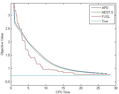
Refer to caption
Refer to caption
Refer to caption
Fig. 1: TV-based reconstruction (Shepp-Logan phantom)
Refer to caption
Refer to caption
Refer to caption
Fig. 2: TV-based reconstruction (brain image)

We make some observations about the results in Figures 1 and 2. For the first experiment, there is almost no difference between APD and NEST-S method, but FUSL outperforms both of them after 555 seconds in terms of both objective value and relative error. The second experiment clearly demonstrates the advantage of FUSL for solving CP problems with large Lipschitz constants. The Lipschitz constant of matrix A𝐴A in this instance is about 2×1082superscript1082\times 10^{8}, much larger than the Lipschitz constant (about 5.95.95.9) in the first experiment. FUSL still converges quickly and decreases the relative error to 0.050.050.05 in less than 100100100 iterations, while APD and NEST-S converge very slowly and more than 1,00010001,000 steps are required due to the large Lipschitz constants. It seems that FUSL is not so sensitive to the Lipschitz constants as the other two methods. This feature of FUSL makes it more efficient for solving large-scale CP problems which often have big Lipschitz constants.

In summary, for the TV-based image reconstruction problem (5.2), FUSL not only enjoys the completely parameter-free property (and hence no need to estimate the Lipschitz constant), but also demonstrates significant advantages for its speed of convergence and its solution quality in terms of relative error, especially for large-scale problems.

5.3 Partially parallel imaging

In this subsection, we compare the performance of the FUSL method with several related algorithms in reconstruction of magnetic resonance (MR) images from partial parallel imaging (PPI), to further confirm the observations on advantages of this method. The detailed background and description of PPI reconstruction can be found in [6]. This image reconstruction problem in two dimensional cases can be modeled as

minuCnj=1kMSjufj2+λi=1NDiu2,subscript𝑢superscript𝐶𝑛superscriptsubscript𝑗1𝑘superscriptnorm𝑀subscript𝑆𝑗𝑢subscript𝑓𝑗2𝜆superscriptsubscript𝑖1𝑁subscriptnormsubscript𝐷𝑖𝑢2\min_{u\in C^{n}}\sum_{j=1}^{k}\|M\mathcal{F}S_{j}u-f_{j}\|^{2}+\lambda\sum_{i=1}^{N}\|D_{i}u\|_{2},

where u𝑢u is the vector form of a two-dimensional image to be reconstructed, k𝑘k is the number of MR coils (consider them as sensors) in the parallel imaging system. FCn×n𝐹superscript𝐶𝑛𝑛F\in C^{n\times n} is a 2D discrete Fourier transform matrix, SjCn×nsubscript𝑆𝑗superscript𝐶𝑛𝑛S_{j}\in C^{n\times n} is the sensitivity map of the j𝑗j-th sensor, and MRn×n𝑀superscript𝑅𝑛𝑛M\in R^{n\times n} is a binary mask describes the scanning pattern. Note that the percentages of nonzero elements in M𝑀M describes the compression ration of PPI scan. In our experiments, the sensitivity map {Sj}j=1ksuperscriptsubscriptsubscript𝑆𝑗𝑗1𝑘\{S_{j}\}_{j=1}^{k} is shown in Figure 3, the image xtruesubscript𝑥𝑡𝑟𝑢𝑒x_{true} is of size 512×512512512512\times 512 shown in Figures 4 and 5, and the measurements {fj}subscript𝑓𝑗\{f_{j}\} are generated by

fj=M(FSjxtrue+ϵjre/2+ϵjim/2),j=1,,k,formulae-sequencesubscript𝑓𝑗𝑀𝐹subscript𝑆𝑗subscript𝑥𝑡𝑟𝑢𝑒subscriptsuperscriptitalic-ϵ𝑟𝑒𝑗2subscriptsuperscriptitalic-ϵ𝑖𝑚𝑗2𝑗1𝑘f_{j}=M(FS_{j}x_{true}+\epsilon^{re}_{j}/\sqrt{2}+\epsilon^{im}_{j}/\sqrt{-2}),\ j=1,\ldots,k, (5.6)

where ϵjre,ϵjimsubscriptsuperscriptitalic-ϵ𝑟𝑒𝑗subscriptsuperscriptitalic-ϵ𝑖𝑚𝑗\epsilon^{re}_{j},\epsilon^{im}_{j} are the noise with entries independently distributed according to N(0,σ)𝑁0𝜎N(0,\sigma). We conduct two experiments on this data set with different acquisition rates, and compare the FUSL method to NEST-S method, and the accelerated linearized alternating direction of multipliers (AL-ADMM) with line-search method [25].

For both experiments, set σ=3×10²,λ=105formulae-sequence𝜎3superscript102𝜆superscript105\sigma=3\times 10^{-2},\lambda=10^{-5}, and {fj}j=1ksuperscriptsubscriptsubscript𝑓𝑗𝑗1𝑘\{f_{j}\}_{j=1}^{k} are generated by (5.6). In the first experiment, we use Cartesian mask with acquisition rate 14%percent1414\%: acquire image in one row for every successive seven rows, while for the second one, we use Cartesian mask with acquisition rate 10%percent1010\%: acquire image in one row for every successive ten rows. The two masks are shown in Figure 3. The results of the first and second experiment are shown in Figures 4 and 5 respectively. These experiments again demonstrate the advantages of the FUSL method over these state-of-the-art techniques for PPI image reconstruction,

Refer to caption
Refer to caption
Refer to caption
Fig. 3: Sensitivity map and Cartesian mask
Refer to caption
Refer to caption
Refer to caption
Fig. 4: PPI image reconstruction (acquisition rate: 14%percent1414\%)
Refer to caption
Refer to caption
Refer to caption
Fig. 5: PPI image reconstruction (acquisition rate: 10%percent1010\%)

6 Concluding remarks

In this paper, we propose two new bundle-level type methods, the FAPL and FUSL methods, to uniformly solve black-box smooth, nonsmooth, and weakly smooth CP problems and a class of structured nonsmooth problems. Our methods achieve the same optimal iteration complexity and maintain all the nice features of the original APL and USL methods. Meanwhile, by simplifying the subproblems involved in the algorithms and solving them exactly, the FAPL and FUSL methods reduce the iteration cost and increase the accuracy of solutions significantly, and thus overcome the drawback of these existing bundle-level type methods applied to large-scale CP problems. Furthermore, by introducing a generic algorithmic framework, we extend the uniformly optimal bundle-level type methods to unconstrained problems and broaden the applicability of these algorithms. The complexity of bundle-level type methods for unconstrained convex optimizations has been analyzed for the first time in the literature. The numerical results for least square problems and total variation based image reconstruction clearly demonstrate the advantages of FAPL and FUSL methods over the original APL, USL and some other state-of-the-art first-order methods.

References

  • [1] Stephen Becker, Jérôme Bobin, and Emmanuel J Candès. Nesta: a fast and accurate first-order method for sparse recovery. SIAM Journal on Imaging Sciences, 4(1):1–39, 2011.
  • [2] JY Bello Cruz and W de Oliveira. Level bundle-like algorithms for convex optimization. Journal of Global Optimization, pages 1–23, 2013.
  • [3] A. Ben-Tal and A. S. Nemirovski. Non-Euclidean restricted memory level method for large-scale convex optimization. Mathematical Programming, 102:407–456, 2005.
  • [4] Ulf Brännlund, Krzysztof C Kiwiel, and Per Olof Lindberg. A descent proximal level bundle method for convex nondifferentiable optimization. Operations Research Letters, 17(3):121–126, 1995.
  • [5] Y. Chen, G. Lan, and Y. Ouyang. Optimal primal-dual methods for a class of saddle point problems. SIAM Journal on Optimization, 2014. to appear.
  • [6] Yunmei Chen, William Hager, Feng Huang, Dzung Phan, Xiaojing Ye, and Wotao Yin. Fast algorithms for image reconstruction with application to partially parallel mr imaging. SIAM Journal on Imaging Sciences, 5(1):90–118, 2012.
  • [7] W de Oliveira and CLAUDIA Sagastizábal. Level bundle methods for oracles with on-demand accuracy. Optimization Methods and Software, (ahead-of-print):1–30, 2014.
  • [8] J.E. Kelley. The cutting plane method for solving convex programs. Journal of the SIAM, 8:703–712, 1960.
  • [9] K.C. Kiwiel. Proximity control in bundle methods for convex nondifferentiable minimization. Mathematical Programming, 46:105–122, 1990.
  • [10] K.C. Kiwiel. Proximal level bundle method for convex nondifferentable optimization, saddle point problems and variational inequalities. Mathematical Programming, Series B, 69:89–109, 1995.
  • [11] KC Kiwiel. Bundle methods for convex minimization with partially inexact oracles. Comput. Optim. Appl., to appear, 2009.
  • [12] Krzysztof C Kiwiel. A proximal bundle method with approximate subgradient linearizations. SIAM Journal on optimization, 16(4):1007–1023, 2006.
  • [13] Krzysztof C Kiwiel and Claude Lemaréchal. An inexact bundle variant suited to column generation. Mathematical programming, 118(1):177–206, 2009.
  • [14] G. Lan. Bundle-level type methods uniformly optimal for smooth and non-smooth convex optimization. Manuscript, Department of Industrial and Systems Engineering, University of Florida, Gainesville, FL 32611, USA, 2013. Mathematical Programming (to appear).
  • [15] G. Lan. Bundle-type methods uniformly optimal for smooth and non-smooth convex optimization. Manuscript, Department of Industrial and Systems Engineering, University of Florida, Gainesville, FL 32611, USA, November 2010.
  • [16] C. Lemaréchal, A. S. Nemirovski, and Y. E. Nesterov. New variants of bundle methods. Mathematical Programming, 69:111–148, 1995.
  • [17] Mosek. The mosek optimization toolbox for matlab manual. version 6.0 (revision 93). http://www.mosek.com.
  • [18] A. S. Nemirovski and D. Yudin. Problem complexity and method efficiency in optimization. Wiley-Interscience Series in Discrete Mathematics. John Wiley, XV, 1983.
  • [19] Y. E. Nesterov. A method for unconstrained convex minimization problem with the rate of convergence O(1/k2)𝑂1superscript𝑘2O(1/k^{2}). Doklady AN SSSR, 269:543–547, 1983.
  • [20] Y. E. Nesterov. Introductory Lectures on Convex Optimization: a basic course. Kluwer Academic Publishers, Massachusetts, 2004.
  • [21] Y. E. Nesterov. Smooth minimization of nonsmooth functions. Mathematical Programming, 103:127–152, 2005.
  • [22] W Oliveira, C Sagastizábal, and C Lemaréchal. Bundle methods in depth: a unified analysis for inexact oracles. Optim Online Rep (Submitted), 2013.
  • [23] Welington Oliveira, Claudia Sagastizábal, and Susana Scheimberg. Inexact bundle methods for two-stage stochastic programming. SIAM Journal on Optimization, 21(2):517–544, 2011.
  • [24] Welington de Oliveira and Claudia Sagastizábal. Bundle methods in the xxist century: A bird’s-eye view. Pesquisa Operacional, 34(3):647–670, 2014.
  • [25] Yuyuan Ouyang, Yunmei Chen, Guanghui Lan, and Eduardo Pasiliao Jr. An accelerated linearized alternating direction method of multipliers. arXiv preprint arXiv:1401.6607, 2014.
  • [26] Peter Richtárik. Approximate level method for nonsmooth convex minimization. Journal of Optimization Theory and Applications, 152(2):334–350, 2012.
  • [27] Wim van Ackooij and Claudia Sagastizábal. Constrained bundle methods for upper inexact oracles with application to joint chance constrained energy problems. SIAM Journal on Optimization, 24(2):733–765, 2014.