Tight Bounds for Online Vector Scheduling

Abstract

Modern data centers face a key challenge of effectively serving user requests that arrive online. Such requests are inherently multi-dimensional and characterized by demand vectors over multiple resources such as processor cycles, storage space, and network bandwidth. Typically, different resources require different objectives to be optimized, and $L_{r}$ norms of loads are among the most popular objectives considered. Furthermore, the server clusters are also often heterogeneous making the scheduling problem more challenging.

To address these problems, we consider the online vector scheduling problem in this paper. Introduced by Chekuri and Khanna (SIAM J. of Comp. 2006), vector scheduling is a generalization of classical load balancing, where every job has a vector load instead of a scalar load. The scalar problem, introduced by Graham in 1966, and its many variants (identical and unrelated machines, makespan and $L_{r}$-norm optimization, offline and online jobs, etc.) have been extensively studied over the last 50 years. In this paper, we resolve the online complexity of the vector scheduling problem and its important generalizations — for all $L_{r}$ norms and in both the identical and unrelated machines settings. Our main results are:

• For identical machines, we show that the optimal competitive ratio is $\Theta(\log d/\log\log d)$ by giving an online lower bound and an algorithm with an asymptotically matching competitive ratio. The lower bound is technically challenging, and is obtained via an online lower bound for the minimum mono-chromatic clique problem using a novel online coloring game and randomized coding scheme. Our techniques also extend to asymptotically tight upper and lower bounds for general $L_{r}$ norms.

• For unrelated machines, we show that the optimal competitive ratio is $\Theta(\log m+\log d)$ by giving an online lower bound that matches a previously known upper bound. Unlike identical machines, however, extending these results, particularly the upper bound, to general $L_{r}$ norms requires new ideas. In particular, we use a carefully constructed potential function that balances the individual $L_{r}$ objectives with the overall (convexified) min-max objective to guide the online algorithm and track the changes in potential to bound the competitive ratio.

I Introduction

A key algorithmic challenge in modern data centers is the scheduling of online resource requests on the available hardware. Such requests are inherently multi-dimensional and simultaneously ask for multiple resources such as processor cycles, network bandwidth, and storage space [23, 34, 27] (see also multi-dimensional load balancing in virtualization [28, 32]). In addition to the multi-dimensionality of resource requests, another challenge is the heterogeneity of server clusters because of incremental hardware deployment and the use of dedicated specialized hardware for particular tasks [1, 24, 45]. As a third source of non-uniformity, the objective of the load balancing exercise is often defined by the application at hand and the resource being allocated. In addition to the traditional goals of minimizing maximum ($L_{\infty}$ norm) and total ($L_{1}$ norm) machine loads, various intermediate $L_{r}$ norms are also important for specific applications. For example, the $L_{2}$ norm of machine loads is suitable for disk storage [17, 20] while the $L_{r}$ norm for $r$ between 2 and 3 is used for modeling energy consumption [38, 3, 44].

In the algorithmic literature, the (single dimensional) load balancing problem, also called list scheduling, has a long history since the pioneering work of Graham in 1966 [26]. However, the multi-dimensional problem, introduced by Chekuri and Khanna [18] and called vector scheduling (vs), remains less understood. In the simplest version of this problem, each job has a vector load and the goal is to assign the jobs to machines so as to minimize the maximum machine load over all dimensions. As an example of our limited understanding of this problem, we note that the approximation complexity of this most basic version is not resolved yet — the current best approximation factor is $O(\log d/\log\log d)$ (e.g., [30]), where $d$ is the number of dimensions, while only an $\omega(1)$ lower bound is known [18]. In this paper, we consider the online version of this problem, i.e., where the jobs appear in a sequence and have to be assigned irrevocably to a machine on arrival. Note that this is the most common scenario in the data center applications that we described earlier, and in other real world settings. In addition to the basic setting described above, we also consider more general scenarios to capture the practical challenges that we outlined. In particular, we consider this problem in both the identical and unrelated machines settings, the latter capturing the non-uniformity of servers. Furthermore, we also consider all $L_{r}$ norm objectives of machine loads in addition to the makespan ($L_{\infty}$) objective . In this paper, we completely resolve the online complexity of all these variants of the vector scheduling problem.

Formally, there are $n$ jobs (denoted $J$) that arrive online and must be immediately and irrevocably assigned on arrival to one among a fixed set of $m$ machines (denoted $M$). We denote the $d$-dimensional load vector of job $j$ on machine $i$ by $p_{i,j}=\langle p_{i,j}(k):k\in[d]\rangle$, which is revealed on its online arrival. For identical machines, the load of job $j$ in dimension $k$ is identical for all machines $i$, and we denote it $p_{j}(k)$. Let us denote the assignment function of jobs to machines by $f:J\rightarrow M$. An assignment $f$ produces a load of $\Lambda_{i}(k)=\sum_{j:f(j)=i}p_{i,j}(k)$ in dimension $k$ of machine $i$; we succinctly denote the machine loads in dimension $k$ by an $m$-dimensional vector $\Lambda(k)$. (Note that for the scalar problem, there is only one such machine load vector.)

The makespan norm. We assume (by scaling) that the optimal makespan norm on each dimension is 1. Then, the vs problem for the makespan norm (denoted vsmax) is defined as follows.

Definition 1.

vsmax: For any dimension $k$, the objective is the maximum load over all machines, i.e.,

$$\|\Lambda(k)\|_{\infty}=\max_{i\in M}\Lambda_{i}(k).$$

An algorithm is said to be $\alpha$-competitive if $\|\Lambda(k)\|_{\infty}\leq\alpha$ for every dimension $k$. We consider this problem in both the identical machines (denoted vsmax-i) and the unrelated machines (denoted vsmax-u) settings. First, we state our result for identical machines.

Theorem 1.

There is a lower bound of $\Omega\left(\frac{\log d}{\log\log d}\right)$ on the competitive ratio of online algorithms for the vsmax-i problem. Moreover, there is an online algorithm whose competitive ratio asymptotically matches this lower bound.

The upper bound is a slight improvement over the previous best $O(\log d)$ [8, 35], but the only lower bound known previously was NP-hardness of obtaining an $O(1)$-approximation for the offline problem [18]. We remark that while the offline approximability remains unresolved, the best offline algorithms currently known ([8, 35], this paper) are in fact online. Also, our lower bound is information-theoretic, i.e., relies on the online model instead of computational limitations.

For unrelated machines (vsmax-u), an $O(\log m+\log d)$-competitive algorithm was given by Meyerson et al. [35]. We show that this is the best possible.

Theorem 2.

There is a lower bound of $\Omega(\log m+\log d)$ on the competitive ratio of online algorithms for the vsmax-u problem.

Extensions to other $L_{r}$ norms. As we briefly discussed above, there are many applications where an $L_{r}$ norm (for some $r\geq 1$) is more suitable than the makespan norm. First, we consider identical machines, and aim to simultaneously optimize all norms on all dimensions (denoted vsall-i).

Definition 2.

vsall-i: For dimension $k$ and norm $L_{r}$, $r\geq 1$, the objective is

$$\|\Lambda(k)\|_{r}=\Big{(}\sum_{i\in M}\Lambda_{i}^{r}(k)\Big{)}^{1/r}.$$

An algorithm is said to $\alpha_{r}$-competitive for the $L_{r}$ norm if $\|\Lambda(k)\|_{r}\leq\alpha_{r}$ for every dimension $k$ and every $L_{r}$ norm, $r\geq 1$. The next theorem extends Theorem 1 to an all norms optimization.

Theorem 3.

There is an online algorithm for the vsall-i problem that obtains a competitive ratio of $O\Big{(}\Big{(}\frac{\log d}{\log\log d}\Big{)}^{\frac{r-1}{r}}\Big{)}$, simultaneously for all $L_{r}$ norms. Moreover, these competitive ratios are tight, i.e., there is a matching lower bound for every individual $L_{r}$ norm.

For unrelated machines, there is a polynomial lower bound for simultaneously optimizing multiple $L_{r}$ norms, even with scalar loads. This rules out an all norms approximation. Therefore, we focus on an any norm approximation, where the algorithm is given norms $r_{1},r_{2},\ldots,r_{d}$ (where $1\leq r_{k}\leq\log m$), and the goal is to minimize the $L_{r_{k}}$ norm for dimension $k$. The same lower bound also rules out the possibility of the algorithm being competitive against the optimal value of each individual norm in their respective dimensions. We use a standard trick in multi-objective optimization to circumvent this impossibility: we only require the algorithm to be competitive against any given feasible target vector $T=\langle T_{1},\ldots,T_{d}\rangle$. For ease of notation, we assume wlog (by scaling) that $T_{k}=1$ for all dimensions $k$. Now, we are ready to define the vs problem with arbitrary $L_{r}$ norms for unrelated machines — we call this problem vsany-u.

Definition 3.

vsany-u: For dimension $k$, the objective is

$$\|\Lambda(k)\|_{r_{k}}=\Big{(}\sum_{i\in M}\Lambda_{i}^{r_{k}}(k)\Big{)}^{1/r_{k}}.$$

An algorithm is said to $\alpha_{r_{k}}$-competitive in the $L_{r_{k}}$ norm if $\|\Lambda(k)\|_{r_{k}}\leq\alpha_{r_{k}}$ for every dimension $k$. Note the (necessary) difference between the definitions of vsall-i and vsany-u: in the former, the algorithm must be competitive in all norms in all dimensions simultaneously, whereas in vsany-u, the algorithm only needs to be competitive against a single norm in each dimension that is specified in the problem input. We obtain the following result for the any norm problem.

Theorem 4.

There is an online algorithm for the vsany-u problem that simultaneously obtains a competitive ratio of $O(r_{k}+\log d)$ for each dimension $k$, where the goal is to optimize the $L_{r_{k}}$ norm in the $k$th dimension. Moreover, these competitive ratios are tight, i.e., there is a matching lower bound for every $L_{r}$ norm.

I-A Our Techniques

First, we outline the main techniques used for the identical machines setting. A natural starting point for lower bounds is the online vertex coloring (vc) lower bound of Halldórsson and Szegedy [29], for which connections to vsmax-i [18] have previously been exploited. The basic idea is to encode a vc instance as a vsmax-i instance where the number of dimensions $d$ is (roughly) $n^{B}$ and show that an approximation factor of (roughly) $B$ for vsmax-i implies an approximation factor of (roughly) $n^{1-1/B}$ for vc. One may want to try to combine this reduction and the online lower bound of $\Omega(n/\log^{2}n)$ for vc [29] to get a better lower bound for vsmax-i. However, the reduction crucially relies on the fact that a graph with the largest clique size of at most $k$ has a chromatic number of (roughly) $O(n^{1-1/k})$, and this does not imply that the graph can be colored online with a similar number of colors.

A second approach is to explore the connection of vsmax-i with online vector bin packing (vbp), where multi-dimensional items arriving online must be packed into a minimum number of identical multi-dimensional bins. Recently, Azar et al. [8] obtained strong lower bounds of $\Omega(d^{1/B})$ where $B\geq 1$ is the capacity of each bin in every dimension (the items have a maximum size of 1 on any dimension). It would be tempting to conjecture that the inability to obtain a constant approximation algorithm for the vbp  problem unless $B=\Omega(\log d)$ should yield a lower bound of $\Omega(\log d)$ for the vsmax-i problem. Unfortunately, this is false. The difference between the two problems is in the capacity of the bins/machines that the optimal solution is allowed to use: in vsmax-i, this capacity is 1 whereas in vbp, this capacity is $B$, and using bins with larger capacity can decrease the number of bins needed super-linearly in the increased capacity. Therefore, a lower bound for vbp does not imply any lower bound for vsmax-i. On the other hand, an upper bound of $O(d^{1/(B-1)}\log d)$ for the vbp problem is obtained in [8] via an $O(\log d)$-competitive algorithm for vsmax-i. Improving this ratio considerably for vsmax-i would have been a natural approach for closing the gap for vbp; unfortunately, our lower bound of $\Omega(\log d/\log\log d)$ rules out this possibility.

Our lower bound is obtained via a different approach from the ones outlined above. At a high level, we leverage the connection with coloring, but one to a problem of minimizing the size of the largest monochromatic clique given a fixed set of colors. Our main technical result is to show that this problem has a lower bound of $\Omega(\sqrt{t})$ for online algorithms, where $t$ is the number of colors. To the best of our knowledge, this problem was not studied before and we believe this result should be of independent interest. As is typical in establishing online lower bounds, the construction of the lower bound instance is viewed as a game between the online algorithm and the adversary. Our main goal is to force the online algorithm to grow cliques while guaranteeing that the optimal (offline) solution can color vertices in a way that limits clique sizes to a constant. The technical challenge is to show that the optimal solution does not form large cliques across the cliques that the algorithm has created. For this purpose, we develop a novel randomized code that dictates the choices of the optimal solution and restricts those of the online algorithm. Using the probabilistic method on this code, we are able to show the existence of codewords that always lead to a good optimal solution and an expensive algorithmic one. We also show that the same idea can be used to obtain a lower bound for any $L_{r}$ norm.

We now turn our attention to our second main result which is in the unrelated machines setting: an upper bound for the vsany-u problem. Our algorithm is greedy with respect to a potential function (as are algorithms for all special cases studied earlier [6, 4, 15, 35]), and the novelty lies in the choice of the potential function. For each individual dimension $k$, we use the $L_{r_{k}}^{r_{k}}$ norm as the potential (following [4, 15]). The main challenge is to combine these individual potentials into a single potential. We use a weighted linear combination of the individual potentials for the different dimensions. This is somewhat counter-intuitive since the combined potential can possibly allow a large potential in one dimension to be compensated by a small potential in a different one — indeed, a naïve combination only gives a competitive ratio of $O(\max_{k}r_{k}+\log d)$ for all $k$. However, we observe that we are aiming for a competitive ratio of $O(r_{k}+\log d)$ which allows some slack compared to scalar loads if $r_{k}<\log d$. Suppose $q_{k}=r_{k}+\log d$; then we use weights of $q_{k}^{-q_{k}}$ in the linear combination after changing the individual potentials to $L_{r_{k}}^{q_{k}}$. Note that as one would expect, the weights are larger for dimensions that allow a smaller slack. We show that this combined potential simultaneously leads to the asymptotically optimal competitive ratio on every individual dimension.

Finally, we briefly discuss our other results. Our slightly improved upper bound for the vsmax-i problem follows from a simple random assignment and redistributing ‘overloaded’ machines. We remark that derandomizing this strategy is relatively straightforward. Although this improvement is very marginal, we feel that this is somewhat interesting since our algorithm is simple and perhaps more intuitive yet gives the tight upper bound. For the vsall-i problem, we give a reduction to vsmax-i by structuring the instance by “smoothing” large jobs and then arguing that for structured instances, a vsmax-i algorithm is also optimal for other $L_{r}$ norms.

I-B Related Work

Due to the large volume of related work, we will only sample some relevant results in online scheduling and refer the interested reader to more detailed surveys (e.g., [7, 40, 41, 39]) and textbooks (e.g., [13]).

Scalar loads. Since the $(2-1/m)$-competitive algorithm by Graham [26] for online (scalar) load balancing on identical machines, a series of papers [10, 33, 2] have led to the current best ratio of 1.9201 [22]. On the negative side, this problem was shown to be NP-hard in the strong sense by Faigle et al. [21] and has since been shown to have a competitive ratio of at least 1.880 [11, 2, 25, 31]. For other norms, Avidor et al.[5] obtained competitive ratios of $\sqrt{4/3}$ and $2-O\left(\frac{\log r}{r}\right)$ for the $L_{2}$ and general $L_{r}$ norms respectively.

For unrelated machines, Aspnes et al. [4] obtained a competitive ratio of $O(\log m)$ for makespan minimization, which is asymptotically tight [9]. Scheduling for the $L_{2}$ norm was considered by [17, 20], and Awerbuch et al. [6] obtained a competitive ratio of $1+\sqrt{2}$, which was shown to be tight [16]. For general $L_{r}$ norms, Awerbuch et al. [6] (and Caragiannis [15]) obtained a competitive ratio of $O(r)$, and showed that it is tight up to constants. Various intermediate settings such as related machines (machines have unequal but job-independent speeds) [4, 12] and restricted assignment (each job has a machine-independent load but can only be assigned to a subset of machines) [9, 16, 19, 42] have also been studied for the makespan and $L_{r}$ norms.

Vector loads. The vsmax-i problem was introduced by Chekuri and Khanna [18], who gave an offline approximation of $O(\log^{2}d)$ and observed that a random assignment has a competitive ratio of $O\left(\frac{\log dm}{\log\log dm}\right)$. Azar et al. [8] and Meyerson et al. [35] improved the competitive ratio to $O(\log d)$ using deterministic online algorithms. An offline $\omega(1)$ lower bound was also proved in [18], and it remains open as to what the exact dependence of the approximation ratio on $d$ should be. Our online lower bound asserts that a significantly sub-logarithmic dependence would require a radically different approach from all the known algorithms for this problem.

For unrelated machines, Meyerson et al. [35] noted that the natural extension of the algorithm of Aspnes et al. [4] to vector loads has a competitive ratio of $O(\log dm)$ for makespan minimization; in fact, for identical machines, they used exactly the same algorithm but gave a tighter analysis. For the offline vsmax-u problem, Harris and Srinivasan [30] recently showed that the dependence on $m$ is not required by giving a randomized $O(\log d/\log\log d)$ approximation algorithm.

II Identical Machines

First, we consider the online vector scheduling problem for identical machines. In this section, we obtain tight upper and lower bounds for this problem, both for the makespan norm (Theorem 1) and for arbitrary $L_{r}$ norms (Theorem 3).

II-A Lower Bounds for vsmax-i and vsall-i

In this section, we will prove the lower bound in Theorem 1, i.e., show that any online algorithm for the vsmax-i problem can be forced to construct a schedule such that there exists a dimension where one machine has load $\Omega(\log d/\log\log d)$, whereas the optimal schedule has $O(1)$ load on all dimensions of all machines. This construction will also be extended to all $L_{p}$ norms (vsall-i) in order to establish the lower bound in Theorem 3.

We give our lower bound for vsmax-i in two parts. First in Section II-A1, we define a lower bound instance for an online graph coloring problem, which we call Monochromatic Clique. Next, in Section II-A2, we show how our lower bound instance for Monochromatic Clique can be encoded as an instance for vsmax-i in order to obtain the desired $\Omega(\log d/\log\log d)$ bound.

II-A1 Lower Bound for Monochromatic Clique

The Monochromatic Clique problem is defined as follows:

Monochromatic Clique: We are given a fixed set of $t$ colors. The input graph is revealed to an algorithm as an online sequence of $n$ vertices $v_{1},\ldots,v_{n}$ that arrive one at a time. When vertex $v_{j}$ arrives, we are given all edges between vertices $v_{1},v_{2},\ldots,v_{j-1}$ and vertex $v_{j}$. The algorithm must then assign $v_{j}$ one of the $t$ colors before it sees the next arrival. The objective is to minimize the size of the largest monochromatic clique in the final coloring.

The goal of the section will be to prove the following lemma, which we will use later in Section II-A2 to establish our lower bound for vsmax-i.

Theorem 5.

The competitive ratio of any online algorithm for Monochromatic Clique is $\Omega(\sqrt{t})$, where $t$ is the number of available colors.

More specifically, for any online algorithm $A$, there is an instance on which $A$ produces a monochromatic clique of size $\sqrt{t}$, whereas the optimal solution can color the graph such that the size of the largest monochromatic clique is $O(1)$.

We will frame the lower bound as a game between the adversary and the online algorithm. At a high level, the instance is designed as follows. For each new arriving vertex $v$ and color $c$, the adversary connects $v$ to every vertex in some currently existing monochromatic clique of color $c$. Since we do this for every color, this ensures that regardless of the algorithm’s coloring of $v$, some monochromatic clique grows by 1 in size (or the first vertex in a clique is introduced). Since this growth happens for every vertex, the adversary is able to quickly force the algorithm to create a monochromatic clique of size $\sqrt{t}$.

The main challenge now is to ensure that the adversary can still obtain a good offline solution. Our choice for this solution will be naïve: the adversary will simply properly color the monochromatic cliques it attempted to grow in the algorithm’s solution. Since the game stops once the algorithm has produced a monochromatic clique of size $\sqrt{t}$, and there are $t$ colors, such a proper coloring of every clique is possible. The risk with this approach is that a large monochromatic clique may now form in the adversary’s coloring from edges that cross these independently grown cliques (in other words, properly colored cliques in the algorithm’s solution could now become monochromatic cliques for the adversary). This may seem hard to avoid since each vertex is connecting to some monochromatic clique for every color. However, in our analysis we show that if on each step the adversary selects which cliques to grow in a carefully defined random fashion, then with positive probability, all properly colored cliques in the algorithm’s solution that hurt the adversary’s naïve solution are of size $O(1)$.

Instance Construction: We adopt the standard terminology used in online coloring problems (see, e.g. [29]). Namely, the algorithm will place each vertex in one of $t$ bins to define its color assignments, whereas we will use colors to refer to the color assignment in the optimal solution (controlled by the adversary). For each vertex arrival, the game is defined by the following 3-step process:

1. The adversary issues a vertex $v_{j}$ and defines $v_{j}$’s adjacencies with vertices $v_{1},\ldots,v_{j-1}$.

2. The online algorithm places $v_{j}$ in one of the available $t$ bins.

3. The adversary selects a color for the vertex.

We further divide each bin into $\sqrt{t}$ slots $1,2,\ldots,\sqrt{t}$. These slots will only be used for the adversary’s bookkeeping. Correspondingly, we partition the $t$ colors into $\sqrt{t}$ color sets $C_{1},\ldots,C_{\sqrt{t}}$, each of size $\sqrt{t}$. Each vertex will reside in a slot inside the bin chosen by the algorithm, and all vertices residing in slot $i$ across all bins will be colored by the optimal solution using a color from $C_{i}$. The high-level goal of the construction will be to produce properly colored cliques inside each slot of every bin.

Consider the arrival of vertex $v_{j}$. Inductively assume the previous vertices $v_{1},\ldots,v_{j-1}$ have been placed in the bins by the algorithm, and that every vertex within a bin lies in some slot. Further assume that all the vertices in any particular slot of a bin form a properly colored clique.

To specify the new adjacencies formed by vertex $v_{j}$ for Step 1, we will use a $t$-length $\sqrt{t}$-ary string $s_{j}$, where we connect $v_{j}$ to every vertex in slot $s_{j}[k]$ of bin $k$, for all $k=1,2,\ldots,t$. Next, for Step 2, the algorithm places $v_{j}$ in some bin $b_{j}$. We say that $v_{j}$ is then placed in slot $q_{j}=s_{j}[b_{j}]$ in bin $b_{j}$. Finally for Step 3, the adversary chooses an arbitrary color for $v_{j}$ from the colors in $C_{q_{j}}$ that have not yet been used for any vertex in slot $q_{j}$ of bin $b_{j}$. The adversary will end the instance whenever there exists a slot in some bin that contains $\sqrt{t}$ vertices. This ensures that as long as the game is running, there is always an unused color in every slot of every bin. Also observe that after this placement, the clique in slot $q_{j}$ in bin $b_{j}$ has grown in size by 1 but is still properly colored. So, this induction is well defined. This completes description of the instance (barring our choice for each adjacency string $s_{j}$). See Figures 2 and 2 for illustrations of the construction.

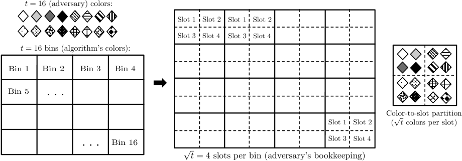
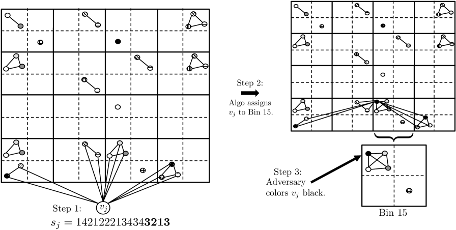
Figure 1: Illustration of the construction set-up for Lemma 5.

Figure 2: Depiction of the three-step lower-bound game for Lemma 5. For simplicity, the only adjacencies shown for vertices issued before $v_{j}$ are those between vertices in the same bin-slot pair (in reality, other adjacencies also exist). Also for simplicity, the only adjacencies shown for $v_{j}$ are those it has with vertices in bins 13 through 16 (dictated by the bold substring “3213” in $s_{j}$). Again note that in reality, $v_{j}$ will also be adjacent to vertices in bins 1 through 12 due to remaining prefix “142122213434”.

Instance Analysis: The following lemma follows directly from the construction.

Lemma 6.

For any online algorithm there is a monochromatic clique of size $\sqrt{t}$.

Proof.

After $t^{2}$ vertices are issued, there will some bin $b$ containing at least $t$ vertices, and therefore some slot in bin $b$ containing at least $\sqrt{t}$ vertices forming a clique of size $\sqrt{t}$. Since all the vertices in the clique are in the same bin, there exists a monochromatic clique of size $\sqrt{t}$ in the algorithm’s solution. ∎

Thus, it remains to show that there exists a sequence of $\sqrt{t}$-ary strings of length $t^{2}$ (recall that these strings define the adjacencies for each new vertex) such that the size of the largest monochromatic clique in the optimal coloring is $O(1)$. For brevity, we call such a sequence a good sequence.

First observe that monochromatic edges (i.e., edges between vertices of the same color) cannot form between vertices in slots $s$ and $s^{\prime}\not=s$ (in the same or in different bins) since the color sets used for the slots are disjoint. Moreover, monochromatic edges cannot form within the same slot in the same bin since these vertices always form a properly colored clique. Therefore, monochromatic edges can only form between two adjacent vertices $v_{j}$ and $v_{j^{\prime}}$ such that $q_{j}=q_{j^{\prime}}$ and $b_{j}\neq b_{j^{\prime}}$, i.e., vertices in the same slot but in different bins. Relating back to our earlier discussion, these are exactly the edges that are properly colored in the algorithm’s solution that could potentially form monochromatic cliques in the adversary’s solution; we will refer to such edges as bad edges.

Thus, in order to define a good sequence of $t^{2}$ strings, we need ensure our adjacency strings do not induce large cliques of bad edges. To do this, we first need a handle on what structure must exist across the sequence in order for bad-edge cliques to form. This undesired structure is characterized by the following lemma.

Lemma 7.

Suppose $K=\{u_{\phi(1)},\ldots,u_{\phi(w)}\}$ is a $w$-sized monochromatic clique of color $c\in C_{\ell}$ that forms during the instance, where $\phi:[w]\rightarrow[t^{2}]$ maps $k\in[w]$ to the index of the $k$th vertex to join $K$ (note, from the above discussion, that $b_{\phi(j)}$ are different for all $i\in[w]$). Then

$$s_{\phi(j)}[b_{\phi(i)}]=\ell\ \;\;\;\forall j\in\{1,\ldots,w\},\forall i\in\{1,\ldots,j-1\}.$$

Proof.

Consider vertex $u_{\phi(j)}$ (the $j$th vertex to join $K$). Since $K$ is a clique, $u_{\phi(j)}$ must be adjacent to vertices $u_{\phi(1)},\ldots,u_{\phi(j-1)}$. Since all these vertices are colored with $c\in C_{\ell}$, they must have been placed in slot $\ell$ in their respective bins. Therefore, the positions in $s_{\phi(j)}$ that correspond to these bins must also be $\ell$, i.e., $s_{\phi(j)}[b_{\phi(i)}]=\ell$ for all previous vertices $u_{\phi(i)}$. ∎

In the remainder of the proof, we show that the structure in Lemma 7 can be avoided with non-zero probability for constant sized cliques if we generate our strings uniformly at random, thus implying the existence of a good set of $t^{2}$ strings.

Specifically, suppose the adversary picks each $s_{j}$ uniformly at random, i.e., for each character in $s_{j}$ we pick $w\in[\sqrt{t}]$ with probability $t^{-1/2}$. We define the following notation:

• Let $K_{20}$ be the event that the adversary creates a monochromatic clique of size 20 or greater.

• Let $K_{20}(S,c)$ be the event that a monochromatic clique $K$ of color $c$ and size 20 or greater forms such that the first 10 vertices to join $K$ are placed in the bins specified by the set of 10 indices $S$.

• Let $P_{j}(S,q)$ be a random variable that is 1 if $s_{j}[i]=q\ \forall i\in S$ and 0 otherwise. Let $P(S,q)=\sum_{j=1}^{t^{2}}P_{j}(S,q)$.

• Let $q(c)\in[\sqrt{t}]$ to be the index of the color set to which color $c$ belongs (i.e., $c\in C_{q(c)}$).

• Let $[n]_{k}:={[n]\choose k}$ denote the set of all size-$k$ subsets of $[n]$.

The next lemma follows from standard Chernoff-Hoeffding bounds, which we state first for completeness.

Theorem 8.

(Chernoff-Hoeffding Bounds (e.g., [36])) Let $X_{1},X_{2},...,X_{n}$ be independent binary random variables and let $a_{1},a_{2},...,a_{n}$ be coefficients in $[0,1]$ . Let $X=\sum_{i}a_{i}X_{i}$. Then,

• For any $\mu\geq{\mathbb{E}}[X]$ and any $\delta>0$, $\Pr[X>(1+\delta)\mu]\leq\left(\frac{e^{\delta}}{(1+\delta)^{(1+\delta)}}\right)^{\mu}$.

• For any $\mu\leq{\mathbb{E}}[X]$ and $\delta>0$, $\Pr[X<(1-\delta)\mu]\leq e^{-\mu\delta^{2}/2}$.

We are now ready to state and prove the lemma.

Lemma 9.

If the adversary picks each $s_{j}$ uniformly at random, then $\Pr[P(S,q)\geq 10]<t^{-30}$.

Proof.

First, we observe that for any set $S\in[t]_{10}$ and any $r\in[\sqrt{t}]$, we have $\Pr[P_{i}(S,r)=1]=(1/\sqrt{t})^{10}=t^{-5}$. Therefore by linearity of expectation, we have

$${\mathbb{E}}[P(S,r)]={\mathbb{E}}\left[\sum_{i=1}^{t^{2}}P_{i}(S,r)\right]=t^{2}\cdot t^{-5}=t^{-3}.$$ (1)

Applying Theorem 8 to $P(S,r)$ with $X_{i}=P_{i}(S,r)$, $a_{i}=1$, $\delta=10t^{3}-1$ and $\mu=t^{-3}$ from Eqn. (1), we get

$$\Pr[P(S,r)\geq 10]\leq\left(\frac{e^{10t^{3}-1}}{(10t^{3})^{10t^{3}}}\right)^{t^{-3}}\leq\left(\frac{e^{10}}{10^{10}}\right)\cdot\left(\frac{1}{t^{30}}\right)<t^{-30}.\qed$$

Using Lemmas 7 and 9, we argue that there exist an offline solution with no monochromatic clique of super constant size.

Lemma 10.

There exists an offline solution where every monochromatic clique is of size $O(1)$.

Proof.

To show the existence of a good set of $t^{2}$ strings, it is sufficient to show that $\Pr[K_{20}]<1$. Using Lemma 9, we in fact show this event occurs with low probability. Observe that

$$\Pr[K_{20}]\leq\sum_{c\in[\sqrt{t}]}\sum_{S\in[t]_{10}}\Pr[K_{20}(S,c)]\leq\sum_{c\in[\sqrt{t}]}\sum_{S\in[t]_{10}}\Pr[P(S,q(c))\geq 10].$$ (2)

The first inequality is a straightforward union bound. The second inequality follows by Lemma 7. If the event $K_{20}(S,c)$ occurs, then Lemma 7 implies $s_{j}[b_{i}]=q(c)$ for $j=11,\ldots,20$, $i\in S$.

Since there are $\sqrt{t}$ possible colors and $|[t]_{10}|<t^{10}$, applying both (2) and Lemma 9 we get

$$\Pr[K_{20}]\leq\sum_{c\in[\sqrt{t}]}\sum_{S\in[t]_{10}}\Pr[P(S,q(c))\geq 10]\leq\sum_{c\in[\sqrt{t}]}\sum_{S\in[t]_{10}}t^{-30}\leq t^{1/2}\cdot t^{10}\cdot t^{-30}=t^{-39/2}<1,$$

for all $t>1$. Therefore, there is an optimal coloring such that there is no monochromatic clique of size more than 20. ∎

Theorem 5 now follows directly from Lemmas 6 and 10.

II-A2 Lower Bound for vsmax-i and vsall-i from Monochromatic Clique

We are now ready to use Theorem 5 to show an $\Omega(\log d/\log\log d)$ lower bound for vsmax-i. We will describe a lower bound instance for vsmax-i whose structure is based on an instance of monochromatic clique. This will allow us to use the lower bound instance from Theorem 5 as a black box to produce the desired lower bound for vsmax-i.

We first set the problem definition of Monochromatic clique to be for $m$ colors where $m$ is also the number of machines used in the vsmax-i instance. Let $I_{C}$ be the lower-bound instance for this problem given by Theorem 5. This produces a graph $G$ of $m^{2}$ vertices such that the algorithm forms a monochromatic clique of size $\sqrt{m}$, whereas the largest monochromatic clique in the optimal solution is of size $O(1)$. Let $G_{j}=(V_{j},E_{j})$ be the graph in $I_{C}$ after vertices $v_{1},\ldots,v_{j}$ have been issued (and so $G_{n}=G$). We define the corresponding lower bound instance for vsmax-i as follows (see Figures 3 and 4 for an illustration):

• There are $m^{2}$ jobs, which correspond to vertices $v_{1},\ldots,v_{m^{2}}$ from $I_{C}$.

• Each job has $d=\binom{m^{2}}{\sqrt{m}}$ dimensions, where each dimension corresponds to a specific $\sqrt{m}$-sized vertex subset of the $m^{2}$ vertices. Let $S_{1},\ldots,S_{d}$ be an arbitrary ordering of these subsets.

• Job vectors will be binary. Namely, the $k$th vector entry for job $j$ is 1 if $v_{j}\in S_{k}$ and the vertices in $\{v_{1},\cdots,v_{j}\}\cap S_{k}$ form a clique in $G_{j}$ (if $\{v_{1},\cdots,v_{j}\}\cap S_{k}=\{v_{j}\}$, then it is considered a 1-clique); otherwise, the $k$th entry is 0.

• Let $c_{1},\ldots,c_{m}$ define an ordering on the available colors from $I_{C}$. We match each color from $I_{C}$ to a machine in our scheduling instance. Therefore, when the vsmax-i algorithm makes an assignment for a job, we translate this machine assignment as the corresponding color assignment in $I_{C}$. Formally, if job $j$ is placed on machine $i$ in the scheduling instance, then vertex $v_{j}$ is assigned color $c_{i}$ in $I_{C}$.

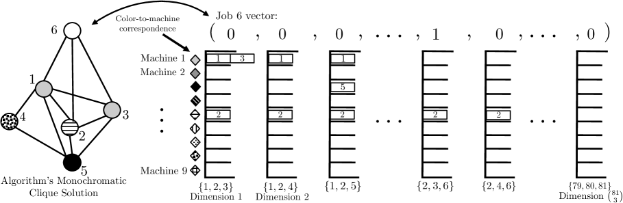
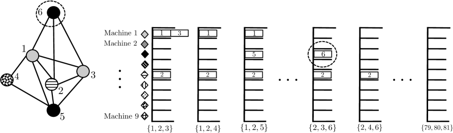
Figure 3: Illustration of the lower bound construction for vsmax-i using the monochromatic clique lower bound (Theorem 5) for an instance where $m=9$ (and thus $d={9^{2}\choose\sqrt{9}}={81\choose 3}$ for the vsmax-i instance and $t=9$ for the monochromatic clique instance). Currently job 6 is being issued; its binary load vector, which is based on the current edge structure in the monochromatic clique instance, is given above the machines/dimensions. Observe that job 6 has 0 load in the first three dimensions and the last dimension since 6 is not contained in any of the these dimensions’ $S_{k}$ sets (indicated below). It does have load 1 in the dimension corresponding to set $\{2,3,6\}$ since vertex 6 forms a clique with vertices 2 and 3 in the monochromatic clique instance; however, it still has load 0 in dimension $\{2,4,6\}$ since vertex 6 does not form a clique with vertices 2 and 4.

Figure 4: State of the construction after job 6 is assigned to machine 3. Since black is the color we associated with machine 3, this job assignment by the vsmax-i algorithm is translated as coloring vertex 6 black in the monochromatic clique instance.

Since assigning jobs to machines corresponds to colorings in $I_{C}$, it follows that the largest load in dimension $k$ is the size of the largest monochromatic sub-clique in $S_{k}$. $I_{C}$ is given by the construction in Theorem 5; therefore at the end of the instance, there will exist a dimension $k^{\prime}$ such that the online algorithm colored every vertex in $S_{k^{\prime}}$ with some color $c_{i}$. Thus, machine $i$ will have $\sqrt{m}$ load in dimension $k^{\prime}$. In contrast, Theorem 5 ensures that all the monochromatic cliques in the optimal solution are of size $O(1)$, and therefore the load on every machine in dimension $k^{\prime}$ is $O(1)$.

The relationship between $m$ and $d$ is given as follows.

Fact 11.

If $d=\binom{m^{2}}{\sqrt{m}}$, then $\sqrt{m}=\Omega(\log d/\log\log d)$.

Proof.

We will use the following well-known bounds on ${n\choose k}$: for integers $0\leq k\leq n$, $\left(\frac{n}{k}\right)^{k}\leq\binom{n}{k}\leq\left(\frac{en}{k}\right)^{k}$. First, we observe that

$$\log d=\log\binom{m^{2}}{\sqrt{m}}\leq\log\left(\frac{em^{2}}{\sqrt{m}}\right)^{\sqrt{m}}=\log(e^{\sqrt{m}}\cdot m^{(3/2)\sqrt{m}})=\sqrt{m}\cdot(1+(3/2)\log m).$$ (3)

We also have

$$\log\log d=\log\log\binom{m^{2}}{\sqrt{m}}\geq\log\log\left(\frac{m^{2}}{\sqrt{m}}\right)^{\sqrt{m}}\geq\log((3/2)\sqrt{m}\log m)\geq(1/2)\log m.$$ (4)

Hence, combining Eqns. (3) and (4), we obtain

$$\sqrt{m}\geq\frac{\log d}{1+(3/2)\log m}\geq\frac{\log d}{1+3\log\log d},$$

which implies that $\sqrt{m}=\Omega(\log d/\log\log d)$, as desired. ∎

To end the section, we show that our lower bound for vsmax-i extends to general $L_{r}$ norms (Theorem 3). As before, our lower bound construction forces any algorithm to schedule jobs so that there exists a dimension $k^{\prime}$ where at least one machine has load at least $\sqrt{m}$, whereas the load on every dimension of every machine in the optimal solution is bounded by some constant $C$. Since any dimension has at most $\sqrt{m}$ jobs with load 1, any assignment ensures that there are at most $\sqrt{m}$ machines with non-zero load in a given dimension. Therefore, in the optimal solution, the $L_{r}$-norm of the load vector for dimension $k^{\prime}$ is at most $(C^{r}\cdot\sqrt{m})^{1/r}=C\cdot m^{1/(2r)}$.

Thus, the ratio between the objective of the solution produced by the online algorithm and the optimal solution is at least $m^{1/2}/(C\cdot m^{1/2r})=(1/C)\cdot m^{(r-1)/(2r)}$. Using Fact 11, we conclude the lower bound.

II-B Upper Bounds for vsmax-i and vsall-i

In this section we prove the upper bounds in Theorem 1 (vsmax-i) and Theorem 3 (vsall-i). First, we give a randomized $O(\log d/\log\log d)$-competitive online algorithm for vsmax-i (Section II-B1) and then show how to derandomize it (Section II-B2). Next, we give an $O((\log d/\log\log d)^{\frac{r-1}{r}})$-competitive algorithm for vsall-i (Section II-B3), i.e., for each dimension $k$ and $1\leq r\leq\log m$, $\|\Lambda(k)\|_{r}$ is competitive with the optimal schedule for dimension $k$ under the $L_{r}$ norm objective.

Throughout the section we assume that a priori, the online algorithm is aware of both the final volume of all jobs on each dimension and the largest load over all dimensions and jobs. We note that the lower bounds claimed in Theorems 1 and 3 are robust against this assumption since the optimal makespan is always a constant and this knowledge does not help the online algorithm. Furthermore, these assumptions can be completely removed for our vsmax-i algorithm by updating a threshold on the maximum job load on any dimension and the total volume of jobs that the algorithm has observed so far. However, in order to make our presentation more transparent and our notation simple, we present our results under these assumptions.

For each job $j$ that arrives online, both our vsmax-i and vsall-i algorithms will perform the following transformation:

$\bullet$ Transformation 1: Let $V=\langle V_{1},\ldots,V_{d}\rangle$ be the volume vector given to the algorithm a priori, where $V_{k}$ denotes the total volume of all jobs for dimension $k$. For this transformation, we normalize $p_{j}(k)$ by dividing it by $V_{k}/m$ (for ease of notation, we will still refer to this normalized value as $p_{j}(k)$).

Our vsmax-i and vsall-i algorithms will also perform subsequent transformations; however, these transformations will differ slightly for the two algorithms.

II-B1 Randomized Algorithm for vsall-i

We now present our randomized $O(\log d/\log\log d)$-competitive algorithm for vsmax-i. Informally, our algorithm works as follows. For each job $j$, we first attempt to assign it to a machine $i$ chosen uniformly at random; however, if the resulting assignment would result in a load larger than $O(\log/\log\log d)$ on machine $i$, then we dismiss the assignment and instead assign $j$ greedily among other previously dismissed jobs. In general, a greedy assignment can be as bad as $\Omega(d)$-competitive; however, in our analysis we show that a job is dismissed by the random assignment with low probability. Therefore in expectation, the total volume of these jobs is low enough to assign greedily and still remain competitive.

Instance Transformations: Before formally defining our algorithm, we define additional online transformations and outline the properties that these transformations guarantee. Note that we perform these transformations for both the randomized algorithm presented in this section and the derandomized algorithm presented in Section II-B2. These additional transformations are defined as follows (which are preformed in sequence after Transformation 1):

• Transformation 2: Let $T$ be the load of the largest job in the instance (given a priori). If for dimension $k$ we have $T\geq V_{k}/m$, then for each job $j$ we set $p_{j}(k)$ to be $(p_{j}(k)\cdot V_{k})/(mT)$. In other words, we normalize jobs in dimension $k$ by $T$ instead of $m/V_{k}$.

• Transformation 3: For each job $j$ and dimension $k$, if $p_{j}(k)<(1/d)\max_{k^{\prime}}p_{j}(k^{\prime})$, then we increase $p_{j}(k)$ to $(1/d)\max_{k^{\prime}}p_{j}(k^{\prime})$.

Observe that after we apply Transformations 1 and 2 to all jobs, we have $\sum_{j}p_{j}(k)\leq m$ for all $k\in[d]$ and $0\leq p_{j}(k)\leq 1$ for all jobs $j$ and $k\in[d]$.

In Lemmas 12 and 13, we prove additional properties that Transformation 3 preserves. Since Transformations 1 and 2 are simple scaling procedures, an $\alpha$-competitive algorithm on the resulting scaled instance is also $\alpha$-competitive on the original instance, if we only apply the first two transformations. In Lemma 12, we prove that this property is still maintained after Transformation 3.

Lemma 12.

After Transformations 1 and 2 have been applied, Transformation 3 increases the optimal makespan by a factor of at most 2.

Proof.

Fix a machine $i$ and a dimension $k$. Let OPT denote the optimal assignment before Transformation 3 is applied. Let $J^{*}(i)$ denote the jobs assigned to machine $i$ in OPT, $\Lambda^{*}_{i}(k)$ be the load of OPT on machine $i$ in dimension $k$, and $\Lambda^{*}=\max_{i,k}\Lambda^{*}_{i}(k)$ denote the makespan of OPT. We will show that Transformation 3 can increase the load on machine $i$ in dimension $k$ by at most $\Lambda^{*}$.

Let $V_{i}^{*}=\sum_{j\in J^{*}(i)}\sum_{k^{\prime}\in[d]}p_{j}(k^{\prime})$ denote the total volume of jobs that OPT assigns to machine $i$. Observe that by a simple averaging argument, we have $V_{i}/d\leq\max_{k^{\prime}\in[d]}\Lambda^{*}_{i}(k^{\prime})$. Since Transformation 3 can increase the load of a job $j$ in a fixed dimension by at most $(1/d)\max_{k^{\prime}}p_{j}(k^{\prime})$, we can upper bound the total increase in load on machine $i$ in dimension $k$ as follows:

$$\sum_{j\in J^{*}(i)}(1/d)\max_{k^{\prime}}p_{j^{\prime}}(k^{\prime})\leq V_{i}^{*}/d\leq\ \max_{k^{\prime}\in[d]}\Lambda^{*}_{i}(k^{\prime})\leq\Lambda^{*},$$ (5)

as desired. Note that the first inequality follows from the fact that the sum of maximum loads on a machine is at most the total volume of its jobs. ∎

Recall that after Transformations 1 and 2, $\sum_{j}p_{j}(k)\leq m$ for all $k\in[d]$. In Lemma 13, we show that this property is preserved within a constant factor after Transformation 3.

Lemma 13.

After performing Transformation 3, $\sum_{j}p_{j}(k)\leq 2m$ for all $k\in[d]$.

Proof.

Consider any fixed dimension $k\in[d]$. After Transformation 3, each job $j$’s load on dimension $k$ increases by at most $(1/d)\max_{k^{\prime}}p_{j}(k^{\prime})$. Hence the total increase in load from jobs in dimension $k$ is at most

$$\sum_{j}(1/d)\max_{k^{\prime}}p_{j}(k^{\prime})\leq(1/d)\sum_{j}\sum_{k^{\prime}\in[d]}p_{j}(k^{\prime})\leq(1/d)md\leq m,$$

where the second inequality and the lemma follow from the fact that $\sum_{j}p_{j}(k)\leq m$ before Transformation 3. ∎

In summary, the properties that we collectively obtain from these transformations are as follows:

• Property 1. For all $k\in[d]$, $\sum_{j}p_{j}(k)\leq 2m$.

• Property 2. For all $j$ and $k\in[d]$, $0\leq p_{j}(k)\leq 1$.

• Property 3. For all $j$ and $k\in[d]$, $(1/d)\max_{k^{\prime}}p_{j}(k^{\prime})\leq p_{j}(k)\leq\max_{k^{\prime}}p_{j}(k^{\prime})$.

• Property 4. The optimal makespan is at least 1.

Property 1 is a restatement of Lemma 13. Property 2 was true after the first two transformations, and Transformation 3 has no effect on this property. Property 3 is a direct consequence of Transformation 3.

To see why Property 4 is true, let $j$ be the job with the largest load $T$ in the instance, and let $k=\arg\max_{k^{\prime}}p_{j}(k^{\prime})$ (i.e., $\max_{k^{\prime}}p_{j}(k^{\prime})=T$). If Transformation 2 is applied to dimension $k$, then $p_{j}(k)=1$ afterwards, which immediately implies Property 4. Otherwise, only Transformations 1 and 3 are applied to dimension $k$ and we have $\sum_{j^{\prime}}p_{j^{\prime}}(k)\geq m$, which again leads to Property 4 by a simple volume argument. Thus, by Property 4 and Lemma 12, it sufficient to show that the makespan of the algorithm’s schedule is $O(\log d/\log\log d)$.

Algorithm Definition: As discussed earlier, our algorithm consists of two procedures: a random assignment and greedy packing. It will be convenient to assume that the algorithm has two disjoint sets $M_{1}$, $M_{2}$ of $m$ identical machines that will be used independently by the two procedures, respectively. Each machine in $M_{1}$ is paired with an arbitrary distinct machine in $M_{2}$, and the actual load on a machine will be evaluated as the sum of the loads on the corresponding pair of machines. In other words, to show competitiveness it is sufficient to prove that all machines in both $M_{1}$ and $M_{2}$ have load $O(\log d/\log\log d)$.

Define the parameter $\alpha:=\frac{10\log d}{\log\log d}$. Our two procedures are formally defined as follows.

• First procedure (random assignment): Assign each job to one of the machines in $M_{1}$ uniformly at random. Let $J_{j}^{1}(i)$ denote the subset of the first $j$ jobs $\{1,2,...,j\}$ that are assigned to machine $i$ in this procedure, and let $\Lambda^{1}_{i,j}(k)$ denote the resulting load on machine $i$ on dimension $k$ due to jobs in $J_{j}^{1}(i)$. If $\Lambda^{1}_{i,j}(k)\geq 2\alpha+1$ for some $k\in[d]$, then we pass job $j$ to the second procedure. (However, note that all jobs are still scheduled by the first procedure; so even if a job $j$ is passed to the second procedure after being assigned to machine $i$ in the first procedure, $j$ still contributes load to $\Lambda_{i}^{1}(k)$ for all $k$).

• Second procedure (greedy packing): This procedure is only concerned with the jobs $J^{2}$ that are passed from the first procedure. It allocates each job in $J^{2}$ (in the order that the jobs arrive in) to one of the machines in $M_{2}$ such that the resulting makespan, $\max_{i\in M_{2},k\in[d]}\Lambda^{2}_{i,j}(k)$ is minimized; $\Lambda^{2}_{i,j}(k)$ is analogously defined for this second procedure as above.

This completes the description of the algorithm. We will let $J^{1}(i):=J^{1}_{n}(i)$ and $\Lambda^{1}_{i}(k):=\Lambda^{1}_{i,n}(k)$, and define $J^{2}(i)$ and $\Lambda^{2}_{i}(k)$ similarly. We emphasize again that jobs in $J^{2}$ are scheduled only on machines $M_{2}$; all other jobs are scheduled on $M_{1}$ machines.

Algorithm Analysis: It follows directly from the definition of the algorithm that the loads on machines in $M_{1}$ are at most $2\alpha+1=O(\log d/\log\log d)$. Therefore, we are only left with bounding the loads on machines in $M_{2}$. The following lemma shows that the second procedure receives only a small fraction of the total volume, which then allows us to argue that the greedy assignment in the second procedure is $\alpha$-competitive.

Lemma 14.

The probability that a job $j$ is passed to the second procedure is at most $1/d^{3}$, i.e. $\Pr[j\in J^{2}]\leq 1/d^{3}$.

Proof.

Fix a machine $i$, job $j$ and dimension $k$. Suppose job $j$ was assigned to machine $i$ by the first procedure and is passed to the second procedure because we would have had $\Lambda^{1}_{i,j}(k)\geq 2\alpha+1$. Since $p_{j}(k)\leq$ 1 due to Property 2, it follows that $\Lambda^{1}_{i,j-1}(k)\geq 2\alpha$. Therefore we will show

$$\Pr[\Lambda^{1}_{i,j-1}(k)\geq 2\alpha]\leq 1/d^{4},$$ (6)

where the probability space is over the random choices of jobs $1,2,...,j-1$. Once inequality (6) is established, the lemma follows from a simple union bound over all dimensions.

To show (6), we use standard Chernoff-Hoeffding bounds (stated in Theorem 8 earlier). Note that ${\mathbb{E}}[\Lambda^{1}_{i,j-1}(k)]\leq 2$ due to Property 1 and the fact that jobs are assigned to machines uniformly at random. To apply the inequality, we define random variables $X_{1},X_{2},...,X_{j-1}$ where $X_{j^{\prime}}=1$ if job $j^{\prime}$ is assigned to machine $i$; otherwise $X_{j^{\prime}}=0$. Set the parameters of Theorem 8 as follows: $a_{j^{\prime}}=p_{j^{\prime}}(k)$, $\mu=2$, and $\delta=\alpha-1$. Thus we have:

$$\Pr[\Lambda^{1}_{i,j-1}(k)\geq 2\alpha] =\Pr\left[\sum_{j^{\prime}\in[j-1]}a_{j^{\prime}}X_{j^{\prime}}\geq\alpha\mu\right]=\Pr\left[\sum_{j^{\prime}\in[j-1]}a_{j^{\prime}}X_{j^{\prime}}\geq(1+\delta)\mu\right]$$

$$\leq\left(\frac{e^{\delta}}{(1+\delta)^{(1+\delta)}}\right)^{\mu}\leq\frac{e^{\delta}}{(1+\delta)^{(1+\delta)}}$$

$$\leq 1/(5\log d/\log\log d)^{(5\log d/\log\log d)}\leq 1/d^{4}\hskip 11.38109pt\text{(for sufficiently large $d$),}$$

as desired. ∎

Next, we upper bound the makespan of the second procedure in terms of its total volume of jobs $V_{2}$, i.e. $V_{2}=\sum_{j\in J^{2},k\in[d]}p_{j}(k)$.

Lemma 15.

$\max_{i\in M_{2},k\in[d]}\Lambda^{2}_{i}(k)\leq V_{2}/m+1$.

Proof.

For sake of contradiction, suppose that at the end of the instance there exists a dimension $k$ and machine $i$ such that $\Lambda^{2}_{i}(k)>V_{2}/m+1$. Let $j$ be the job that made machine $i$ first cross this $V_{2}/m+1$ threshold in dimension $k$. For each machine $i^{\prime}$, let $k_{i^{\prime}}=\arg\max_{k^{\prime}}\Lambda_{i,j-1}^{2}(k^{\prime})$ denote the dimension with maximum load on machine $i^{\prime}$ before $j$ was assigned.

By Property 2 and the greediness of the algorithm, we have that $\Lambda_{i^{\prime},j-1}^{2}(k_{i^{\prime}})>V_{2}/m$ for all $i^{\prime}$. Otherwise, $j$ would have been assigned to a machine other than $i$ resulting in a makespan less than $V_{2}/m+1$ (since $\max_{k,j}p_{j}(k)\leq 1$). However, this implies that every machine in $M_{2}$ has a dimension with more than $V_{2}/m$ load. Clearly, this contradicts the definition of $V_{2}$. ∎

We are now ready to complete the analysis. From Lemma 14 and linearity of expectation, we know that

$${\mathbb{E}}[V_{2}]\leq\frac{1}{d^{3}}\sum_{j,k\in[d]}p_{j}(k)\leq\frac{1}{d^{3}}\cdot 2dm=\frac{m}{d^{2}},$$ (7)

where the second inequality follows from Property 1. Hence, inequality (7) along Lemma 15 imply that the second procedure yields an expected makespan of $O(1)$, which completes our analysis.

II-B2 Derandomized Algorithm for vsmax-i

Our derandomization borrows the technique developed in [14]. To derandomize the algorithm, we replace the first procedure — a uniformly random assignment — with a deterministic assignment guided by the following potential $\Phi$. Let $f(x):=\alpha^{x}$ for notational simplicity. Recall that $\alpha:=10\log d/\log\log d$.

$$\Phi_{i,k}(j) :=f\left(\Lambda^{1}_{i,j}(k)-\frac{\alpha}{m}\sum_{j^{\prime}\in[j]}p_{j^{\prime}}(k)\right) \forall i\in M_{1},j\in[n],k\in[d]$$

$$\Phi(j) :=\sum_{i\in M}\sum_{k=1}^{d}\Phi_{i,k}(j)$$

• (New deterministic) first procedure. Each job $j$ is assigned to a machine $i$ such that $\Phi(j)$ is minimized. If $\Lambda_{i,j}(k)\geq 3\alpha+1$, then $j$ is added to queue $J^{2}$ so that it can be scheduled by the second procedure. As before, each job is scheduled by either the first procedure or the second, and contributes to the “virtual” load $\Lambda_{i,j}(k)$ in either case.

Lemma 16.

$\Phi(j)$ is non-increasing in $j$.

Proof.

Consider the arrival of job $j$. To structure our argument, we assume the algorithm still assigns $j$ to a machine in $M_{1}$ uniformly at random. Our goal now is to show that ${\mathbb{E}}[\Phi(j)]\leq\Phi(j-1)$, which implies the existence of a machine $i$ such that assigning job $j$ to the machine $i$ leads to $\Phi(j)\leq\Phi(j-1)$ (and such an assignment is actually found by the algorithm since its assignment maximizes the decrease in potential). We bound ${\mathbb{E}}[\Phi_{i,k}(j)]$ as follows.

$$E[\Phi_{i,k}(j)] =\;\frac{1}{m}f\left(\Lambda_{i,j-1}+p_{j}(k)-\frac{\alpha}{m}p_{j}(k)-\frac{\alpha}{m}\sum_{j^{\prime}\in[j-1]}\Lambda_{i,j-1}(k)\right)$$

$$\;\;\;+(1-\frac{1}{m})f\left(\Lambda_{i,j-1}-\frac{\alpha}{m}p_{j}(k)-\frac{\alpha}{m}\sum_{j^{\prime}\in[j-1]}\Lambda_{i,j-1}(k)\right)$$

$$=\;\Phi_{i,k}(j-1)\cdot\alpha^{-\frac{\alpha}{m}p_{j}(k)}\cdot\left(\frac{1}{m}(\alpha^{p_{j}(k)}-1)+1\right)$$

$$\leq\;\Phi_{i,k}(j-1)\cdot\alpha^{-\frac{\alpha}{m}p_{j}(k)}\left(\frac{p_{j}(k)}{m}(\alpha-1)+1\right)$$ (8)

$$\leq\;\Phi_{i,k}(j-1)\cdot\exp\left(-(\alpha\log\alpha)\cdot\frac{p_{j}(k)}{m}\right)\exp\left(\frac{p_{j}(k)}{m}\cdot(\alpha-1)\right)$$ (9)

$$\leq\;\Phi_{i,k}(j-1)$$

Inequality (8) follows since $\alpha^{x}-1\leq(\alpha-1)x$ for $x\in[0,1]$, and $p_{j}(k)\leq 1$ due to Property 2. Inequality (9) follows from the fact that $x+1\leq e^{x}$. Therefore, by linearity of expectation, we have ${\mathbb{E}}[\Phi(j)]\leq\Phi(j-1)$, thereby proving the lemma. ∎

The next corollary follows from Lemma 16 and the simple observation that $\Phi(0)=md$.

Corollary 17.

$\Phi(n)\leq md$.

As in Section II-B1, it is straightforward to see that the algorithm forces machines in $M_{1}$ to have makespan $O(\alpha)$, so we again focus on the second procedure of the algorithm. Here, we need a deterministic bound on the total volume $V_{2}=\sum_{j\in J^{2}}\sum_{k\in[d]}p_{j}(k)$ that can be scheduled on machines in $M_{2}$. Lemma 18 provides us with such a bound.

Lemma 18.

$V_{2}\leq m/d$.

Proof.

Consider a job $j\in J_{2}$ that was assigned to machine $i$ in the first procedure. Let $k(j)$ be an arbitrary dimension $k$ with $\Lambda^{1}_{i,j}\geq 3\alpha+1$ (such a dimension exists since $j\in J^{2}$). Let $J^{2}_{i}(k)=\{j:j\in J^{1}(i)\cap J^{2}\text{ and }k(j)=k\}$ denote the set of jobs $j\in J^{2}$ that were assigned to machine $i$ by the first procedure and are associated with dimension $k$. We upper bound $V_{2}$ as follows:

$$V_{2} =\;\sum_{j\in J^{2}}\sum_{k^{\prime}\in[d]}p_{j}(k^{\prime})$$

$$=\;\sum_{i\in M_{1},k\in[d]}\sum_{j\in J^{2}_{i}(k)}\sum_{k^{\prime}\in[d]}p_{j}(k^{\prime}) j\in J^{2} k(j)$$ (since we associate job with a unique dimemsion  )

$$\leq\;\sum_{i\in M_{1},k\in[d]}\sum_{j\in J^{2}_{i}(k)}d^{2}p_{j}(k)$$ (by Property 3)

$$\leq\;d^{2}\sum_{i\in M_{1}}\sum_{k\in[d]}(\Lambda^{1}_{i}(k)-3\alpha)_{+}$$ (10)

To see why the last inequality holds, recall that $\Lambda^{1}_{i,j}(k)\geq 3\alpha+1$ when $j\in J^{1}(i)$ and $k=k(j)$. This can happen only when $\Lambda^{1}_{i,j-1}(k)\geq 3\alpha$ since $p_{j}(k)\leq 1$ due to Property 2. Since $\Lambda^{1}_{i,j^{\prime}}(k)$ is non-decreasing in $j^{\prime}$, the sum of $p_{j}(k)$ over all such jobs $j$ is at most $(\Lambda^{1}_{i}(k)-3\alpha)_{+}$; here $(x)_{+}:=\max\{0,x\}$.

We claim that for all $i\in M_{1},k\in[d]$,

$$\Phi_{i,k}(n)\geq\alpha^{\alpha}(\Lambda^{1}_{i,j}(k)-3\alpha)_{+}$$ (11)

If $\Lambda^{1}_{i,j}(k)-3\alpha\leq 0$, then the claim is obviosuly true since $\Phi_{i,k}(n)$ is always non-negative. Otherwise, we have

$$\Phi_{i,k}(n)\geq\alpha^{\Lambda^{1}_{i,n}(k)-2\alpha}\geq\alpha^{\alpha}(\Lambda_{i,j}(k)-3\alpha),$$

where the first inequlaity follows from Property 1. So in either case, (11) holds.

By combining (10), (11), Corollary 17, and recalling $\alpha=\frac{10\log d}{\log\log d}$, we have

$$V_{2}\leq d^{2}\sum_{i}\sum_{k}(\Lambda^{1}_{i}(k)-3\alpha)_{+}\leq\frac{d^{2}}{\alpha^{\alpha}}\sum_{i}\sum_{k}\Phi_{i,k}(n)\leq\frac{d^{3}}{\alpha^{\alpha}}m\leq\frac{m}{d}.\qed$$

By Lemma 15, we have $\max_{i\in M_{2},k\in[d]}\Lambda^{2}_{i}(k)\leq\frac{1}{m}V_{2}+1=O(1)$. Thus, we have shown that each of the two deterministic procedures yields a makespan of $O(\alpha)=O(\log d/\log\log d)$, thereby proving the upper bound.

II-B3 Algorithm for vsall-i

We now give our $O((\log d/\log\log d)^{\frac{r-1}{r}})$-competitive algorithm for vsall-i. Throughout the section, let $A$ denote the $O(\log d/\log\log d)$-competitive algorithm for vsmax-i defined in Section II-B2. Our vsall-i algorithm essentially works by using $A$ as a black box; however, we will perform a smoothing transformation on large loads before scheduling jobs with $A$.

Algorithm Definition: We will apply the following transformation to all jobs $j$ that arrive online after Transformation 1 has been performed (note that this is in replacement of Transformations 2 and 3 defined in Section II-B1).

$\bullet$ Transformation 2: If $p_{j}(k)>1$, we reduce $p_{j}(k)$ to be 1. If this load reduction is applied in dimension $k$ for job $j$, we say $j$ is large in $k$; otherwise, $j$ is small in dimension $k$.

It is straightforward to see that Transformations 1 and 2 provide the following two properties:

• Property 1: $\sum_{j\in J}p_{j}(k)\leq m$ for all $k\in[d]$.

• Property 2: $0\leq p_{j}(k)\leq 1$ for all $j\in J,k\in[d]$.

On this transformed instance, our algorithm simply schedules jobs using our vsmax-i algorithm $A$.

Algorithm Analysis: Let $\alpha=O(\log d/\log\log d$) be the competitive ratio of algorithm $A$. Clearly if we can establish $\alpha^{(r-1)/r}$-competitiveness for the scaled instance (i.e. just applying Transformation 1 to all jobs but not Transformation 2), then our algorithm is competitive on the original instance as well. Let OPT${}^{\prime}(k,r)$ be the cost of the optimal solution on the scaled loads in dimension $k$. In Lemma 19, we establish two lower bounds on OPT${}^{\prime}(k,r)^{r}$.

Lemma 19.

$\displaystyle\text{{\sc OPT}}^{\prime}(k,r)^{r}\geq\max\left(\sum_{j\in J}p_{j}(k)^{r},m\cdot\left(\sum_{j\in J}p_{j}(k)/m\right)^{r}\right)=\max\left(\sum_{j\in J}\left(p_{j}(k)^{r}\right),m\right).$

Proof.

Consider any fixed assignment of jobs, and let $J^{\prime}(i)\subseteq J$ be the set of jobs assigned to machine $i$. Consider any fixed $k$. The first lower bound (within the max in the statement of the lemma) follows since

$$\sum_{i\in M}\left(\sum_{j\in J^{\prime}(i)}p_{j}(k)\right)^{r}\geq\sum_{i\in M}\sum_{j\in J^{\prime}(i)}p_{j}(k)^{r}=\sum_{j\in J}p_{j}(k)^{r}.$$

The second lower bound is due to the convexity of $x^{r}$ when $r\geq 1$. ∎

Let $J(i)\subseteq J$ be the set of jobs assigned to machine $i$ by the online algorithm. Let $\ell(i,k)$ and $s(i,k)$ be the set of jobs assigned to machine $i$ that are large and small in dimension $k$, respectively. For brevity, let $\sigma_{\ell}(i,k)=\sum_{j\in\ell(i,k)}p_{j}(k)$ and $\sigma_{s}(i,k)=\sum_{j\in s(i,k)}p_{j}(k)$. Observe that since algorithm $A$ is $\alpha$-competitive on an instance with both Properties 1 and 2, we obtain the following additional two properties for the algorithm’s schedule:

• Property 3: $|\ell(i,k)|\leq\alpha$ for all $i\in M,k\in[d]$.

• Property 4: $\sigma_{s}(i,k)\leq\alpha$ for all $i\in M,k\in[d]$.

Using these additional properties, the next two lemmas will bound the contribution of both large and small loads to the objective; namely, we need to bound both $\sigma_{\ell}(i,k)^{r}$ and $\sum_{i}\sigma_{s}(i,k)^{r}$ in terms of $\alpha$. Lemma 20 provides this bound for large loads, while Lemma 21 will be used to bound small loads.

Lemma 20.

$\sigma_{\ell}(i,k)^{r}=\left(\sum_{j\in\ell(i,k)}p_{j}(k)\right)^{r}\leq\alpha^{r-1}\sum_{j\in\ell(i,k)}p_{j}(k)^{r}.$

Proof.

Let $h=|\ell(i,k)|$. Then, it follows that

$$\left(\sum_{j\in\ell(i,k)}p_{j}(k)\right)^{r} =\left(\frac{1}{h}\sum_{j\in\ell(i,k)}(p_{j}(k)\cdot h)\right)^{r}\leq\frac{1}{h}\sum_{j\in\ell(i,k)}(p_{j}(k)\cdot h)^{r} x^{r}$$ (due to the convexity of )

$$=h^{r-1}\sum_{j\in\ell(i,k)}p_{j}(k)^{r}\leq\alpha^{r-1}\sum_{j\in\ell(i,k)}p_{j}(k)^{r} \hskip 14.22636pt\text{(by Property 3)}.\qed$$

Recall that by Property 1, we have that $\sigma_{s}(i,k)\leq m$. Using this fact and along with Property 4, the general statement shown in Lemma 21 will immediately provide us with the desired bound on $\sum_{i}\sigma_{s}(i,k)^{r}$ (stated formally in Corollary 22).

Lemma 21.

Let $f(x)=x^{r}$ for some $r\geq 1$ whose domain is defined over a set of variables $x_{1},\ldots,x_{n}\in[0,\alpha]$ where $\alpha\geq 1$. If $\sum_{i=1}^{m}x_{i}\leq m$, then

$$\sum_{i=1}^{m}f(x_{i})\leq 2m\ \alpha^{r-1}.$$

Proof.

Let $\tilde{f}=\sum_{i=1}^{m}f(x_{i})$. We claim that $\tilde{f}$ is maximized when $0<x_{i}<\alpha$ for at most one $i\in[m]$. If there are two such variables $x_{i}$ and $x_{j}$ with $0<x_{i}\leq x_{j}<\alpha$, it is easy to see that we can further increase $\tilde{f}$ by decreasing $x_{i}$ and increasing $x_{j}$ by an infinitesimal equal amount (i.e. $x_{i}\leftarrow x_{i}-\epsilon$ and $x_{j}\leftarrow x_{j}+\epsilon$) due to convexity of $f$.

Hence, the $\tilde{f}$ is maximized when the multi-set $\{x_{i}:i\in[m]\}$ has $\lfloor m/\alpha\rfloor$ copies of $\alpha$, and one copy of $m-\alpha\lfloor m/\alpha\rfloor$ (which is at most $\alpha$), which gives,

$$\tilde{f}\leq\lfloor m/\alpha\rfloor f(\alpha)+f(m-\alpha\lfloor m/\alpha\rfloor).$$ (12)

If $\lfloor m/\alpha\rfloor\geq 1$, then it follows that

$$\sum_{i=1}^{m}f(x_{i})=\tilde{f} \leq(\lfloor m/\alpha\rfloor+1)f(\alpha) m-\alpha\lfloor m/\alpha\rfloor\leq\alpha)$$ (by Eqn. (12) and since

$$\leq 2(m/\alpha)\alpha^{r}=2m\ \alpha^{r-1} \lfloor m/\alpha\rfloor\geq 1$$ (since ).

In the case where $m<\alpha$, $\tilde{f}$ is maximized by making single $x_{i}=m$. Therefore $\tilde{f}\leq f(m)=m^{r}\leq m\alpha^{r-1}$. ∎

Corollary 22.

For all dimensions $k$, $\sum_{i\in M}\sigma_{s}(i,k)^{r}\leq 2m\ \alpha^{r-1}$.

We are now ready to bound $\|\Lambda(k)\|_{r}$ against $\text{{\sc OPT}}^{\prime}(k,r)$.

Lemma 23.

For all dimensions $k$, $\|\Lambda(k)\|_{r}=O(\alpha^{(r-1)/r})\text{{\sc OPT}}^{\prime}(k,r)$, i.e., the $L_{r}$ norm of the vector load is at most $O(\alpha^{(r-1)/r})$ times the $L_{r}$ norm of the vector load of the optimal solution.

Proof.

Using Lemmas 19, 20, and Corollary 22, we have the following bound for $|\Lambda(k)\|_{r}^{r}=\sum_{i\in M}\left(\sum_{j\in J(i)}p_{j}(k)\right)^{r}$:

$$\sum_{i\in M}\left(\sum_{j\in J(i)}p_{j}(k)\right)^{r} =\sum_{i\in M}\left(\sum_{j\in\ell(i,k)}p_{j}(k)+\sum_{j\in s(i,k)}p_{j}(k)\right)^{r}$$

$$\leq\sum_{i\in M}\left(2\max\left(\sum_{j\in\ell(i,k)}p_{j}(k),\sum_{j\in s(i,k)}p_{j}(k)\right)\right)^{r}$$

$$\leq 2^{r}\sum_{i\in M}\left(\left(\sum_{j\in\ell(i,k)}p_{j}(k)\right)^{r}+\left(\sum_{j\in s(i,k)}p_{j}(k)\right)^{r}\right)$$

$$\leq 2^{r}\left(\alpha^{r-1}\sum_{j\in\ell(i,k)}p_{j}(k)^{r}+2m\cdot\alpha^{r-1}\right)$$ (by Lemma 20 and Corollary 22)

$$\leq(2^{r+1}\alpha^{r-1})\text{{\sc OPT}}^{\prime}(k,r)^{r}$$ (by Lemma 19)

which, raising both the LHS and RHS to $1/r$, gives us

$$\|\Lambda(k)\|_{r}\leq\left(2^{1+1/r}\alpha^{(r-1)/r}\right)\text{{\sc OPT}}^{\prime}(k,r)=O(\alpha^{(r-1)/r})\text{{\sc OPT}}^{\prime}(k,r).$$

∎

The upper bound in Theorem 3 now follows immediately from Lemma 23.

III Unrelated Machines

Now, we consider the online vector scheduling problem for unrelated machines. In this section, we obtain tight upper and lower bounds for this problem, both for the makespan norm (Theorem 2) and for arbitrary $L_{r}$ norms (Theorem 4).

III-A Lower Bound for vsany-u

In this section we prove the lower bound in Theorem 4, i.e., we show that we can force any algorithm to make an assignment where there exists a dimension $k$ that has cost at least $\Omega(\log d+r_{k})$ where $1\leq r_{k}\leq\log m$.

Our construction is an adaptation of the lower bounds in [15] and [6] but for a multidimensional setting. Informally, the instance is defined as follows. We set $m=d$ and then associate $i$th machine with the $i$th dimension, i.e., machine $i$ only receives load in the $i$th dimension. We then issue jobs in a series of $\log d+1$ phases. In a given phase, there will be a current set of active machines, which are the only machines that can be loaded in the current phase and for the rest of the instance (so once a machine is inactivated it stays inactive). More specifically, in a given phase we arbitrarily pair off the active machines and then issue one job for each pair, where each job has unit load but is defined such that it must be assigned to a unique machine in its pair. When a phase completes, we inactivate all the machines that did not receive load (so we cut the number of active machines in half). This process eventually produces a load of $\log d+1$ on some machine, whereas reversing the decisions of the algorithm gives an optimal schedule where $L_{k}=1$ for all $k\in[d]$.

More formally let $d=2^{h}$. The adversary sets the instance target parameters to be $T_{k}=1$ for all $k\in[d]$ (it will be clear from our construction that these targets are feasible). For each job $j$, let $m_{1}(j),m_{2}(j)\in[m]$ denote the machine pair the adversary associates with job $j$. We define $j$ to have unit load on machines $m_{1}(j)$, $m_{2}(j)$ in their respective dimensions and arbitrarily large load on all other machines. Formally, $p_{i,j}(k)$ is defined to be

$$p_{i,j}(k)=\left\{\begin{array}[]{ll}0&\text{if $i\neq k$ and $i\in\{m_{1}(j),m_{2}(j)\}$}\\ 1&\text{if $i=k$ and $i\in\{m_{1}(j),m_{2}(j)\}$}\\ \infty&\text{otherwise}.\end{array}\right.$$

As discussed above, the adversary issues jobs in $h+1$ phases. Phases $1$ through $h$ will work as previously specified (we describe how the final $(h+1)$th phase works shortly). Let $S_{\ell}$ denote the active machines in phase $\ell$. In the $\ell$th phase, we issue a set of jobs $J_{\ell}$ where $|J_{\ell}|=2^{h-\ell}$. We then pair off the machines in $S_{\ell}$ and use each machine pair as $m_{1}(j)$ and $m_{2}(j)$ for a unique job $j\in J_{\ell}$. Clearly the algorithm must schedule $j$ on $m_{1}(j)$ or $m_{2}(j)$, and thus $2^{h-\ell}$ machines accumulate an additional load of 1 in phase $\ell$. Machines that receive jobs in phase $\ell$ remain active in phase $\ell+1$; all other machines are set to be inactive. In the final phase $h+1$, there will be a single remaining active machine $i^{\prime}$; thus, we issue a single job $j^{\prime}$ with unit load that must be scheduled on $i^{\prime}$ (note that this final phase is added to the instance only to make our target vector feasible).

Based on this construction, there will exist a dimension $k^{\prime}$ at the end of the instance that has load $h+1$ on machine $k^{\prime}$ and 0 on all other machines. Observe that the optimal schedule is obtained by reversing the decisions of the algorithm, which places a unit load on one machine in each dimension. Namely, if $j$ was assigned to $m_{1}(j)$, then the optimal schedule assigns $j$ to $m_{2}(j)$ (and vice versa), with the exception that $j^{\prime}$ is assigned to its only feasible machine.

In the case that $\log d\geq r_{k^{\prime}}$, the adversary stops. Since $T_{k^{\prime}}=1$ and $L_{k^{\prime}}=h+1=\log d+1$, we have that $L_{k^{\prime}}/T_{k^{\prime}}=\Omega(\log d+r_{k})$. If $\log d<r_{k^{\prime}}$, then the adversary stops the current instance and begins a new instance. In the new instance, we simply simulate the lower bound from [6] in dimension $k^{\prime}$ (i.e., the only dimension that receives load is dimension $k^{\prime}$; the adversary also resets the target vectors accordingly). Here, the adversary forces the algorithm to be $\Omega(r_{k^{\prime}})$-competitive, which, since $\log d<r_{k^{\prime}}$, gives us the desired bound of $\Omega(\log d+r_{k^{\prime}})$.

III-B Upper Bound

Our goal is to prove the upper bound in Theorem 4. Recall that we are given targets $T_{k}$, and we have to show that $\|\Lambda(k)\|_{r_{k}}=O(\log d+r_{k})\cdot T_{k}$ for all $k\in[d]$. ($\Lambda(k)$ is the load vector in dimension $k$ and $r_{k}$ is the norm that we are optimizing.) First, we normalize $p_{i,j}(k)$ to $p_{i,j}(k)/T_{k}$ for all dimensions $k$; to keep the notation simple, we will also denote this normalized load $p_{i,j}(k)$. This ensures that the target objective is 1 in every dimension. (We assume wlog that $T_{k}>0$. If $T_{k}=0$, the algorithm discards all assignments that put non-zero load on dimension $k$).

III-B1 Description of the Algorithm

As described in the introduction, our algorithm is greedy with respect to a potential function defined on modified $L_{r_{k}}$ norms. Let $L_{k}=\|\Lambda(k)\|_{r_{k}}$ denote the $L_{r_{k}}$-norm of the machine loads in the $k$th dimension, and $q_{k}=r_{k}+\log d$ denote the desired competitive ratio; all logs are base 2. We define the potential for dimension $k$ as $\Phi_{k}=L_{k}^{q_{k}}$. The potentials for the $d$ different dimensions are combined using a weighted linear combination, where the weight of dimension $k$ is $\alpha_{k}=(3q_{k})^{-q_{k}}$. Note that dimensions that allow a smaller slack in the competitive ratio are given a larger weight in the potential. We denote the combined potential by $\Phi=\sum_{k=1}^{d}\alpha_{k}\cdot\Phi_{k}$. The algorithm assigns job $j$ to the machine that minimizes the increase in potential $\Phi$.

III-B2 Competitive analysis

Let us fix a solution satisfying the target objectives, and call it the optimal solution. Let $\Lambda_{i}(k)$ and $\Lambda_{i}^{*}(k)$ be the load on the $i$th machine in the $k$th dimension for the algorithmic solution and the optimal solution respectively. We also use $L^{*}_{k}$ to denote the $L_{r_{k}}$ norm in the $k$th dimension for the optimal solution; we have already asserted that by scaling, $L^{*}_{k}=1$.

Similar to [4, 15], we compare the actual assignment made by the algorithm (starting with zero load on every machine in every dimension) to a hypothetical assignment made by the optimal solution starting with the final algorithmic load on every machine (i.e., load of $\Lambda_{i}(k)$ on machine $i$ in dimension $k$).

We will need the following fact for our analysis, which follows by observing that all parameters are positive, the function is continuous in the domain, and its derivative is non-negative.

Fact 24.

The function $f(x_{1},x_{2},$ $\ldots,x_{m})=\left(\sum_{i}(x_{i}+a_{i})^{w}\right)^{z}-\left(\sum_{i}x_{i}^{w}\right)^{z}$ is non-decreasing if for all $i\in[m]$ we restrict the domain of $x_{i}$ to be $[0,\infty)$, $w\geq 1,z\geq 1$, and $a_{i}\geq 0$.

Using greediness of the algorithm and convexity of the potential function, we argue in Lemma 25 that the change in potential in the former process is upper bounded by that in the latter process.

Lemma 25.

The total change in potential in the online algorithm satisfies:

$$\sum_{k=1}^{d}\alpha_{k}L_{k}^{q_{k}}=\Phi(n)-\Phi(0)\leq\sum_{k=1}^{d}\alpha_{k}\Big{(}\sum_{i=1}^{m}\Big{(}\Lambda_{i}(k)+\Lambda_{i}^{*}(k)\Big{)}^{r_{k}}\Big{)}^{q_{k}/r_{k}}-\sum_{k=1}^{d}\alpha_{k}L_{k}^{q_{k}}$$

Proof.

Let $y_{i,j}=1$ if the algorithm assigns job $j$ to machine $i$; otherwise, $y_{i,j}=0$. Define $y_{i,j}^{*}$ similarly but for the optimal solution’s assignments. We can express the resulting change in potential from scheduling job $j$ as follows.

$$\Phi(j)-\Phi(j-1) =\sum_{k=1}^{d}\alpha_{k}\left(L_{k}^{q_{k}}(j)-L_{k}^{q_{k}}(j-1)\right)=\sum_{k=1}^{d}\alpha_{k}\Big{(}\Big{(}\sum_{i=1}^{m}\Lambda_{i,j}^{r_{k}}(k)\Big{)}^{q_{k}/r_{k}}-\Big{(}\sum_{i=1}^{m}\Lambda_{i,j-1}^{r_{k}}(k)\Big{)}^{q_{k}/r_{k}}\Big{)}$$ (13)

$$=\sum_{k=1}^{d}\alpha_{k}\Big{(}\Big{(}\sum_{i=1}^{m}\Big{(}\Lambda_{i,j-1}(k)+p_{i,j}(k)\cdot y_{i,j}\Big{)}^{r_{k}}\Big{)}^{q_{k}/r_{k}}-\Big{(}\sum_{i=1}^{m}\Lambda_{i,j-1}^{r_{k}}(k)\Big{)}^{q_{k}/r_{k}}\Big{)}.\vspace{-2mm}$$

Since the online algorithm schedules greedily based on $\Phi(j)$, using optimal schedule’s assignment for job $j$ must result in a potential increase that is at least as large. Therefore by (13) we have

$$\Phi(j)-\Phi(j-1)\leq\sum_{k=1}^{d}\alpha_{k}\Big{(}\Big{(}\sum_{i=1}^{m}\Big{(}\Lambda_{i,j-1}(k)+p_{i,j}(k)\cdot y^{*}_{i,j}\Big{)}^{r_{k}}\Big{)}^{q_{k}/r_{k}}-\Big{(}\sum_{i=1}^{m}\Lambda_{i,j-1}^{r_{k}}(k)\Big{)}^{q_{k}/r_{k}}\Big{)}.\\$$ (14)

As loads are non-decreasing, $\Lambda_{i}(k)\geq\Lambda_{i,j-1}(k)$. Also note that $r_{k}\geq 1$ and

$$q_{k}/r_{k}=(r_{k}+\log d)/r_{k}>1.$$

Thus, we can apply Fact 24 to (14) (setting $w=r_{k}$, $z=q_{k}/r_{k}$, and $a_{i}=p_{i,j}(k)\cdot y^{*}_{i,j}$) to obtain

$$\Phi(j)-\Phi(j-1)\leq\sum_{k=1}^{d}\alpha_{k}\Big{(}\Big{(}\sum_{i=1}^{m}\Big{(}\Lambda_{i}(k)+p_{i,j}(k)\cdot y^{*}_{i,j}\Big{)}^{r_{k}}\Big{)}^{q_{k}/r_{k}}-\Big{(}\sum_{i=1}^{m}\Lambda_{i}^{r_{k}}(k)\Big{)}^{q_{k}/r_{k}}\Big{)}.\\$$ (15)

We can again use Fact 24 to further bound the potential increase (using the same values of $a_{i}$, $w$, and $z$, but now $x_{i}=\Lambda_{i,j-1}^{*}(k)$):

$$\Phi(j)-\Phi(j-1) \leq\sum_{k=1}^{d}\alpha_{k}\Big{(}\Big{(}\sum_{i=1}^{m}\Big{(}\Lambda_{i}(k)+\Lambda^{*}_{i,j-1}(k)+p_{i,j}(k)\cdot y^{*}_{ij}\Big{)}^{r_{k}}\Big{)}^{q_{k}/r_{k}}-\Big{(}\sum_{i=1}^{m}\Big{(}\Lambda_{i}(k)+\Lambda_{i,j-1}^{*}(k)\Big{)}^{r_{k}}\Big{)}^{q_{k}/r_{k}}\Big{)}$$

$$=\sum_{k=1}^{d}\alpha_{k}\Big{(}\Big{(}\sum_{i=1}^{m}\Big{(}\Lambda_{i}(k)+\Lambda_{i,j}^{*}(k)\Big{)}^{r_{k}}\Big{)}^{q_{k}/r_{k}}-\Big{(}\sum_{i=1}^{m}\Big{(}\Lambda_{i}(k)+\Lambda_{i,j-1}^{*}(k)\Big{)}^{r_{k}}\Big{)}^{q_{k}/r_{k}}\Big{)}.$$ (16)

Observe that for a fixed $k$, the RHS of (16) is a telescoping series if we sum over all jobs $j$:

$$\sum_{j=1}^{n}\alpha_{k}\Big{(}\Big{(}\sum_{i=1}^{m}\Big{(}\Lambda_{i}(k)+\Lambda_{i,j}^{*}(k)\Big{)}^{r_{k}}\Big{)}^{q_{k}/r_{k}}-\Big{(}\sum_{i=1}^{m}\Big{(}\Lambda_{i}(k)+\Lambda_{i,j-1}^{*}(k)\Big{)}^{r_{k}}\Big{)}^{q_{k}/r_{k}}\Big{)}$$

$$= \alpha_{k}\Big{(}\sum_{i=1}^{m}\Big{(}\Lambda_{i}(k)+\Lambda_{i}^{*}(k)\Big{)}^{r_{k}}\Big{)}^{q_{k}/r_{k}}-\Big{(}\sum_{i=1}^{m}\Big{(}\Lambda_{i}(k)\Big{)}^{r_{k}}\Big{)}^{q_{k}/r_{k}}.$$

We have

$$\sum_{j=1}^{n}(\Phi(j)-\Phi(j-1))=\Phi(n)-\Phi(0),$$

since this is also a telescoping series. By definition, $\Phi(0)=0$ and $\Phi(n)=\sum_{k=1}^{d}\alpha_{k}L_{k}^{q_{k}}$. Using these facts along with (16) and (III-B2), we establish the lemma:

$$\sum_{k=1}^{d}\alpha_{k}L_{k}^{q_{k}} = \sum_{j=1}^{n}(\Phi(j)-\Phi(j-1))\hskip 14.22636pt\text{(since $\Phi$ telescopes, $\Phi(0)=0$, and $\Phi(n)=\sum_{k=1}^{d}\alpha_{k}L_{k}^{q_{k}}$)}$$

$$\leq \sum_{k=1}^{d}\alpha_{k}\Big{(}\sum_{i=1}^{m}\Big{(}\Lambda_{i}(k)+\Lambda_{i}^{*}(k)\Big{)}^{r_{k}}\Big{)}^{q_{k}/r_{k}}-\sum_{k=1}^{d}\alpha_{k}L_{k}^{q_{k}}\Big{)}\hskip 14.22636pt\text{(by \eqref{eq:pot3} and \eqref{eq:pot4})}.\qed$$

We proceed by applying Minkowski inequality (e.g., [43]), which states that for any two vectors $v_{1}$ and $v_{2}$, we have $\|v_{1}+v_{2}\|_{r}\leq\|v_{1}\|_{r}+\|v_{2}\|_{r}$. Applying this inequality to the RHS in Lemma 25, we obtain

$$\sum_{k=1}^{d}\alpha_{k}L_{k}^{q_{k}} \leq\sum_{k=1}^{d}\alpha_{k}\Big{(}\Big{(}\sum_{i=1}^{m}\Lambda_{i}^{r_{k}}(k)\Big{)}^{1/r_{k}}+\Big{(}\sum_{i=1}^{m}(\Lambda_{i}^{*}(k))^{r_{k}}\Big{)}^{1/r_{k}}\Big{)}^{q_{k}}-\sum_{k=1}^{d}\alpha_{k}L_{k}^{q_{k}}$$

$$=\sum_{k=1}^{d}\alpha_{k}\Big{(}L_{k}+L_{k}^{*}\Big{)}^{q_{k}}-\sum_{k=1}^{d}\alpha_{k}L_{k}^{q_{k}}.$$ (17)

Next, we prove a simple lemma that we will apply to inequality (17).

Lemma 26.

$(L_{k}+L_{k}^{*})^{q_{k}}\leq e^{1/2}L_{k}^{q_{k}}+(3q_{k}\cdot L_{k}^{*})^{q_{k}}$ for all $k\in[d]$.

Proof.

First consider the case $L_{k}\geq 2q_{k}\cdot L_{k}^{*}$. Then it follows,

$$(L_{k}+L_{k}^{*})^{q_{k}} \leq\left(1+1/(2q_{k})\right)^{q_{k}}\cdot L_{k}^{q_{k}}$$

$$\leq\left(e^{1/(2q_{k})}\right)^{q_{k}}\cdot L_{k}^{q_{k}}=e^{1/2}L_{k}^{q_{k}}.$$ (18)

Otherwise $L_{k}<2q_{k}\cdot L_{k}^{*}$, and then we have

$$(L_{k}+L_{k}^{*})^{q_{k}}\leq(3q_{k}\cdot L_{k}^{*})^{q_{k}}.$$

Combining these two upper bounds completes the proof. ∎

Thus, we can rearrange (17) and bound $2\sum_{k=1}^{d}\alpha_{k}L_{k}^{q_{k}}$ as follows:

$$2\sum_{k=1}^{d}\alpha_{k}L_{k}^{q_{k}} \leq\sum_{k=1}^{d}\alpha_{k}\left(L_{k}+L_{k}^{*}\right)^{q_{k}}\leq e^{1/2}\sum_{k=1}^{d}\alpha_{k}L_{k}^{q_{k}}+\sum_{k=1}^{d}\alpha_{k}(3q_{k}\cdot L_{k}^{*})^{q_{k}}$$ (by Lemma 26)

$$=e^{1/2}\sum_{k=1}^{d}\alpha_{k}L_{k}^{q_{k}}+\sum_{k=1}^{d}(L_{k}^{*})^{q_{k}}.$$ (19)

Note that the last equality is due to the fact that $\alpha_{k}^{-1}=(3q_{k})^{q_{k}}$. By our initial scaling, $L_{k}^{*}=1$ for all $k$. Therefore, after rearranging (19), we obtain

$$\left(2-e^{1/2}\right)\sum_{k=1}^{d}\alpha_{k}L_{k}^{q_{k}}\leq\sum_{k=1}^{d}(L_{k}^{*})^{q_{k}}\leq d,$$

which for any fixed $k$ implies

$$L_{k} \leq\frac{1}{\left(2-e^{1/2}\right)^{1/{q_{k}}}}\cdot\left(\frac{d}{\alpha_{k}}\right)^{1/{q_{k}}}\leq\frac{1}{2-e^{1/2}}\cdot\left(\frac{d}{\alpha_{k}}\right)^{1/{q_{k}}}$$

$$=\frac{3}{2-e^{1/2}}\cdot\left(d^{\frac{1}{r_{k}+\log d}}\right)q_{k}<10\cdot d^{\frac{1}{\log d}}\cdot q_{k}=20q_{k}=O(r_{k}+d),$$

where the first inequality uses $q_{k}\geq 1$ and $2-e^{1/2}<1$. This completes the proof of the upper bound claimed in Theorem 4.

References

- [1] Faraz Ahmad, Srimat T Chakradhar, Anand Raghunathan, and TN Vijaykumar. Tarazu: optimizing mapreduce on heterogeneous clusters. In ACM SIGARCH Computer Architecture News, volume 40, pages 61–74. ACM, 2012.
- [2] Susanne Albers. Better bounds for online scheduling. SIAM J. Comput., 29(2):459–473, 1999.
- [3] Susanne Albers. Energy-efficient algorithms. Communications of the ACM, 53(5):86–96, 2010.
- [4] James Aspnes, Yossi Azar, Amos Fiat, Serge A. Plotkin, and Orli Waarts. On-line routing of virtual circuits with applications to load balancing and machine scheduling. J. ACM, 44(3):486–504, 1997.
- [5] Adi Avidor, Yossi Azar, and Jiri Sgall. Ancient and new algorithms for load balancing in the l norm. Algorithmica, 29(3):422–441, 2001.
- [6] Baruch Awerbuch, Yossi Azar, Edward F. Grove, Ming-Yang Kao, P. Krishnan, and Jeffrey Scott Vitter. Load balancing in the l norm. In FOCS, pages 383–391, 1995.
- [7] Yossi Azar. On-line load balancing. In Online Algorithms, The State of the Art (the book grow out of a Dagstuhl Seminar, June 1996), pages 178–195, 1996.
- [8] Yossi Azar, Ilan Reuven Cohen, Seny Kamara, and F. Bruce Shepherd. Tight bounds for online vector bin packing. In Symposium on Theory of Computing Conference, STOC’13, Palo Alto, CA, USA, June 1-4, 2013, pages 961–970, 2013.
- [9] Yossi Azar, Joseph Naor, and Raphael Rom. The competitiveness of on-line assignments. J. Algorithms, 18(2):221–237, 1995.
- [10] Yair Bartal, Amos Fiat, Howard J. Karloff, and Rakesh Vohra. New algorithms for an ancient scheduling problem. J. Comput. Syst. Sci., 51(3):359–366, 1995.
- [11] Yair Bartal, Howard J. Karloff, and Yuval Rabani. A better lower bound for on-line scheduling. Inf. Process. Lett., 50(3):113–116, 1994.
- [12] Piotr Berman, Moses Charikar, and Marek Karpinski. On-line load balancing for related machines. J. Algorithms, 35(1):108–121, 2000.
- [13] A. Borodin and R. El-Yaniv. Online Computation and Competitive Analysis. Cambridge University Press, 1998.
- [14] Niv Buchbinder and Joseph Naor. Online primal-dual algorithms for covering and packing problems. In ESA, pages 689–701, 2005.
- [15] Ioannis Caragiannis. Better bounds for online load balancing on unrelated machines. In SODA, pages 972–981, 2008.
- [16] Ioannis Caragiannis, Michele Flammini, Christos Kaklamanis, Panagiotis Kanellopoulos, and Luca Moscardelli. Tight bounds for selfish and greedy load balancing. Algorithmica, 61(3):606–637, 2011.
- [17] Ashok K. Chandra and C. K. Wong. Worst-case analysis of a placement algorithm related to storage allocation. SIAM J. Comput., 4(3):249–263, 1975.
- [18] Chandra Chekuri and Sanjeev Khanna. On multidimensional packing problems. SIAM J. Comput., 33(4):837–851, 2004.
- [19] George Christodoulou, Vahab S. Mirrokni, and Anastasios Sidiropoulos. Convergence and approximation in potential games. Theor. Comput. Sci., 438:13–27, 2012.
- [20] R. A. Cody and Edward G. Coffman Jr. Record allocation for minimizing expected retrieval costs on drum-like storage devices. J. ACM, 23(1):103–115, 1976.
- [21] Ulrich Faigle, Walter Kern, and György Turán. On the performance of on-line algorithms for partition problems. Acta Cybern., 9(2):107–119, 1989.
- [22] Rudolf Fleischer and Michaela Wahl. Online scheduling revisited. In Algorithms - ESA 2000, 8th Annual European Symposium, Saarbrücken, Germany, September 5-8, 2000, Proceedings, pages 202–210, 2000.
- [23] Ali Ghodsi, Matei Zaharia, Benjamin Hindman, Andy Konwinski, Scott Shenker, and Ion Stoica. Dominant resource fairness: Fair allocation of multiple resource types. In NSDI, volume 11, pages 24–24, 2011.
- [24] Ali Ghodsi, Matei Zaharia, Scott Shenker, and Ion Stoica. Choosy: Max-min fair sharing for datacenter jobs with constraints. In Proceedings of the 8th ACM European Conference on Computer Systems, pages 365–378. ACM, 2013.
- [25] Todd Gormley, Nick Reingold, Eric Torng, and Jeffery Westbrook. Generating adversaries for request-answer games. In Proceedings of the Eleventh Annual ACM-SIAM Symposium on Discrete Algorithms, January 9-11, 2000, San Francisco, CA, USA., pages 564–565, 2000.
- [26] R. L. Graham. Bounds for certain multiprocessing anomalies. Siam Journal on Applied Mathematics, 1966.
- [27] Robert Grandl, Ganesh Ananthanarayanan, Srikanth Kandula, Sriram Rao, and Aditya Akella. Multi-resource packing for cluster schedulers. In ACM SIGCOMM, pages 455–466, 2014.
- [28] Ajay Gulati, Ganesha Shanmuganathan, Anne Holler, Carl Waldspurger, Minwen Ji, and Xiaoyun Zhu. Vmware distributed resource management: Design, implementation, and lessons learned. https://labs.vmware.com/vmtj/vmware-distributed-resource-management-design-implementation-and-lessons-learned.
- [29] Magnús M. Halldórsson and Mario Szegedy. Lower bounds for on-line graph coloring. Theor. Comput. Sci., 130(1):163–174, 1994.
- [30] David G. Harris and Aravind Srinivasan. The moser-tardos framework with partial resampling. In 54th Annual IEEE Symposium on Foundations of Computer Science, FOCS, pages 469–478, 2013.
- [31] J. F. Rudin III. Improved bound for the on-line scheduling problem. PhD thesis, The University of Texas at Dallas, 2001.
- [32] Gueyoung Jung, Kaustubh R Joshi, Matti A Hiltunen, Richard D Schlichting, and Calton Pu. Generating adaptation policies for multi-tier applications in consolidated server environments. In Autonomic Computing, 2008. ICAC’08. International Conference on, pages 23–32. IEEE, 2008.
- [33] David R. Karger, Steven J. Phillips, and Eric Torng. A better algorithm for an ancient scheduling problem. J. Algorithms, 20(2):400–430, 1996.
- [34] Gunho Lee, Byung-Gon Chun, and Randy H Katz. Heterogeneity-aware resource allocation and scheduling in the cloud. In Proceedings of the 3rd USENIX Workshop on Hot Topics in Cloud Computing, HotCloud, volume 11, 2011.
- [35] Adam Meyerson, Alan Roytman, and Brian Tagiku. Online multidimensional load balancing. In Approximation, Randomization, and Combinatorial Optimization. Algorithms and Techniques - 16th International Workshop, APPROX 2013, and 17th International Workshop, RANDOM 2013, Berkeley, CA, USA, August 21-23, 2013. Proceedings, pages 287–302, 2013.
- [36] R. Motwani and P. Raghavan. Randomized Algorithms. Cambridge University Press, 1997.
- [37] Torsten Mütze, Thomas Rast, and Reto Spöhel. Coloring random graphs online without creating monochromatic subgraphs. Random Structures & Algorithms, 44(4):419–464, 2014.
- [38] Steven Pelley, David Meisner, Thomas F Wenisch, and James W VanGilder. Understanding and abstracting total data center power. In Workshop on Energy-Efficient Design, 2009.
- [39] Kirk Pruhs, Jiri Sgall, and Eric Torng. Online scheduling. Handbook of scheduling: algorithms, models, and performance analysis, pages 15–1, 2004.
- [40] Jiri Sgall. On-line scheduling. In Online Algorithms, pages 196–231, 1996.
- [41] Jiri Sgall. Online scheduling. In Algorithms for Optimization with Incomplete Information, 16.-21. January 2005, 2005.
- [42] Subhash Suri, Csaba D. Tóth, and Yunhong Zhou. Selfish load balancing and atomic congestion games. Algorithmica, 47(1):79–96, 2007.
- [43] Wikipedia. Minkowski inequality — Wikipedia, the free encyclopedia.
- [44] Frances Yao, Alan Demers, and Scott Shenker. A scheduling model for reduced cpu energy. In Foundations of Computer Science, 1995. Proceedings., 36th Annual Symposium on, pages 374–382. IEEE, 1995.
- [45] Shuo Zhang, Baosheng Wang, Baokang Zhao, and Jing Tao. An energy-aware task scheduling algorithm for a heterogeneous data center. In Trust, Security and Privacy in Computing and Communications (TrustCom), 2013 12th IEEE International Conference on, pages 1471–1477. IEEE, 2013.