Accelerating the cosmic microwave background map-making procedure through preconditioning

Estimation of the sky signal from sequences of time ordered data is one of the key steps in cosmic microwave background (CMB) data analysis, commonly referred to as the map-making problem. Some of the most popular and general methods proposed for this problem involve solving generalised least squares (GLS) equations with non-diagonal noise weights given by a block-diagonal matrix with Toeplitz blocks. In this work, we study new map-making solvers potentially suitable for applications to the largest anticipated data sets. They are based on iterative conjugate gradient (CG) approaches enhanced with novel, parallel, two-level preconditioners. We apply the proposed solvers to examples of simulated non-polarised and polarised CMB observations and a set of idealised scanning strategies with sky coverage ranging from a nearly full sky down to small sky patches. We discuss their implementation for massively parallel computational platforms and their performance for a broad range of parameters that characterise the simulated data sets in detail. We find that our best new solver can outperform carefully optimised standard solvers used today by a factor of as much as five in terms of the convergence rate and a factor of up to four in terms of the time to solution, without significantly increasing the memory consumption and the volume of inter-processor communication. The performance of the new algorithms is also found to be more stable and robust and less dependent on specific characteristics of the analysed data set. We therefore conclude that the proposed approaches are well suited to address successfully challenges posed by new and forthcoming CMB data sets.

1 Introduction

The majority of current and anticipated Cosmic Microwave Background (CMB) experiments scan the sky with large arrays of detectors, producing as the result time-ordered data, composed of many billions of samples. One of the key steps of the CMB data analysis consists of recovery of the sky signal from these huge noisy, time-ordered data set. This can be phrased as a linear inverse problem if some of the crucial characteristics of the instrument and its operations are known. These typically include some knowledge of the noise properties of all detectors, an instrumental response function, or an observation direction at each measurement. A well-known solution to such a problem is given in a form of a generalised least squares (GLS) equation with weights given by an arbitrary, symmetric positive definite matrix (Tegmark 1997). If the weights are taken to be equal to the inverse covariance of the time-domain noise, this estimate is also a minimum variance and a maximum likelihood solution to the problem. Its computation typically requires either an explicit factorisation of a huge matrix (Tegmark 1997; Borrill 1999; Stompor et al. 2002) or some iterative procedure (Wright et al. 1996; Oh et al. 1999; Doré et al. 2001), involving multiple, large matrix-vector products at each iteration. The map-making problem is therefore primarily numerical and is a particularly challenging problem given sizes of the current and forthcoming CMB data sets. These not only determine the number of floating point operations (flops), which need to be performed to calculate the solution, but also sizes of the arrays, which have to be manipulated on and stored in the computer memory. These set requirements on the computer resources, which often can be only matched by massively parallel computing platforms. The GLS approach indeed has been frequently used by many past and current modern CMB data analysis efforts, requiring parallel numerical algorithms and their efficient implementation.

As of today, essentially all existing map-making codes implementing the GLS solution resort to the same iterative technique based on a preconditioned conjugate gradient (PCG) method with a preconditioner that corresponds to the system matrix of the GLS problem computed under a hypothesis of white noise in the time domain (however, see, e.g., Wandelt & Hansen 2003; Næss & Louis 2013, for some exceptions restricted to special scanning strategies.). This approach has been extensively used in the analysis of diverse CMB data sets and found to be very efficient and suitable for parallelisation. However, its current implementations are unlikely to meet the demands of future data sets, even if the projected increase in computational power is accounted for. This performance gap can be addressed by either further optimising of the numerical implementations of the current approach, or by devising better alternative algorithms.

In the spirit of the latter, we recently proposed in  Grigori et al. (2012) a new preconditioner suitable for the GLS map-making problem and studied its properties in the context of simulated CMB-like, total intensity data sets. The aim of this paper is to further generalise this technique, extending it to accommodate polarisation-sensitive data sets and to evaluate its performance on a set of realistic simulations of CMB observations. We also discuss the role of some of the fundamental map-making parameters, such as the noise correlation length, on the performance of the standard and new map-making algorithms and the quality of the derived estimates.

2 Problem definition

A measurement, $\@vec{d_{t}}$, performed at time $t$ by a detector of a typical scanning CMB instrument can be modelled in general as a sum of two contributions, a sky signal, $\@vec{s}_{t}$, and noise of the instrument, $\@vec{\breve{n}_{t}}$. The sky signal, $\@vec{s}_{t}$, corresponds to the signal in the direction in which the instrument was pointing to at time $t$. Treating the sky signal as pixelized and denoting the number of measurements by ${\cal N}_{t}$ and the number of sky pixels by ${\cal N}_{p}\;(\ll{\cal N}_{t})$, the measured signal can be represented as the result of the application of a (${\cal N}_{t}\times{\cal N}_{p}$) projection operator, $\mathbf{P}_{tp}$, to the sky map, $\@vec{x_{p}}$. The data model can be consequently written as,

$$\@vec{d_{t}}=\@vec{s}_{t}+\@vec{\breve{n}_{t}}=\mathbf{P}_{tp}\,\@vec{x_{p}}+\@vec{\breve{n}_{t}}.$$ (1)

Hereafter, we refer to the projection operator, $\mathbf{P}_{tp}$, as the pointing matrix, and to vectors $\@vec{d}_{t}$ and $\@vec{\breve{n}}$ as the time domain data and noise streams, respectively.

In general, the structure of the pointing matrix can be quite complex, as it may represent an instrumental beam convolution (e.g., Armitage & Wandelt 2004; Harrison et al. 2011; Keihänen & Reinecke 2012). However, if, for simplicity, we assume that the instrumental beams are axially symmetric and consider the sought-after sky maps, $\@vec{{x}_{p}}$, as already convolved with the beam, the resulting pointing matrices are typically very sparse. For example, for a total intensity measurement obtained by a single dish experiment, the pointing matrix has only one non-zero entry per row corresponding to the pixel, $p$, observed at time $t$. For a polarisation-sensitive, single dish experiment, the map, $\@vec{x_{p}}$, is composed of three sky maps corresponding to three potentially non-zero Stokes parameters, I, Q, and U, which are used to describe the linear polarised CMB radiation. The signal detected by the experiment is a linear combination of three Stokes amplitudes measured in the same pixel on the sky at a given time. Consequently, the pointing matrix has three non-zero entries per row, corresponding to three Stokes parameters. If we observe pixel $p$ at time $t$ and denote the values of the Stokes parameters in this pixel as $\@vec{i}_{p},\@vec{q}_{p}$, and $\@vec{u}_{p}$, we can then write

$$\@vec{s_{t}} = \@vec{i}_{p}+\@vec{q}_{p}\cos 2\,\phi_{t}+\@vec{u}_{p}\sin 2\,\phi_{t},$$ (2)

where $\@vec{\phi}_{t}$ is the orientation of the polariser with respect to the sky coordinates at time $t$. The elements of the first vector on the right hand side of this equation define the only three non-zero values in the row of the pointing matrix that correspond to time $t$. For a total intensity measurement, the second and third of these elements are also zero, and its Q and U entries can be removed from the solution vector as their value can not be recovered from the data. Consequently, the size of the estimated map is smaller, and the pointing matrix has only one non-zero per row as mentioned earlier. In this way, the latter case can be looked as a subcase of the polarised one and we focus on the former in the following. The structure of the pointing matrix therefore reflects the type of the experiment and also its scanning strategy, defining which sky pixel is observed at time $t$. Hereafter, we assume that the pointing matrix is full column-rank as we restrict ourselves solely to the sky pixels, which are actually observed. We refer to the operation $\mathbf{P}\,\@vec{x}$, where $\@vec{x}$ is a map-like vector, as the de-pointing operation, to the transpose operation, $\mathbf{P}^{t}\,\@vec{y}$, where $\@vec{y}$ is a time domain vector, as the pointing operation.

2.1 Generalized least squares problem

A generalised least squares (GLS) solution to the problem in equation (1) is given by (e.g., Bjorck 1996),

$$\@vec{m}=\left(\mathbf{P}^{\,t}\,\mathbf{M}\,\mathbf{P}\right)^{-1}\,\mathbf{P}^{\,t}\,\mathbf{M}\,\@vec{d},$$ (3)

where $\mathbf{M}$ is a non-negative definite symmetric matrix and $\@vec{m}$ is an estimate of the true sky signal, $\@vec{s}$. If the instrumental noise, $\@vec{\breve{n}}$, is Gaussian and characterised by covariance $\mathbf{N}$, then the maximum likelihood (as well as minimum) variance estimates of the sky signal are given by equation (3), if $\mathbf{M}$ is selected to be equal to the inverse noise matrix, $\mathbf{M}=\mathbf{N}^{-1}$. We note that whatever the choice of this matrix, the GLS solution results in an unbiased estimate of the true sky signal, at least as long as the pointing matrix is correct. Nevertheless, to obtain the map estimate of sufficient quality, it is usually important to ensure that $\mathbf{M}$ is close to the inverse noise covariance.

The instrumental noise is typically well described as a Gaussian piece-wise stationary process. Its covariance $\mathbf{N}=\langle\@vec{\breve{n}}\,\@vec{\breve{n}}^{T}\rangle$ is therefore a block-diagonal matrix with Toeplitz blocks corresponding to different stationary time pieces. Though the inverse of a Toeplitz matrix is not Toeplitz, it has been suggested Tegmark (1997) and shown (e.g., Stompor et al. 2002) that precision sufficient for most practical purpose, that $\mathbf{N}^{-1}$ can be approximated as a block-diagonal matrix with Toeplitz blocks, which are constructed directly from the corresponding blocks of the covariance itself. We therefore assume throughout this work that

$$\mathbf{M}=\mathbf{N}^{-1}\simeq\begin{pmatrix}\mathbf{T}_{0}&0&\dots&0\\ 0&\mathbf{T}_{1}&\dots&0\\ \vdots&&\ddots&0\\ 0&\dots&\dots&\mathbf{T}_{K}\end{pmatrix},$$ (4)

where $\mathbf{T}_{i}$ denotes a symmetric Toeplitz block of a size $t_{i}\times t_{i}$, and therefore $\sum_{i=0}^{K}\,t_{i}\,=\,{\cal N}_{t}$. The noise covariance (as well as its inverse) is a matrix of size ${\cal N}_{t}\times{\cal N}_{t}$, where $N_{t}\ga{\cal O}(10^{9})$ for modern observations. However, if the structure of the matrix is explicitly accounted for, the memory required for its storage is of the same order as the memory needed to store the data vector, $\@vec{d}$. Another advantage of Toeplitz matrices is that they can be efficiently multiplied by a vector using Fast Fourier Transforms (FFTs) (e.g., Golub & Van Loan 1996).

We note that further approximations of the inverse noise covariance are possible and often employed. For instance, the Toeplitz blocks can be assumed to be band-diagonal  (e.g., Stompor et al. 2002). We discuss this option in detail later on.

The problem of reconstructing the underlying sky signals therefore amounts to efficiently solving equation (3) given the assumptions about the noise covariance listed previously. Given the sizes of time-domain data sets of current and forthcoming CMB experiments, this has been shown to be rather challenging, requiring advanced parallel numerical algorithms.

A direct computation of such a solution requires an explicit construction and inversion of the GLS system matrix,

$$\mathbf{A} \equiv \mathbf{P}^{\,t}\mathbf{N}^{-1}\mathbf{P}.$$ (5)

This matrix has a size of ${\cal N}_{p}\times{\cal N}_{p}$ and is in general dense and without any universal structure. Consequently, both of these operations require ${\cal O}({\cal N}_{p}^{3})$ flops. What turned out to be sufficient for some of the first big CMB data sets (de Bernardis et al. 2000; Hanany et al. 2000) is thus prohibitive for the data sizes considered here.

Alternately, the problem can be rephrased as a linear system (e.g. Oh et al. 1999; Cantalupo et al. 2010),

$$\mathbf{A}\,\@vec{x} = \@vec{b},$$ (6)

with matrix $\mathbf{A}$ as given above and the right-hand side given by

$$\@vec{b} \equiv \mathbf{P}^{\,t}\,\mathbf{N}^{-1}\,\@vec{d},$$ (7)

and its solution obtained with help of some iterative linear system solver (e.g. Golub & Van Loan 1996).

Iterative solvers repeatedly perform matrix-vector products of the system matrix, $\mathbf{A}$, and a vector. This is the case for the so-called Krylov space methods, which are the methods considered in this work (see Appendix A for some background). The question therefore arises whether the matrix-vector product can be accomplished efficiently in our case and in particular without ever explicitly constructing the matrix. This indeed turns out to be possible by representing the matrix, $\mathbf{A}$, as in equation (5), and performing the required matrix-vector operations from right to left (see, for example, Cantalupo et al. 2010). That is,

$$\mathbf{A}\,\mathbf{x}\,\equiv\,\mathbf{P}^{\,t}\Big{[}\mathbf{N}^{-1}\big{[}\mathbf{P}\@vec{x}\big{]}\Big{]}.$$ (8)

This exchanges the product of the dense, unstructured matrix, $\mathbf{A}$, for a sequence of operations starting with a depointing operation, $\mathbf{P}\mathbf{x}$, followed by a noise weighting, $\mathbf{N}^{-1}\mathbf{y}$, and a pointing operation, $\mathbf{P}^{t}\mathbf{y}$. Here $\mathbf{x}$ and $\mathbf{y}$ are arbitrary pixel and time domain vectors. As all these operations involve either highly structured, $\mathbf{N}^{-1}$, or sparse, $\mathbf{P}$, operators, one can expect that they can be performed very efficiently, as has been found to be the case (e.g., Cantalupo et al. 2010).

The computational complexity of the map-making algorithm described above is ${\cal O}({\cal N}_{iter}\times{\cal N}_{t}\,(1+\sum_{i}\log_{2}\,t_{i}))$, where ${\cal N}_{iter}$ represents the number of iterations of the iterative solver with the linear term in the data size, ${\cal N}_{t}$, quantifying the cost of the pointing and depointing operations and the logarithmic term the cost of fast Fourier Transforms. In the latter case, the block-diagonal structure of $\mathbf{N}^{-1}$ has been explicitly accounted. One obvious way to shorten the computational time is to reduce the number of iterations, ${\cal N}_{iter}$, required to reach a desired precision. Another way is to try to cut the time needed to perform each step. This could be achieved either by employing better algorithms or introducing some additional assumptions.

There are currently several implementations of iterative solvers developed in the CMB map-making context, such as MapCUMBA (Doré et al. 2001), ROMA (de Gasperis et al. 2005), SANEPIC (Patanchon et al. 2008), MINRES (Sutton et al. 2009), and MADmap (Cantalupo et al. 2010). They all employ a preconditioned conjugate gradient (PCG) method and, as defined at the beginning of the next section, seek efficiency in better implementations of the operations perfomed in equation (8) while adhering to the same set of the most straightforward preconditioners.

In this work, we instead focus on the iterative solvers themselves and propose new, more efficient preconditioning techniques suitable for the map-making problem. We then compare their performance with that of the standard technique, discussing approaches to improving the performance of the latter in this context.

3 Preconditioned iterative solvers

3.1 Preliminaries and motivation

It is well known (see Hestenes & Stiefel 1952; van der Sluis & van der Vorst 1986) that the convergence rate of the conjugate gradient method applied to solving a linear system with a symmetric positive definite (SPD) system matrix, as in equation (6), depends on the distribution of the eigenvalues of the system matrix. Indeed, it can be shown that we have

$$\|{\@vec{x}}-{\@vec{x}}_{j}\|_{A}\leq 2\|{\@vec{x}}-{\@vec{x}}_{0}\|_{A}\left(\frac{\sqrt{\kappa}-1}{\sqrt{\kappa}+1}\right)^{j},$$ (9)

after $j$ iterations of CG, where ${\@vec{x}}_{0}$ is an initial guess for the solution $\@vec{x}$ and $\|\@vec{x}\|_{A}$ is a norm of $\@vec{x}$ defined as $\|\@vec{x}\|_{A}=\sqrt{\@vec{x}^{T}\mathbf{A}\@vec{x}}$. The condition number, $\kappa=\kappa(\mathbf{A})$, is given by the ratio of the largest to the smallest eigenvalue of $\mathbf{A}$. To accelerate the convergence of CG, one may therefore opt to solve a preconditioned system $\mathbf{M}\,\mathbf{A}{\@vec{x}}=\mathbf{M}\@vec{b}$, where the preconditioner $\mathbf{M}$ is chosen so that $\mathbf{M}\,\mathbf{A}$ has a smaller condition number than $\mathbf{A}$ and/or a more clustered eigenspectrum.

To date nearly all studies of the PCG solver in context of the map-making problem have relied on the same, intuitive, easy to compute and implement preconditioner (e.g., Cantalupo et al. 2010), defined as,

$$\mathbf{M}_{BD}=\left(\mathbf{P}^{T}\,{\rm diag}\,(\mathbf{N}^{-1})\,\mathbf{P}\right)^{-1}.$$ (10)

Here, ${\rm diag}\,(\mathbf{N}^{-1})$ is a diagonal matrix consisting of the diagonal elements of $\mathbf{N}^{-1}$. $\mathbf{M}_{BD}$ is the inverse of $\mathbf{A}$ whenever the time-domain noise is diagonal, that is ${\rm diag}\,(\mathbf{N}^{-1})=\mathbf{N}^{-1}$. It can therefore be expected to provide a good approximation to the inverse of the system matrix, $\mathbf{A}^{-1}$, in more general cases and hence to be efficient as a preconditioner. Given the assumptions made here about the pointing matrix the preconditioner, $\mathbf{M}_{BD}$, is a block diagonal, and the sizes of the blocks are equal to the number of Stokes parameters. We will therefore refer to it in the following as either the standard or the block-diagonal preconditioner.

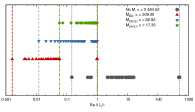
The impact of this preconditioner on the eigenspectrum of the system matrix is illustrated in Figure 1, where we compare the eigenspectra of the preconditioned and actual system matrix. It is clear from the figure that the preconditioner performs very well as far as very large eigenvalues of the initial matrix are concerned as it shifts them to nearly unity. This leads to an overall improvement of the system matrix condition number, as large and small eigenvalues are clearly rescaled differently. Nevertheless, small eigenvalues persist and can potentially continue to hinder the convergence of the iterative solvers. However, the number of these small eigenvalues seems limited in the cases of interest here. Indeed, in the example shown in the Figure with red triangles, there are fewer than $20$ eigenvalues smaller than a factor of $\sim 20$ than the largest one, which, however, span a range of nearly two orders of magnitude. This suggests that we could significantly improve on the condition number of the preconditioned system matrix, if we could scale up these small eigenvalues and do so without affecting significantly the others. This observation leads to the idea of a two-level preconditioner discussed in the next Section.

Figure 1: An approximated spectrum (twenty of the smallest and largest eigenvalues) of an example system matrix derived for the polarisation-sensitive case and preconditioned with different preconditioners. From the bottom to the top, we show the eigenvalues of $\mathbf{A}$, $\mathbf{M}_{BD}\,\mathbf{A}$, and $\mathbf{M}_{2lvl,\{S,D\}}\,\mathbf{A}$, where $\mathbf{M}_{2lvl,\{S,D\}}$ denotes the two-level preconditioners proposed in Section 3.2. The respective condition numbers, $\kappa$, are given in the legend.

3.2 Two-level preconditioners

Let us first consider a numerically efficient preconditioner, which can selectively rescale a set of the smallest eigenvalues of the system matrix. This can be done with a technique called deflation. Deflation has been an active research area in numerical algebra, since the late eighties (see, e.g., Nicolaides (1987) or the recent survey Gutknecht (2012) and references therein) and successfully employed in diverse scientific and industrial contexts. In essence, it aims at deflating the matrix from an unwanted subspace which hinders the convergence of iterative methods. This unwanted subspace is typically the subspace spanned by eigenvectors corresponding to the eigenvalues close to zero of the system matrix (Morgan 1995; Kharchenko & Yeremin 1995; Chapman & Saad 1996). We use a deflation method based on the deflation matrix $\mathbf{R}$(Tang et al. 2009) in our work defined as

$$\mathbf{R}:=\mathbf{I}-\mathbf{A}\,\mathbf{Z}\,\mathbf{E}^{-1}\,\mathbf{Z}^{T}\,,\quad\mathbf{E}:=\mathbf{Z}^{T}\mathbf{A}\,\mathbf{Z}.$$ (11)

Here $\mathbf{I}$ is the identity matrix of size ${{\cal N}_{p}\times{\cal N}_{p}}$, and $\mathbf{Z}$ is a tall and skinny matrix of size ${{\cal N}_{p}\times r}$ and rank $r\,(\ll{\cal N}_{p})$. Matrix $\mathbf{Z}$ is referred to as a deflation subspace matrix, while matrix $\mathbf{E}$ is called a coarse operator. As $\mathbf{A}$ is SPD, so is $\mathbf{E}$. The size of $\mathbf{E}$ is $r\times r$, and its direct factorisation can be easily computed. The columns of $\mathbf{Z}$ are linearly independent and are selected in such a way that they span the subspace, referred to as the deflation subspace, which is to be projected out from any vector it is applied to. That this is indeed the case can be seen noting that $\mathbf{R}\mathbf{A}\mathbf{Z}=\mathbf{0}$. When applied to the case at hand, the deflation subspace is defined to contain the eigenvectors corresponding to small eigenvalues of $\mathbf{A}$. As a result, all these eigenvalues are replaced by zeros in the spectrum of $\mathbf{R}\,\mathbf{A}$, while all the others remain unchanged. In the exact precision arithmetic, $\mathbf{R}$ would potentially be a very efficient preconditioner, as all the steps of any iterative CG-like solver would be orthogonal to the null space of the preconditioned matrix, $\mathbf{R}\,\mathbf{A}$. However, in the finite precision arithmetic, this may not be the case, and the zero eigenvalues are often as bothersome as the small ones due to numerical errors. Another practical problem is that the dimension of the deflation subspace, given by the number of columns of $\mathbf{Z}$, is typically limited for computational reasons. Hence, preconditioners based on deflation are most effective when the system matrix has only few small and outlying eigenvalues.

Both these issues can be overcome by combining a deflation preconditioner with another one. Such combined constructions are referred to as two-level preconditioners. There are numerous prescriptions, both additive or multiplicative, in the literature proposing how to combine two preconditioners. In our work, we use the proposal of Tang et al. (2009) and combine them together with the standard and deflation preconditioners as follows:

$$\mathbf{M}_{2lvl} := \mathbf{M}_{BD}\,\mathbf{R}\,+\,\mathbf{Z}\,\mathbf{E}^{-1}\mathbf{Z}^{T}$$

$$= \mathbf{M}_{BD}\left(\mathbf{I}-\mathbf{A}\,\mathbf{Z}\,\mathbf{E}^{-1}\,\mathbf{Z}^{T}\right)+\mathbf{Z}\,\mathbf{E}^{-1}\,\mathbf{Z}^{T}.\,$$

This corresponds to the ”Adapted Deflation Variant 1” method (A-DEF1) in Tang et al. (2009). We note that this may not be the most obvious choice from a purely theoretical perspective, see Appendix B. However, this is the one, which has proven to be the most robust and efficient in our numerical experiments, and for this reason, we have adapted it in this work.

We note that this new, two-level preconditioner indeed resolves the two problems mentioned before. First,

$$\mathbf{M}_{2lvl}\,\mathbf{A}\mathbf{Z}\,=\,\mathbf{Z},$$ (13)

and therefore the two-level preconditioner rescales all the eigenvalues of $\mathbf{A}$ contained in the deflation subspace defined by $\mathbf{Z}$ to unity. Second, for $\mathbf{Y}^{t}\mathbf{A}\,\mathbf{X}\,=\,\mathbf{0}$,

$$\mathbf{M}_{2lvl}\,\mathbf{A}\mathbf{Y}\,=\,\mathbf{M}_{BD}\,\mathbf{A}\,\mathbf{Y}.$$ (14)

That is, the action of the two level preconditioner, $\mathbf{M}_{2lvl}$, on the eigenvectors of $\mathbf{A}$ orthogonal to the deflation subspace in the sense of the A-norm is equivalent to that of the standard preconditioner, which we have seen in Figure 1 effectively shifts the large eigenvalues towards one. If $\mathbf{Z}$ is defined to include all small eigenvalues of $\mathbf{A}$, the two-level preconditioner will therefore shift both the small and large eigenvalues of $\mathbf{A}$ to the vicinity of one. In practice, the size of the deflation subspace is limited, so this can be achieved only partially. The challenge, therefore, is in a construction of $\mathbf{Z}$ that ensures that the smallest eigenvalues, which are potentially the most troublesome eigenvalues from the point of view of the iterative method convergence, are included and which should be numerically efficient so the performance of this approach is competitive with the standard method. We discuss two different proposals for the latter task in the next Section.

3.3 Deflation subspace operator

In the ideal case, the columns of the deflation subspace matrix, $\mathbf{Z}$, should be made of the eigenvectors corresponding to the smallest eigenvalues of the preconditioned system matrix, $\mathbf{M}_{BD}\,\mathbf{A}$. However these are typically too expensive to compute and, instead, one needs to resort to some approximations.

There are two broad classes of suitable approximation schemes, which are either a priori, and therefore using only the initial knowledge of the problem that we want to solve to construct $\mathbf{Z}$, or a posteriori, which resorts to some explicit precomputation performed ahead of the actual solution. The precomputation can rely on prior solutions of analogous linear systems solved via some iterative algorithm and some simpler preconditioner, as, for instance, $\mathbf{M}_{BD}$ in our case. The preconditioners of this type are clearly useful if the map-making problem with the same system matrix needs to be solved multiple times for different right hand sides, so the precomputation cost quickly becomes irrelevant. This is indeed the case in many practical situations, be it extensive Monte Carlo simulations or posterior sampling algorithms, such as the Monte Carlo Markov Chain approaches, which both are frequently used in CMB data analysis.

In Grigori et al. (2012), we proposed an a priori two-level preconditioner suitable for total intensity observations of the CMB. Below, we first generalise this preconditioner to polarisation-sensitive observations and then introduce a new a posteriori preconditioner.

3.3.1 A priori construction

For the total intensity case, our a priori two level preconditioner is based on the deflation subspace built to include a pixel domain vector of ones, $\mathbf{1_{p}}$. This is because the vector of ones is in the near nullspace of the system matrix, whenever long-term time domain correlations are present. To demonstrate this, let us consider the typical power spectrum of such noise, as given in equation (21). This spectrum displays a characteristic ”$1/f$” behaviour at the low-frequency end, which results in a significant excess of power in this regime. Though more realistic noise spectra typically flatten out at very low frequencies, instead of continuing to increase as $1/f$, the power excess is nevertheless present, as the flattening happens at frequencies much lower than $f_{knee}$. As the noise spectrum corresponds to the eigenvalues of the noise correlation matrix, $\mathbf{N}$, as in equation (4), it is apparent that the eigenvalue of the zero frequency mode is significantly larger than the majority of the other eigenvalues corresponding to the high frequency plateau of the spectrum. Consequently, the zero frequency mode given by a vector of ones in the time-domain, $\mathbf{1_{t}}$, is in the near nullspace of the inverse time-domain correlation matrix, $\mathbf{N}^{-1}$, that is $\mathbf{N}^{-1}\,\mathbf{1_{t}}\,\simeq\,0$. Hence, given that

$$\mathbf{A}\,\mathbf{1_{p}}=\mathbf{P}^{t}\,\mathbf{N}^{-1}\,\mathbf{P}\,\mathbf{1_{p}}=\mathbf{P}^{t}\,\mathbf{N}^{-1}\,\mathbf{1_{t}}\simeq 0,$$ (15)

the pixel domain vector of ones, $\mathbf{1_{p}}$, is expected to be in the near nullspace of $\mathbf{A}$. We can, thus, expect that including this vector in the deflation subspace should result in significant gains in the solver’s convergence, as is indeed borne out by our results discussed in section 4.

We can strive to further accelerate the convergence by employing a richer deflation subspace matrix, $\mathbf{Z}$. In the approach proposed here, we capitalise on the observation that the instrumental noise, $\@vec{\breve{n}},$ is piece-wise stationary. Let us assume that we have a disjoint $K+1$ stationary intervals, $\@vec{d}^{0},\ldots,\@vec{d}^{K}$. Each interval, $\@vec{d}^{j}$, is associated by construction with a unique time domain noise correlation matrix, $\mathbf{T}^{j}$. The deflation matrix, which we denote hereafter as $\mathbf{Z}_{S}$, is built by assigning each of its columns to one of the piece-wise stationary time intervals (Grigori et al. 2012), such that the $j$th column corresponds to the $j$th stationary interval, $\@vec{d}^{j}$. In the case of the total intensity observations for a given pixel, $p$, the elements in the $j$th column define the fraction of the observations of this pixel performed within the $j$th period, $s_{p}^{j}$, as compared to all its observations, $s_{p}$,

$$\begin{array}[]{rclcl}\mathbf{Z}_{S}^{tint}&:=&\begin{pmatrix}\vskip 3.0pt plus 1.0pt minus 1.0pt{\displaystyle\frac{s^{0}_{0}}{s_{0}}}&{\displaystyle\frac{s^{1}_{0}}{s_{0}}}&{\displaystyle\cdots}&{\displaystyle\frac{s^{K}_{0}}{s_{0}}}\\ {\displaystyle\frac{s^{0}_{1}}{s_{1}}}&{\displaystyle\frac{s^{1}_{1}}{s_{1}}}&{\displaystyle\cdots}&{\displaystyle\frac{s^{K}_{1}}{s_{1}}}\\ {\displaystyle\vdots}&{\displaystyle\vdots}&&{\displaystyle\vdots}\\ {\displaystyle\frac{s^{0}_{p}}{s_{p}}}&{\displaystyle\frac{s^{1}_{p}}{s_{p}}}&{\displaystyle\cdots}&{\displaystyle\frac{s^{K}_{p}}{s_{p}}}\end{pmatrix}.\end{array}$$ (17)

We note that each row of $\mathbf{Z}_{S}^{tint}$ represents some partition of unity as $\sum_{j}\,\mathbf{Z}^{tint}_{S}(p,j)\,=\,1$.

In experiments with polarisation, the extra entries of each column, corresponding to Q and U signals, are simply set to $0$, so the deflation subspace matrix for the polarised cases is given by:

$$\begin{array}[]{cccc}\left(\mathbf{Z}_{S}^{pol}\right)&:=&\begin{pmatrix}\vskip 3.0pt plus 1.0pt minus 1.0pt{\displaystyle\frac{s^{0}_{0}}{s_{0}}}&{\displaystyle\frac{s^{1}_{0}}{s_{0}}}&{\displaystyle\cdots}&{\displaystyle\frac{s^{K}_{0}}{s_{0}}}\\ {\displaystyle 0}&{\displaystyle\cdots}&{\displaystyle\cdots}&{\displaystyle 0}\\ {\displaystyle 0}&{\displaystyle\cdots}&{\displaystyle\cdots}&{\displaystyle 0}\\ {\displaystyle\frac{s^{0}_{1}}{s_{1}}}&{\displaystyle\frac{s^{1}_{1}}{s_{1}}}&{\displaystyle\cdots}&{\displaystyle\frac{s^{K}_{1}}{s_{1}}}\\ {\displaystyle 0}&{\displaystyle\cdots}&{\displaystyle\cdots}&{\displaystyle 0}\\ {\displaystyle 0}&{\displaystyle\cdots}&{\displaystyle\cdots}&{\displaystyle 0}\\ {\displaystyle\vdots}&{\displaystyle\vdots}&{\displaystyle\vdots}&{\displaystyle\vdots}\\ {\displaystyle\frac{s^{0}_{p}}{s_{p}}}&{\displaystyle\frac{s^{1}_{p}}{s_{p}}}&{\displaystyle\cdots}&{\displaystyle\frac{s^{K}_{p}}{s_{p}}}\\ {\displaystyle 0}&{\displaystyle\cdots}&{\displaystyle\cdots}&{\displaystyle 0}\\ {\displaystyle 0}&{\displaystyle\cdots}&{\displaystyle\cdots}&{\displaystyle 0}\end{pmatrix}.\end{array}.$$ (19)

This choice essentially implies that we apply no correction to the eigenvectors of the system matrix, which have a non-zero component in the part of the space corresponding to the polarised degrees of freedom. This seems justified given that these are degrees of freedom related to the temperature, which are expected to lead to the smallest eigenvalues. We note for instance that the deflation subspace defined in this way does not include the unit vector, that is a vector of ones for all pixels and all three Stokes parameters but it includes only a vector of ones for the temperature pixels and zero otherwise. This is consistent with equation (15), which implies that this is the latter not the former vector, which generally is in the near null space of $\mathbf{A}$ whenever $1/f$ noise is present. For the unit vector, $\mathbf{1}_{3p}$, and for polarisation-sensitive observations, typically $\mathbf{P}\,\mathbf{1}_{3p}\,\neq\,\mathbf{1_{t}}$, while equality is assumed in the derivation of equation (15). We note that this choice is efficient in improving the condition number of the system matrix, as can be seen in Figure 1, and we test its impact on the convergence of the iterative solvers in Section 5.

The deflation subspace matrix, $\mathbf{Z}_{S}$, constructed in this section can be rather sparse, reflecting that only a small subset of all pixels is typically observed within each stationary period. The sparsity is therefore uniquely given by the definition of the stationary periods and the structure of the pointing matrix and can be predicted ahead of time and used to implicitly construct the preconditioner, which is then applied at each step of the iterative solver. As the number of columns, $r$, of the operator $\mathbf{Z}_{S}$ is tied to the number of stationary periods, it may seem that the size of $\mathbf{A}$ is uniquely predetermined by the data set properties. However, though not completely arbitrary, the number of columns of $\mathbf{A}$ can always be reduced by combining some of the stationary periods together. As we discuss in Section 5.1.2, at least in some cases, such an approach can ensure satisfactory performance at lower numerical cost with fewer columns of $\mathbf{Z}_{S}$. We emphasise that the reduction of the size of $\mathbf{Z}_{S}$ must be performed consistently, and in particular the sum of all elements for each nonzero row of $\mathbf{Z}_{S}$ has to remain equal to $1$ after such an operation is performed. Hereafter, unless stated explicitly, we always take $r=K$.

3.3.2 A posteriori construction

In this case, the deflation subspace matrix, $\mathbf{Z}$, is constructed based on some suitably devised precomputation, which typically yields approximate eigenvectors of the preconditioned system matrix, $\mathbf{M}_{BD}\,\mathbf{A}$. A particularly interesting option, which we focus on here, is when the precomputation consists in solving a similar linear system to the actual one and featuring the same system matrix, $\mathbf{A}$, but potentially different right-hand side, $\@vec{b}^{\prime}$,

$$\mathbf{A}\@vec{x}^{\prime}=\@vec{b}^{\prime}.$$ (20)

Any iterative solver of such systems based on the Krylov subspace methods (see Appendix A) internally derives information about the spectral properties of the system matrix. This information can, therefore, at least in principle, be stored and then re-used in building the deflation subspace matrix (denoted hereafter $\mathbf{Z}_{D}$) of a two-level preconditioner, which could be subsequently applied in the following solves of the same system. We could expect that this approach leads to a two-level preconditioner, which generally is more efficient than any a priori construction, as the coarse space operator constructions is performed using estimates of the true eigenvectors of the matrix.

There are many specific proposals of these constructions in the numerical linear algebra literature, which are specialised for either GMRES (Morgan 1995; Kharchenko & Yeremin 1995; Chapman & Saad 1996; Saad et al. 2000; Parks et al. 2006) or the conjugate gradient method (Erhel & Guyomarc’h 2000; Risler & Rey 2000; Gosselet & Rey 2003). For more details, we refer the reader to Appendix A and the original papers, while we just list the main common steps of these algorithms here. These steps are as follows:

1. Solve the initial linear system (or systems) $\mathbf{M}_{BD}\,\mathbf{A}\,\@vec{x}^{\prime}\,=\,\mathbf{M}_{BD}\,\@vec{b}^{\prime}$ using a Krylov subspace iterative method. As a by-product, we obtain a spectral decomposition of the respective Krylov subspace, see equation (22).

2. Derive approximations of the eigenvalues and eigenvectors of $\mathbf{A}$ by employing the Ritz eigenvalues approach, see equation (25).

3. Select the Ritz eigenvectors, which correspond to eigenvalues with real parts smaller than some given threshold, $\epsilon_{tol}$. (Note that we describe here a more general setting, which does not assume that the matrices are SPD).

4. Construct the deflation subspace matrix as $\mathbf{Z}_{D}:=|\@vec{V}_{1}|\@vec{V}_{2}|\ldots|\@vec{V}_{r}|$, where $(\@vec{V}_{1},\ldots,\@vec{V}_{r})$ denote $r$ eigenvectors selected in the previous step.

5. Construct our two-level preconditioner using $\mathbf{Z}_{D}$.

Unlike the matrix $\mathbf{Z}_{S}$ discussed earlier, $\mathbf{Z}_{D}$ will typically be dense. However, the number of its columns $r$ could essentially be set arbitrarily and be typically determined by a suitable choice of the tolerance threshold, $\epsilon_{tol}$.

We also note that in principle one could imagine that the deflation subspace operator constructed for the current run is subsequently updated with the new information obtained from it before being used for the next run if many map-making runs have to be performed. Thus, it can be potentially used to progressively construct a more efficient coarse operator. From our experience, the additional benefits of such an approach are very quickly becoming minor and come at the cost of a significant extra complexity of the implementation. We have, therefore, not considered this option in this work.

3.4 Cost of application and storing $\mathbf{M}_{2lvl}$

The two-level preconditioners, as defined in equation (3.2), are in general dense. Therefore, in the algorithms proposed here, they are not and not can be constructed explicitly. Instead, we precompute only the matrix $\mathbf{A}\mathbf{Z}$ and the coarse operator, $\mathbf{E}$, which we store in the computer memory. We then apply $\mathbf{M}_{2lvl}$ to a vector as in equation (3.2), performing the matrix vector operations from left to right.

The details of our implementation are given in Appendix C. Once $\mathbf{A}\,\mathbf{Z}$ and $\mathbf{E}$ are available they demonstrate that the operations required by the two-level preconditioner are performed within either deflation or pixel space and are, therefore, subdominant as compared to the time-domain operations, such as noise-weighting, which is involved in the products of the system matrix by a vector and, therefore, needs to be repeated on every iteration. We can, therefore expect that the extra computational cost introduced by these preconditioners are manageable. We confirm this expectation by means of numerical experiments in Section 5 and Appendix C.

4 Numerical experiments

(a)

(b)

(c)

(d)

(e)

Figure 2: Visualisation of the input information used for the simulations (see Sect. 4.1 for more details). Upper row: panels (a-c), hit maps obtained for the grid-like, small circle, and big circle scans, respectively. Bottom row: (d) noise correlations assumed for the stationary intervals and corresponding to different values of the knee frequency $f_{knee}$, (the diagonal, highly dominant element is not shown to emphasise the off-diagonal correlations), (e) an example of the total intensity map of the CMB fluctuations.

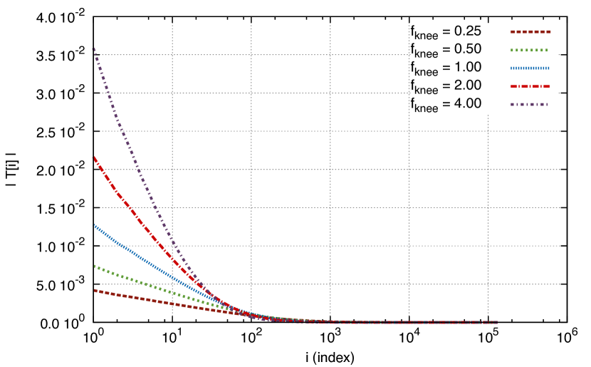
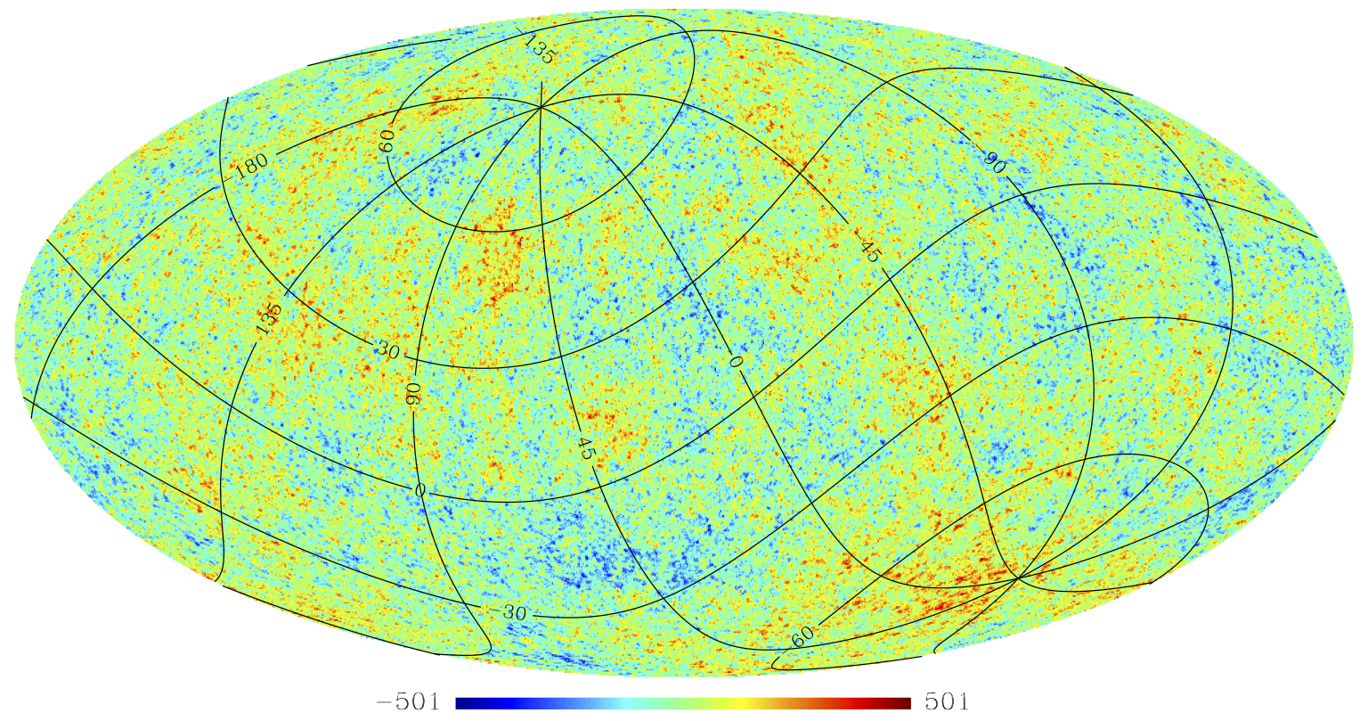
In this section, we present a number of numerical experiments demonstrating that PCG preconditioned by the two-level preconditioners provide an efficient and robust iterative solver for the map-making problem. The numerical experiments have been designed with the following main objectives in mind:

1. To demonstrate that the number of iterations needed to converge that is to reach a given pre-defined magnitude of the residuals, is smaller in the case of the two-level preconditioner than in the case of the standard one.

2. To demonstrate that the two-level preconditioner also leads to important savings in terms of time to solution.

3. To demonstrate that the two-level preconditioner can be implemented for massively parallel computers and in a scalable manner. That is, that it is capable of maintaining its performance and, in particular, fulfils the two first objectives, with an increasing number of processors. This is necessary given the volumes of current and future CMB data sets.

In the following, we discuss the efficiency of the two-level preconditioners with respect to these objective for a range of simulated CMB-like observations with realistic characteristics. In particular, we consider different scanning patterns, sizes of the data set in time- and pixel- domains, noise correlation lengths, etc. We also discuss the role of the bandwidth assumption, which is typically imposed on the Toeplitz matrices used to describe properties of stationary time domain noise, as seen in equation (4). As the reference for all the runs described below, we use the PCG solver with the standard block-diagonal preconditioner, $\mathbf{M}_{BD}$.

4.1 Simulations

The numerical experiments use simulated CMB data sets with characteristics inspired by actual CMB experiments but are kept simple to permit inferences about the impact of their different parameters on the performance of the method. In general, the time ordered data (TOD) is simulated by generating a list of telescope pointings produced for a selected scanning strategy and assigning the respective signals to it, $\mathbf{i}_{p},\mathbf{q}_{p}$, and $\mathbf{u}_{p}$, as read off from the simulated CMB maps. The recovered signals are combined together as in equation (2), added to simulated instrumental noise $\@vec{\breve{n}_{t}}$, and stored as a time domain vector, $\@vec{d}_{t}$.

4.1.1 Scanning strategies

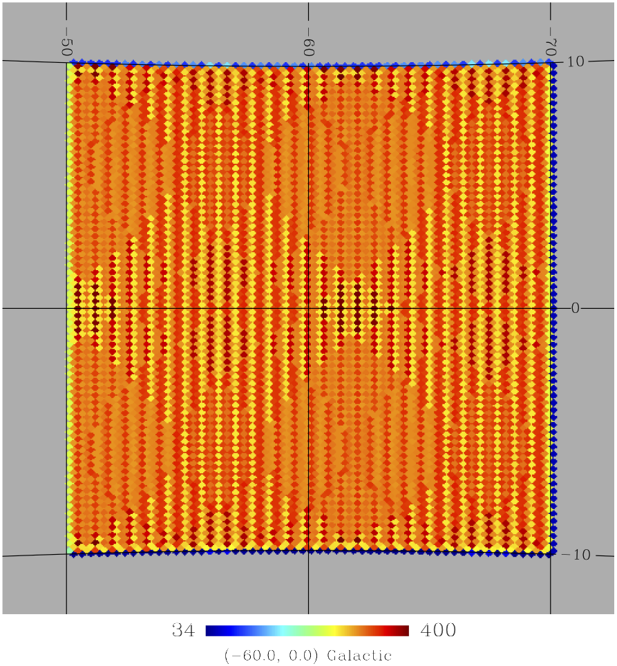
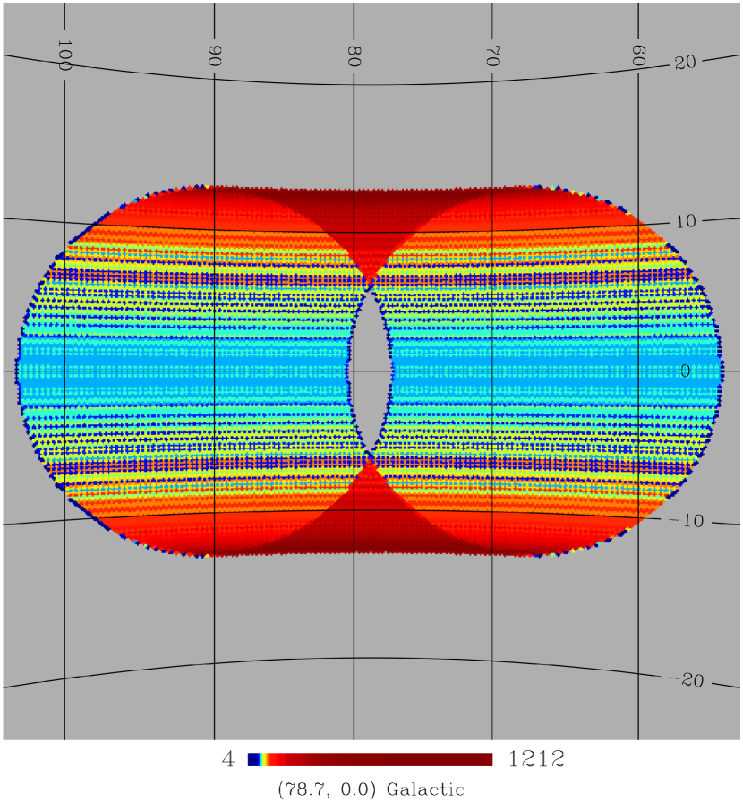
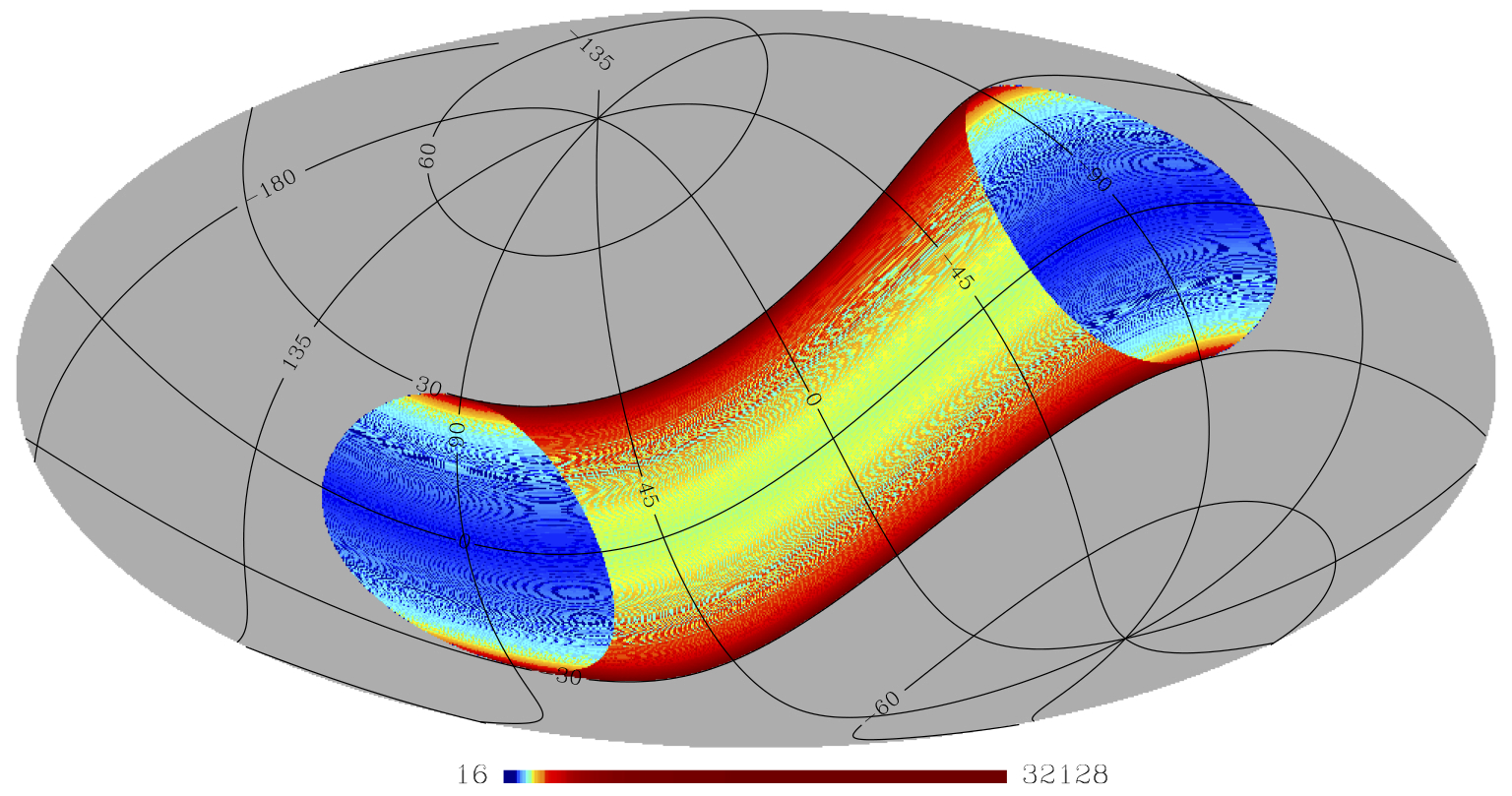
We employ three simplified scanning strategies in our simulations, as listed in Table 1. They correspond to either small-scale or nearly full-sky observations, have different sizes in the time and pixel domains, and have various levels of redundancies present in the scan, as quantifiable by a different distribution of the number of revisits of sky pixels, or a different distribution of the attack-angles in pixels. The studied cases are

1. A grid-like scan in which a patch of $20^{\circ}\times 20^{\circ}$ deg on the sky is observed in turn either horizontally or vertically, as seen in Figure 2a.

2. A scan made of $128$ circles on the sky with the diameter of $15^{\circ}$ deg and centres located along one of the celestial sphere’s great circles, as seen in Figure 2b. Each circle is scanned four times before the experiment moves to the another one.

3. A scan pattern made of $2048$ densely crossing circles, as shown in Figure 2c, which are scanned one-by-one, consecutively, from left to right. The circles have the opening angle of $30^{\circ}$. The time spent on each circle is assumed to be the same. Each circle is scanned $16$ times and sampled $\approx 10^{6}$ times before the experiment switches to another one. As a result of such a procedure, we have a vector of more than two billion observation directions. This scan reflects some of the basic properties of a satellite-like observation.

Table 1: Size of the problem for the different cases analysed.

		# of stationary	# of	# of
Case	Pattern	intervals	pixels	time samples
1	Grid scan	1	7762	$\simeq 1.0\times 10^{6}$
2	Small circles	1	20585	$\simeq 2.0\times 10^{6}$
3	Big circles	2048	998836	$\simeq 2.0\times 10^{9}$

4.1.2 Polariser

We specify a dependence of the orientation of the polariser, $\phi_{t}$, as defined in equation (2), on time, assuming three scenarios.

1. Fast polariser rotation: The polariser is rotated by $45^{\circ}$ deg from one to another pointing along the scan direction.

2. Medium rotation: We change the polariser angle by $45^{\circ}$ deg after each scan of one circle (for the circular scans) or after changing of direction of scanning (for the grid-like scan).

3. Slow rotation: In this case we repeat the full scan four times before changing the polariser angle by $45^{\circ}$ deg. As a consequence, the time domain is four times larger than the ones listed in Table 1.

4.1.3 CMB signal

Theoretical power spectra have been calculated using the CAMB package (Challinor & Lewis 2011) assuming the concordance model parameters (Planck Collaboration et al. 2013). They have subsequently been convolved with a fiducial symmetric Gaussian instrumental beam of FWHM $10$ arcminutes and used to simulate a Gaussian realisation of the CMB map using the synfast routine from a HEALPix (Górski et al. 2005) with a HEALPix resolution parameter set to ${\cal N}_{side}=512$.

4.1.4 Noise

We have simulated the noise contribution, $\@vec{\breve{n}_{t}}$, as a Gaussian realisation of a piece-wise stationary noise composed of an uncorrelated white noise and correlated $1/f$ components with the power spectrum density for each of the stationary pieces that are that are parametrized in the usual manner as

$$P(f)=\sigma^{2}\,t_{samp}\left(1+\left(\frac{f_{knee}}{f}\right)^{2}\right).$$ (21)

Here, $\sigma^{2}$ defines the white noise level, $t_{samp}$ is the sampling interval, and $f_{knee}$ – the knee frequency of the spectrum. For definiteness, we used $\sigma^{2}=8.8\,10^{-10}$K${}_{CMB}^{2}$ for a single observation noise variance – a value roughly corresponding to a typical noise level of current bolometric detectors.

For the two smaller scans, cases 1 and 2 in Table 1, we have assumed that the noise is stationary over the entire period of the observation, while stationary intervals correspond to the time spent scanning each circle for the largest experiment (case 3). This implies that noise correlations are then present only between the samples corresponding to the same circle, and the resulting (inverse) noise covariance, as seen in equation (4), is composed of as many diagonal blocks, as circles, that is up to $2048$. This is in contrast with cases 1 and 2, where there is only one Toeplitz block.

For any stationary interval, noise correlations may exist between any two of its samples however distant they are. This would correspond to full dense Toeplitz blocks of the (inverse) noise correlation matrix, $\mathbf{N}^{-1}$. It is, however, frequently assumed that the correlations are zero if the time lag between the samples exceeds some correlation length, $\lambda_{T}$. If this is indeed the case, the Toeplitz blocks of $\mathbf{N}^{-1}$ are band-diagonal with a half bandwidth set by $\lambda_{T}$. In our experiments for definiteness, we set this parameter to be $\lambda_{T}=2^{13}$, unless it is explicitly stated otherwise. We discuss the role and importance of this parameter on the efficiency of the iterative solvers in Section 5.

4.2 Experimental setup

We evaluate performance of our two-level solver on NERSC’s supercomputer Hopper, based on a Cray XE6 system. Hopper is made up of $6384$ compute nodes with each node composed of two twelve-cores AMD MagnyCours ($2.1$ GHz), with a peak performance of $201.6$ Gflops per node and $1.288$ Peta-flops for the entire machine. The nodes are connected with Cray’s Gemini high performance interconnect network.

For the tests we use our own parallel code written in C++, which uses a multithreaded version of Intel’s Math Kernel Library for calculation of the Fast Fourier Transforms and for dense linear algebra. We use Intel Compiler version 12.1.4.

The code is fully parallelised using a distributed-memory programming model with help of the MPI (Message Passing Interface) library. In addition, some routines in our code and the MKL library used in our implementation allow us to exploit multithreading. This is done by assigning each MPI (distributed memory) process to a single multicore processor and then by capitalising on its multicore structure with OpenMP threads, which is managed via calls to the OpenMP library. On Hopper, we use four MPI processes per compute node and six OpenMP threads per MPI process. Consequently, a run using $2048$ MPI processes typically uses up to $2048\times 6=12,288$ cores. Details of our implementation and the assumed data layout are given in section C.

5 Results and discussion

5.1 Convergence comparison

(a) Polarisation case 1

(b) Polarisation case 2

(c) Polarisation case 3

Figure 3: Convergence of the preconditioned CG solver applied to the simulated data, as described in Section 5.2. Different line styles correspond to different sizes of the problem, while different colours correspond to the three different types of preconditioners: red for the standard block preconditioner $\mathbf{M}_{BD}$, and green and blue for the two-level preconditioners, $\mathbf{M}_{2lvl,S}$ and $\mathbf{M}_{2lvl,D}$, respectively. In the legend, $K$ corresponds to the number of stationary intervals in the time domain data and dim$(\mathbf{Z})$ denotes the number of columns in the deflation subspace operator, $\mathbf{Z}$. For the a posteriori preconditioner, $\mathbf{M}_{(2lvl,D)}$, dim$(\mathbf{Z})$ is the number of eigenvalues, which fulfill the condition ${\rm Re}|\lambda_{i}|<\epsilon_{tol}=0.2$.

(a) Rectangular scan.

(b) Small circles scan.

Figure 4: Convergence of the PCG solver of the CMB map-making problem for two different scanning strategy. Different types of lines correspond to different versions of the Toeplitz matrix used in the simulation, as described by the parameter $f_{knee}$. Different colours correspond to the two different types of preconditioners: red for the standard block preconditioner $\mathbf{M}_{BD}$ and green for the two-level preconditioner $\mathbf{M}_{2lvl,D}$ whose coarse space $\mathbf{Z}_{D}$, is made of approximated eigenvectors corresponding to small eigenvalues $\lambda_{i}$ of $\mathbf{M}_{BD}\,\mathbf{A}$. dim$(\mathbf{Z})$ denotes the number of columns in the deflation subspace operator $\mathbf{Z}_{D}$ which is the number of eigenvalues with $({\rm Re}|\lambda_{i}|<\epsilon_{tol}=0.3).$

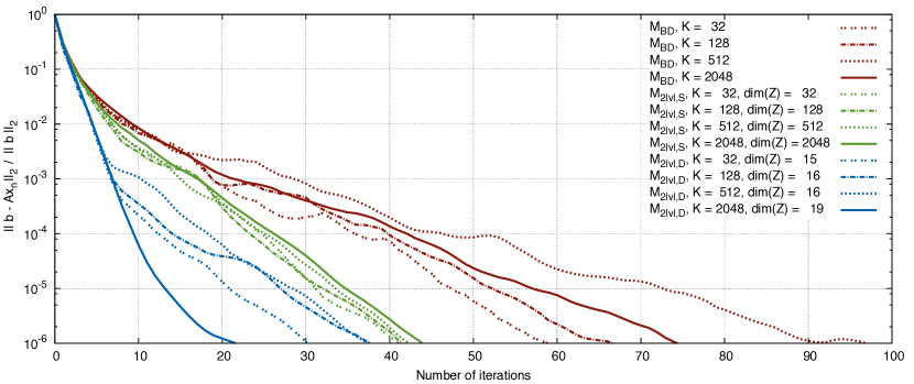
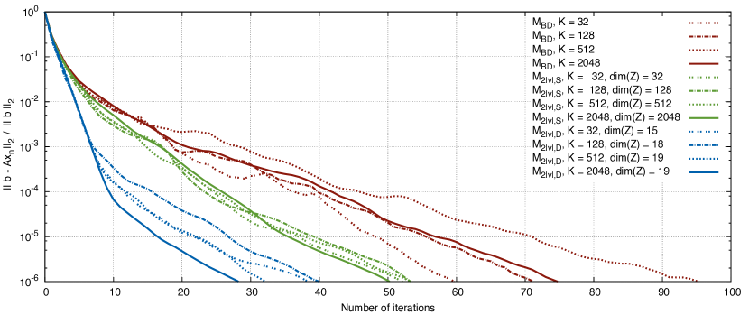
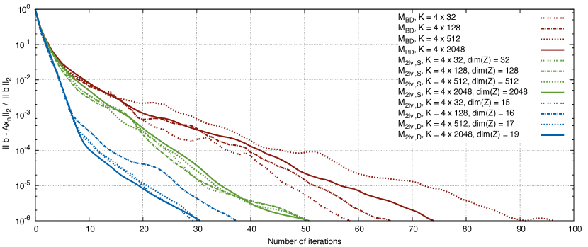
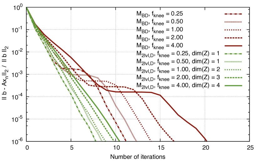
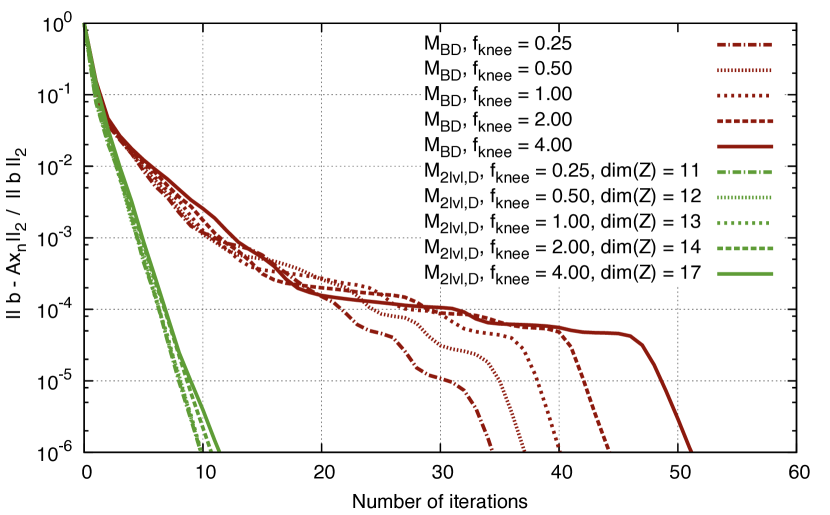
Figure 3 shows the magnitude of the relative error of the solution defined as $(||\@vec{b}-\mathbf{A}\,\@vec{x}_{i}||_{2}/||\@vec{b}||_{2})$ as a function of the number of iterations for the standard and two two-level preconditioners: a priori and a posteriori. The results shown here are derived for the scanning strategy referred to as case three in Section 4.1.1 and the different panels correspond to the three variants for polariser dynamics, as described in Section 4.1.2. In each panel, we show results for different lengths of the time domain data, varying the number of assumed sky circles from $32$ to $2048$. For cases 1 and 2 of the polariser rotation, each circle corresponds to a stationary interval, and we alternate the value of $f_{knee}$ between $0.5$Hz and $1$Hz for odd and even circles, respectively. For case 3, each circle is scanned four times, each time with a different $f_{knee}$ alternating as above. The number of stationary intervals, $K$, is marked in each panel for each of the studied cases. For the a priori construction, $K$ defines the dimension of the deflation subspace and the number of columns of $\mathbf{Z}_{S}$. The a posteriori operator, $\mathbf{Z}_{D}$, is built from approximated eigenvectors, which are selected assuming $\epsilon_{tol}=0.2$. The number of these eigenvectors is given by ${\rm dim}\,(\mathbf{Z})$, as displayed in each panel.

In terms of the number of iterations needed to reach some nominal precision, assumed hereafter to be $10^{-6}$. It is apparent from the plots that the two-level preconditioners outperform the standard one by as much as twice for the a priori two-level preconditoner and a factor of $3.5$ for the a posteriori one. This confirms the theoretical expectations from Section 3.2.

Clearly, both two-level preconditioners offer important performance gains. However, these are more modest compared to those found in Grigori et al. (2012), who reported typical reduction in the number of iterations by as much as a factor of $6$. We attribute this to two facts. First, the bandwidth of the Toeplitz matrices assumed in this work was shorter than what was used in the previous work. Second, the long-time scale noise correlations are more important in the case of total intensity, as studied in Grigori et al. (2012), than in the polarised case, as considered in this work. We elaborate on these issues in the following sections.

(a) With polarisation (Case 2)

(b) No polarisation

Figure 5: Convergence of the CG solver preconditioned with the two-level a priori precondtioner for the scan made of $K=1024$ big circles. Green lines correspond to the solutions obtained using the deflation subspace matrix, $\mathbf{Z}_{S}$, with a progressively lower rank, which is given by ${\rm dim}(\mathbf{Z})$ in the legend. Red curves depict the solution with the standard preconditioner, $\mathbf{M}_{BD}$.

5.1.1 Convergence rate and low frequency noise correlations

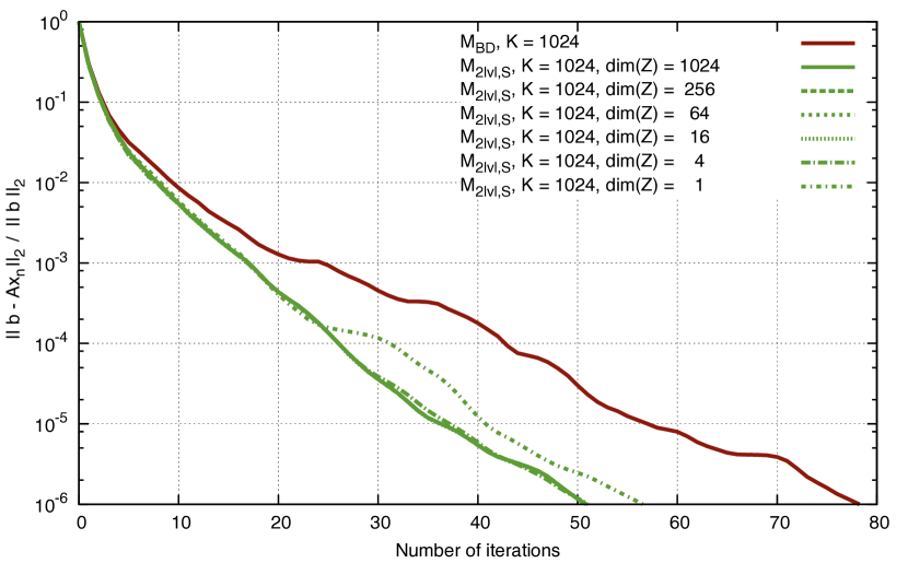
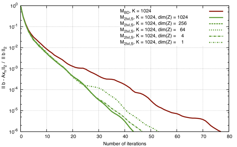
We illustrate the dependence on a level of the noise correlations in Figure 4, which shows the convergence of the preconditioned CG solver for several different data sets that correspond to different values of the parameter $f_{knee}$. In the cases shown in the figure, we used simulations with scanning characteristics that correspond to cases $1$ and $2$ and, therefore, assume only one stationary period for the entire scan as seen in Table 1. In the plot, red curves show the results of the runs with the block diagonal preconditioner. It is clear that the convergence of the block diagonal preconditioner depends very strongly on the value of $f_{knee}$, whenever the required convergence precision is better than $\sim 10^{-4}$. This is around this level that the relative residuals reach typically a plateau and continue their decrease only once it is over. The length of the plateau depends on $f_{knee}$ and so does the number of iterations needed to reach our nominal precision level of $10^{-6}$.

This plateau in the convergence of iterative methods is usually attributed to the presence of small eigenvalues in the spectrum of the system matrix, $\mathbf{M}_{BD}\,\mathbf{A}$ (see e.g. Morgan (1995); Kharchenko & Yeremin (1995); Chapman & Saad (1996); De Gersem & Hameyer (2001)). In our case, the presence of small eigenvalues depends on the level of the noise correlations, as does the length of the stagnation phase, as indeed observed empirically. As our two-level preconditioners have been designed expressly to deal with the effects due to small eigenvalues, we expect that they should be able to help with the convergence slow-down as seen for the standard preconditioner. This is indeed confirmed by our numerical results shown in Figure 4, where green lines show the results obtained with the two-level a posteriori preconditioner.

The upshot of these considerations is that the overall performance gain expected from the two-level preconditioners will strongly depend on the assumed noise properties. We point out that the dimension of the deflation subspace operator, $\mathbf{Z}_{D}$, used in these runs increases with an increasing value of $f_{knee}$. This is because the number of small eigenvalues of $\mathbf{M}_{BD}\,\mathbf{A}$ also increases, and more columns of $\mathbf{Z}_{D}$ are needed to correct for them. This manifests the adaptive character of this version of the two-level preconditioner and should be contrasted with the a priori one, for which the dimension of $\mathbf{Z}_{S}$ would have been kept constant in all runs and equal to $1$. This would unavoidably result in its inferior performance. We note that we recover a gain of a factor of $5$ between the standard and two-level preconditioners for the largest value of $f_{knee}$ and case $2$ scanning strategy, which is close to the results reported in Grigori et al. (2012).

We emphasise that the number of small eigenvalues does not depend only on the value of $f_{knee}$, but also on where the sky signal resides in the frequency domain (see Appendix D for an analogous argument in a somewhat different context). For fixed $f_{knee}$ the number of small eigenvalues increases if the signal shifts towards the smaller frequencies (as a result, for instance, of a decreasing scan speed). Consequently, both these factors play a role in determining what gain one can expect from applying the two-level preconditioner.

5.1.2 Convergence rate and the deflation space dimension

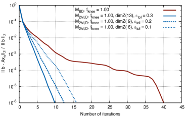
As is evident from the discussion above, the rank of the deflation subspace operator, $\mathbf{Z}$, is yet another parameter with a potentially crucial impact on the performance of the two-level preconditioners. We could expect that increasing the operator’s size has to translate directly into a faster convergence, as it can carry information about more peculiar eigenvalues of the system matrix. This expectation is indeed supported by our numerical experiments. However, we also find that the gain quickly decreases with growing dimension of the deflation space. This is demonstrated in Figure 5 for the a priori preconditioner and in Figure 6 for the a posteriori one. In an extreme case, as shown in the former figure, nearly the entire gain from the two-level construction is already obtained assuming a one dimensional deflation subspace. This single eigenvalue is related to the overall offset of the recovered map, as discussed in Sect. 3.3.1. For fast, well-connected scan speeds and weak noise correlations, it may be sufficient to take care of this major small eigenvalue. This is indeed the case in the example shown in Figure 5.

The dimension of the deflation subspace also has important consequences for the computational cost of the application of the preconditioner. Its adopted value should be ideally a result of a trade-off between these two effects: the expected decrease of the number of iterations and the expected increase in the calculation time per iteration. We discuss the performance in terms of algorithm runtime in the next section.

Figure 6: Convergence of PCG solver preconditioned with the two-level a posteriori preconditioner computed for the small-circles scan with $K=128$ circles and $f_{knee}=1.0$. Blue lines correspond to the solutions obtained with the deflation subspace operator, $\mathbf{Z}_{D}$, with different ranks as defined by the number of approximated eigenvectors with eigenvalues smaller than $\epsilon_{tol}$, as indicated in the legend. Red curve shows the solution with the standard preconditioner, $\mathbf{M}_{BD}$.

Figure 7: Convergence of PCG solver of the simulated CMB map-making problem with the same noise power spectrum but for different lengths of the imposed band limit and for the three preconditioners considered here.

5.1.3 Convergence rate and the bandwidth of the inverse noise correlation matrices

In the remainder of this section, we discuss the role of the Toeplitz matrix bandwidth $\lambda_{T}$, which has been assumed to be fixed in all our numerical tests presented so far with a value of $\lambda_{T}=2^{13}$. The importance of this parameter for the total computational time needed to estimate a map is generally recognised and well known (e.g., Cantalupo et al. 2010). It stems from the fact that the calculation of a product of the inverse noise matrix, $\mathbf{N}^{-1}$, by a time-domain vector is one of the main operations, which needs to be performed recurrently, while solving for the map estimate. At the very best, this cost can be brought down to ${\cal O}({\cal N}_{T}\,\log\,\lambda_{T})$, where ${\cal N}_{T}$ is the length of the stationary interval, but even then it still constitutes a significant, and often dominant, fraction of the entire run-time of the map-making solver (Cantalupo et al. 2010). It is, therefore, desirable to select as small a value of $\lambda_{T}$ as possible.

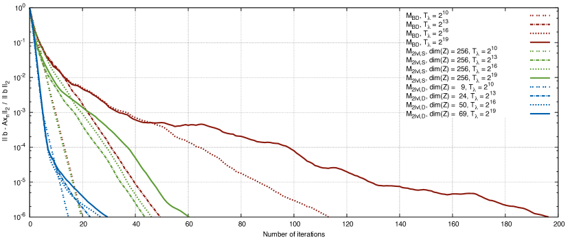
However, a value of $\lambda_{T}$ generally also has a direct impact on the number of iterations needed to converge to the solution. This observation, which is less broadly recognised, is illustrated in Figure 7. For the standard preconditioner, we can see that changing the bandwidth can lower the number of iteration by as much as a factor of $10$. Combined with the gain in computation time per iteration, as mentioned above, this may seem to suggest that this is the parameter one should focus on while optimising any map-making code performance. We argue that though it is clearly very important, the gain in terms of number of iterations, which can be obtained in practice from manipulating the value of $\lambda_{T}$ is quite limited, and does not supersede the gain, which can be achieved thanks to our preconditioners.

The restriction here is due the affect a too small value of $\lambda_{T}$ may have on the quality of the estimated map. A discussion of this issue is presented in Appendix D, where we also discuss parameters playing a role in defining the appropriate value for $\lambda_{T}$. We note that such a critical value of $\lambda_{T}$ is generally a result of a trade-off between acceptable loss of precision and code performance. Moreover, determining it may not be trivial, in particular, for complex scanning strategies. These problems should be contrasted with the preconditioning techniques discussed in this paper, which attempt to speed up the calculation without any impact on the solution.

For the cases shown in Figure 7, the a posteriori preconditioner delivers an order of magnitude improvement in terms of the number of iterations over the run based on the application of the standard preconditioner with $\lambda_{T}=2^{19}$. This is comparable to the gain achieved by simply decreasing $\lambda_{T}$ by a factor of $2^{9}=512$. However, the final bandwidth, if adopted, would affect the quality of the produced map. Indeed, in the examples studied here, the value of $\lambda_{T}$ should be equal to larger than $2^{13}$ to ensure its high precision. The two-level preconditioners yet again deliver competitive and robust performance here with a gain of a factor $2.5$ over the standard run with $\lambda_{T}=2^{13}$ and do so without compromising the quality of the solution.

For the two-level preconditioners, the dependence of the number of iterations on $\lambda_{T}$ is also much weaker than in the standard case, and, hence, the major driver for keeping the bandwidth as small as possible in this case is the need to minimise the overall time of the computation, as we discuss in the next section.

(a) Weak scaling.

(b) Strong scaling.

Figure 8: Total time spent in the iterative solver for the standard, block-diagonal preconditioner, $\mathbf{M}_{BD}$, and the two variants of our new two-level preconditioner, $\mathbf{M}_{2lvl}$, plotted as a function of the number of MPI process used for the computation. The results of the weak scaling tests, i.e., in which problem size is increased proportionally to the number of employed MPI processes, are shown in the left panel, while the results of the tests with a fixed size of the problem, so called strong scaling, are depicted in the right panel. Dashed lines show the cost of the construction of the preconditioners.

(a) Weak scaling.

(b) Strong scaling.

Figure 9: Solid lines show the speedups achieved by the methods with the two-level preconditioners, $\mathbf{M}_{2lvl,S}$ and $\mathbf{M}_{2lvl,D}$, with respect to the traditional solver with the block diagonal preconditioner, $\mathbf{M}_{BD}$, while dotted and dashed lines show the speedups obtained on different stages of the solution. The panels show weak (left), and strong (right), scaling, respectively.

5.2 Runtime comparison

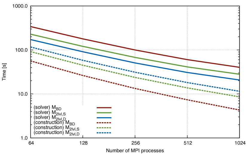
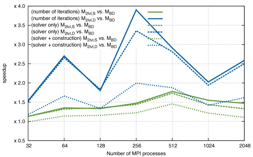
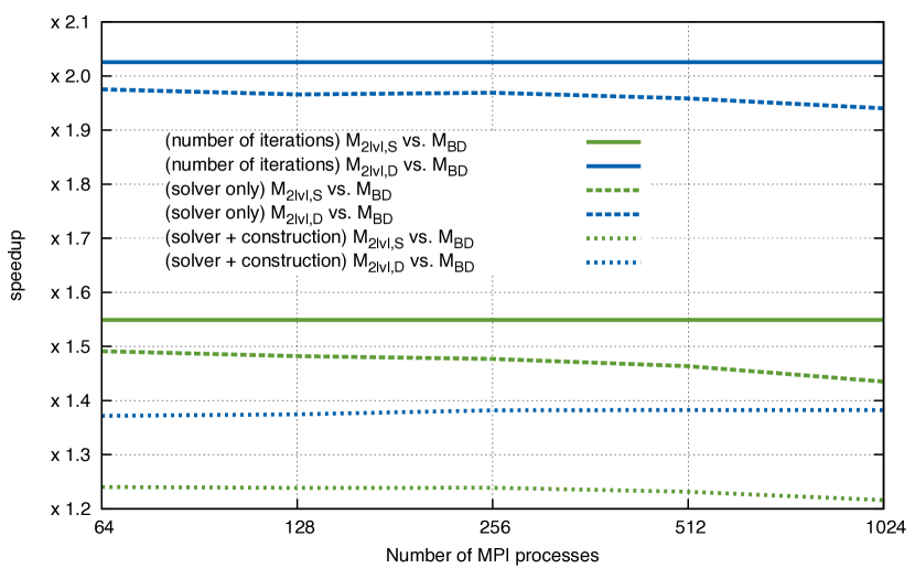
In this section, we evaluate the performance of the proposed methods in terms of the time needed for solving the map-making problem by separately measuring the time required by each solver to construct the preconditioner and time spent on the iterative method. These results are summarised in Figures 8 and 9, showing the runtime results and achieved speed-ups, respectively.

We emphasise that we have not performed any tuning of the deflation subspace dimension for these runs, which could further improve performance of the two level preconditioners. We also use the standard value for $\lambda_{T}(=2^{13})$ and a moderate value of $f_{knee}(=1Hz)$. As was shown earlier, these two parameters affect the performance of the standard preconditioner significantly more than that of the two-level ones, so the timings shown here should be seen as rather conservative.

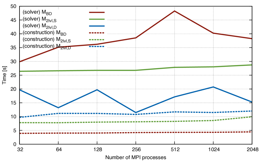
Figure 8 shows the timing results. Dashed lines depict times needed to construct the preconditioners, and solid lines display time required by the iterative solver to converge to the nominal tolerance of $10^{-6}$. These timings are shown as a function of the number of MPI processes used for the runs. The left panel shows the so-called weak scaling, when the size of the problem increases proportionally to the number of MPI processes. The right panel shows the strong scaling when the problem size is fixed. In our weak scaling performance tests, we assign a single stationary interval and, therefore, a single diagonal block of $\mathbf{N}^{-1}$ to a single MPI process. Increasing the number of MPI processes concurrently increases the length of the data set and the number of stationary intervals. In the strong scaling tests, we fix the number of circles to $1024$ and distribute the data evenly among the available processes, by assigning multiple blocks to one MPI process. This limits the number of processes which can be used in these tests to $1024$, and, therefore, the number of cores to $6144$.

The results shown in Figures 8 and 9 demonstrate that the two-level preconditioners fare better in all cases and often much better than the standard one with the a posteriori preconditioner found to be consistently the best. The speedups over the standard case can be as large as $3.5\sim 4$ and tend to be on average around $\sim 2.5$ for the a posteriori option and on the order of $1.5$ for the a priori one. The two-level a posteriori preconditioner shows superior performance even when the preconditioner construction time is taken into account, despite its construction taking the longest out of the three options considered in this work. The respective speedups are consequently lower and typically around $\sim 2$ for the a posteriori preconditioner. For the a priori preconditioner the speedup is minor but still consistently better than $1$. Importantly, if successive linear systems with the same system matrix but different right-hand sides need to be solved, the cost of building the preconditioner needs to be incurred only once, and we can eventually recover the speedups of $\sim 3.5$ and $\sim 1.5$ for the a posteriori and a priori two-level preconditioners, respectively.

We note that the limitations on the speedups obtained here are not due to our numerical implementation but stem from the method itself. This can be seen by comparing the speedups achieved by the code without the precomputation time (dashed lines in Figure 9) with that estimated solely on the basis of the improvement in the number of iterations needed for the convergence (0solid lines). Both these speedups are found to be close, even though the latter estimates do not account for the extra time needed to apply the more complex two-level preconditioners. We conclude that there is little we could gain by optimising our code at this time. This is supported by the discussion of the overall time breakdown between specific operations given in Appendix C.

The results also show very good scaling properties of the proposed two level algorithms. Indeed, the time needed to solve a fixed-size problem decreases nearly inversely proportionally to the number of employed MPI processes (strong scaling), while it remains essentially constant if the problem size grows in unison with the number of the process (weak scaling). This potentially shows that these algorithms eventually can be run on a very large number of distributed compute nodes, as required by forthcoming huge data sets and can do so without significant performance loss.

6 Conclusions

We have proposed, implemented, and tested two new iterative algorithms suitable for solving the map-making problem in the context of scanning, polarisation-sensitive CMB experiments. These algorithms are based on the PCG method supplied with new two-level preconditioners, which are constructed either on the basis of global properties of the considered data set, referred to as a priori preconditioners, or with help of some specialised precomputation, a posteriori preconditioners. This work, therefore, generalises the considerations of Grigori et al. (2012) in two directions. First, it considers polarisation-sensitive observations. Second, it studies a broader class of preconditioners.

With the help of numerical experiments, we have demonstrated that the proposed solvers consistently lead to better performance than the standard, block-diagonal preconditioners, which define the state-of-the art in the field. In particular, we find that the a posteriori preconditioner can decrease the number of iterations needed for convergence by as much as a factor of $5$, and the overall runtime by as much as a factor of $3.5$. The gains obtained with the a priori preconditioner are more modest but still interesting given how straightforward its implementation is.

We have studied the dependence of the performance of the proposed preconditioners on some of the parameters defining CMB data sets. In particular, we have found that the performance of the new preconditioners deteriorates only slowly when increasing the bandwidth of the inverse noise correlations, in contrast with the performance of standard preconditioners. This permits us to avoid a subtle and difficult trade-off between calculation quality and speed, which is inherently present in the latter case. Indeed, with the two-level preconditioners we can opt for a conservatively high value of the bandwidth, evading any danger of compromising the quality of the estimate, while retaining the computational efficiency.

Throughout this work, we have assumed that the time-domain noise covariance has a block-diagonal structure with Toeplitz blocks. The proposed approaches can, however, be applied to more complex noise models as long as the noise weighting procedure, a prerequisite also required by the standard approach, is computationally feasible. This applies to noise models obtained by a marginalization of unwanted systematic contributions, as discussed in Stompor et al. (2002). As these more complex noise models will typically require more computations, the overhead due to the application of the two-level preconditioners will be relatively smaller and their relative performance compared to the standard method better. Further gains could be expected if these more complex noise models result in some near degeneracies of the system matrix. This may affect the performance of the standard approach to a larger extent than that of the two-level ones.

Appendix A Background on Krylov subspace iterative methods

In this Appendix, we provide a brief overview of Krylov subspace iterative methods, as well as an approach for approximating eigenvectors of a matrix. Broader background of these techniques can be found in, e.g., Golub & Van Loan (1996) and Saad (2003). Approximations of eigenvectors/eigenvalues of a matrix in the context of deflation techniques are discussed in e.g., Morgan (1995); Chapman & Saad (1996). Havé et al. (2013) gives a recent example of applications of all these techniques in the context of preconditioners of linear systems.

There are several different classes of iterative methods for solving the linear system of equations,

$$\mathbf{B}\,\@vec{x}=\@vec{b},$$

where $\mathbf{B}$ is a real $n\times n$ matrix, $\@vec{b}$ is the right hand side vector of dimension $n$, and $\@vec{x}$ is the sought of solution vector of dimension $n$. Among those, Krylov subspace methods are the most efficient and popular ones. They belong to a more general class of projection methods, which start from an initial guess $\mathbf{x}_{0}$ and, after $m$ iterations, find an approximate solution, $\@vec{x}_{m}$, from the affine subspace $\mathbf{x}_{0}+\mathcal{K}_{m}$, which fulfills the Petrov-Galerkin condition,

$$\mathbf{b}-\mathbf{B}\mathbf{x}_{m}\perp\mathcal{L}_{m},$$

where $\mathcal{K}_{m}$ and $\mathcal{L}_{m}$ are some appropriately defined, method-dependent, $m$-dimensional subspaces of $\mathbb{R}^{n}$.

For the Krylov subspace methods, $\mathcal{K}_{m}$ is defined as

$$\mathcal{K}_{m}(\mathbf{B},\@vec{r}_{0})=span\left\{\@vec{r}_{0},\mathbf{B}\@vec{r}_{0},\mathbf{B}^{2}\@vec{r}_{0},\ldots,\mathbf{B}^{m-1}\@vec{r}_{0}\right\},$$ (22)

where $\@vec{r}_{0}$ is the initial residual, i.e., $\@vec{r}_{0}:=\@vec{b}-\mathbf{B}\,\@vec{x}_{0}$. It is referred to as the Krylov subspace of dimension $m$. A Krylov subspace method therefore approximates the solution as

$$\@vec{x}_{m}=\@vec{x}_{0}+p_{m-1}(\mathbf{B})\,\@vec{r}_{0},$$

where $p_{m-1}$ is a polynomial of degree $m-1$. While all Krylov subspace methods are based on the same polynomial approximation, different choices of the subspace $\mathcal{L}_{m}$ give rise to different variants of the method, such as a conjugate gradient (CG), or general minimal residual method (GMRES) (Saad & Schultz 1986).

In particular, the GMRES algorithm employs the so-called Arnoldi iterations (see algorithm 1) to build an orthogonal basis of the Krylov subspace. These produce the orthonormal basis, $\mathbf{W}^{\left(m\right)}=|\@vec{w}_{1}\,|\@vec{w}_{2}\,|\ldots\,|\ \@vec{w}_{m}|$, of the Krylov sub-space together with a set of scalar coefficients, $h_{ij}$, (where $i,j=1,\dots,m$ and $i\leq j+1$) plus an extra coefficient, $h_{m+1,m}$. The first group of the coefficients can be arranged as a square matrix of rank $m$, called $\mathbf{H}^{\left(m\right)}$, with all elements below the first sub-diagonal equal to $0$. A matrix with such structure is referred to as an upper Hessenberg matrix. It can be shown (e.g., Golub & Van Loan 1996) that there exists a fundamental relation between all these products of the Arnoldi process, which reads

$$\mathbf{B}\,\mathbf{W}_{m}\,=\,\mathbf{W}_{m}\,\mathbf{H}_{m}\,+\,h_{m+1,m}\,\@vec{w}_{m+1}\@vec{e}^{T}_{m}.$$ (23)

Here, $\@vec{e}_{m}$ is a unit vector with $1$ on the $m$th place.

Algorithm 1 Basic Arnoldi Algorithm

0:  $\@vec{r}_{0}$, $\@vec{w}_{1}={\@vec{r}_{0}}/{||\@vec{r}_{0}||}$

1:  for $j=1\to m$ do

2:     for $i=1\to j$ do

3:        $h_{i,j}=(\mathbf{B}\@vec{w}_{j},\@vec{w}_{i})$

4:     end for

5:     $\@vec{v}_{j}=\mathbf{B}\@vec{w}_{j}-\sum\limits_{i=1}^{j}h_{i,j}\@vec{w}_{i}$

6:     $h_{j+1,j}=||\@vec{v}_{j}||_{2}$

7:     $\@vec{w}_{j+1}=\@vec{v}_{j}/h_{j+1,j}$

8:  end for

The eigenpairs of the matrix $\mathbf{H}_{m}$ are commonly referred to as Ritz eigenpairs. They can be straightforwardly computed thanks to the Hessenberg structure of the matrix and its moderate size, which is given by the size of the Krylov space and therefore by the typical number of the iterations needed to solve the system. This is in the CMB applications of the order of ${\cal O}(100)$. By denoting these eigenpairs as $(\@vec{v}_{i},\lambda_{i})$, we can therefore write

$$\mathbf{H}_{m}\,\@vec{v}_{i}\,=\,\lambda_{i}\,\@vec{v}_{i}.$$ (24)

From Eq. (23) for every eigenvector, $\@vec{v}_{i}$, of $\mathbf{H}_{m}$, we find that

$$\mathbf{B}\,\mathbf{W}_{m}\,\@vec{v}_{i}\, = \,\mathbf{W}_{m}\,\mathbf{H}_{m}\,\@vec{v}_{i}\,+\,h_{m+1,m}\,\@vec{w}_{m+1}\,\@vec{e}^{\dagger}_{m}\,\@vec{v}_{i}$$ (25)

$$= \,\lambda_{i}\,\mathbf{W}_{m}\,\@vec{v}_{i}\,+\,h_{m+1,m}\,\@vec{w}_{m+1}\,\@vec{e}^{\dagger}_{m}\,\@vec{v}_{i}.$$

Consequently, if $h_{m+1,m}=0$, then every eigenvector of $\mathbf{H}_{m}$ defines an eigenvector of $\mathbf{B}$ given by $\@vec{y}_{i}:=\mathbf{W}_{m}\,\@vec{v}_{i}$, both of which have the same corresponding eigenvalue, $\lambda_{i}$.

If $h_{m+1,m}$ is not zero, but is small, as it is usually the case if the solver is converged with sufficient precision. The pairs $(\@vec{y}_{i},\lambda_{i})$ then provide a useful approximation of the $m$ true eigenvalues of $\mathbf{B}$, and the magnitude of the last term on the right hand side of Eq. (25) serves as an estimate of the involved error.

In our construction of the a posteriori preconditioner, we take $\mathbf{B}=\mathbf{M}_{BD}\mathbf{A}$ and apply the algorithm described above to calculate the set of the vectors, $\@vec{y}_{i}$, from which we subsequently select the vectors used to build the deflation subspace operator, $\mathbf{Z}_{D}$.

Though the specific approach described here relies on the GMRES solver, we note that a similar construction can be performed using the CG technique as elaborated on, for instance, in Erhel & Guyomarc’h (1997).

Appendix B Alternative construction of a two-level preconditioner

A two-level preconditioner can be constructed in a different way than what is proposed in Section 3.2. One potentially promising alternative, which stands out from a theoretical point of view, can be derived from the ’Adapted Deflation Variant 2’ method (A-DEF2) of Tang et al. (2009) that renders the following expression,

$$\mathbf{M}_{2lvl,}^{(alt)}:=\mathbf{R^{T}}\,\mathbf{M}_{BD}\,+\,\mathbf{Z}\,\mathbf{E}^{-1}\mathbf{Z}^{T}.$$ (26)

This preconditioner, like the one proposed earlier, is neither symmetric nor positive definite (Tang et al. 2009). However, it can be more robust than the choice studied in this work in some applications. This is, because it can be shown that there exists an initial solution for the iterative solver in exact arithmetic such that $\mathbf{M}_{2lvl,}^{(alt)}$ is equivalent to an SPD preconditioner. while this is not the case for $\mathbf{M}_{2lvl}$. This is an important difference, as the convergence of a conjugate gradient algorithm is only guaranteed for the SPD matrices. For our choice of the two-level preconditioner, the convergence has to be tested experimentally case-by-case. Nevertheless, once this turns out to be so, as in the map-making problem studied in this work, the convergence rates of both these two-level constructions, are expected to be similar for the same choice of the deflation space matrix, $\mathbf{Z}$. This is because the spectra of $\mathbf{M}_{2lvl}\mathbf{A}$ and $\mathbf{M}_{2lvl}^{(alt)}\mathbf{A}$ can be shown (Theorem 3.1 of Vuik et al. 2006) to be identical. In particular, this preconditioner shifts the small eigenvalues of $\mathbf{A}$ to $1$, that are set to zero in $\mathbf{M}_{BD}\,\mathbf{R}\,\mathbf{A}$ by the deflation operator, as does so our standard two-level preconditioner, what results in a similar clustering pattern of the eigenvalues of the preconditioned system matrix in both these cases.

While we have experimentally confirmed all these theoretical expectations in the context of the map-making problem, we have also found that this latter construction has a higher computational cost and is therefore disfavoured for our application. Nevertheless, it still may provide an alternative whenever convergence problems arise.

Appendix C Implementation of the two-level preconditioner

In this Appendix, we describe major features of the parallel implementation of our two-level preconditioner. For clarity, we comment explicitly only on the memory-distributed parallel layer of the code, assuming that one MPI process is assigned to every allocated processor, even though, as mentioned elsewhere, the code attempts to also capitalise on the shared-memory capabilities whenever possible.

In our code, we implement the data layout scheme of Cantalupo et al. (2010), which has been designed to facilitate time-domain operations and to keep communication volume low. We therefore distribute all time domain objects by dividing all stationary intervals into disjoint subsets and assigning data corresponding to each subset to one process. The distribution of the pointing matrix, $\mathbf{P}$, and the inverse noise correlations, $\mathbf{N}^{-1}$, follows that of the time-ordered data with each of these objects first being divided into blocks relevant for each stationary interval and then assigned to a corresponding process. We denote the data stored by process $j$ as, $\mathbf{d}_{j}$, $\mathbf{P}_{j}$, and $\mathbf{N}^{-1}_{j}$.

We can now define a subset of pixels, ${\cal P}_{j}$, as observed within the time period assigned to process $j$. This generally is a small subset of all observed pixels, ${\cal P}\ (\,\equiv\bigcup_{j}\,{\cal P}_{j})$. Moreover, the subsets assigned to different processes may but do not have to be disjoint, that is ${\cal P}_{i}\cap{\cal P}_{j}\neq\emptyset$, as any given pixel may have been and, indeed, ideally has been observed many times over the full observation. These subsets, ${\cal P}_{j}$, define the distribution of all pixel domain objects, such as maps, the standard preconditioner, or coarse space projection in the case of the two level preconditioners operators. The downside of such a distribution is that all these objects are potentially distributed with overlaps. The upside is that this restricts the communication volume.

As elaborated in Cantalupo et al. (2010), this data distribution is particularly efficient when calculating matrix-vector products of the matrix $\mathbf{A}\,=\,\mathbf{P}^{T}\,\mathbf{N}^{-1}\,\mathbf{P}$ by a pixel-domain vector $\@vec{x}$. This is the fundamental operation performed by any iterative map-making solver. In particular, it limits the need for interprocess communication to a single instance, which is an application of the de-projection operator $\mathbf{P}^{T}$ to a vector of the time-ordered data. A global reduce operation is unavoidable to combine partial results, $\mathbf{P}_{j}\,\mathbf{d}_{j}$, which are pre-calculated by each of the involved processors. This operation can be performed by calling MPI_AllReduce() (Cantalupo et al. 2010), and this is the approach implemented here. We note, however, that recently more efficient solutions have been proposed (Sudarsan et al. 2011; Cargemel et al. 2013), which scale better with the growing number of processors, and could further improve our runtime results.

In the case of the two-level preconditioners, we also need to perform multiple dot-products of pixel-domain objects in addition to applying the matrix $\mathbf{A}$ to a vector. As these are distributed, this does necessarily involve a communication of the same type, as used in applying the deprojection operator above. Special attention has to be paid here to the data overlaps. In the case of the dot-products if left unaccounted, overcounting contributions from pixels, which are shared by more processors will occur. To avoid that, we precompute the frequency with which each pixel appear on different MPI processes and use it to weight their contribution to the final result of the dot-product. The calculation of the frequency requires one extra global reduce operations, which can be performed on the onset. Once accomplished, its result is stored in the memory of each process, as distributed as all other pixel domain objects.

We can now describe steps involved first in constructing and then applying the two-level preconditioner. In principle, the construction needs to be performed only once, while the actual application has to be done at every iteration. However, due to the memory constraints, the preconditioner can not be constructed explicitly and, therefore, only some of the steps involved in the construction can be done ahead of the time, while the others will need to be performed on every iteration, whenever the preconditioner needs to be applied. The challenge is to find the right balance between extra memory overhead to store pre-computation products and extra computations, which have to be performed repetitively.

Constructing the preconditioner

– we precompute two objects: $\mathbf{A}\mathbf{Z}$ and $\mathbf{E}$ and store them in memory throughout the iterative process. The latter object is stored as a two factor matrices computed via the LU factorization to facilitate its application later. The involved calculations are implemented as follows,

1. $\mathbf{A}\mathbf{Z}$: We compute it by applying the system matrix, $\mathbf{A}$, to each column of $\mathbf{Z}$ separately, using the standard map-making technique outlined above and in Section 2.1. This can be time consuming if the number of columns, which is equal to the dimension of the coarse space, $r$, is large. This is, however, typically the case only for the a priori preconditioner, and then the computational load can be decreased efficiently by capitalising explicitly on the fact that $\mathbf{Z}$ is very sparse. The result, $\mathbf{A}\mathbf{Z}$, is precomputed once in the code and stored in the distributed memory. Though this can be large as it amounts to storing multiple map-like vectors, it is typically merely a fraction of the volume of all the time domain data required for computation, and it leads to significant savings in the operation count.
   

2. $\mathbf{E}\,=\,\mathbf{Z}^{T}\,\mathbf{A}\,\mathbf{Z}$: This calculation capitalises on $\mathbf{A}\mathbf{Z}$ which was precomputed earlier, and therefore involves only a series of weighted dot-products. Once computed, the matrix $\mathbf{E}$ is decomposed using the LU factorisation and stored in the memory of each process. This is clearly superfluous. For the coarse space dimension considered in this work, the memory overhead is minor, while this choice helps to keep the code simpler.
   

Application of the preconditioner

- on each iteration of the iterative solver, we need to apply our preconditioner to some pixel-domain vector. This involves the following operations:

1. $\mathbf{Z}^{T}\,\@vec{x}$: For any arbitrary, pixel-domain vector, $\@vec{x}$, this calculation is straightforward by using the weighted dot-product procedure that is applied to each column of $\mathbf{Z}$. As explained above, this calculation involves global interprocessor communication.
   

2. $\mathbf{E}^{-1}\,\@vec{v}$: For any arbitrary, coarse space vector, $\@vec{v}$, this is done by solving on each process a linear system of equation given by $\mathbf{E}\,\@vec{v}_{out}=\,\,\@vec{v}$. This is quick, as $\mathbf{E}$ is already precomputed and suitable decomposed using LU decomposition. This operation does not require any communication.
   

3. $\mathbf{Z}\,\@vec{v}$ and $(\mathbf{A}\mathbf{Z})\,\@vec{v}$: This is done explicitly locally by each process as it does not require any communication. The second operation uses the result of the precomputation.
   

4. $\mathbf{M}_{BD}\,\@vec{x}$: This is performed directly. No communication is required.

Thus far, we have assumed that the coarse space projection matrix $\mathbf{Z}$ is given explicitly. In the case of the a posteriori preconditioner, it is computed as described in Appendix A. For the a priori case, the elements of $\mathbf{Z}$ reflect the frequencies with which a given pixel appears in all the stationary intervals. Consequently, the relevant computation is analogous to the one computing the weights for the weighted dot products, explained above.

From the memory load perspective, the two-level preconditioner requires extra memory to store the results of the precomputation step. However, for typical cases of interest, the time domain objects, which include the pointing matrix and the inverse noise correlations, keep on dominating the memory requirements.

(a) Weak scaling.

(b) Strong scaling.

Figure 10: Average time per iteration and its breakdown between different operations shown as a function of the number of MPI processes. The former is shown for all three preconditioners with solid lines of different colours. The latter is shown for the a priori two-level preconsitioner only. However, the time breakdown for the a posteriori preconditioner has been found to be essentially the same in this specific experiment.

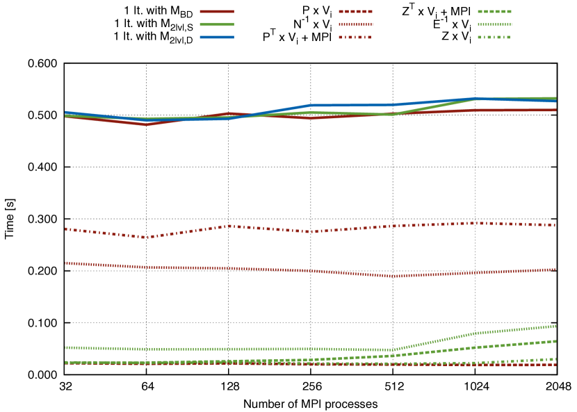
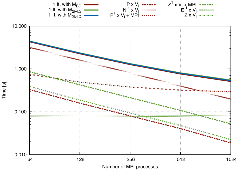
The total time breakdown between the main steps of one iteration of the preconditioned system is shown in Figure 10. The $60\%$ of the overall time is spent in the depointing operation, $\mathbf{P}^{t}_{j}\@vec{x}_{j}$, which requires communication, which is implemented in our code using a single global MPI_Allreduce. The second most expensive operation is the multiplication of the Toeplitz matrices by a vector, which is implemented with help of a parallel (multithreaded) FFT algorithm. Finally solving the small factorized linear system to compute $\mathbf{E}^{-1}\@vec{v}$ has an almost negligible impact on the total time but becomes progressively more important for the large test cases. However, the computations overall in the range of considered problem sizes scale well with the growing number of processors. Moreover, the time per iteration of the CG solver preconditioned by our two level preconditioner is almost the same as the time per iteration of the CG that is preconditioned by the standard preconditioner, as the solid red, green, and blue lines in Figure 10 nearly overlap. This also explains the good performance of our preconditioner, which requires a smaller number of iterations and, hence, a smaller overall time to solution.

In summary, our current implementation of the map-making software makes a convincing case for the superior overall efficiency of the new preconditioners proposed and studied in this work. Though additional optimisations can be implemented, as, for instance, included in the MADmap code (Cantalupo et al. 2010), these are not expected to change our conclusions in any major way as they are largely derived from comparisons of the relative performance as the major optimisations would affect the performance of both preconditioners to a similar extent. Consequently, as long as the cost of solving the system with the factorized matrix $\mathbf{E}$ and operations with $\mathbf{Z}$ remain subdominant with respect to the remaining steps of algorithm, the speedup factors measured in our experiments should be recovered.

Appendix D Role and impact of the assumed noise correlation length

Figure 11: Effects of imposing band-diagonality on the inverse noise correlation matrix, $\mathbf{N}^{-1}$, right panel, and its consequences for the inverse noise power spectrum, $P(f)$, left panel. The apodization kernel used here is defined in equation (32). The right panel shows a first row of the matrix, which is assumed to be Toeplitz. In both panels, solid lines show the result derived for the noise spectrum as in equation (21) without applying any apodization. Dashed lines show the results when the apodization is applied with the kernel length, $\lambda_{T}$, assuming values, $10^{4},2000,500$ and $100$, as shown bottom-up, in the left panel, and right-to-left in the right panel. Dash-dot-dash lines in the left panel show the characteristic frequency at which the apodized spectrum deflects from the original one for each apodization length. This frequency is given by $f_{defl}=1/\pi\lambda_{T}t_{samp}$.

In the presence of the off-diagonal correlations and assuming the noise correlation matrix that describes the piece-wise stationary noise present in the input time-ordered data, it is often convenient to think of the map-making problem in the Fourier rather than time domain. In this case, the data are represented as complex amplitudes of the Fourier modes as

$$\widetilde{\@vec{d}}:=\mathbf{F}\,\@vec{d},$$ (27)

where $\mathbf{F}$ is a block diagonal matrix with the blocks corresponding to the Fourier operators that acts independently on each stationary interval. Consequently, the sizes of the blocks reflect those of the inverse noise correlation matrix, $\mathbf{N}^{-1}$, in equation (4). Moreover, given the Toeplitz character of the blocks of the latter, we have

$$\widetilde{\mathbf{N}}^{-1} := \mathbf{F}^{T}\,\mathbf{N}^{-1}\,\mathbf{F}\simeq$$

$$\simeq \begin{pmatrix}{\displaystyle{\rm diag}\,P_{0}^{-1}\left(f\right)}&{\displaystyle 0}&{\displaystyle\dots}&{\displaystyle 0}\\ {\displaystyle 0}&{\displaystyle{\rm diag}\,P_{1}^{-1}\left(f\right)}&{\displaystyle\vdots}&{\displaystyle\vdots}\\ {\displaystyle\vdots}&{\displaystyle\dots}&{\displaystyle\ddots}&{\displaystyle 0}\\ {\displaystyle 0}&{\displaystyle\dots}&{\displaystyle\dots}&{\displaystyle{\rm diag}\,P_{K-1}^{-1}\left(f\right)}\end{pmatrix},$$

and therefore, the noise matrices in this representation are essentially diagonal with the diagonal given by an inverse noise power spectra for each of the stationary intervals. These can be typically parametrized as in equation (21).

The map-making process in the Fourier domain can be written as in equation (3),

$$\@vec{m}=\left[(\mathbf{F\,P})^{\,t}\,\widetilde{\mathbf{N}}^{-1}\,\mathbf{F\,P}\right)^{-1}\,\mathbf{F\,P}^{\,t}\,\mathbf{\widetilde{N}}^{-1}\,\widetilde{\@vec{d}},$$ (29)

and comes down to weighting of the Fourier amplitudes that represents the data. $\widetilde{\@vec{d}}$, by respective amplitudes of the noise power spectra, $P^{-1}_{j}(f)$. These are subsequently projected to the pixel domain by the projection operator, $(\mathbf{F\,P})^{\,t}$, and one corrected for by the weight matrix, $\left[(\mathbf{F\,P})^{\,t}\,\widetilde{\mathbf{N}}^{-1}\,\mathbf{F\,P}\right)^{-1}$. We note that this is analogous to what happens in the pixel domain if the time-domain noise is uncorrelated but potentially inhomogeneous. The first step of the map-making process is then a simple noise-weighted co-addition of the data in the pixels on the sky. We point out that the resulting map will still be unbiased, but potentially noisier than necessary in both cases, if our assumptions about the time- or frequency- domain weights are wrong.

For each Toeplitz block of the full inverse noise correlation matrix, the corresponding inverse noise power spectrum can be calculated by computing a Fourier transform of one of its rows. For the noise models in equation (21), these Toeplitz blocks are not generally band-diagonal. This is because the inverse power spectrum, as shown with a solid line in Figure 11, is never flat even at the lowest considered frequencies. If band-diagonality is desired, it would have to be therefore imposed. This corresponds to apodizing the row of the Toeplitz matrix with an appropriately chosen apodization window. The respective inverse noise power spectrum after the apodization is then given by a convolution of the Fourier transform of the window and the initial inverse power spectrum. In the time domain, the apodization window, which is required for this task, has to fall off quickly at some required correlation length, $\lambda_{T}$, which defines the effective bandwidth. Its Fourier representation also does so but at the scale given by $f_{defl}\equiv 1/(\pi\lambda_{T}\,t_{samp})$, where $t_{samp}$ stands for the sampling rate, as in equation (21). The convolution of this spectrum with the initial one therefore flattens the noise spectrum at the low frequency end with flattening that extends up to $f_{defl}$. This is illustrated in Figure 11, where we used a Gaussian window for the apodization,

$${\cal G}(k)=\left\{\begin{array}[]{l l}\vskip 6.0pt plus 2.0pt minus 2.0pt{\displaystyle\exp 2\,\left(\frac{k}{\lambda_{T}}\right)^{2},}&{\displaystyle k\leq\lambda_{T};}\\ {\displaystyle 0,}&{\displaystyle{\rm otherwise.}}\end{array}\right.$$ (32)

Consequently, imposing the band-diagonality modifiies the inverse noise power spectra and, therefore, weights, which are used in the map-making process, and, therefore, generally leads to suboptimal maps. How big is the loss and, in particular, whether it is acceptable, depends on how the sky signal is distributed in the Fourier domain. If the sky signal resides only in the frequency above some threshold, $\lower 2.15277pt\hbox{$\;\buildrel>\over{\sim}\;$}f_{sig}$, there is no loss of precision as long as $f_{sig}\lower 2.15277pt\hbox{$\;\buildrel>\over{\sim}\;$}f_{defl}$ and, therefore, as long as $\lambda_{T}\lower 2.15277pt\hbox{$\;\buildrel>\over{\sim}\;$}1/(\pi f_{sig}\,t_{samp})$. In practice, such circumstances are realised only for some periodic scanning strategies (e.g., Stompor & White 2004) and, more commonly, at least some part of the sky signal is present at arbitrary low, though non-zero, frequencies. In such cases, the magnitude of the precision loss clearly depends on the properties of the low frequency noise, such as its knee frequency and slope with the effect becoming larger for larger values of $f_{knee}$ and steeper noise spectra. For given noise properties and a scan strategy, if the loss is found unacceptably large, it can be mitigated by appropriately increasing the bandwidth width, as is indeed the standard rule of thumb used in the map-making community. However, the extra amount of the bandwidth, which is needed to ensure some required precision, depends on the sky signal distribution in the frequency domain.

We also note that $1/(\pi t_{samp}f_{knee})$ defines a maximal bandwidth, which is still merely equivalent to uniform weighting in the frequency domain and white noise weighting in the time domain. Therefore, only by adopting a larger bandwidth, we can obtain any improvement over the map produced with white noise weighting that is when all Toeplitz blocks are assumed proportional to unity.

The purpose of extending the correlation length is not so much to help to include the constraints coming from the very low frequency modes on the sky signal, as these are very noisy to start with and therefore, can anyway provide only weak constraints, but to ensure that those modes are properly weighted down, so the noise they contain does not overwhelm the constraints from higher frequencies where the noise per frequency is lower. Though filtering out these modes by setting the corresponding inverse power spectrum weights to zero, could avoid this issue, this procedure has to be consistently included in the calculation of the weight matrix, $(\mathbf{P}^{\,t}\mathbf{N}^{-1}\mathbf{P})^{-1}$, if an unbiased map estimate is to be derived. This, in turn, entails an effective increase of the actual bandwidth of the inverse noise correlation matrix, $\mathbf{N}^{-1}$, and typically enhances the level of noise correlations of the produced map. The trade-off in this case is therefore among the magnitude of the bias, the noise matrix bandwidth, and the complexity of the pixel-domain noise.

If the actual noise spectrum is more complex, and in particular, if it has some narrow features, then these also are affected as a result of imposing the band-diagonality.

References

- Armitage & Wandelt (2004) Armitage, C. & Wandelt, B. D. 2004, Phys. Rev. D, 70, 123007
- Bjorck (1996) Bjorck, A. 1996, Numerical Methods for Least Squares Problems, Handbook of Numerical Analysis (Society for Industrial and Applied Mathematics)
- Borrill (1999) Borrill, J. 1999, ArXiv Astrophysics e-prints
- Cantalupo et al. (2010) Cantalupo, C. M., Borrill, J. D., Jaffe, A. H., Kisner, T. S., & Stompor, R. 2010, The Astrophys. Journal Suppl. Series, 187, 212
- Cargemel et al. (2013) Cargemel, P., Grigori, L., & Stompor, R. 2013, submitted to Parallel Computing
- Challinor & Lewis (2011) Challinor, A. & Lewis, A. 2011, Phys.Rev., D84, 043516
- Chapman & Saad (1996) Chapman, A. & Saad, Y. 1996, Numer. Linear Algebra Appl, 4, 43
- de Bernardis et al. (2000) de Bernardis, P., Ade, P. A. R., Bock, J. J., et al. 2000, Nature, 404, 955
- de Gasperis et al. (2005) de Gasperis, G., Balbi, A., Cabella, P., Natoli, P., & Vittorio, N. 2005, Astronomy and Astrophysics, 436, 1159
- De Gersem & Hameyer (2001) De Gersem, H. & Hameyer, K. 2001, The European Physical Journal Applied Physics, 13, 45
- Doré et al. (2001) Doré, O., Teyssier, R., Bouchet, F. R., Vibert, D., & Prunet, S. 2001, A&A, 374, 358
- Erhel & Guyomarc’h (1997) Erhel, J. & Guyomarc’h, F. 1997, An Augmented Subspace Conjugate Gradient, Rapport de recherche RR-3278, INRIA
- Erhel & Guyomarc’h (2000) Erhel, J. & Guyomarc’h, F. 2000, SIAM J. Matrix Anal. Appl., 21, 1279
- Golub & Van Loan (1996) Golub, G. & Van Loan, C. 1996, Matrix computations, Vol. 3 (Johns Hopkins Univ Pr)
- Górski et al. (2005) Górski, K. M., Hivon, E., Banday, A. J., et al. 2005, The Astrophysical Journal, 622, 759
- Gosselet & Rey (2003) Gosselet, P. & Rey, C. 2003, in Domain decomposition methods in science and engineering (Natl. Auton. Univ. Mex., México), 419–426 (electronic)
- Grigori et al. (2012) Grigori, L., Stompor, R., & Szydlarski, M. 2012, in Proceedings of the International Conference on High Performance Computing, Networking, Storage and Analysis, SC ’12 (Los Alamitos, CA, USA: IEEE Computer Society Press), 91:1–91:10
- Gutknecht (2012) Gutknecht, M. 2012, Electron.Trans. Numer. Anal., 39, 156
- Hanany et al. (2000) Hanany, S., Ade, P., Balbi, A., et al. 2000, ApJ, 545, L5
- Harrison et al. (2011) Harrison, D. L., van Leeuwen, F., & Ashdown, M. A. J. 2011, A&A, 532, A55
- Havé et al. (2013) Havé, P., Masson, R., Nataf, F., et al. 2013, SIAM Journal on Scientific Computing, 35, C284
- Hestenes & Stiefel (1952) Hestenes, M. R. & Stiefel, E. 1952, Journal of Research of the National Bureau of Standards, 49, 409
- Keihänen & Reinecke (2012) Keihänen, E. & Reinecke, M. 2012, A&A, 548, A110
- Kharchenko & Yeremin (1995) Kharchenko, S. A. & Yeremin, A. Y. 1995, Numer. Linear Algebra Appl., 2, 51
- Morgan (1995) Morgan, R. 1995, SIAM Journal on Matrix Analysis and Applications, 16, 1154
- Næss & Louis (2013) Næss, S. & Louis, T. 2013, ArXiv e-prints
- Nicolaides (1987) Nicolaides, R. A. 1987, SIAM Journal on Numerical Analysis, 24, 355
- Oh et al. (1999) Oh, S. P., Spergel, D. N., & Hinshaw, G. 1999, ApJ, 510, 551
- Parks et al. (2006) Parks, M. L., de Sturler, E., Mackey, G., Johnson, D. D., & Maiti, S. 2006, SIAM J. Sci. Comput., 28, 1651
- Patanchon et al. (2008) Patanchon, G., Ade, P. A. R., Bock, J. J., et al. 2008, Astrophysical Journal, 681, 708
- Planck Collaboration et al. (2013) Planck Collaboration, Ade, P. A. R., Aghanim, N., Armitage-Caplan, C., & et al. 2013, ArXiv e-prints
- Risler & Rey (2000) Risler, F. & Rey, C. 2000, Numer. Algorithms, 23, 1
- Saad (2003) Saad, Y. 2003, Iterative Methods for Sparse Linear Systems: Second Edition (Society for Industrial and Applied Mathematics)
- Saad & Schultz (1986) Saad, Y. & Schultz, M. H. 1986, SIAM J. Sci. Stat. Comput., 7
- Saad et al. (2000) Saad, Y., Yeung, M., Erhel, J., & Guyomarc’h, F. 2000, SIAM J. Sci. Comput., 21, 1909, iterative methods for solving systems of algebraic equations (Copper Mountain, CO, 1998)
- Stompor et al. (2002) Stompor, R., Balbi, A., Borrill, J. D., et al. 2002, Phys. Rev. D, 65, 022003
- Stompor & White (2004) Stompor, R. & White, M. 2004, A&A, 419, 783
- Sudarsan et al. (2011) Sudarsan, R., Borrill, J., Cantalupo, C., et al. 2011, in Proceedings of the international conference on Supercomputing, ICS ’11 (New York, NY, USA: ACM), 305–316
- Sutton et al. (2009) Sutton, D., Johnson, B. R., Brown, M. L., et al. 2009, Monthly Notices of the Royal Astronomical Society, 393, 894
- Tang et al. (2009) Tang, J. M., Nabben, R., Vuik, C., & Erlangga, Y. A. 2009, J. Sci. Comput., 39, 340
- Tegmark (1997) Tegmark, M. 1997, Phys. Rev. D, 56, 4514
- Tegmark (1997) Tegmark, M. 1997, The Astrophysical Journal Letters, 480, L87
- van der Sluis & van der Vorst (1986) van der Sluis, A. & van der Vorst, H. A. 1986, Numerische Mathematik, 48, 543
- Vuik et al. (2006) Vuik, C., Nabben, R., & Tang, J. 2006, in Proceedings of the 8th European Multigrid Conference September 27-30, 2005 Scheveningen The Hague, The Netherlands, ed. P. Wesseling, C. Oosterlee, & P. Hemker (Delft: TU Delft)
- Wandelt & Hansen (2003) Wandelt, B. D. & Hansen, F. K. 2003, Phys. Rev. D, 67, 023001
- Wright et al. (1996) Wright, E. L., Hinshaw, G., & Bennett, C. L. 1996, The Astrophysical Journal Letters, 458, L53