Renormalization of a one-parameter family of piecewise isometries

J. H. Lowenstein and F. Vivaldi
( Dept. of Physics, New York University, 2 Washington Place, New York, NY 10003, USA
†School of Mathematical Sciences, Queen Mary, University of London, London E1 4NS, UK
)
Abstract

We consider a one-parameter family of piecewise isometries of a rhombus. The rotational component is fixed, and its coefficients belong to the quadratic number field K=(2)𝐾2K=\mathbb{Q}(\sqrt{2}). The translations depend on a parameter s𝑠s which is allowed to vary in an interval. We investigate renormalizability. We show that recursive constructions of first-return maps on a suitable sub-domain eventually produce a scaled-down replica of this domain, but with a renormalized parameter r(s)𝑟𝑠r(s). The renormalization map r𝑟r is the second iterate of a map f𝑓f of the generalised Lüroth type (a piecewise-affine version of Gauss’ map). We show that exact self-similarity corresponds to the eventually periodic points of f𝑓f, and that such parameter values are precisely the elements of the field K𝐾K that lie in the given interval.

The renormalization process is organized by a graph analogous to those used to construct renormalizable interval-exchange transformations. There are ten distinct renormalization scenarios corresponding to as many closed circuits in the graph. The process of induction along some of these circuits involves intermediate maps undergoing, as the parameter varies, infinitely many bifurcations.

Our proofs rely on computer-assistance.

1 Introduction

In piecewise isometries (PWI), renormalizability is a key for a complete description of the dynamics. The phase space of these systems is partitioned into domains, called atoms, over each of which the dynamics is an isometry. By choosing a sub-domain of the original space —typically an atom or a union of atoms— and considering the first-return map to it, one constructs a new system, the induced PWI on the chosen domain. If this process is repeated, then it may happen that an induced system be conjugate to the original system. This circumstance usually leads to a detailed understanding of the dynamics.

In one-dimension (interval-exchange transformations —IET) there is a satisfactory theory of renormalization. The Rauzy induction gives a criterion for selecting an interval (not one of the atoms) over which to induce, resulting in a new IET with the same number of atoms [19, 22]. This induction process is a dynamical system over a finite-dimensional space of IETs, related to the continued fractions algorithm, which affords a good description of the parameter space of IETs [23].

An important connection with Diophantine arithmetic is provided by the Boshernitzan and Carrol theorem [4]; it states that in any IET defined over a quadratic number field, inducing on any of the atoms results in only finitely many distinct IETs, up to scaling. For a two-interval exchange, this finiteness result reduces to Lagrange’s theorem on the eventual periodicity of the continued fractions expansions of quadratic surds. Furthermore, if a (uniquely ergodic) IET is renormalizable, then the scaling constant involved in renormalization is a unit in a distinguished ring of algebraic integers [18].
Refer to caption
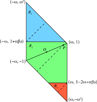
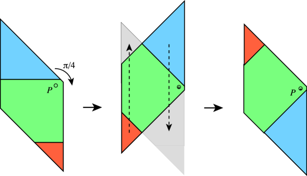
Figure 1: Our model: a rhombus RR\mathrm{R} with vertex angle π/4𝜋4\pi/4 is rotated clockwise by π/4𝜋4\pi/4 about a parameter-dependent fixed point P𝑃P located on the short diagonal. This leaves two triangular pieces outside the boundary of RR\mathrm{R}. These are translated vertically back into RR\mathrm{R} to complete the piecewise isometry.

In two dimensions general results are scarce [16, 17]. Until recently detailed results on renormalization were limited to special cases, defined over quadratic number fields [13, 1, 11, 2, 20]. These results point consistently towards the existence of a two-dimensional analogue of the B&C theorem. A more intricate form of renormalization has also been found in a handful of cubic cases [9, 14]. In all cases, the renormalization constants are units in the ring of integers of the field of definition of the PWI.

More recently, renormalization has been studied in parametrised families. Hooper considered a two-parameter family of rectangle exchange transformations, and used techniques connected to the renormalization of Truchet tilings to establish results on the measure of the periodic and aperiodic sets of the map [10]. In a substantial monograph [21], Schwartz determined the renormalization group of a one-parameter family of polygon-exchange transformations, where the exchange is achieved by translations only. In this model, inducing on suitable domains leads to a conjugacy of the map to its inverse, accompanied by a change of parameter given by a piecewise-Möbius map (a variant of Gauss’ map). Metric and topological properties of the limit set are also established.

In the present work we consider a family of PWIs of a rhombus RR\mathrm{R} with rotation angle π/4𝜋4-\pi/4 and a fixed point P𝑃P which is allowed to vary along the short diagonal, controlled by a real parameter s𝑠s (see figure 1). The choice of rotation determines the quadratic number field (2)2\mathbb{Q}(\sqrt{2}). Some special parameter values in this field (s=0,1+2,2(1+2))s=0,1+\sqrt{2},2(1+\sqrt{2})) have received much attention [1, 11, 2]; they correspond to P𝑃P being the centre and a vertex of the rhombus. These PWIs show exact self-similarity, and, as a result, their dynamics is well-understood.

For all maps in our family, the edges of the atoms have normal vectors in (2)2superscript22\mathbb{Q}(\sqrt{2})^{2}, while the Cartesian coordinates of the vertices belong to (2)+(2)s22𝑠\mathbb{Q}(\sqrt{2})+\mathbb{Q}(\sqrt{2})s, which is a two-dimensional vector space over (2)2\mathbb{Q}(\sqrt{2}). The same is true of the first-return map induced on any of the atoms, and recursively, of any higher-level induced return maps. This arithmetical environment will have a profound effect on the renormalization.

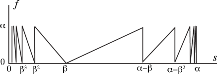
We have two main results, theorems 1 and 2, stated in section 4. In theorem 1 we prove that the parametrised rhombus map, restricted to the parameter interval sI=[0,2]𝑠𝐼02s\in I=[0,\sqrt{2}], induces in one of its triangular atoms a renormalizable five-atom PWI, i.e., one which, after repeated inductions, recurs at smaller length scales with a piecewise-affine change of parameter sr(s)maps-to𝑠𝑟𝑠s\mapsto r(s). We show that r𝑟r is the second iterate of a modified Lüroth map f𝑓f (a piecewise affine version of the Gauss map for continued fractions), which is shown in figure 2. We also show that all scaling constants are units in the ring [2]delimited-[]2\mathbb{Z}[\sqrt{2}].

Exact self-similarity is achieved if the induction process eventually reproduces a value of s𝑠s which has already been encountered, i.e., if s𝑠s is an eventually periodic point of r𝑟r. In theorem 2 we prove that these parameter values are precisely the elements of (2)I2𝐼\mathbb{Q}(\sqrt{2})\cap I. Note that, unlike the classic case of continued fractions, here eventual periodicity is associated with a single quadratic field. This arithmetical characterisation of renormalizability provides additional evidence for the existence of an analogue of the B&C theorem for polygon-exchange transformations.
Refer to caption
Figure 2: The piecewise-affine renormalization function f𝑓f which controls the renormalization of the piecewise isometry ρ=ρ(s)𝜌𝜌𝑠\rho=\rho(s) defined in section 3. Here α=2𝛼2\alpha=\sqrt{2}, β=α1𝛽𝛼1\beta=\alpha-1, and the function f𝑓f maps the parametric interval I=[0,α)𝐼0𝛼I=[0,\alpha) into itself.

The discontinuities of the function r𝑟r accumulate at the infinitely many zeros of f𝑓f (see figure 7). As a result, the return-map dynamics is highly non-uniform, with ever-increasing return times as s𝑠s approaches such discontinuities. The number of qualitatively distinct renormalization scenarios can be reduced to ten. The simplest of these involves a single induction, and it applies to the case in which both s𝑠s and f(s)𝑓𝑠f(s) are in the middle of the interval I𝐼I .

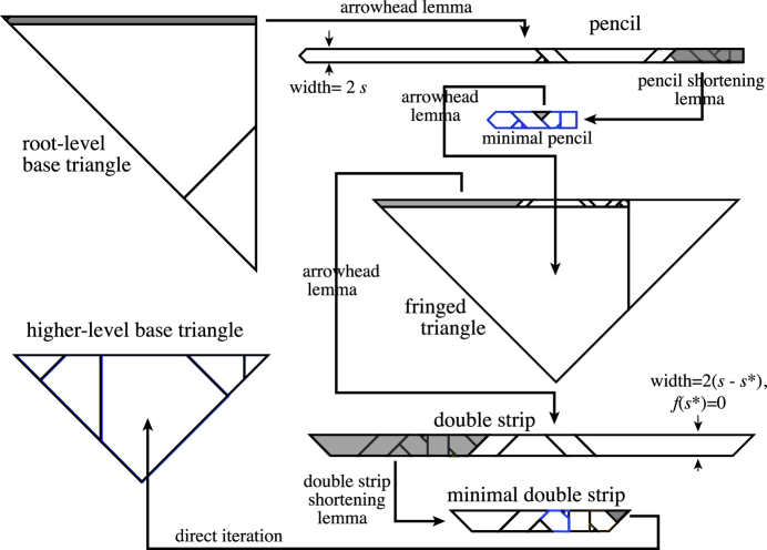
At the opposite extreme are, among others, those parts of I𝐼I for which both s𝑠s and 2f(s)2𝑓𝑠\sqrt{2}-f(s) are small. As a preview of renormalization dynamics, let us briefly sketch this scenario, represented schematically in figure 3. In this scheme, the number of inductions remains fixed at six, and it involves the same types of induced PWIs (the pencil, the fringed triangle, and the double strip). For either s𝑠s or f(s)𝑓𝑠f(s) approaching zero or 22\sqrt{2}, the numbers of atoms increases without bounds, but in a tightly controlled manner (the complexity increases logarithmically). The return times are are also unbounded.
Refer to caption
Figure 3: Sketch of the renormalization scenario for s𝑠s close to 0 and f(s)𝑓𝑠f(s) close to 22\sqrt{2}. In the figure, the relative sizes of the various objects are greatly distorted in order to reveal their structure.

The map f𝑓f serves as a phase function for the evolution of the pencil with decreasing s𝑠s, with two new atoms emerging at the boundary whenever f(s)𝑓𝑠f(s) passes through unity. Analogously, bifurcations of the double strip occur at the zeros of r(s)𝑟𝑠r(s). The spatial scaling accompanying the renormalization is governed by the successive narrowing of the widths of the pencil and the double strip.

Of the six induction steps, two are ‘shortenings’, exploiting the repetitive, quasi-one-dimensional structures of pencils and double strips. Steps 1, 3, and 4 appear to be more complicated, but in fact are all grounded in one simple dynamical sub-system, the arrowhead. Once we have formulated that underlying dynamics in the Arrowhead Lemma of section 9, all aforementioned induction steps can be split into two manageable parts: the first, with short, fixed-length return orbits which can be constructed by explicit iteration, and the second, in which the Arrowhead Lemma accounts for all of the s𝑠s-dependent bifurcations.

1.1 Structure of the paper

Sections 2–4: Preliminaries, and formulation of the main results

In section 2 we provide definitions and notation which will be used throughout, followed by the specification of our model in section 3. In section 4 we define the renormalization function f𝑓f and r𝑟r and state our two main theorems. The first of these, theorem 1, describes the renormalization of our central geometric structure, the two-parameter base triangle with its five-atom piecewise isometry. The second, theorem 2, introduces the symbolic dynamics of the renormalization and establishes the connection between exact self-similarity and membership in the field (2)2\mathbb{Q}(\sqrt{2}).

Sections 5,6: Symbolic dynamics, Lüroth expansion, proof of theorem 2

After introducing a symbolic representation of parameter space in section 5, we derive the Lüroth expansion and prove theorem 2 using a contraction argument on a lattice.

Section 7: Renormalization overview

Here we provide roadmaps for navigating the rest of the paper, organized around a renormalization graph, analogous to the Rauzy graphs of interval exchange theory [19]. Oriented edges of the graph correspond to various return-map inductions, and closed circuits describe the ten distinct pathways by which one succeeds in renormalizing the initial base triangle on various subsets of the parameter interval I𝐼I.

Sections 8,9: Machinery for proving theorem 1

In section 8 we define the parametric dressed domains (tiled polygons with associated piecewise isometries) which correspond to the vertices of the renormalization graph: the pencil, the fringed triangle, and the double strip. In addition, we prove two Shortening Lemmas which allow one to reduce pencils and double strips to their minimum lengths. Section 9 is devoted to the arrowhead and its dynamics, culminating in the Arrowhead Lemma.

Section 10: Proof of theorem 1

Through a sequence of propositions, we treat all of the various induction steps needed to prove theorem 1 over the entire interval I𝐼I. Some of the induction steps require only explicit iteration of PWIs over short orbits of fixed length, while others require, in addition, application of one of the Shortening Lemmas or the Arrowhead Lemma.

Section 11: Temporal scaling and fractal structure

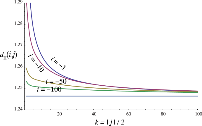
As a by-product of section 10, we obtain the incidence matrices which determine the renormalization’s return times and asymptotic temporal scaling. We obtain explicit formulae for these matrices in section 11, where we also explore briefly the implications for the s𝑠s-dependence of the Hausdorff dimension of the exceptional set.

Many steps in the proofs have required computer assistance, invariably to verify statements concerning finite orbits of PWIs. This requires geometrical transformations of polygons (translations, rotations, reflections, etc.), polygon inclusion and disjointness tests, plus a fair amount of book-keeping. All arithmetic is performed exactly in (2)2\mathbb{Q}(\sqrt{2}) and (2)+(2)s22𝑠\mathbb{Q}(\sqrt{2})+\mathbb{Q}(\sqrt{2})s. The complexity of the computation is manageable, because all of the heavy lifting is taken care by the Arrowhead and Shortening lemmas, which are proved analytically. A complete description and listing of our procedures, in the form of Mathematica®functions, together with all of the calculations participating in the proof of theorem 1, may be found in the Electronic Supplement [6].


Acknowledgements: JHL and FV would like to thank, respectively, the School of Mathematical Sciences at Queen Mary, University of London, and the Department of Physics of New York University, for their hospitality.

2 Definitions and notation

Throughout this article we adopt the notation

α=2,β=21,ω=2+1.formulae-sequence𝛼2formulae-sequence𝛽21𝜔21\alpha=\sqrt{2},\quad\beta=\sqrt{2}-1,\quad\omega=\sqrt{2}+1.

The arithmetical environment is the algebraic number field (α)𝛼\mathbb{Q}(\alpha) with its ring of integers [α]delimited-[]𝛼\mathbb{Z}[\alpha], given by

(α)={x+yα:x,y},(α)={m+nα:m,n}.formulae-sequence𝛼conditional-set𝑥𝑦𝛼𝑥𝑦𝛼conditional-set𝑚𝑛𝛼𝑚𝑛\mathbb{Q}(\alpha)=\{x+y\alpha\,:\,x,y\in\mathbb{Q}\},\qquad\mathbb{Z}(\alpha)=\{m+n\alpha\,:\,m,n\in\mathbb{Z}\}. (1)

The number ω𝜔\omega, which will be shown to determine the scaling, is the fundamental unit in [α]delimited-[]𝛼\mathbb{Z}[\alpha] (see [5, chapter 6]). Note that β=ω1𝛽superscript𝜔1\beta=\omega^{-1} is also a unit.

Our system depends on a parameter s𝑠s, and to represent parameter dependence we consider the set

𝕊=(α)+(α)s𝕊𝛼𝛼𝑠{\mathbb{S}}=\mathbb{Q}(\alpha)+\mathbb{Q}(\alpha)s (2)

Here, and below, s𝑠s is regarded as an indeterminate; hence the set 𝕊𝕊{\mathbb{S}} is a two-dimensional vector space over (α)𝛼\mathbb{Q}(\alpha) (a (α)𝛼\mathbb{Q}(\alpha)-module) whose elements are degree-one polynomials in s𝑠s.

2.1 Planar objects

A tile is an open convex polygon whose edges have outward normal vectors taken from the set {𝐮m=(cosmπ/4,sinmπ/4):m=0,,7}conditional-setsubscript𝐮𝑚𝑚𝜋4𝑚𝜋4𝑚07\{\mathbf{u}_{m}=(\cos{m\pi/4},\sin{m\pi/4}):m=0,\ldots,7\}. The equations of the edges of an n𝑛n-sided tile are thus of the form

𝐮mi(x,y)=bi,i=1,,n,formulae-sequencesubscript𝐮subscript𝑚𝑖𝑥𝑦subscript𝑏𝑖𝑖1𝑛\mathbf{u}_{m_{i}}\cdot(x,y)=b_{i},\quad i=1,\ldots,n,

where the ‘octagonal coordinates’ bisubscript𝑏𝑖b_{i} belong to 𝕊𝕊\mathbb{S}. The parameter s𝑠s allows for the continuous deformation of tiles.

We represent an n𝑛n-sided tile X𝑋X with edge orientations m1,,mnsubscript𝑚1subscript𝑚𝑛m_{1},\ldots,m_{n} and octagonal coordinates b1,,bnsubscript𝑏1subscript𝑏𝑛b_{1},\ldots,b_{n} with the bracket notation

X=[(m1,,mn),(b1,,bn)].𝑋subscript𝑚1subscript𝑚𝑛subscript𝑏1subscript𝑏𝑛X=[(m_{1},\ldots,m_{n}),(b_{1},\ldots,b_{n})]. (3)

Tile names will always be capital italic letters.

A domain is a union of open polygons whose edges are specified by octagonal orientations 𝐮msubscript𝐮𝑚\mathbf{u}_{m} and coordinates in the module 𝕊𝕊\mathbb{S}. The polygons need not be convex. Domain names will always be capital Roman letters.

A tiling 𝐗𝐗{\bf X} is a set of tiles,

𝐗={X1,,Xn}.𝐗subscript𝑋1subscript𝑋𝑛{\bf X}=\{X_{1},\ldots,X_{n}\}.

A tiling 𝐗𝐗{\bf X} is always associated with a domain XX{\rm X}, the span of 𝐗𝐗{\bf X} ,

X=span(𝐗)=defInt(i=1nXi¯).Xspan𝐗superscriptdefInt¯superscriptsubscript𝑖1𝑛subscript𝑋𝑖{\rm X}={\rm span}({\bf X})\stackrel{{\scriptstyle\rm def}}{{=}}{\rm Int}(\overline{\cup_{i=1}^{n}X_{i}}).

The union of two tilings is a tiling.

2.2 Isometry group

We employ a group 𝔊𝔊\mathfrak{G} of transformations of planar objects, to specify their locations and orientations, and to describe their dynamical evolution. The group comprises the rotations and reflections of the symmetry group of the regular octagon (the dihedral group D8subscript𝐷8D_{8}) together with translations in 𝕊2superscript𝕊2\mathbb{S}^{2}. We define 𝔊+subscript𝔊\mathfrak{G}_{+} to be the subgroup of orientation-preserving transformations in 𝔊𝔊\mathfrak{G}, i.e., those with Jacobian determinant equal to +11+1.

We adopt the following notation:

  • 𝚄nsubscript𝚄𝑛\mathtt{U}_{n}: reflection about the lines generated by the extended set of vectors

    𝐮k=(cos(kπ/4),sin(kπ/4)),k=0,12,1,32,,formulae-sequencesubscript𝐮𝑘𝑘𝜋4𝑘𝜋4𝑘012132\mathbf{u}_{k}=(\cos(k\pi/4),\sin(k\pi/4)),\quad k=0,\frac{1}{2},1,\frac{3}{2},\ldots,

    where we allow for half-integer indices, to be taken modulo 8;

  • 𝚁nsubscript𝚁𝑛\mathtt{R}_{n}: rotation by the angle nπ/4,n=0,,7formulae-sequence𝑛𝜋4𝑛07n\pi/4,\;n=0,\ldots,7;

  • 𝚃𝐝subscript𝚃𝐝\mathtt{T}_{\bf d}: translation by 𝐝𝕊2𝐝superscript𝕊2{\bf d}\in\mathbb{S}^{2}.

Thanks to the product formulae

𝚃𝐝𝚃𝐞=𝚃𝐝+𝐞,𝚁m𝚁n=𝚁m+n,𝚄m𝚄n=𝚁2(mn),formulae-sequencesubscript𝚃𝐝subscript𝚃𝐞subscript𝚃𝐝𝐞formulae-sequencesubscript𝚁𝑚subscript𝚁𝑛subscript𝚁𝑚𝑛subscript𝚄𝑚subscript𝚄𝑛subscript𝚁2𝑚𝑛\mathtt{T}_{\bf d}\mathtt{T}_{\bf e}=\mathtt{T}_{{\bf d}+{\bf e}},\qquad\mathtt{R}_{m}\mathtt{R}_{n}=\mathtt{R}_{m+n},\qquad\mathtt{U}_{m}\mathtt{U}_{n}=\mathtt{R}_{2(m-n)},

and commutation relations

𝚁n𝚃𝐝=𝚃𝚁n𝐝𝚁n,𝚁n𝚄m=𝚄m+n𝚁n,𝚄n𝚃𝐝=𝚃𝚄n𝐝𝚄n,formulae-sequencesubscript𝚁𝑛subscript𝚃𝐝subscript𝚃subscript𝚁𝑛𝐝subscript𝚁𝑛formulae-sequencesubscript𝚁𝑛subscript𝚄𝑚subscript𝚄𝑚𝑛subscript𝚁𝑛subscript𝚄𝑛subscript𝚃𝐝subscript𝚃subscript𝚄𝑛𝐝subscript𝚄𝑛\mathtt{R}_{n}\mathtt{T}_{\bf d}=\mathtt{T}_{\mathtt{R}_{n}{\bf d}}\mathtt{R}_{n},\qquad\mathtt{R}_{n}\mathtt{U}_{m}=\mathtt{U}_{m+n}\mathtt{R}_{n},\qquad\mathtt{U}_{n}\mathtt{T}_{\bf d}=\mathtt{T}_{\mathtt{U}_{n}{\bf d}}\mathtt{U}_{n}, (4)

we can write an arbitrary element 𝙶𝙶\mathtt{G} of 𝔊𝔊{\mathfrak{G}} in the canonical form

𝙶n,m,𝐝=𝚃𝐝𝚁m𝚄0n,subscript𝙶𝑛𝑚𝐝subscript𝚃𝐝subscript𝚁𝑚subscriptsuperscript𝚄𝑛0\mathtt{G}_{n,m,{\bf d}}=\mathtt{T}_{\bf d}\mathtt{R}_{m}\mathtt{U}^{n}_{0},

with

n{0,1},m{0,1,,7},𝐝𝕊2.formulae-sequence𝑛01formulae-sequence𝑚017𝐝superscript𝕊2n\in\{0,1\},\quad m\in\{0,1,\ldots,7\},\quad\mathbf{d}\in\mathbb{S}^{2}.

In general, we will write 𝒳𝒴similar-to𝒳𝒴\mathcal{X}\sim\mathcal{Y} to indicate that 𝒳=𝙶(𝒴)𝒳𝙶𝒴\mathcal{X}=\mathtt{G}(\mathcal{Y}) for some 𝙶𝔊𝙶𝔊\mathtt{G}\in\mathfrak{G}. As 𝔊𝔊\mathfrak{G} is a group, this is an equivalence relation. An equivalence class consists of planar objects which are congruent (same shape and size) up to a reflection. Appendix A contains a catalogue of standard representatives of equivalence classes, used extensively in this work.

2.3 Dressed domains and subdomains

We define a dressed domain to be a triple

𝒳=(X,𝐗,ρ),𝒳X𝐗𝜌\mathcal{X}=({\mathrm{X},\mathbf{X},\rho}), (5)

where XX\mathrm{X} is a domain, 𝐗𝐗\mathbf{X} is a tiling with span XX\mathrm{X}, and ρ𝜌\rho is a mapping which acts on each element of 𝐗𝐗\mathbf{X} as an isometry in 𝔊+subscript𝔊\mathfrak{G}_{+}. We will describe ρ𝜌\rho as a piecewise isometry or domain map acting on XX\mathrm{X}, with 𝐗𝐗\mathbf{X} comprising the set of its atoms. Dressed domains will always be denoted by capital script letters. Under the action of an isometry 𝙶𝔊𝙶𝔊\mathtt{G}\in\mathfrak{G}, a dressed domain transforms as

𝙶(𝒳)=𝙶(X,𝐗,ρ)=(𝙶(X),{𝙶(X1),𝙶(X2),},𝙶ρ𝙶1).𝙶𝒳𝙶X𝐗𝜌𝙶X𝙶subscript𝑋1𝙶subscript𝑋2𝙶𝜌superscript𝙶1\mathtt{G}(\mathcal{X})=\mathtt{G}({\mathrm{X},\mathbf{X},\rho})=(\mathtt{G}(\mathrm{X}),\{\mathtt{G}(X_{1}),\mathtt{G}(X_{2}),\ldots\},\mathtt{G}\circ\rho\circ\mathtt{G}^{-1}).

To emphasize the association of a mapping ρ𝜌\rho with a particular dressed domain 𝒳𝒳\mathcal{X}, we will use the notation ρ𝒳subscript𝜌superscript𝒳absent\rho_{\stackrel{{\scriptstyle}}{{\mathcal{X}}}}.

Let 𝒳=(X,𝐗,ρ𝒳)𝒳X𝐗subscript𝜌superscript𝒳absent\mathcal{X}=(\mathrm{X},\mathbf{X},\rho_{\stackrel{{\scriptstyle}}{{\mathcal{X}}}}) be a dressed domain, and let YY\mathrm{Y} be a sub-domain of XX\mathrm{X}. We denote by ρ𝒴subscript𝜌superscript𝒴absent\rho_{\stackrel{{\scriptstyle}}{{\mathcal{Y}}}} the first-return map on YY\mathrm{Y} induced by ρ𝒳subscript𝜌superscript𝒳absent\rho_{\stackrel{{\scriptstyle}}{{\mathcal{X}}}}. We call the resulting dressed domain 𝒴=(Y,𝐘,ρ𝒴)𝒴Y𝐘subscript𝜌superscript𝒴absent\mathcal{Y}=(\mathrm{Y},\mathbf{Y},\rho_{\stackrel{{\scriptstyle}}{{\mathcal{Y}}}}) a dressed subdomain of 𝒳𝒳\mathcal{X}, writing

𝒳𝒴.𝒳𝒴\mathcal{X}\rightarrow\mathcal{Y}. (6)

A prototype is a canonical representative of an equivalence class of dressed domains. If 𝒳^^𝒳\widehat{\mathcal{X}} is a prototype and 𝒴𝒳^similar-to𝒴^𝒳\mathcal{Y}\sim\widehat{\mathcal{X}}, then the parity π(𝒴)𝜋𝒴\pi(\mathcal{Y}) of 𝒴𝒴\mathcal{Y} is the Jacobian determinant of the isometry in 𝔊𝔊\mathfrak{G} relating 𝒳^^𝒳\widehat{\mathcal{X}} to 𝒴𝒴\mathcal{Y}.

The dressed subdomain relation (6) enjoys the important property of scale invariance, namely invariance under an homothety. Indeed if 𝚂ωsubscript𝚂𝜔\mathtt{S}_{\omega} denotes scaling by a factor ω𝜔\omega, then in the data (3) specifying a tile, the orientations mksubscript𝑚𝑘m_{k} remain unchanged, while the octagonal coordinates bksubscript𝑏𝑘b_{k} scale by ω𝜔\omega. Moreover, the identity

𝚂ω𝚃𝐝𝚁n=𝚃ω𝐝𝚁n𝚂ω.subscript𝚂𝜔subscript𝚃𝐝subscript𝚁𝑛subscript𝚃𝜔𝐝subscript𝚁𝑛subscript𝚂𝜔\mathtt{S}_{\omega}\mathtt{T}_{\mathbf{d}}\mathtt{R}_{n}=\mathtt{T}_{\omega\mathbf{d}}\mathtt{R}_{n}\mathtt{S}_{\omega}.

shows that the piecewise isometries ρ𝜌\rho scale in the same way. We conclude that the relation (6) is preserved if the dressed domain parameters are scaled by the same factor for both members.

We shall be dealing with renormalizability of dressed domains depending on a parameter s𝑠s —the parametric dressed domains. The parameter s𝑠s, ranging over an interval I𝐼I, controls the ‘shape’ of the domain. For reasons that will become clear below, it is useful to re-parametrise the system with a pair (l,h)𝑙(l,h) where l𝑙l is a ‘size’ parameter ranging over the positive real numbers, and h=sl𝑠𝑙h=sl. So we shall write 𝒳=𝒳(l,h)𝒳𝒳𝑙\mathcal{X}=\mathcal{X}(l,h). Note that a parametric dressed domain need not have a fixed number of atoms. Indeed many of the parametric dressed domains introduced in section 8 feature an infinite sequence of bifurcations, each producing a change in the number and shapes of its atoms.

2.4 Renormalizability of dressed domains

A dressed domain 𝒳=(X,𝐗,ρ𝒳)𝒳X𝐗subscript𝜌superscript𝒳absent\mathcal{X}=({\mathrm{X},\mathbf{X},\rho_{\stackrel{{\scriptstyle}}{{\mathcal{X}}}}}) is strictly renormalizable if i)i) there exists a dressed subdomain 𝒴𝒴\mathcal{Y} of 𝒳𝒳\mathcal{X} and a dressed subdomain 𝒴superscript𝒴\mathcal{Y}^{*} of 𝒴𝒴\mathcal{Y}, which differs from 𝒴𝒴\mathcal{Y} by a contracting scale transformation (homothety) composed with an isometry from 𝔊𝔊\mathfrak{G}; ii)ii) the domain XX\mathrm{X} has the recursive tiling property, namely it is completely tiled (ignoring sets of zero measure) by the return orbits of the atoms of 𝒴superscript𝒴\mathcal{Y}^{*}, together with the periodic orbits of a finite set of tiles.

This is the simplest version of renormalizability. Its implications for a planar piecewise isometry are well-known (see, for example, [17], [12, chapter 2]). Thus one can iterate the process at will, and with each iteration more and more periodic domains of finer and finer scales are revealed, leading to a full measure of periodic tiles in the limit. Simultaneously, the return orbits of the rescaled copies of 𝒴𝒴\mathcal{Y}, provide finer and finer coverings of the exceptional set complementary to all periodic tiles. While the latter has vanishing measure, its dimension is not trivial. Standard arguments [7, 12] show that the Hausdorff dimension of the exceptional set is given by dH=logτ/logωsubscript𝑑𝐻𝜏𝜔d_{H}=-\log\tau/\log\omega, where ω𝜔\omega and τ𝜏\tau are, respectively the asymptotic spatial and temporal scale factors associated with the renormalization. The asymptotic spatial scaling is known, since each renormalization step is accompanied by multiplication by the same ω𝜔\omega. The temporal scaling is more subtle, requiring construction and diagonalization of the stepwise incidence matrix MM\mathrm{M}, whose i,j𝑖𝑗i,jth component gives —in the above notation— the number of times that the return orbit of atom Yjsubscriptsuperscript𝑌𝑗Y^{*}_{j} visits atom Yisubscript𝑌𝑖Y_{i}. The scale factor τ𝜏\tau governing the asymptotic increase in length of the return orbits is given by the largest eigenvalue of MM\mathrm{M}.

A parametric dressed domain 𝒴(l,h),l+,s=h/lIformulae-sequence𝒴𝑙𝑙subscript𝑠𝑙𝐼\mathcal{Y}(l,h),\;l\in\mathbb{R}_{+},\;s=h/l\in I, is said to be renormalizable if there exist a piecewise smooth renormalization map r:II:𝑟𝐼𝐼r:I\rightarrow I, and an auxiliary scaling function κ:+(0,1):𝜅subscript01\kappa:\mathbb{R}_{+}\rightarrow(0,1) such that for every choice of l𝑙l and hh, the dressed domain 𝒴(l,h)𝒴𝑙\mathcal{Y}(l,h) has a dressed subdomain congruent to 𝒴(l,h)𝒴superscript𝑙superscript\mathcal{Y}(l^{\prime},h^{\prime}) with (l,h)=(κ(s)l,r(s)κ(s)l)superscript𝑙superscript𝜅𝑠𝑙𝑟𝑠𝜅𝑠𝑙(l^{\prime},h^{\prime})=(\kappa(s)l,r(s)\kappa(s)l), and moreover the recursive tiling property is satisfied. In the present work, the renormalization map is piecewise-affine (as opposed to the piecewise-Möbius map of [21] and Gauss’ map) with derivative equal to 1/κ1𝜅1/\kappa. Furthermore, all values assumed by κ𝜅\kappa are units in the ring [2]delimited-[]2\mathbb{Z}[\sqrt{2}]. Note that r𝑟r and κ𝜅\kappa depend only on s𝑠s, a requirement of scale invariance. A parametric dressed domain which, for all valid parameter values, has a renormalizable parametric dressed sub-domain, with recursive tiling, will also be regarded as renormalizable.

If a parametric dressed domain 𝒴(l,h)𝒴𝑙\mathcal{Y}(l,h) is renormalizable, we can consider those parameter values for which 𝒴𝒴\mathcal{Y} is strictly renormalizable. Because of scale invariance, if 𝒴(l,h(l,s))𝒴𝑙𝑙𝑠\mathcal{Y}(l,h(l,s)) is strictly renormalizable for s=s0𝑠subscript𝑠0s=s_{0} and some l𝑙l, then it is so for any l𝑙l. It then follows that the s𝑠s-values of strict renormalizability are precisely the eventually periodic points of the function r𝑟r. A virtue of our model is an arithmetical characterization of these parameter values: they are precisely the elements of the quadratic number field (α)𝛼\mathbb{Q}(\alpha).

The above definition of renormalizability is tailored to our model and it is conceivable that in more general situations the recursive tiling property may require participation of more than one renormalizable parametric dressed sub-domain.

2.5 Computations

All computations reported in this work are exact, employing integer and polynomial arithmetic with Mathematica®. For fixed parameter value, the computations take place in the algebraic number field (α)𝛼\mathbb{Q}(\alpha) —see (1)— whereas the parametric dependence requires computations in the module 𝕊𝕊\mathbb{S} defined in (2).

All relevant objects are represented by data structures of elements of these two arithmetic sets. In particular, we shall be concerned with finite orbits of polygonal domains under the domain map of a dressed domain, which is an isometry in 𝔊𝔊\mathfrak{G}. To perform these computations we employ the procedures of our CAP Toolbox, available in the Electronic Supplement [6].

In such processes, one must determine membership of points to polygons and intersections of polygons, which requires the evaluation of inequalities. Since the latter are expressed by affine functions of s𝑠s, it suffices to check the inequalities at the endpoints of the assumed s𝑠s-interval. All these boundary values belong in the field (α)𝛼\mathbb{Q}(\alpha), and the inequalities are evaluated by estimating α=2𝛼2\alpha=\sqrt{2} via a pair of sufficiently close convergents in its continued fraction expansion. In this way we are able to establish statements valid over intervals of parameters.

Typically we are given a one-parameter family of piecewise isometries ρ(s)𝜌𝑠\rho(s) of a dressed domain (s)𝑠\mathcal{R}(s), which we use to move each tile in the domain from an initial position to a pre-assigned destination, checking at each step that no tile arrives at the wrong destination. Each iteration involves testing a number of half-plane inequalities to determine which atom Ri(s)subscript𝑅𝑖𝑠R_{i}(s) of ρ(s)𝜌𝑠\rho(s) contains a particular tile, followed by application of the relevant isometry ρi(s)subscript𝜌𝑖𝑠\rho_{i}(s) to map the tile forward. When constructing a finite orbit (typically a return orbit), we keep track of the atoms visited, obtaining at the end the symbolic paths and incidence matrices of the orbits. The recursive tiling property defined in section 2.4 is established by adding up the areas of the tiles of all the orbits, and comparing it with the total area of the parent domain.

Henceforth we will refer to this technique as direct iteration.

3 The model

We consider a one-parameter family ρ(s)𝜌𝑠\rho(s) of piecewise isometries on a fixed rhombus RR\mathrm{R} of side 2αω2𝛼𝜔2\alpha\omega and vertex angle π/4𝜋4\pi/4 (figure 4), specified by the half-plane conditions ui(x,y)<ω,i=0,1,4,5formulae-sequencesubscriptu𝑖𝑥𝑦𝜔𝑖0145\mathrm{u}_{i}\cdot(x,y)<\omega,\;i=0,1,4,5, i.e.,

R=[(0,1,4,5),(ω,ω,ω,ω)].R0145𝜔𝜔𝜔𝜔\mathrm{R}=[(0,1,4,5),(\omega,\omega,\omega,\omega)]. (7)

The map ρ(s)𝜌𝑠\rho(s) acts as an orientation-preserving isometry ρi(s)𝔊+subscript𝜌𝑖𝑠subscript𝔊\rho_{i}(s)\in\mathfrak{G}_{+} on each of its atoms: Ri,i=1,2,3formulae-sequencesubscript𝑅𝑖𝑖123R_{i},\;i=1,2,3,

R1(s)subscript𝑅1𝑠\displaystyle R_{1}(s) =\displaystyle= [(0,2,5),(ω,12α+αβs,ω)],025𝜔12𝛼𝛼𝛽𝑠𝜔\displaystyle[(0,2,5),(\omega,-1-2\alpha+\alpha\beta s,\omega)],
R2(s)subscript𝑅2𝑠\displaystyle R_{2}(s) =\displaystyle= [(0,1,2,4,5,6),(ω,ω,1+αβs,ω,ω,1+2ααβs)],012456𝜔𝜔1𝛼𝛽𝑠𝜔𝜔12𝛼𝛼𝛽𝑠\displaystyle[(0,1,2,4,5,6),(\omega,\omega,1+\alpha\beta s,\omega,\omega,1+2\alpha-\alpha\beta s)], (8)
R3(s)subscript𝑅3𝑠\displaystyle R_{3}(s) =\displaystyle= [(1,4,6),(ω,ω,1αβs)].146𝜔𝜔1𝛼𝛽𝑠\displaystyle[(1,4,6),(\omega,\omega,-1-\alpha\beta s)].

Specifically, each atomic isometry is a clockwise rotation by π/4𝜋4\pi/4 followed by an s𝑠s-dependent vertical translation,

ρ1(s)subscript𝜌1𝑠\displaystyle\rho_{1}(s) =\displaystyle= 𝚃(0,2β2βs)𝚁7,subscript𝚃02𝛽2𝛽𝑠subscript𝚁7\displaystyle\mathtt{T}_{(0,2\beta-2\beta s)}\mathtt{R}_{7},
ρ2(s)subscript𝜌2𝑠\displaystyle\rho_{2}(s) =\displaystyle= 𝚃(0,22βs)𝚁7,subscript𝚃022𝛽𝑠subscript𝚁7\displaystyle\mathtt{T}_{(0,-2-2\beta s)}\mathtt{R}_{7}, (9)
ρ3(s)subscript𝜌3𝑠\displaystyle\rho_{3}(s) =\displaystyle= 𝚃(0,2ω2βs)𝚁7.subscript𝚃02𝜔2𝛽𝑠subscript𝚁7\displaystyle\mathtt{T}_{(0,-2\omega-2\beta s)}\mathtt{R}_{7}.

For each value of s𝑠s in the interval [0,2ω]02𝜔[0,2\omega], the map ρ(s)𝜌𝑠\rho(s) has a fixed-point

P(s)=(ωs,1βs)𝑃𝑠𝜔𝑠1𝛽𝑠P(s)=(\omega-s,1-\beta s)

on the short diagonal of the rhombus. The renormalizability for the cases s=0,ω,2ω𝑠0𝜔2𝜔s=0,\omega,2\omega is known [1, 11, 2].

Refer to caption
Figure 4: Partition of the rhombus RR\mathrm{R} into atoms Ri,i=1,2,3formulae-sequencesubscript𝑅𝑖𝑖123R_{i},\;i=1,2,3. The piecewise isometry ρ(s)𝜌𝑠\rho(s) may be represented as a composition of two involutions: simultaneous reflection of the atoms about their respective symmetry axes (dashed lines), followed by reflection about the short diagonal of the rhombus (solid line). The intersection of these symmetry lines is a fixed point P𝑃P, located s𝑠s to the left and βs𝛽𝑠\beta s below the vertex (ω,1)𝜔1(\omega,1).

The piecewise isometry ρ(s)𝜌𝑠\rho(s) is reversible, namely it can be written as the composition of two orientation-reversing involutions,

ρ(s)=𝙶𝙷(s),𝙶2=𝙷(s)2=𝟏,formulae-sequence𝜌𝑠𝙶𝙷𝑠superscript𝙶2𝙷superscript𝑠21\rho(s)=\mathtt{G}\circ\mathtt{H}(s),\qquad\mathtt{G}^{2}=\mathtt{H}(s)^{2}={\bf 1},

where 𝙷(s)𝙷𝑠\mathtt{H}(s) is the simultaneous reflection of the three atoms about their respective symmetry axes, and 𝙶𝙶\mathtt{G} is the reflection of the rhombus RR\mathrm{R} about its short diagonal. Note that the fixed point P𝑃P is symmetric, namely it lies at the intersection of fixed lines of 𝙶𝙶\mathtt{G} and 𝙷𝙷\mathtt{H}. Moreover, 𝙷=𝙶ρ𝙷𝙶𝜌\mathtt{H}=\mathtt{G}\circ\rho, and either 𝙶𝙶\mathtt{G} or 𝙷𝙷\mathtt{H} serves as a time-reversal operator for the map ρ𝜌\rho:

𝙶ρ(s)𝙶=𝙷ρ(s)𝙷=ρ(s)1.𝙶𝜌𝑠𝙶𝙷𝜌𝑠𝙷𝜌superscript𝑠1\mathtt{G}\circ\rho(s)\circ\mathtt{G}=\mathtt{H}\circ\rho(s)\circ\mathtt{H}=\rho(s)^{-1}.

Another useful symmetry relation follows from the invariance of the rhombus under 𝚁4subscript𝚁4\mathtt{R}_{4} (rotation by π𝜋\pi), which takes (x,y)𝑥𝑦(x,y) into (x,y)𝑥𝑦(-x,-y). One readily verifies that

𝚁4ρ(s)𝚁4=ρ(2ωs).subscript𝚁4𝜌𝑠subscript𝚁4𝜌2𝜔𝑠\mathtt{R}_{4}\circ\rho(s)\circ\mathtt{R}_{4}=\rho(2\omega-s).

In studying the renormalizability of the family over [0,2ω]02𝜔[0,2\omega], we are thus permitted to restrict ourselves to s[0,ω]𝑠0𝜔s\in[0,\omega]. For reasons which will soon become clear, we will mainly be focusing on the shorter interval,

I=[0,α].𝐼0𝛼I=[0,\alpha]. (10)

Equipped with the s𝑠s-dependent piecewise isometry ρ(s)𝜌𝑠\rho(s), the rhombus RR\mathrm{R} becomes the span of a parametric dressed domain (s)=(R,𝐑(s),ρ(s))𝑠R𝐑𝑠𝜌𝑠\mathcal{R}(s)=(\mathrm{R},\mathbf{R}(s),\rho(s)). To demonstrate the renormalizability of (s)𝑠\mathcal{R}(s), as defined in section 2, is the principal goal of this investigation. To do this, we concentrate on the atom R1(s)subscript𝑅1𝑠R_{1}(s), showing that it is a dressed subdomain of (s)𝑠\mathcal{R}(s) and moreover is an example of a two-parameter family of base triangles. The renormalizability of base triangles will then occupy our efforts for the remainder of the article.

3.1 The base triangle

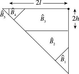
We define a two-parameter parametric dressed domain, the base triangle. For parameters l+𝑙subscriptl\in\mathbb{R}_{+} and h[0,αl]0𝛼𝑙h\in[0,\alpha l], we define a prototype ^(l,h)=(B^,𝐁^,ρ)^𝑙^B^𝐁𝜌\widehat{{\mathcal{B}}}(l,h)=(\widehat{\mathrm{B}},\widehat{\mathbf{B}},\rho) to represent its equivalence class with respect to 𝔊𝔊\mathfrak{G}. The dressed domain induced on the atom R1(s)subscript𝑅1𝑠R_{1}(s) of \mathcal{R} will be shown below to be congruent to ^(1,s)^1𝑠\widehat{{\mathcal{B}}}(1,s).

The tiling 𝐁^^𝐁\widehat{\mathbf{B}} is illustrated in figure 5. The defining data are presented in Table 1. For simplicity, we choose a frame of reference with the right-angle vertex of B^^B\widehat{\mathrm{B}} at the origin and the remaining vertices at points of the negative x𝑥x and y𝑦y axes.

Table 1: Tiling table of the prototype base triangle ^(l,h)^𝑙\widehat{{\mathcal{B}}}(l,h), for 0<h/l<α0𝑙𝛼0<h/l<\alpha.
Source PolygonInitial PlacementDestinationTileQ#Parameters𝚁#TranslationTile𝚁#B^1αl+βh7(0,0)B^11αβlβh2(αlh,αβl+βh)𝚄1B^12B^272lαh0(2l+αh,2h)𝚄1B^23B^36αlh,h0(h,h)𝚄1B^32B^47αh5(2l+αh,0)𝚄1B^41B^51βh7(2l,0)𝚄1B^50missing-subexpressionmissing-subexpressionmissing-subexpressionmissing-subexpressionmissing-subexpressionmissing-subexpressionmissing-subexpressionSource PolygonInitial PlacementDestinationmissing-subexpressionmissing-subexpressionmissing-subexpressionmissing-subexpressionmissing-subexpressionmissing-subexpressionmissing-subexpressionTilesubscript𝑄#Parameterssubscript𝚁#TranslationTilesubscript𝚁#missing-subexpressionmissing-subexpressionmissing-subexpressionmissing-subexpressionmissing-subexpressionmissing-subexpressionmissing-subexpressionmissing-subexpressionmissing-subexpressionmissing-subexpressionmissing-subexpressionmissing-subexpressionmissing-subexpressionmissing-subexpression^B1𝛼𝑙𝛽700missing-subexpressionmissing-subexpressionmissing-subexpressionmissing-subexpressionmissing-subexpressionmissing-subexpressionmissing-subexpressionmissing-subexpressionmissing-subexpressionmissing-subexpressionmissing-subexpressionmissing-subexpressionmissing-subexpressionmissing-subexpressionsubscript^𝐵11𝛼𝛽𝑙𝛽2𝛼𝑙𝛼𝛽𝑙𝛽subscript𝚄1subscript^𝐵12missing-subexpressionmissing-subexpressionmissing-subexpressionmissing-subexpressionmissing-subexpressionmissing-subexpressionmissing-subexpressionsubscript^𝐵272𝑙𝛼02𝑙𝛼2subscript𝚄1subscript^𝐵23missing-subexpressionmissing-subexpressionmissing-subexpressionmissing-subexpressionmissing-subexpressionmissing-subexpressionmissing-subexpressionsubscript^𝐵36𝛼𝑙0subscript𝚄1subscript^𝐵32missing-subexpressionmissing-subexpressionmissing-subexpressionmissing-subexpressionmissing-subexpressionmissing-subexpressionmissing-subexpressionsubscript^𝐵47𝛼52𝑙𝛼0subscript𝚄1subscript^𝐵41missing-subexpressionmissing-subexpressionmissing-subexpressionmissing-subexpressionmissing-subexpressionmissing-subexpressionmissing-subexpressionsubscript^𝐵51𝛽72𝑙0subscript𝚄1subscript^𝐵50\begin{array}[]{|c|c|c|c|c|c|c|}\hline\cr\vrule\lx@intercol\hfil\mbox{Source Polygon}\hfil\lx@intercol\vrule\lx@intercol&\vrule\lx@intercol\hfil\mbox{Initial Placement}\hfil\lx@intercol\vrule\lx@intercol&\vrule\lx@intercol\hfil\mbox{Destination}\hfil\lx@intercol\vrule\lx@intercol\\ \hline\cr\mbox{Tile}&Q_{\#}&\mbox{Parameters}&{\tt R}_{\#}&\mbox{Translation}&\mbox{Tile}&{\tt R}_{\#}\\ \hline\cr\hline\cr\widehat{\mathrm{B}}&1&\alpha l+\beta h&7&(0,0)&\mbox{---}&\mbox{---}\\ \hline\cr\hline\cr\widehat{B}_{1}&1&\alpha\beta l-\beta h&2&(-\alpha l-h,-\alpha\beta l+\beta h)&\mathtt{U}_{1}\widehat{B}_{1}&2\\ \hline\cr\widehat{B}_{2}&7&2l-\alpha h&0&(-2l+\alpha h,-2h)&\mathtt{U}_{1}\widehat{B}_{2}&3\\ \hline\cr\widehat{B}_{3}&6&\alpha l-h,h&0&(-h,-h)&\mathtt{U}_{1}\widehat{B}_{3}&2\\ \hline\cr\widehat{B}_{4}&7&\alpha h&5&(-2l+\alpha h,0)&\mathtt{U}_{1}\widehat{B}_{4}&1\\ \hline\cr\widehat{B}_{5}&1&\beta h&7&(-2l,0)&\mathtt{U}_{1}\widehat{B}_{5}&0\\ \hline\cr\end{array}

In the table, the atoms of 𝐁^^𝐁\widehat{\mathbf{B}} and their span are listed by giving their respective orientations and translation vectors relative to a representative tile in the catalogue of Appendix A. For example, we learn from table 1 that

B^1=𝚃𝐝𝚁2Q1(αβlβh),subscript^𝐵1subscript𝚃𝐝subscript𝚁2subscript𝑄1𝛼𝛽𝑙𝛽\widehat{B}_{1}=\mathtt{T}_{\mathbf{d}}\,\mathtt{R}_{2}\,Q_{1}(\alpha\beta l-\beta h),

where 𝐝=(αlh,αβl+βh)𝐝𝛼𝑙𝛼𝛽𝑙𝛽\mathbf{d}=(-\alpha l-h,-\alpha\beta l+\beta h) is the location of the offset tile’s anchor point (local origin; see Appendix A). The isometry ρ1subscript𝜌1\rho_{1} associated with atom B^1subscript^𝐵1\widehat{B}_{1} is uniquely specified by the information listed in the last two columns. Because 𝐝𝐝\mathbf{d} lies on the symmetry line of the tile, it is taken into 𝚄1(𝐝)subscript𝚄1𝐝\mathtt{U}_{1}(\mathbf{d}) by ρ1subscript𝜌1\rho_{1}. More generally, if n1subscript𝑛1n_{1} is the rotation index of the last column of the table, we calculate
ρ1=T𝚄1𝐝𝚁n1𝐝𝚁n1.subscript𝜌1subscript𝑇subscript𝚄1𝐝subscript𝚁subscript𝑛1𝐝subscript𝚁subscript𝑛1\rho_{1}=T_{\mathtt{U}_{1}\mathbf{d}-\mathtt{R}_{n_{1}}\mathbf{d}}\,\mathtt{R}_{n_{1}}.
Refer to caption
Figure 5: The prototype base triangle ^(l,h)^𝑙\widehat{{\mathcal{B}}}(l,h) for 0<h/l<α0𝑙𝛼0<h/l<\alpha.

The definition of the base triangle can be extended to the boundary of the parametric domain. This domain has two atoms for h=00h=0 (and any l𝑙l) and three for h=αl𝛼𝑙h=\alpha l; the atoms are still described by table 1 with the stipulation that all zero-parameter entries are to be deleted.

The following result establishes the dynamics of the base triangle, which is the basis of the renormalization process.

Proposition 1

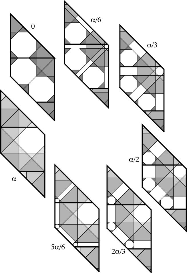
For all sI𝑠𝐼s\in I, let (s)=(R(s),(Ri(s)),(ρi(s)))𝑠R𝑠subscript𝑅𝑖𝑠subscript𝜌𝑖𝑠\mathcal{R}(s)=(\mathrm{R}(s),(R_{i}(s)),(\rho_{i}(s))) be the parametric dressed rhombus defined in equations (7)–(9). Then the atom R1(s)subscript𝑅1𝑠R_{1}(s), equipped with the return map induced by ρ(s)𝜌𝑠\rho(s), is a dressed subdomain \mathcal{B} congruent to the prototype base triangle ^(1,s)^1𝑠\widehat{\mathcal{B}}(1,s). The rhombus R(s)R𝑠\mathrm{R}(s) is tiled by the return orbits of the atoms of \mathcal{B} and also of the periodic tiles

Π1=𝚃(1s,1βs)Q10(s,αs),Π2=𝚃(1s,ββs)Q5(αs),Π3=𝚃(ωs,1βs)Q5(s),subscriptΠ1subscript𝚃1𝑠1𝛽𝑠subscript𝑄10𝑠𝛼𝑠subscriptΠ2subscript𝚃1𝑠𝛽𝛽𝑠subscript𝑄5𝛼𝑠subscriptΠ3subscript𝚃𝜔𝑠1𝛽𝑠subscript𝑄5𝑠\begin{array}[]{l}\Pi_{1}=\mathtt{T}_{(-1-s,1-\beta s)}\,Q_{10}(s,\alpha-s),\\ \Pi_{2}=\mathtt{T}_{(-1-s,-\beta-\beta s)}\,Q_{5}(\alpha-s),\\ \Pi_{3}=\mathtt{T}_{(\omega-s,1-\beta s)}\,Q_{5}(s),\end{array}

apart from a set of zero measure. The incidence matrix for the return orbits of the atoms is:

(111118524652222).111118524652222\left(\begin{array}[]{ccccc}1&1&1&1&1\\ 8&5&2&4&6\\ 5&2&2&2&2\end{array}\right).

Proof. The proof is a straightforward application of the direct iteration method described in section 2.5. The initial and final tiles of the return orbits can be gleaned from table 1, and we know that the periodic orbits should begin and end on Πk,k=1,2,3formulae-sequencesubscriptΠ𝑘𝑘123\Pi_{k},\,k=1,2,3. In the course of constructing the return orbits, we keep track of the atoms visited, obtaining at the end the symbolic paths and incidence matrices of the orbits. By adding up the areas of the tiles of all the orbits, and comparing with the total area of the parent domain, we prove the completeness of the tiling.

The details of the computer-assisted calculation may be found in the Electronic Supplement[6]. \Box

The tiling is illustrated for several values of s𝑠s in figure 6. The reader may find it instructive to follow each of the orbits around the rhombus, applying ‘by eye’ the product of local and global involutions at each step.
Refer to caption
Figure 6: Tiling of the rhombus RR\mathrm{R} by return orbits of the atoms of R1subscript𝑅1R_{1} (shades of gray) and the periodic tiles Π1,Π2,Π3subscriptΠ1subscriptΠ2subscriptΠ3\Pi_{1},\Pi_{2},\Pi_{3} (white), for equally spaced values of s=h/l𝑠𝑙s=h/l in I=[0,α]𝐼0𝛼I=[0,\alpha]. The three atoms of \mathcal{R} have been drawn with thicker boundaries.

4 Main results

We now state the main results of our investigation. We begin by defining the renormalization functions f𝑓f and r=f2𝑟superscript𝑓2r=f^{2} (see figures 2 and 7), for all sI=[0,α]𝑠𝐼0𝛼s\in I=[0,\alpha]:

f(0)=f(α)=0,𝑓0𝑓𝛼0f(0)=f(\alpha)=0,
f(s)=ω|i|+1{(Δis)sIi,i<0(sβ)sI0(sΔi)sIi,i>0,𝑓𝑠superscript𝜔𝑖1casessubscriptΔ𝑖𝑠formulae-sequence𝑠subscript𝐼𝑖𝑖0𝑠𝛽𝑠subscript𝐼0𝑠subscriptΔ𝑖formulae-sequence𝑠subscript𝐼𝑖𝑖0f(s)=\omega^{|i|+1}\left\{\begin{array}[]{ll}(\Delta_{i}-s)&s\in I_{i},\;i<0\\ (s-\beta)&s\in I_{0}\\ (s-\Delta_{i})&s\in I_{i},\;i>0,\end{array}\right. (11)

where

Ii={(Δi1,Δi]i<0(β,1)i=0[Δi,Δi+1)i>0Δi={β|i|i<0β,i=0αβ|i|i>0formulae-sequencesubscript𝐼𝑖casessubscriptΔ𝑖1subscriptΔ𝑖𝑖0𝛽1𝑖0subscriptΔ𝑖subscriptΔ𝑖1𝑖0subscriptΔ𝑖casessuperscript𝛽𝑖𝑖0𝛽𝑖0𝛼superscript𝛽𝑖𝑖0I_{i}=\left\{\begin{array}[]{ll}(\Delta_{i-1},\Delta_{i}]&i<0\\ (\beta,1)&i=0\\ \left[\Delta_{i},\Delta_{i+1})\right.&i>0\end{array}\right.\qquad\Delta_{i}=\left\{\begin{array}[]{ll}\beta^{|i|}&i<0\\ \beta,&i=0\\ \alpha-\beta^{|i|}&i>0\end{array}\right. (12)

and

r(0)=r(α)=0,𝑟0𝑟𝛼0r(0)=r(\alpha)=0,
r(s)=ω|i|+|j|+2{(Δi,js)sIi,j,j<0 or (j=0 and i<0),(sΔi,j)sIi,j,j>0 or (j=0 and i0),𝑟𝑠superscript𝜔𝑖𝑗2casessubscriptΔ𝑖𝑗𝑠formulae-sequence𝑠subscript𝐼𝑖𝑗𝑗0 or 𝑗0 and 𝑖0𝑠subscriptΔ𝑖𝑗formulae-sequence𝑠subscript𝐼𝑖𝑗𝑗0 or 𝑗0 and 𝑖0r(s)=\omega^{|i|+|j|+2}\left\{\begin{array}[]{ll}(\Delta_{i,j}-s)&s\in I_{i,j},\quad j<0\mbox{ or }(j=0\mbox{ and }i<0),\\ (s-\Delta_{i,j})&s\in I_{i,j},\quad j>0\mbox{ or }(j=0\mbox{ and }i\geq 0),\end{array}\right. (13)

where

Ii,j={(Δi,j1,Δi,j]j<0(Δi,1,Δi,0)j=0,i<0(Δi,0,Δi,1)j=0,i0[Δi,j,Δi,j+1)j>0,subscript𝐼𝑖𝑗casessubscriptΔ𝑖𝑗1subscriptΔ𝑖𝑗𝑗0subscriptΔ𝑖1subscriptΔ𝑖0formulae-sequence𝑗0𝑖0subscriptΔ𝑖0subscriptΔ𝑖1formulae-sequence𝑗0𝑖0subscriptΔ𝑖𝑗subscriptΔ𝑖𝑗1𝑗0I_{i,j}=\left\{\begin{array}[]{ll}(\Delta_{i,j-1},\Delta_{i,j}]&j<0\\ (\Delta_{i,-1},\Delta_{i,0})&j=0,\,i<0\\ (\Delta_{i,0},\Delta_{i,1})&j=0,\,i\geqslant 0\\ \left[\Delta_{i,j},\Delta_{i,j+1})\right.&j>0,\end{array}\right.
Δi,j={β|i|+1+β|i|+|j|+1i0,j0β|i|β|i|+|j|+1i<0,j>0αΔi,ji>0 or (i=0 and j>0).subscriptΔ𝑖𝑗casessuperscript𝛽𝑖1superscript𝛽𝑖𝑗1formulae-sequence𝑖0𝑗0superscript𝛽𝑖superscript𝛽𝑖𝑗1formulae-sequence𝑖0𝑗0𝛼subscriptΔ𝑖𝑗𝑖0 or 𝑖0 and 𝑗0\Delta_{i,j}=\left\{\begin{array}[]{ll}\beta^{|i|+1}+\beta^{|i|+|j|+1}&i\leqslant 0,\,j\leqslant 0\\ \beta^{|i|}-\beta^{|i|+|j|+1}&i<0,\,j>0\\ \alpha-\Delta_{-i,-j}&i>0\mbox{ or }(i=0\mbox{ and }j>0).\end{array}\right.
Refer to caption
Figure 7: The piecewise-affine renormalization function r=f2𝑟superscript𝑓2r=f^{2}

.

The following two theorems constitute our main results.

Theorem 1

Let {\mathcal{B}} be a parametric base triangle congruent to the prototype ^(l,sl)^𝑙𝑠𝑙\widehat{{\mathcal{B}}}(l,sl). Then {\mathcal{B}} is renormalizable for all positive real l𝑙l and sI𝑠𝐼s\in I. Specifically:

i)i) For s{0,α}𝑠0𝛼s\in\{0,\alpha\}, {\mathcal{B}} has a dressed subdomain superscript{\mathcal{B}}^{*} congruent to ^(κ(s)l,0)^𝜅𝑠𝑙0\widehat{{\mathcal{B}}}(\kappa(s)l,0), with

κ(0)=β,κ(α)=1.formulae-sequence𝜅0𝛽𝜅𝛼1\kappa(0)=\beta,\qquad\kappa(\alpha)=1.

The parity π()𝜋superscript\pi({\mathcal{B}}^{*}) is π()𝜋-\pi({\mathcal{B}}) for s=0𝑠0s=0 and π()𝜋\pi({\mathcal{B}}) for s=α𝑠𝛼s=\alpha. The return-map orbits of the atoms of superscript{\mathcal{B}}^{*}, together with those of a finite number of periodic tiles, tile the spanning triangle of {\mathcal{B}}, up to a set of measure zero.

ii)ii) For all i{0}𝑖0i\in\mathbb{Z}\setminus\{0\} and s=Δi𝑠subscriptΔ𝑖s=\Delta_{i}, as defined in (12), the domain {\mathcal{B}} has two dressed subdomains, superscript{\mathcal{B}}^{*} and superscript{\mathcal{B}}^{\dagger} congruent, respectively, to ^(κ(Δi)l,0)^superscript𝜅subscriptΔ𝑖𝑙0\widehat{{\mathcal{B}}}(\kappa^{*}(\Delta_{i})l,0) and ^(κ(Δi)l,0)^superscript𝜅subscriptΔ𝑖𝑙0\widehat{{\mathcal{B}}}(\kappa^{\dagger}(\Delta_{i})l,0), with

κ(Δi)=β|i|/α,κ(Δi)=β|i|+2/α.formulae-sequencesuperscript𝜅subscriptΔ𝑖superscript𝛽𝑖𝛼superscript𝜅subscriptΔ𝑖superscript𝛽𝑖2𝛼\kappa^{*}(\Delta_{i})=\beta^{|i|}/\alpha,\qquad\kappa^{\dagger}(\Delta_{i})=\beta^{|i|+2}/\alpha.

The parities π()𝜋superscript\pi({\mathcal{B}}^{*}) and π()𝜋superscript\pi({\mathcal{B}}^{\dagger}) are both (1)|i|+1π()superscript1𝑖1𝜋(-1)^{|i|+1}\pi({\mathcal{B}}). The return-map orbits of the atoms of superscript{\mathcal{B}}^{*} and superscript{\mathcal{B}}^{\dagger}, together with those of a finite number of periodic tiles, tile the spanning triangle of {\mathcal{B}}, up to a set of measure zero.

iii)iii) For all i,j𝑖𝑗i,j\in\mathbb{Z} and sIi,j𝑠subscript𝐼𝑖𝑗s\in I_{i,j}, the dressed domain {\mathcal{B}} has a dressed subdomain superscript{\mathcal{B}}^{*} congruent to ^(l,sl),l=κ(s)l,s=r(s)formulae-sequence^superscript𝑙superscript𝑠superscript𝑙superscript𝑙𝜅𝑠𝑙superscript𝑠𝑟𝑠\widehat{{\mathcal{B}}}(l^{*},s^{*}l^{*}),\;l^{*}=\kappa(s)l,\;s^{*}=r(s), with r(s)𝑟𝑠r(s) given by (13) and

κ(s)=β|i|+|j|+2,π()=(1)|i|+|j|π().formulae-sequence𝜅𝑠superscript𝛽𝑖𝑗2𝜋superscriptsuperscript1𝑖𝑗𝜋\kappa(s)=\beta^{|i|+|j|+2},\qquad\pi({\mathcal{B}}^{*})=(-1)^{|i|+|j|}\pi({\mathcal{B}}).

The return-map orbits of the atoms of superscript{\mathcal{B}}^{*}, together with those of a finite number of periodic tiles, tile the spanning triangle of {\mathcal{B}}, up to a set of measure zero. The tilings vary continuously with respect to sIi,j𝑠subscript𝐼𝑖𝑗s\in I_{i,j}, with the return paths (hence the incidence matrix) constant over the interior of the interval.

There is a tight connection between strict renormalizability and the field (2)2\mathbb{Q}(\sqrt{2}), due to the following result.

Theorem 2

The renormalization function f𝑓f is conjugate to a left shift acting in a space of one-sided symbol sequences with alphabet {,+}\mathbb{Z}\cup\{-\infty,+\infty\}. A point sI𝑠𝐼s\in I is eventually periodic under f𝑓f if and only if s(2)𝑠2s\in\mathbb{Q}(\sqrt{2}). Hence the set of values of s𝑠s for which a base triangle congruent to ^(l,sl)^𝑙𝑠𝑙\widehat{{\mathcal{B}}}(l,sl) is strictly renormalizable is (2)I2𝐼\mathbb{Q}(\sqrt{2})\cap I.

Theorem 1 will be proved from the analysis of the return-map dynamics. Before that rather lengthy analysis, we will prove theorem 2 and study some interesting properties of the function f𝑓f and its symbolic dynamics.

5 Symbolic dynamics

In this section we introduce a symbolic dynamics for f𝑓f which will give us a useful expansion for sI𝑠𝐼s\in I —equation (21). This is a variant of the so-called Lüroth expansions [15, 8, 3].

The renormalization map f𝑓f, see (11) and figure 2, is piecewise-affine, and its restriction to the interval Iisubscript𝐼𝑖I_{i} has slope ±ω|i|+1plus-or-minussuperscript𝜔𝑖1\pm\omega^{|i|+1}. Since ω>1𝜔1\omega>1, this map is expanding, and since the length of Ii±superscriptsubscript𝐼𝑖plus-or-minusI_{i}^{\pm} is equal to αβ|i|+1=α/ω|i|+1𝛼superscript𝛽𝑖1𝛼superscript𝜔𝑖1\alpha\beta^{|i|+1}=\alpha/\omega^{|i|+1}, we see that f(Ii)=I𝑓subscript𝐼𝑖𝐼f(I_{i})=I (with the origin missing if i=0𝑖0i=0). It follows that f𝑓f preserves the Lebesgue measure.

Next we define the function i:I{,+}:𝑖𝐼i:I\to\mathbb{Z}\cup\{-\infty,+\infty\} which assigns to each s𝑠s the interval Iisubscript𝐼𝑖I_{i} to which it belongs. Explicitly,

i(s)={logβ(s)0<sβlogβ(αs)β<s<αs=0+s=α.𝑖𝑠casessubscript𝛽𝑠0𝑠𝛽subscript𝛽𝛼𝑠𝛽𝑠𝛼𝑠0𝑠𝛼i(s)=\left\{\begin{array}[]{ll}\lfloor\log_{\beta}(s)\rfloor&\qquad 0<s\leqslant\beta\\ \lfloor\log_{\beta}(\alpha-s)\rfloor&\qquad\beta<s<\alpha\\ -\infty&\qquad s=0\\ +\infty&\qquad s=\alpha.\end{array}\right.\\ (14)

In terms of this function, f𝑓f can be rewritten as

f(s)={σ(i(s))ω|i(s)|+1(sΔi(s))s0,α0s=0,α,𝑓𝑠cases𝜎𝑖𝑠superscript𝜔𝑖𝑠1𝑠subscriptΔ𝑖𝑠𝑠0𝛼0𝑠0𝛼f(s)=\left\{\begin{array}[]{ll}\sigma(i(s))\,\omega^{|i(s)|+1}\,\bigl{(}s-\Delta_{i(s)})&\quad s\not=0,\alpha\\ 0&\quad s=0,\alpha,\end{array}\right. (15)

where

σ(i)={1i<01i0.𝜎𝑖cases1𝑖01𝑖0\sigma(i)=\left\{\begin{array}[]{ll}-1&i<0\\ 1&i\geqslant 0.\end{array}\right. (16)

Let us now consider the orbit of f𝑓f with initial condition s0=sIsubscript𝑠0𝑠𝐼s_{0}=s\in I. For all k0𝑘0k\geqslant 0 we let sk+1=f(sk)subscript𝑠𝑘1𝑓subscript𝑠𝑘s_{k+1}=f(s_{k}). With the notation

ik=i(sk),σk=σ(ik),πk=α(1+σk)/2,formulae-sequencesubscript𝑖𝑘𝑖subscript𝑠𝑘formulae-sequencesubscript𝜎𝑘𝜎subscript𝑖𝑘subscript𝜋𝑘𝛼1subscript𝜎𝑘2i_{k}=i(s_{k}),\qquad\sigma_{k}=\sigma(i_{k}),\qquad\pi_{k}=\alpha(1+\sigma_{k})/2, (17)

equation (15) becomes

sk+1={σkω|ik|+1(skπk+σkβ|ik|)sk0,α0sk=0,α.subscript𝑠𝑘1casessubscript𝜎𝑘superscript𝜔subscript𝑖𝑘1subscript𝑠𝑘subscript𝜋𝑘subscript𝜎𝑘superscript𝛽subscript𝑖𝑘subscript𝑠𝑘0𝛼0subscript𝑠𝑘0𝛼s_{k+1}=\left\{\begin{array}[]{ll}\sigma_{k}\omega^{|i_{k}|+1}\,(s_{k}-\pi_{k}+\sigma_{k}\beta^{|i_{k}|})&\quad s_{k}\not=0,\alpha\\ 0&\quad s_{k}=0,\alpha.\end{array}\right. (18)

In this way, every sI𝑠𝐼s\in I is associated with a unique sequence

(i0,i1,i2,)subscript𝑖0subscript𝑖1subscript𝑖2(i_{0},i_{1},i_{2},\ldots\,) (19)

with ik{,+}subscript𝑖𝑘i_{k}\in\mathbb{Z}\cup\{-\infty,+\infty\}. The only constraints which we impose on these sequences is that the sub-strings (,r),rminus-or-plus𝑟𝑟(\mp\infty,r),\;r\neq-\infty are forbidden, and that the symbol ++\infty can only appear as the leading symbol: (+,,)(+\infty,-\infty,\ldots). In the space of such sequences, a left shift is conjugate to the map f𝑓f on I𝐼I.

To establish that each allowed sequence (19) corresponds to a unique s𝑠s, we begin with the sequences (,,,)minus-or-plus(\mp\infty,-\infty,-\infty,\ldots), which represents exclusively the value 00 (negative sign) and α𝛼\alpha (positive sign). All other sequences either have no symbols -\infty, or else have an infinite tail of -\infty symbols preceded by a finite sequence in which minus-or-plus\mp\infty does not appear. In either case, we can assume sk0,αsubscript𝑠𝑘0𝛼s_{k}\neq 0,\alpha and invert (18) to obtain

sk=πkσkβ|ik|+σkβ|ik|+1sk+1.subscript𝑠𝑘subscript𝜋𝑘subscript𝜎𝑘superscript𝛽subscript𝑖𝑘subscript𝜎𝑘superscript𝛽subscript𝑖𝑘1subscript𝑠𝑘1s_{k}=\pi_{k}-\sigma_{k}\beta^{|i_{k}|}+\sigma_{k}\beta^{|i_{k}|+1}s_{k+1}. (20)

Iterating, we find:

s0subscript𝑠0\displaystyle s_{0} =\displaystyle= π0σ0β|i0|+σ0β|i0|+1s1subscript𝜋0subscript𝜎0superscript𝛽subscript𝑖0subscript𝜎0superscript𝛽subscript𝑖01subscript𝑠1\displaystyle\pi_{0}-\sigma_{0}\beta^{|i_{0}|}+\sigma_{0}\beta^{|i_{0}|+1}s_{1}
=\displaystyle= π0σ0(ωπ1)β|i0|+1σ0σ1β|i0|+|i1|+1+σ0σ1β|i0|+|i1|+2s2.subscript𝜋0subscript𝜎0𝜔subscript𝜋1superscript𝛽subscript𝑖01subscript𝜎0subscript𝜎1superscript𝛽subscript𝑖0subscript𝑖11subscript𝜎0subscript𝜎1superscript𝛽subscript𝑖0subscript𝑖12subscript𝑠2\displaystyle\pi_{0}-\sigma_{0}(\omega-\pi_{1})\beta^{|i_{0}|+1}-\sigma_{0}\sigma_{1}\beta^{|i_{0}|+|i_{1}|+1}+\sigma_{0}\sigma_{1}\beta^{|i_{0}|+|i_{1}|+2}s_{2}.

An easy induction gives

s=s0=π0ΛΛ=n1anβn+bn,𝑠subscript𝑠0subscript𝜋0ΛΛsubscript𝑛1subscript𝑎𝑛superscript𝛽𝑛subscript𝑏𝑛s=s_{0}=\pi_{0}-\Lambda\hskip 40.0pt\Lambda=\sum_{n\geqslant 1}a_{n}\beta^{n+b_{n}}, (21)

where

an=(ωπn)k<nσkbn=k<n|ik|.subscript𝑎𝑛𝜔subscript𝜋𝑛subscriptproduct𝑘𝑛subscript𝜎𝑘subscript𝑏𝑛subscript𝑘𝑛subscript𝑖𝑘a_{n}=(\omega-\pi_{n})\prod_{k<n}\sigma_{k}\hskip 40.0ptb_{n}=\sum_{k<n}|i_{k}|. (22)

The sequence (bn)subscript𝑏𝑛(b_{n}) is non-negative and non-decreasing, and we have bn0subscript𝑏𝑛0b_{n}\equiv 0 only for the fixed point s=2/2𝑠22s=\sqrt{2}/2. The sequence (an)subscript𝑎𝑛(a_{n}) depends only on the σksubscript𝜎𝑘\sigma_{k}s; indeed,

ωπn={ωσn=11σn=+1.𝜔subscript𝜋𝑛cases𝜔subscript𝜎𝑛11subscript𝜎𝑛1\omega-\pi_{n}=\left\{\begin{array}[]{ll}\omega&\quad\sigma_{n}=-1\\ 1&\quad\sigma_{n}=+1.\end{array}\right. (23)

Thus an{±1,±ω}subscript𝑎𝑛plus-or-minus1plus-or-minus𝜔a_{n}\in\{\pm 1,\pm\omega\}.

The sum in (21) is absolutely convergent, and it provides an expansion for any s[0,α)𝑠0𝛼s\in[0,\alpha). On the other hand, having excluded ++\infty from all but one sequence, distinct sequences correspond to distinct values of s[0,α]𝑠0𝛼s\in[0,\alpha]. This completes the proof of the claimed bi-unique correspondence.

The expansion (21) is finite if the orbit of s0subscript𝑠0s_{0} reaches the origin, and infinite otherwise. In the former case ΛΛ\Lambda is a finite sum of elements of [α]delimited-[]𝛼\mathbb{Z}[\alpha], and hence s[α]𝑠delimited-[]𝛼s\in\mathbb{Z}[\alpha]. If the sequence (19) is eventually periodic with limiting period N𝑁N, then the sequence ansubscript𝑎𝑛a_{n} is eventually periodic with the same transient and period N𝑁N or 2N2𝑁2N, while the sequence bnsubscript𝑏𝑛b_{n} eventually becomes the sum of an affine function plus a periodic function with period dividing N𝑁N. Then the sum ΛΛ\Lambda decomposes into the sum of finitely many geometric progressions, and so ΛΛ\Lambda, and hence s𝑠s, belong to (α)𝛼\mathbb{Q}(\alpha).

In the next section we shall demonstrate that the converse is also true, namely that any s(α)[0,α]𝑠𝛼0𝛼s\in\mathbb{Q}(\alpha)\cap[0,\alpha] has an eventually periodic symbol sequence of the type (19).

6 Lattice dynamics

Let the ring [α]delimited-[]𝛼\mathbb{Z}[\alpha] and the interval I𝐼I be given by (1) and (10), respectively. For d1𝑑1d\geqslant 1, we define

d=1d[α]Isubscript𝑑1𝑑delimited-[]𝛼𝐼\mathcal{M}_{d}=\frac{1}{d}\mathbb{Z}[\alpha]\cap I (24)

which is the restriction to I𝐼I of the module d1[α]superscript𝑑1delimited-[]𝛼d^{-1}\mathbb{Z}[\alpha]. Because f(s)𝑓𝑠f(s) is obtained from s𝑠s by ring operations in [α]delimited-[]𝛼\mathbb{Z}[\alpha], and f(I)=I𝑓𝐼𝐼f(I)=I, we have that f(d)d𝑓subscript𝑑subscript𝑑f(\mathcal{M}_{d})\subset\mathcal{M}_{d}. We have established the first part of the following lemma:

Lemma 1

For each d𝑑d, we have

f(d)d,f1(d{α})d.formulae-sequence𝑓subscript𝑑subscript𝑑superscript𝑓1subscript𝑑𝛼subscript𝑑f(\mathcal{M}_{d})\subset\mathcal{M}_{d},\qquad f^{-1}(\mathcal{M}_{d}\setminus\{\alpha\})\subset\mathcal{M}_{d}.

Proof. It remains to show the invariance with respect to f1superscript𝑓1f^{-1}. In the statement of the lemma, the element α1𝛼subscript1\alpha\in\mathcal{M}_{1} had to be removed since it is not in the domain of the function f1superscript𝑓1f^{-1}.

We have 010subscript10\in\mathcal{M}_{1}, and, by construction we have

f1({0})={,Δ2,Δ1,Δ0,Δ1,Δ2,}{0,α}1.superscript𝑓10subscriptΔ2subscriptΔ1subscriptΔ0subscriptΔ1subscriptΔ20𝛼subscript1f^{-1}(\{0\})=\{\ldots,\Delta_{-2},\Delta_{1},\Delta_{0},\Delta_{1},\Delta_{2},\ldots\}\cup\{0,\alpha\}\subset\mathcal{M}_{1}.

Let now s0,α𝑠0𝛼s\not=0,\alpha and let s=f(s)dsuperscript𝑠𝑓𝑠subscript𝑑s^{\prime}=f(s)\in\mathcal{M}_{d}. Using (11) we find

s=sσ(i(s))β|i(s)|+1+Δi(s).𝑠superscript𝑠𝜎𝑖𝑠superscript𝛽𝑖𝑠1subscriptΔ𝑖𝑠s=s^{\prime}\sigma(i(s))\beta^{|i(s)|+1}+\Delta_{i(s)}.

For any choice of the values of i𝑖i, we see that s𝑠s is an affine function of ssuperscript𝑠s^{\prime} with coefficients in [α]delimited-[]𝛼\mathbb{Z}[\alpha]. Since [α]/ddelimited-[]𝛼𝑑\mathbb{Z}[\alpha]/d is a module over [α]delimited-[]𝛼\mathbb{Z}[\alpha], it follows that sd𝑠subscript𝑑s\in\mathcal{M}_{d} (see (24)). \Box


Since, by the lemma, the inverse function cannot increase the denominator, then the forward function cannot decrease it. This can be rephrased as follows. For any ξ(α)𝜉𝛼\xi\in\mathbb{Q}(\alpha), let d=d(ξ)superscript𝑑superscript𝑑𝜉d^{*}=d^{*}(\xi) be the smallest natural number d𝑑d such that ξd𝜉subscript𝑑\xi\in\mathcal{M}_{d}. Then dsuperscript𝑑d^{*} is a constant of the motion for the map f𝑓f.

For sd𝑠subscript𝑑s\in\mathcal{M}_{d} we let ζ=sd𝜁𝑠𝑑\zeta=sd. Then ζ[α]dI𝜁delimited-[]𝛼𝑑𝐼\zeta\in\mathbb{Z}[\alpha]\cap dI, and alongside the interval map sf(s)maps-to𝑠𝑓𝑠s\mapsto f(s), we have the ring map

fd:[α][α]ζσ(i(s))ω|i(s)|+1(ζdΔi(s))s=1dζ:subscript𝑓𝑑formulae-sequencedelimited-[]𝛼delimited-[]𝛼formulae-sequencemaps-to𝜁𝜎𝑖𝑠superscript𝜔𝑖𝑠1𝜁𝑑subscriptΔ𝑖𝑠𝑠1𝑑𝜁f_{d}:\mathbb{Z}[\alpha]\to\mathbb{Z}[\alpha]\qquad\zeta\mapsto\sigma(i(s))\omega^{|i(s)|+1}\left(\zeta-d\Delta_{i(s)}\right)\quad s=\frac{1}{d}\,\zeta (25)

(with fd(0)=fd(dα)=0subscript𝑓𝑑0subscript𝑓𝑑𝑑𝛼0f_{d}(0)=f_{d}(d\alpha)=0) which represents the restriction of f𝑓f to dsubscript𝑑\mathcal{M}_{d} after clearing denominators.

Conclusion of the proof of theorem 2. We introduce the natural bijection

ϕ:[α]2m+nα(m,n):italic-ϕformulae-sequencedelimited-[]𝛼superscript2maps-to𝑚𝑛𝛼𝑚𝑛\phi:\mathbb{Z}[\alpha]\to\mathbb{Z}^{2}\qquad m+n\alpha\mapsto(m,n)

which conjugates fdsubscript𝑓𝑑f_{d} to a lattice map on 2superscript2\mathbb{Z}^{2}, for which still use the same symbol.

For any d>0𝑑0d>0, we define the infinite strip

Σd={(m,n)2:mnαm+dα},subscriptΣ𝑑conditional-set𝑚𝑛superscript2𝑚𝑛𝛼𝑚𝑑𝛼\Sigma_{d}=\left\{(m,n)\in\mathbb{Z}^{2}\,:\,-m\leqslant n\alpha\leqslant-m+d\alpha\right\},

which is invariant under fdsubscript𝑓𝑑f_{d} (because I𝐼I is invariant under f𝑓f).

We claim that all orbits of the map fdsubscript𝑓𝑑f_{d} are eventually periodic. Since Σd2subscriptΣ𝑑superscript2\Sigma_{d}\subset\mathbb{Z}^{2} this means that all orbits of fdsubscript𝑓𝑑f_{d} are bounded. Multiplication by ω𝜔\omega in [α]delimited-[]𝛼\mathbb{Z}[\alpha] induces a linear map M𝑀M on 2superscript2\mathbb{Z}^{2}, with eigenvalues ω,β𝜔𝛽-\omega,\beta. The lines αy=±x𝛼𝑦plus-or-minus𝑥\alpha y=\pm x are the corresponding eigendirections. Let zΣd𝑧subscriptΣ𝑑z\in\Sigma_{d}, and let (z,z+)subscript𝑧subscript𝑧(z_{-},z_{+}) be the components of z𝑧z with respect to a basis of eigenvectors.

Since the expanding eigendirection is transversal to ΣdsubscriptΣ𝑑\Sigma_{d}, there is a constant cdsubscript𝑐𝑑c_{d} such that |z+|<cdsubscript𝑧subscript𝑐𝑑|z_{+}|<c_{d}. So it suffices to show that the component zsubscript𝑧z_{-} remains bounded. For all z2𝑧superscript2z\in\mathbb{Z}^{2} and i0𝑖0i\geqslant 0 we have

|Mj+1(z)|β|z|<|z|.superscript𝑀𝑗1subscript𝑧𝛽subscript𝑧subscript𝑧|M^{j+1}(z)_{-}|\leqslant\beta|z_{-}|<|z_{-}|. (26)

Furthermore, from (12) we have that ω|i|+1Δisuperscript𝜔𝑖1subscriptΔ𝑖\omega^{|i|+1}\Delta_{i} is a monomial or binomial in ω𝜔\omega of degree at most |i|+1𝑖1{|i|+1} with coefficients 1,1,α11𝛼1,-1,\alpha. Defining

C=d(|ϕ(1)|+|ϕ(1)|+|ϕ(α)|)𝐶𝑑italic-ϕsubscript1italic-ϕsubscript1italic-ϕsubscript𝛼C=d\,(|\phi(1)_{-}|+|\phi(-1)_{-}|+|\phi(\alpha)_{-}|)

from (26) we have

|M|i|+1(ϕ(dΔi))||ϕ(dΔi)|C.superscript𝑀𝑖1subscriptitalic-ϕ𝑑subscriptΔ𝑖italic-ϕsubscript𝑑subscriptΔ𝑖𝐶|M^{|i|+1}(\phi(d\Delta_{i}))_{-}|\leqslant|\phi(d\Delta_{i})_{-}|\leqslant C. (27)

Finally, from (25), (26), and (27), we obtain

|fd(z)|β|z|+Csubscript𝑓𝑑subscript𝑧𝛽subscript𝑧𝐶|f_{d}(z)_{-}|\leqslant\beta|z_{-}|+C

and since β<1𝛽1\beta<1, for all sufficiently large |z|subscript𝑧|z_{-}| the map fdsubscript𝑓𝑑f_{d} is a contraction mapping. Thus its orbits are bounded hence eventually periodic.

This completes the proof of theorem 2. \Box

7 Overview of the renormalization dynamics

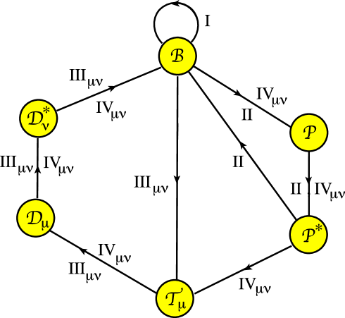
As a prelude to the proof of theorem 1, we now turn our attention to the dynamical underpinnings of the renormalizability of the parametric base triangle (l,s)𝑙𝑠{\mathcal{B}}(l,s). This analysis is based on the construction of the return-map tree through successive inductions on sub-domains, a process which is far more complex than one might guess from the simple functional form of the function r𝑟r. To account for the renormalizability of the entire parameter interval, ten distinct renormalization scenarios need to be considered, each characterized by the participation of distinctive parametric dressed domains. We have given such special domains names suggestive of their geometric structure: the pencil 𝒫𝒫{\mathcal{P}}, the fringed triangle 𝒯𝒯{\mathcal{T}}, and the double strip 𝒟𝒟{\mathcal{D}}. The induction sequence for each of the ten scenarios and the corresponding parameter intervals are specified in Table 2. In the labelling of the scenarios, Roman numerals I through IV are used to indicate the major classifications, with asterisks and binary subscripts μ,ν=±1𝜇𝜈plus-or-minus1\mu,\nu=\pm 1 indicating finer distinctions (to be clarified in the next section).

Table 2: Renormalization scenarios, each one corresponding to a simple closed loop on the renormalization graph of figure 8. (See also figures 9 and 10.)
Renormalization scenarioRanges of indicesI(±,0),(0,±)(1,j),(1,j),j=0,1,2,3(0,j),|j|2.II𝒫𝒫(i,j),(i,j),i2,3j2,(1,j),(1,j),j=1,2,(i,),(i,+),i1.IIIμν𝒯μ𝒟μ𝒟νμ=1:(0,±j),j3,μ=+1:(1,j),(1,j),j4,ν=(1)j.IVμν𝒫𝒯μ𝒟μ𝒟νμ=1:(i,j),(i,j),i1,j3,μ=+1:(i,j),(i,j),i2,j4,ν=(1)j.\begin{array}[]{|c|c|c|}\hline\cr\vrule\lx@intercol\hfil\mbox{Renormalization scenario}\hfil\lx@intercol\vrule\lx@intercol&\mbox{Ranges of indices}\\ \hline\cr\mbox{I}&{{\mathcal{B}}}\rightarrow{{\mathcal{B}}}&\begin{array}[]{c}(\pm\infty,0),\,(0,\pm\infty)\\ (-1,j),\;(1,-j),\quad j=0,1,2,3\\ (0,j),\quad|j|\leqslant 2.\end{array}\\ \hline\cr\mbox{II}&{{\mathcal{B}}}\rightarrow{\mathcal{P}}\rightarrow{\mathcal{P}}^{*}\rightarrow{{\mathcal{B}}}&\begin{array}[]{c}(i,j),(-i,-j),\;\;i\geqslant 2,\;\;-3\leqslant j\leqslant 2,\\ (1,j),\;(-1,-j),\quad j=1,2,\\ (-i,-\infty),\,(i,+\infty),\quad i\geqslant 1.\end{array}\\ \hline\cr\mbox{III}_{\mu\nu}&{{\mathcal{B}}}\rightarrow{\mathcal{T}}_{\mu}\rightarrow{\mathcal{D}}_{\mu}\rightarrow{\mathcal{D}}^{*}_{\nu}\rightarrow{{\mathcal{B}}}&\begin{array}[]{l}\mu=-1:\quad(0,\pm j),\quad j\geqslant 3,\\ \mu=+1:\quad(1,-j),\;(-1,j),\quad j\geqslant 4,\\ \nu=(-1)^{j}.\end{array}\\ \hline\cr\mbox{IV}_{\mu\nu}&{{\mathcal{B}}}\rightarrow{\mathcal{P}}\rightarrow{\mathcal{T}}_{\mu}\rightarrow{\mathcal{D}}_{\mu}\rightarrow{\mathcal{D}}^{*}_{\nu}\rightarrow{{\mathcal{B}}}&\begin{array}[]{l}\mu=-1:\quad(i,j),\;(-i,-j),\;i\geqslant 1,\;\;j\geqslant 3,\\ \mu=+1:\quad(-i,j),\;(i,-j),\;i\geqslant 2,\;\;j\geqslant 4,\\ \nu=(-1)^{j}.\end{array}\\ \hline\cr\end{array}

The rest of this section is devoted to graphical representations of the ten scenarios, the most important of which is the renormalization graph of figure 8. Each vertex of the graph corresponds to an equivalence class of parametric dressed domains. Thus the vertex {\mathcal{B}} represents a base triangle congruent to the prototype ^(l,h)^𝑙\widehat{{\mathcal{B}}}(l,h), with l>0𝑙0l>0 and s=h/lI𝑠𝑙𝐼s=h/l\in I. The precise interpretation of the remaining vertices will emerge from the prototype definitions and lemmas of section 8, together with the specification of parameter ranges in the propositions of section 10. An oriented edge of the graph, 𝒳𝒴𝒳𝒴\mathcal{X}\rightarrow\mathcal{Y}, signifies that 𝒴𝒴{\cal Y} is a dressed sub-domain of 𝒳𝒳{\cal X}, which is dressed by 𝒳𝒳\mathcal{X} via induction. Each edge is labelled by subscripted Roman numerals, indicating the relevant parameter constraints listed in Table 2. Loops in the graph correspond to renormalization scenarios and since μ,ν=±1𝜇𝜈plus-or-minus1\mu,\nu=\pm 1, there are ten different scenarios in all.

In labelling the vertices of the graph, we have used asterisks to differentiate members of the same family. For example, 𝒫𝒫{\mathcal{P}} and 𝒫superscript𝒫{\mathcal{P}}^{*} are both pencils, the latter being minimal in a sense to be made clear in section 8.2. If 𝒫𝒫{\mathcal{P}} is already minimal, then 𝒫𝒫{\mathcal{P}} coincides with 𝒫superscript𝒫{\mathcal{P}}^{*} and the edge simply represents the identity.
Refer to caption
Figure 8: Renormalization graph, whose closed loops are the renormalization scenarios of Table 2.

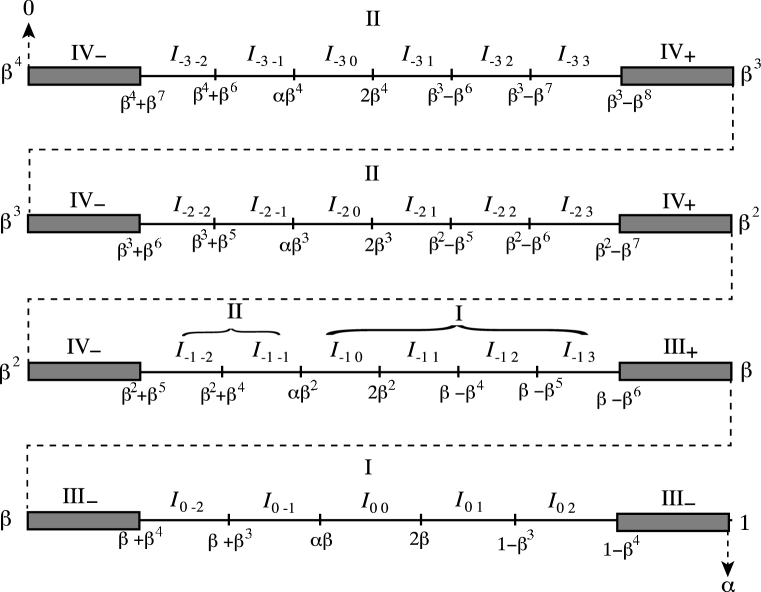
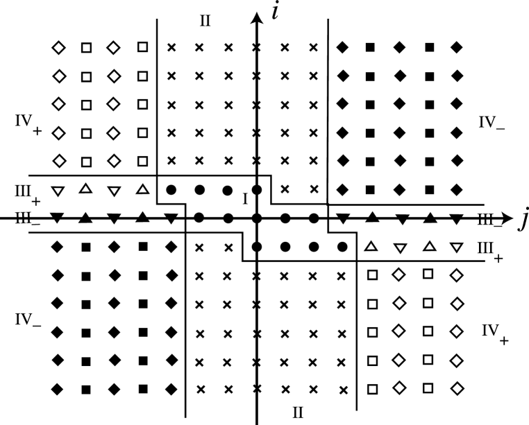
Figure 9 emphasizes the organisation of the ten scenarios on the s𝑠s-axis. Specifically, we display the sub-intervals Ii,jsubscript𝐼𝑖𝑗I_{i,j} and their assignment to the scenarios I–IV for β4s1superscript𝛽4𝑠1\beta^{4}\leqslant s\leqslant 1. The same information is illustrated in figure 10 on the (i,j)𝑖𝑗(i,j)-lattice. Here the labels I–IV denote subsets of 2superscript2\mathbb{Z}^{2}, with suitable added points at infinity. We see that scenario I is restricted to pairs (i,j)𝑖𝑗(i,j) where both indices are small, plus four points at infinity corresponding to s=α,0𝑠𝛼0s=\alpha,0 and s=β,1𝑠𝛽1s=\beta,1, respectively. Scenario II corresponds to small values of j𝑗j, with unbounded i𝑖i (corresponding to s𝑠s approaching 0,α0𝛼0,\alpha), plus a sequence of points at infinity corresponding to the accumulation points β|i|+1superscript𝛽𝑖1\beta^{|i|+1} and αβ|i|+1𝛼superscript𝛽𝑖1\alpha-\beta^{|i|+1}, for |i|1𝑖1|i|\geqslant 1. Scenario III features small values of i𝑖i and unbounded j𝑗j (corresponding to s𝑠s tending to an accumulation point). Finally, scenario IV covers the doubly asymptotic cases. With reference to table 2, we shall use the short-hand notation:

III=μ,νIIIμνIV=μ,νIVμν.IIIsubscript𝜇𝜈subscriptIII𝜇𝜈IVsubscript𝜇𝜈subscriptIV𝜇𝜈\mathrm{III}=\bigcup_{\mu,\nu}\mathrm{III}_{\mu\nu}\hskip 30.0pt\mathrm{IV}=\bigcup_{\mu,\nu}\mathrm{IV}_{\mu\nu}. (28)

Our classification scheme leaves open the possibility of more than one realization of each scenario. Thus, even though mirror sub-intervals Ii,jsubscript𝐼𝑖𝑗I_{i,j} and Ii,jsubscript𝐼𝑖𝑗I_{-i,-j} always belong to the same scenario (as evident in the symmetry of Table 2), the difference in their return paths may be sufficient to have distinct temporal scaling properties. This essentially doubles the number of incidence matrices which we need to calculate.

The dynamical architecture of renormalization in the present model bears a strong, if imperfect, resemblance to that of Rauzy [19, 22] to construct renormalizable interval exchange transformations (IETs), i.e., maps on an interval I𝐼I which permute n𝑛n sub-intervals which form a partition of I𝐼I. At the heart of the Rauzy construction is an irreducible graph (Rauzy graph), each vertex of which is a ‘parametric IET’ corresponding to a permutation of n𝑛n symbols and parametrized by a positive n𝑛n-vector 𝐬𝐬\mathbf{s} of interval lengths. The IET’s of the graph are known as a Rauzy class. Each vertex has two outgoing edges, corresponding to two possible induced return maps, and is associated with a matrix transformation in parameter space, 𝐬𝐫i𝐬,i=0,1formulae-sequencemaps-to𝐬subscript𝐫𝑖𝐬𝑖01\mathbf{s}\mapsto\mathbf{r}_{i}\cdot\mathbf{s},\;i=0,1. To search for strictly renormalizable IET’s, one considers the closed loops of the Rauzy graph, multiplying the 𝐫isubscript𝐫𝑖\mathbf{r}_{i} matrices around a loop and seeking a positive eigenvector of the product matrix.

In the present work, our strategy for proving renormalizability is clearly analogous to Rauzy’s, but of course there are important differences. In particular, our ‘Rauzy class’ of base triangles, pencils, fringed triangles, and double strips is a more variegated collection of parametric dressed domains, with bifurcating parameter dependence and no uniform rules of induction to compare with Rauzy’s. Nevertheless, the general strategy (also applied in the context of polygon-exchange transformations by Schwartz [21]) is the same.
Refer to caption
Figure 9: Portion of the s𝑠s-axis, folded, with distorted scale. The large-|j|𝑗|j| asymptotic regime (scenarios III and IV) is represented by thick segments surrounding the accumulation points βk,k=1,2,3,4formulae-sequencesuperscript𝛽𝑘𝑘1234\beta^{k},\;k=1,2,3,4. The large-|i|𝑖|i| regime (scenarios II and IV) consists of the entire interval [0,αβ2]0𝛼superscript𝛽2[0,\alpha\beta^{2}].
Refer to caption
Figure 10: The ten renormalization scenarios for the indices (i,j)2𝑖𝑗superscript2(i,j)\in\mathbb{Z}^{2}. We write ±plus-or-minus\pm for ±1plus-or-minus1\pm 1. The labels III±subscriptIIIplus-or-minus{\rm III}_{\pm} and IV±subscriptIVplus-or-minus{\rm IV}_{\pm} stand for III±III±+subscriptIIIplus-or-minusabsentsubscriptIIIplus-or-minusabsent{\rm III}_{\pm-}\cup{\rm III}_{\pm+} and IV±IV±+subscriptIVplus-or-minusabsentsubscriptIVplus-or-minusabsent{\rm IV}_{\pm-}\cup{\rm IV}_{\pm+}, respectively. Key: I=,II=×,III++=,III+=,III+=,III=,IV++=,IV+=,IV+=,IV=.formulae-sequenceIformulae-sequenceIIformulae-sequencesubscriptIIIabsentformulae-sequencesubscriptIIIabsentformulae-sequencesubscriptIIIabsentformulae-sequencesubscriptIIIabsentformulae-sequencesubscriptIVabsentformulae-sequencesubscriptIVabsentformulae-sequencesubscriptIVabsentsubscriptIVabsent{\rm I}=\bullet,\;{\rm II}=\times,{\rm III}_{++}=\vartriangle,\;{\rm III}_{+-}=\triangledown,\;{\rm III}_{-+}=\blacktriangle,\;{\rm III}_{--}=\blacktriangledown,{\rm IV}_{++}=\square,\;{\rm IV}_{+-}=\diamondsuit,\;{\rm IV}_{-+}=\blacksquare,\;{\rm IV}_{--}=\blacklozenge.

8 Parametric dressed domains with strips

The reader has already been alerted to the fact that certain classes of parametric dressed domains (pencils, fringed triangles, and double strips) play central roles in our renormalization story. We now define these objects. A common feature of all of them is the presence of a special, quasi-one-dimensional sub-tiling which we call the strip.

8.1 The strip

The prototype strip 𝐒^(l,h)^𝐒𝑙\widehat{\bf S}(l,h) is a tiling with a variable number

2J=2logβ(h/l)2𝐽2subscript𝛽𝑙2J=2\lfloor\log_{\beta}(h/l)\rfloor (29)

of tiles, all of which are reflection-symmetric. If we let hh tend monotonically to zero, the strip undergoes a bifurcation every time h/l𝑙h/l assumes a value βk,k=2,3,formulae-sequencesuperscript𝛽𝑘𝑘23\beta^{k},\;k=2,3,\ldots. The number of tiles increases by two, with the additional tiles being born at one of the vertices at x=h𝑥x=-h. The precise structure of 𝐒^(l,h)^𝐒𝑙\widehat{\bf S}(l,h) is specified in table 3, and illustrated, for J=4𝐽4J=4, in figure 11.

Refer to caption
Figure 11: A strip with 8 tiles.
Table 3: Tiling table of the prototype strip 𝐒^(l,h)^𝐒𝑙\widehat{\bf{S}}(l,h). The origin of coordinates lies on the mid-line of the strip, at distance hh to the right of its vertical edge.
Source PolygonPlacementTileQ#Parameters𝚁#TranslationS^12α(lh),2h0(αl+βh,h)S^14βlβh,βlωh0(l,0)S^23h7(αβl,0)S^2j12jJ24βjlβh,βjlωh4j even0j odd(βj1l,(1)j1(βjlαh))S^2j2jJ23h0j even7j odd(αβjl,0)S^2J31βJ1lβh0J even4J odd(βJ2l,(1)J(βJ1lαh))S^2J28αβJ1l+αβh,2h1J even6J odd(αβJ1lβh,(1)J1h)S^2J11βJlβh4J even0J odd(βJ1l,(1)J1(βJlαh))S^2J7αβJ1lαh3J even6J odd(h,(1)J1(αβJ1lωh)))\begin{array}[]{|c|c|c|c|c|}\hline\cr\vrule\lx@intercol\hfil\mbox{Source Polygon}\hfil\lx@intercol\vrule\lx@intercol&\vrule\lx@intercol\hfil\mbox{Placement}\hfil\lx@intercol\vrule\lx@intercol\\ \hline\cr\mbox{Tile}&Q_{\#}&\mbox{Parameters}&{\tt R}_{\#}&\mbox{Translation}\\ \hline\cr\hline\cr\widehat{\rm S}&12&\alpha(l-h),2h&0&(-\alpha l+\beta h,-h)\\ \hline\cr\hline\cr\widehat{S}_{1}&4&\beta l-\beta h,\beta l-\omega h&0&(-l,0)\\ \hline\cr\widehat{S}_{2}&3&h&7&(-\alpha\beta l,0)\\ \hline\cr\begin{array}[]{c}\widehat{S}_{2j-1}\\ {}_{2\leqslant j\leqslant J-2}\end{array}&4&\beta^{j}l-\beta h,\beta^{j}l-\omega h&\begin{array}[]{cc}4&j\mbox{ even}\\ 0&j\mbox{ odd}\end{array}&(-\beta^{j-1}l,(-1)^{j-1}(\beta^{j}l-\alpha h))\\ \hline\cr\begin{array}[]{c}\widehat{S}_{2j}\\ {}_{2\leqslant j\leqslant J-2}\end{array}&3&h&\begin{array}[]{cc}0&j\mbox{ even}\\ 7&j\mbox{ odd}\end{array}&(-\alpha\beta^{j}l,0)\\ \hline\cr\widehat{S}_{2J-3}&1&\beta^{J-1}l-\beta h&\begin{array}[]{cc}0&J\mbox{ even}\\ 4&J\mbox{ odd}\end{array}&(-\beta^{J-2}l,(-1)^{J}(\beta^{J-1}l-\alpha h))\\ \hline\cr\widehat{S}_{2J-2}&8&-\alpha\beta^{J-1}l+\alpha\beta h,2h&\begin{array}[]{cc}1&J\mbox{ even}\\ 6&J\mbox{ odd}\end{array}&(-\alpha\beta^{J-1}l-\beta h,(-1)^{J-1}h)\\ \hline\cr\widehat{S}_{2J-1}&1&\beta^{J}l-\beta h&\begin{array}[]{cc}4&J\mbox{ even}\\ 0&J\mbox{ odd}\end{array}&(-\beta^{J-1}l,(-1)^{J-1}(\beta^{J}l-\alpha h))\\ \hline\cr\widehat{S}_{2J}&7&\alpha\beta^{J-1}l-\alpha h&\begin{array}[]{cc}3&J\mbox{ even}\\ 6&J\mbox{ odd}\end{array}&(-h,(-1)^{J-1}(\alpha\beta^{J-1}l-\omega h)))\\ \hline\cr\end{array}

8.2 The pencil

The prototype pencil 𝒫^(l,h)^𝒫𝑙\widehat{{\mathcal{P}}}(l,h) is a parametric dressed pentagon with a variable number

2L+1=4+logβ(hl)2𝐿14subscript𝛽𝑙2L+1=4+\lfloor\log_{\beta}(\frac{h}{l})\rfloor

of atoms. Its tiling 𝐏^^𝐏\widehat{\mathbf{P}} is the union of five individual tiles and a strip, namely

𝐏^=P0P1P2P3P4𝚄0𝐒^(βl,h),^𝐏subscript𝑃0subscript𝑃1subscript𝑃2subscript𝑃3subscript𝑃4subscript𝚄0^𝐒𝛽𝑙\widehat{\bf P}=P_{0}\cup P_{1}\cup P_{2}\cup P_{3}\cup P_{4}\cup{\tt U}_{0}\widehat{\bf S}(\beta l,h),

Here we assume a coordinate system aligned with the axis of the pencil and with origin at the centre of the square tile P^0subscript^𝑃0\widehat{P}_{0}. Explicitly, arranging the tiles, apart from P^0subscript^𝑃0\widehat{P}_{0}, in left-to-right order of their anchor points, we have

P^0subscript^𝑃0\displaystyle\widehat{P}_{0} =\displaystyle= Q2(h)subscript𝑄2\displaystyle Q_{2}(h)
P^1subscript^𝑃1\displaystyle\widehat{P}_{1} =\displaystyle= 𝚃(l,0)Q9(βl/αh,h),subscript𝚃𝑙0subscript𝑄9𝛽𝑙𝛼\displaystyle{\tt T}_{(-l,0)}\,Q_{9}(\beta l/\alpha-h,h),
P^2subscript^𝑃2\displaystyle\widehat{P}_{2} =\displaystyle= 𝚃(αβlωh,h)𝚁1Q7(αh),subscript𝚃𝛼𝛽𝑙𝜔subscript𝚁1subscript𝑄7𝛼\displaystyle{\tt T}_{(-\alpha\beta l-\omega h,-h)}\,{\tt R}_{1}\,Q_{7}(\alpha h),
P^3subscript^𝑃3\displaystyle\widehat{P}_{3} =\displaystyle= 𝚃(αβlh,h)𝚁3Q1(βh),subscript𝚃𝛼𝛽𝑙subscript𝚁3subscript𝑄1𝛽\displaystyle{\tt T}_{(-\alpha\beta l-h,-h)}\,{\tt R}_{3}\,Q_{1}(\beta h),
P^4subscript^𝑃4\displaystyle\widehat{P}_{4} =\displaystyle= 𝚃(αβl,0)𝚁7Q3(h),subscript𝚃𝛼𝛽𝑙0subscript𝚁7subscript𝑄3\displaystyle{\tt T}_{(-\alpha\beta l,0)}\,{\tt R}_{7}\,Q_{3}(h),
P^k+4subscript^𝑃𝑘4\displaystyle\widehat{P}_{k+4} =\displaystyle= 𝚄0Sk(βl,h),k=1,,2L4.formulae-sequencesubscript𝚄0subscript𝑆𝑘𝛽𝑙𝑘12𝐿4\displaystyle{\tt U}_{0}\,S_{k}(\beta l,h),\;k=1,\ldots,2L-4.

The span of the tiling is

P^=span(𝐏^)=𝚃(αl+αh,0)Q6(αlωh,h).^Pspan^𝐏subscript𝚃𝛼𝑙𝛼0subscript𝑄6𝛼𝑙𝜔\widehat{\rm P}={\rm span}(\widehat{\bf P})={\tt T}_{(-\alpha l+\alpha h,0)}\,Q_{6}(\alpha l-\omega h,h).

The structure of the pencil is illustrated in fig. 12.

Refer to caption
Figure 12: The pencil prototype 𝒫^(l,h)^𝒫𝑙\widehat{{\mathcal{P}}}(l,h) with 2L+12𝐿12L+1 atoms, for L=6𝐿6L=6, together with the two sub-pencils (L=5𝐿5L=5 and L=4𝐿4L=4) obtained by application of the Pencil Shortening Lemma. Each shortening step (i) contracts the parameter l𝑙l by a factor β𝛽\beta, with no change in the parameter hh, (ii) reduces the number of atoms by two, and (iii) reverses the parity. The nine-atom pencil at the bottom cannot be shortened further without violating the definition of a pencil.

The domain map ρ𝒫^subscript𝜌superscript^𝒫absent\rho_{\stackrel{{\scriptstyle}}{{\widehat{{\mathcal{P}}}}}} for the pencil is defined in terms of a composition of involutions, 𝚄0𝙷subscript𝚄0𝙷{\tt U}_{0}\circ{\tt H}, where 𝙷𝙷{\tt H} is a simultaneous reflection of each tile about an assigned axis. The trapezia, triangles, kites, and the hexagon P^2L2subscript^𝑃2𝐿2\widehat{P}_{2L-2} have a unique reflection symmetry. For the rhombi, we choose the short diagonal, as in the case of the strip. This leaves the square P^0subscript^𝑃0\widehat{P}_{0} and hexagon P^1subscript^𝑃1\widehat{P}_{1}, for which we assign axes parallel to 𝐮7subscript𝐮7\mathbf{u}_{7} and 𝐮2subscript𝐮2\mathbf{u}_{2}, respectively.

Studying the renormalization of pencils with arbitrarily many atoms is made manageable by the Pencil Shortening Lemma, which relates any pencil to a minimal one with only nine atoms. Note that in specifying the associated incidence matrix, we use as matrix indices the canonical atom labels shown in figure 11. For the sake of transparency, we will adopt this convention for all of our incidence matrices throughout this article.

Pencil Shortening Lemma. Let 𝒫(l,h)=(P(l,h),𝐏(l,h),ρ(l,h))𝒫𝑙P𝑙𝐏𝑙𝜌𝑙{\mathcal{P}}(l,h)=(\mathrm{P}(l,h),{\bf P}(l,h),\rho(l,h)) be a pencil congruent to 𝒫^(l,h)^𝒫𝑙\widehat{{\mathcal{P}}}(l,h), with 2L+12𝐿12L+1 tiles (cf. equation (5)). The return maps induced by ρ(l,h)𝜌𝑙\rho(l,h) on the tiles P(βkl,h),k=1,,L4,formulae-sequencePsuperscript𝛽𝑘𝑙𝑘1𝐿4{\rm P}(\beta^{k}l,h),\;k=1,\ldots,L-4, promote the latter to pencils of parity (1)ksuperscript1𝑘(-1)^{k} congruent to P^(βkl,h)^𝑃superscript𝛽𝑘𝑙\widehat{P}(\beta^{k}l,h). For a given L𝐿L, the minimal pencil induced by this shortening process has nine atoms, parity (1)Lsuperscript1𝐿(-1)^{L}, and an incidence matrix (with respect to 𝒫(l,h)𝒫𝑙{\mathcal{P}}(l,h)) given, for i=0,,2L+1𝑖02𝐿1i=0,\ldots,2L+1, by (we label the rows and columns of MM\mathrm{M} by the canonical tile names 𝒫𝒫{\mathcal{P}} and 𝒫superscript𝒫{\mathcal{P}}^{*}, respectively)

MPi,P0subscriptMsubscript𝑃𝑖subscriptsuperscript𝑃0\displaystyle{\rm M}_{P_{i},P^{*}_{0}} =\displaystyle= δi,0,subscript𝛿𝑖0\displaystyle\delta_{i,0},
MPi,P1subscriptMsubscript𝑃𝑖subscriptsuperscript𝑃1\displaystyle{\rm M}_{P_{i},P^{*}_{1}} =\displaystyle= δi,2L5,subscript𝛿𝑖2𝐿5\displaystyle\delta_{i,2L-5},
MPi,P2subscriptMsubscript𝑃𝑖subscriptsuperscript𝑃2\displaystyle{\rm M}_{P_{i},P^{*}_{2}} =\displaystyle= δi,2+2j=42L5δi,j,subscript𝛿𝑖22superscriptsubscript𝑗42𝐿5subscript𝛿𝑖𝑗\displaystyle\delta_{i,2}+2\sum_{j=4}^{2L-5}\delta_{i,j}, (30)
MPi,P3subscriptMsubscript𝑃𝑖subscriptsuperscript𝑃3\displaystyle{\rm M}_{P_{i},P^{*}_{3}} =\displaystyle= 2(δi,2L6+δi,2L5),2subscript𝛿𝑖2𝐿6subscript𝛿𝑖2𝐿5\displaystyle 2(\delta_{i,2L-6}+\delta_{i,2L-5}),
MPi,PjsubscriptMsubscript𝑃𝑖subscriptsuperscript𝑃𝑗\displaystyle{\rm M}_{P_{i},P^{*}_{j}} =\displaystyle= δi,j+2L8, 4j8.subscript𝛿𝑖𝑗2𝐿84𝑗8\displaystyle\delta_{i,j+2L-8},\;4\leqslant j\leqslant 8.

The polygon P(l,h)P𝑙\mathrm{P}(l,h) is tiled, up to a set of zero measure, by the return orbits of the tiles of the minimal pencil, as well as a finite number of periodic tiles.

Proof. Without loss of generality we assume 𝒫(l,h)=𝒫^(l,h)𝒫𝑙^𝒫𝑙{\mathcal{P}}(l,h)=\widehat{{\mathcal{P}}}(l,h). We wish to show that the piecewise isometries ρ(k)superscript𝜌𝑘\rho^{(k)} of the shortened pencils 𝒫(k)=𝚄0k𝒫(βkl,h)superscript𝒫𝑘superscriptsubscript𝚄0𝑘𝒫superscript𝛽𝑘𝑙{\mathcal{P}}^{(k)}={\tt U}_{0}^{k}{\mathcal{P}}(\beta^{k}l,h) are induced return maps of ρ(0)=ρ(l,h)superscript𝜌0𝜌𝑙\rho^{(0)}=\rho(l,h). It suffices to prove it for k=1𝑘1k=1, since the step can be repeated until the pencil is minimal. The proof is by direct iteration of ρ(0)superscript𝜌0\rho^{(0)} on the tiles of 𝒫(1)superscript𝒫1{\mathcal{P}}^{(1)}. Only a small number of tiles have non-trivial return orbits. To see this, we refer to figure 12. All of the tiles in the strip 𝐒(β2l,h)𝐒superscript𝛽2𝑙{\bf S}(\beta^{2}l,h) are mapped the same by ρ(0)superscript𝜌0\rho^{(0)} and by ρ(1)superscript𝜌1\rho^{(1)}. The same is true of P0(1)subscriptsuperscript𝑃10P^{(1)}_{0} and P4(1)subscriptsuperscript𝑃14P^{(1)}_{4}, and even P1(1)subscriptsuperscript𝑃11P^{(1)}_{1}. The remaining tiles, P2(1)subscriptsuperscript𝑃12P^{(1)}_{2} and P3(1)subscriptsuperscript𝑃13P^{(1)}_{3}, have short return orbits which we calculate explicitly: we find that they pass through, in order, P5,P4,P4,P5subscript𝑃5subscript𝑃4subscript𝑃4subscript𝑃5P_{5},P_{4},P_{4},P_{5} and P5,P4,P2,P4,P5subscript𝑃5subscript𝑃4subscript𝑃2subscript𝑃4subscript𝑃5P_{5},P_{4},P_{2},P_{4},P_{5}, respectively.

From the structure of the return orbits, we can write down immediately the incidence matrix for the recursive step from L𝐿L to L1𝐿1L-1. We label the rows and columns of the incidence matrix by the canonical tile names of PP\mathrm{P}:

MPi(0),P0(1)subscriptMsubscriptsuperscript𝑃0𝑖subscriptsuperscript𝑃10\displaystyle{\rm M}_{P^{(0)}_{i},P^{(1)}_{0}} =\displaystyle= δi,0,subscript𝛿𝑖0\displaystyle\delta_{i,0},
MPi(0),P1(1)subscriptMsubscriptsuperscript𝑃0𝑖subscriptsuperscript𝑃11\displaystyle{\rm M}_{P^{(0)}_{i},P^{(1)}_{1}} =\displaystyle= δi,5,subscript𝛿𝑖5\displaystyle\delta_{i,5},
MPi(0),P2(1)subscriptMsubscriptsuperscript𝑃0𝑖subscriptsuperscript𝑃12\displaystyle{\rm M}_{P^{(0)}_{i},P^{(1)}_{2}} =\displaystyle= δi,2+2(δi,4+δi,5)subscript𝛿𝑖22subscript𝛿𝑖4subscript𝛿𝑖5\displaystyle\delta_{i,2}+2(\delta_{i,4}+\delta_{i,5}) (31)
MPi(0),P3(1)subscriptMsubscriptsuperscript𝑃0𝑖subscriptsuperscript𝑃13\displaystyle{\rm M}_{P^{(0)}_{i},P^{(1)}_{3}} =\displaystyle= 2(δi,4+δi,5),2subscript𝛿𝑖4subscript𝛿𝑖5\displaystyle 2(\delta_{i,4}+\delta_{i,5}),
MPi(0),Pj(1)subscriptMsubscriptsuperscript𝑃0𝑖subscriptsuperscript𝑃1𝑗\displaystyle{\rm M}_{P^{(0)}_{i},P^{(1)}_{j}} =\displaystyle= δi,j,6i2L,4j2L2,formulae-sequencesubscript𝛿𝑖𝑗6𝑖2𝐿4𝑗2𝐿2\displaystyle\delta_{i,j},\quad 6\leqslant i\leqslant 2L,\quad 4\leqslant j\leqslant 2L-2,

where in the first four equations the index i𝑖i varies over its full range: 0i2L0𝑖2𝐿0\leqslant i\leqslant 2L.

For the full shortening process of L4𝐿4L-4 steps, ending with a minimal pencil, the proof is by mathematical induction on L𝐿L. The starting point is the case L=5𝐿5L=5, where the one-step incidence matrix is given by (31), which coincides with (30). Given formula (30) for a given L𝐿L, we get the incidence matrix for L+1𝐿1L+1 by multiplication on the right by the recursion matrix defined by (31). One readily verifies that this reproduces the general formulae with L𝐿L incremented by one.

To prove the completeness of the tiling, it is again sufficient to restrict ourselves to a single shortening step. The periodic cells are readily identified cells: the hexagonal period-1 atom P1subscript𝑃1P_{1}, the triangular period-3 atom P3subscript𝑃3P_{3}, and an octagonal period-1 tile inscribed in the rhombic atom P4subscript𝑃4P_{4}. We explicitly verify that the total area of all return orbits is equal to that of the original pencil. That the minimal pencil has 9 atoms follows from the definition of a pencil, while the parity of (1)Lsuperscript1𝐿(-1)^{L} is a consequence of the fact that each of the L4𝐿4L-4 shortening steps is accompanied by a reflection 𝚄0subscript𝚄0{\tt U}_{0}. \Box

8.3 Fringed triangle

There are two prototype fringed triangles 𝒯^±(l,h)subscript^𝒯plus-or-minus𝑙\widehat{\mathcal{T}}_{\pm}(l,h), each containing a strip congruent to 𝐒^(l,h)^𝐒𝑙\widehat{\bf S}(l,h) with a variable number 2J2𝐽2J of atoms. The total numbers of atoms are 2J+22𝐽22J+2 for 𝒯^(l,h)subscript^𝒯𝑙\widehat{{\mathcal{T}}}_{-}(l,h) and 2J+72𝐽72J+7 for 𝒯^(l,h)subscript^𝒯𝑙\widehat{{\mathcal{T}}}_{-}(l,h).

Refer to caption
Figure 13: Tiling of the prototypes 𝒯^±(l,h)subscript^𝒯plus-or-minus𝑙\widehat{{\mathcal{T}}}_{\pm}(l,h).

We begin with 𝒯^(l,h)subscript^𝒯𝑙\widehat{{\mathcal{T}}}_{-}(l,h). Its tiling 𝐓^subscript^𝐓\widehat{\bf T}_{-} is a union of two individual tiles with a strip, namely (see figure 13)

𝐓^=T^1T^2𝚁2𝐒(l,h).subscript^𝐓subscriptsuperscript^𝑇1subscriptsuperscript^𝑇2subscript𝚁2𝐒𝑙\widehat{\bf T}_{-}=\widehat{T}^{-}_{1}\cup\widehat{T}^{-}_{2}\cup{\tt R}_{2}\,{\bf S}(l,h).

Here we assume a coordinate system whose origin coincides with that of the strip, with the mid-line of the strip lined up along the negative y𝑦y-axis. Explicitly,

T^1subscriptsuperscript^𝑇1\displaystyle\widehat{T}^{-}_{1} =\displaystyle= 𝚃(h,h)𝚁5Q1(βl+βh),subscript𝚃subscript𝚁5subscript𝑄1𝛽𝑙𝛽\displaystyle{\tt T}_{(h,-h)}\,{\tt R}_{5}\,Q_{1}(\beta l+\beta h),
T^2subscriptsuperscript^𝑇2\displaystyle\widehat{T}^{-}_{2} =\displaystyle= 𝚃(h,αl+ωh)𝚁3Q7(αlαωh),subscript𝚃𝛼𝑙𝜔subscript𝚁3subscript𝑄7𝛼𝑙𝛼𝜔\displaystyle{\tt T}_{(-h,-\alpha l+\omega h)}\,{\tt R}_{3}\,Q_{7}(\alpha l-\alpha\omega h),
T^k+2subscriptsuperscript^𝑇𝑘2\displaystyle\widehat{T}^{-}_{k+2} =\displaystyle= 𝚁2Sk(l,h),k=1,,2J.formulae-sequencesubscript𝚁2subscript𝑆𝑘𝑙𝑘12𝐽\displaystyle{\tt R}_{2}\,S_{k}(l,h),\;k=1,\ldots,2J.

The span of the tiling is

T^=span(𝐓^)=𝚃(l+αh,βl)𝚁2Q1(lβh).subscript^Tspansubscript^𝐓subscript𝚃𝑙𝛼𝛽𝑙subscript𝚁2subscript𝑄1𝑙𝛽\widehat{\rm T}_{-}={\rm span}(\widehat{\bf T}_{-})={\tt T}_{(-l+\alpha h,-\beta l)}\,{\tt R}_{2}\,Q_{1}(l-\beta h).

Next we turn to the prototype fringed triangle 𝒯^+(l,h)subscript^𝒯𝑙\widehat{{\mathcal{T}}}_{+}(l,h). Its tiling is the union of seven individual tiles and a strip, namely (see figure 13)

𝐓^+=k=17T^k+𝚁3𝐒^(l,h).subscript^𝐓superscriptsubscript𝑘17subscriptsuperscript^𝑇𝑘subscript𝚁3^𝐒𝑙\widehat{\bf T}_{+}=\bigcup_{k=1}^{7}\widehat{T}^{+}_{k}\cup{\tt R}_{3}\,\widehat{\bf S}(l,h).

Here we assume a coordinate system whose origin coincides with that of the strip, with the mid-line of the strip lined up along the negative y𝑦y-axis. Explicitly,

T^1+subscriptsuperscript^𝑇1\displaystyle\widehat{T}^{+}_{1} =\displaystyle= 𝚃((3+α)lh,(1+2α)l+h))𝚁5Q1(ωlβh),\displaystyle{\tt T}_{((3+\alpha)l-h,(1+2\alpha)l+h))}\,{\tt R}_{5}\,Q_{1}(\omega l-\beta h),
T^2+subscriptsuperscript^𝑇2\displaystyle\widehat{T}^{+}_{2} =\displaystyle= 𝚃((3+α)lh,(3+α)l+ωh)𝚁3Q7(αω2lαh),subscript𝚃3𝛼𝑙3𝛼𝑙𝜔subscript𝚁3subscript𝑄7𝛼superscript𝜔2𝑙𝛼\displaystyle{\tt T}_{((3+\alpha)l-h,-(3+\alpha)l+\omega h)}\,{\tt R}_{3}\,Q_{7}(\alpha\omega^{2}l-\alpha h),
T^3+subscriptsuperscript^𝑇3\displaystyle\widehat{T}^{+}_{3} =\displaystyle= 𝚃(αl,αl)𝚁7Q2(h),subscript𝚃𝛼𝑙𝛼𝑙subscript𝚁7subscript𝑄2\displaystyle{\tt T}_{(-\alpha l,\alpha l)}\,{\tt R}_{7}\,Q_{2}(h),
T^4+subscriptsuperscript^𝑇4\displaystyle\widehat{T}^{+}_{4} =\displaystyle= 𝚃(l/α,l/α)𝚁7Q10(h,lh),subscript𝚃𝑙𝛼𝑙𝛼subscript𝚁7subscript𝑄10𝑙\displaystyle{\tt T}_{(-l/\alpha,l/\alpha)}\,{\tt R}_{7}\,Q_{10}(h,l-h),
T^5+subscriptsuperscript^𝑇5\displaystyle\widehat{T}^{+}_{5} =\displaystyle= 𝚁7Q2(h),subscript𝚁7subscript𝑄2\displaystyle{\tt R}_{7}\,Q_{2}(h),
T^6+subscriptsuperscript^𝑇6\displaystyle\widehat{T}^{+}_{6} =\displaystyle= 𝚃((3+α)lh,lh)𝚁7Q4(ωlβh,ωlωh),subscript𝚃3𝛼𝑙𝑙subscript𝚁7subscript𝑄4𝜔𝑙𝛽𝜔𝑙𝜔\displaystyle{\tt T}_{((3+\alpha)l-h,-l-h)}\,{\tt R}_{7}\,Q_{4}(\omega l-\beta h,\omega l-\omega h),
T^7+subscriptsuperscript^𝑇7\displaystyle\widehat{T}^{+}_{7} =\displaystyle= 𝚃(l,l)𝚁7Q3(h),subscript𝚃𝑙𝑙subscript𝚁7subscript𝑄3\displaystyle{\tt T}_{(l,-l)}\,{\tt R}_{7}\,Q_{3}(h),
T^k+7+subscriptsuperscript^𝑇𝑘7\displaystyle\widehat{T}^{+}_{k+7} =\displaystyle= 𝚁3Sk(l,h),k=1,,2J.formulae-sequencesubscript𝚁3subscript𝑆𝑘𝑙𝑘12𝐽\displaystyle{\tt R}_{3}\,S_{k}(l,h),\;k=1,\ldots,2J.

The span of the tiling is

T^+=span(𝐓^+)=𝚃(αl+αh,αl)𝚁2Q1(ω2l+βh).subscript^Tspansubscript^𝐓subscript𝚃𝛼𝑙𝛼𝛼𝑙subscript𝚁2subscript𝑄1superscript𝜔2𝑙𝛽\widehat{\rm T}_{+}={\rm span}(\widehat{\bf T}_{+})={\tt T}_{(-\alpha l+\alpha h,\alpha l)}\,{\tt R}_{2}\,Q_{1}(\omega^{2}l+\beta h).

The domain maps ρ𝒯±±subscript𝜌superscriptsubscript𝒯plus-or-minusabsent\rho_{\stackrel{{\scriptstyle}}{{{\mathcal{T}}_{\pm}}}} of the fringed triangles are defined in terms of a composition of involutions, namely a simultaneous reflection of each atom about an assigned axis, followed by a reflection about the triangle’s symmetry axis. As in the case of the pencil, the assigned axis of each rhombic atom is its short diagonal. For the atoms T^3+subscriptsuperscript^𝑇3\widehat{T}^{+}_{3}, T^4+subscriptsuperscript^𝑇4\widehat{T}^{+}_{4}, and T^5+subscriptsuperscript^𝑇5\widehat{T}^{+}_{5}, the assigned axes are parallel to 𝐮2,𝐮3subscript𝐮2subscript𝐮3\mathbf{u}_{2},\mathbf{u}_{3}, and 𝐮2subscript𝐮2\mathbf{u}_{2}, respectively.

8.4 Double strip

The prototype double strip 𝒟^ν(l,h),ν=±1,subscript^𝒟𝜈𝑙𝜈plus-or-minus1\widehat{{\mathcal{D}}}_{\nu}(l,h),\;\nu=\pm 1, is a dressed domain constructed out of a square and two strips, one on the left with positive parity and 2K2𝐾2K atoms, the other on the right with negative parity and 2K22𝐾22K-2 atoms. Since a well-defined strip has at least four tiles, a double strip requires at least 11 atoms (i.e., K3𝐾3K\geqslant 3). For both signs ν𝜈\nu, we define the prototype to have the tiling

𝐃^(l,h)=𝐒(ωl,h)D^0𝚄2𝐒(l,h),D^0=Q2(h).formulae-sequence^𝐃𝑙𝐒𝜔𝑙subscript^𝐷0subscript𝚄2𝐒𝑙subscript^𝐷0subscript𝑄2\widehat{\bf D}(l,h)={\bf S}(\omega l,h)\,\cup\,\widehat{D}_{0}\,\cup{\tt U}_{2}\,{\bf S}(l,h),\hskip 30.0pt\widehat{D}_{0}=Q_{2}(h).

Note the appearance of the reflection operator 𝚄2subscript𝚄2{\tt U}_{2} to correctly place and orient one of the component strips. A prototype double strip is illustrated in figure 14. Here and in what follows we adopt a canonical labelling of the tiles of any double strip 𝒟𝒟{\mathcal{D}}, in order along the midline,

D1′′,D2′′,,D2K′′,D0,D2K2,,D1,subscriptsuperscript𝐷′′1subscriptsuperscript𝐷′′2subscriptsuperscript𝐷′′2𝐾subscript𝐷0subscriptsuperscript𝐷2𝐾2subscriptsuperscript𝐷1D^{{}^{\prime\prime}}_{1},D^{{}^{\prime\prime}}_{2},\ldots,D^{{}^{\prime\prime}}_{2K},D_{0},D^{{}^{\prime}}_{2K-2},\ldots,D^{{}^{\prime}}_{1},
Refer to caption
Figure 14: Prototype double strip.

The distinction between 𝒟^+(l,h)subscript^𝒟𝑙\widehat{{\mathcal{D}}}_{+}(l,h) and 𝒟^(l,h)subscript^𝒟𝑙\widehat{{\mathcal{D}}}_{-}(l,h) enters when we specify the piecewise isometry ρ𝒟^ννsubscript𝜌superscriptsubscript^𝒟𝜈absent\rho_{\stackrel{{\scriptstyle}}{{\widehat{{\mathcal{D}}}_{\nu}}}}. As before, we define the map as a composition of two involutions, the reflection of each atom about an assigned symmetry axis, followed by reflection about the vertical symmetry axis of the double strip as a whole. Once again the axes of the rhombi are their short diagonals. The square D^0subscript^𝐷0\widehat{D}_{0}, on the other hand, is assigned the diagonal 𝐮1subscript𝐮1\mathbf{u}_{1} for ν=+𝜈\nu=+ and 𝐮3subscript𝐮3\mathbf{u}_{3} for ν=𝜈\nu=-. A considerable simplification of the renormalization structure results from the following ‘shortening’ lemma:

Double-Strip Shortening Lemma. Let 𝒟(l,h)=(D(l,h),𝐃(l,h),ρ(l,h))𝒟𝑙D𝑙𝐃𝑙𝜌𝑙{\mathcal{D}}(l,h)=(\mathrm{D}(l,h),{\bf D}(l,h),\rho(l,h)) be a double strip congruent to 𝒟^ν(l,h)subscript^𝒟𝜈𝑙\widehat{{\mathcal{D}}}_{\nu}(l,h), with 4K14𝐾14K-1 tiles. The return maps induced by ρ(l,h)𝜌𝑙\rho(l,h) on the tiles 𝚄2kD(βkl,h),k=1,,K3,formulae-sequencesuperscriptsubscript𝚄2𝑘Dsuperscript𝛽𝑘𝑙𝑘1𝐾3{\tt U}_{2}^{k}{\rm D}(\beta^{k}l,h),\;k=1,\ldots,K-3, promote the latter to double strips of parity (1)ksuperscript1𝑘(-1)^{k} congruent to D^ν(k)(βkl,h)subscript^𝐷superscript𝜈𝑘superscript𝛽𝑘𝑙\widehat{D}_{\nu^{(k)}}(\beta^{k}l,h), with ν(k)=(1)kνsuperscript𝜈𝑘superscript1𝑘𝜈\nu^{(k)}=(-1)^{k}\nu. For a given K𝐾K, the minimal double strip induced by this shortening process has 11 atoms, parity (1)K3superscript1𝐾3(-1)^{K-3}, index νK3=(1)K3νsubscript𝜈𝐾3superscript1𝐾3𝜈\nu_{K-3}=(-1)^{K-3}\nu, and an incidence matrix (with respect to 𝒟(l,h)𝒟𝑙{\mathcal{D}}(l,h)) given, for K𝐾K odd, by

MD,D0oddsubscriptsuperscriptModd𝐷subscript𝐷0\displaystyle{\rm M}^{\rm odd}_{D,D_{0}} =\displaystyle= δD,D0+NDodd,subscript𝛿𝐷subscript𝐷0superscriptsubscriptN𝐷odd\displaystyle\delta_{D,D_{0}}+{\rm N}_{D}^{\rm odd},
MD,Dk′′oddsubscriptsuperscriptModd𝐷subscriptsuperscript𝐷′′𝑘\displaystyle{\rm M}^{\rm odd}_{D,D^{{}^{\prime\prime}}_{k}} =\displaystyle= δD,D2K+k6′′+NDodd,k=1,,6,formulae-sequencesubscript𝛿𝐷subscriptsuperscript𝐷′′2𝐾𝑘6superscriptsubscriptN𝐷odd𝑘16\displaystyle\delta_{D,D^{{}^{\prime\prime}}_{2K+k-6}}+{\rm N}_{D}^{\rm odd},\quad k=1,\ldots,6, (32)
MD,DkoddsubscriptsuperscriptModd𝐷subscriptsuperscript𝐷𝑘\displaystyle{\rm M}^{\rm odd}_{D,D^{{}^{\prime}}_{k}} =\displaystyle= δD,D2K+k6+NDodd,k=1,4,formulae-sequencesubscript𝛿𝐷subscriptsuperscript𝐷2𝐾𝑘6superscriptsubscriptN𝐷odd𝑘14\displaystyle\delta_{D,D^{{}^{\prime}}_{2K+k-6}}+{\rm N}_{D}^{\rm odd},\quad k=1\ldots,4,
NDodd=k=1K32(24k1δD,D2K4k5′′+4k1δD,D2K4k5),superscriptsubscriptN𝐷oddsuperscriptsubscript𝑘1𝐾322superscript4𝑘1subscript𝛿𝐷subscriptsuperscript𝐷′′2𝐾4𝑘5superscript4𝑘1subscript𝛿𝐷subscriptsuperscript𝐷2𝐾4𝑘5{\rm N}_{D}^{\rm odd}=\sum_{k=1}^{\frac{K-3}{2}}\left(2\cdot 4^{k-1}\,\delta_{D,D^{{}^{\prime\prime}}_{2K-4k-5}}+4^{k-1}\,\delta_{D,D^{{}^{\prime}}_{2K-4k-5}}\right), (33)

and, for K𝐾K even, by

MD,D0evensubscriptsuperscriptMeven𝐷subscript𝐷0\displaystyle{\rm M}^{\rm even}_{D,D_{0}} =\displaystyle= δD,D0+NDeven,subscript𝛿𝐷subscript𝐷0superscriptsubscriptN𝐷even\displaystyle\delta_{D,D_{0}}+{\rm N}_{D}^{\rm even},
MD,Dk′′evensubscriptsuperscriptMeven𝐷subscriptsuperscript𝐷′′𝑘\displaystyle{\rm M}^{\rm even}_{D,D^{{}^{\prime\prime}}_{k}} =\displaystyle= δD,D2K+k8+NDeven,k=1,,6,formulae-sequencesubscript𝛿𝐷subscriptsuperscript𝐷2𝐾𝑘8superscriptsubscriptN𝐷even𝑘16\displaystyle\delta_{D,D^{{}^{\prime}}_{2K+k-8}}+{\rm N}_{D}^{\rm even},\quad k=1,\ldots,6, (34)
MD,DkevensubscriptsuperscriptMeven𝐷subscriptsuperscript𝐷𝑘\displaystyle{\rm M}^{\rm even}_{D,D^{{}^{\prime}}_{k}} =\displaystyle= δD,D2K+k4′′+NDeven,k=1,,4,formulae-sequencesubscript𝛿𝐷subscriptsuperscript𝐷′′2𝐾𝑘4superscriptsubscriptN𝐷even𝑘14\displaystyle\delta_{D,D^{{}^{\prime\prime}}_{2K+k-4}}+{\rm N}_{D}^{\rm even},\quad k=1,\ldots,4,
NDeven=k=1K22(24k1δD,D2K4k7+4k1δD,D2K4k3′′),superscriptsubscriptN𝐷evensuperscriptsubscript𝑘1𝐾222superscript4𝑘1subscript𝛿𝐷subscriptsuperscript𝐷2𝐾4𝑘7superscript4𝑘1subscript𝛿𝐷subscriptsuperscript𝐷′′2𝐾4𝑘3{\rm N}_{D}^{\rm even}=\sum_{k=1}^{\frac{K-2}{2}}\left(2\cdot 4^{k-1}\,\delta_{D,D^{{}^{\prime}}_{2K-4k-7}}+4^{k-1}\,\delta_{D,D^{{}^{\prime\prime}}_{2K-4k-3}}\right), (35)

where the subscript D𝐷D denotes an arbitrary element of 𝐃(l,h)𝐃𝑙\mathbf{D}(l,h).

The polygon D(l,h)D𝑙{\rm D}(l,h) is tiled, up to a set of zero measure, by the return orbits of the tiles of the minimal double strip, as well as a finite number of periodic cells.

Proof. To show that the piecewise isometries ρ(k)superscript𝜌𝑘\rho^{(k)} of the shortened double strips 𝒟(k)=𝚄2k𝒟νk(βkl,h)superscript𝒟𝑘superscriptsubscript𝚄2𝑘subscript𝒟subscript𝜈𝑘superscript𝛽𝑘𝑙{\mathcal{D}}^{(k)}={\tt U}_{2}^{k}{\mathcal{D}}_{\nu_{k}}(\beta^{k}l,h) are induced return maps of ρ(0)=ρ(l,h)superscript𝜌0𝜌𝑙\rho^{(0)}=\rho(l,h), it suffices to prove it for k=1𝑘1k=1, since this step can be repeated until the double strip is minimal. Here we utilize the decomposition of each ρ(k)superscript𝜌𝑘\rho^{(k)} into a product of involutions, ρ(k)=𝚄(k)𝙷(k),k=0,1,formulae-sequencesuperscript𝜌𝑘superscript𝚄𝑘superscript𝙷𝑘𝑘01\rho^{(k)}={\tt U}^{(k)}{\tt H}^{(k)},k=0,1, where 𝙷(k)superscript𝙷𝑘{\tt H}^{(k)} reflects each tile about its own specified symmetry axis, while 𝚄(k)superscript𝚄𝑘{\tt U}^{(k)} is a global reflection about the symmetry axis of 𝒟(k)superscript𝒟𝑘{\mathcal{D}}^{(k)} as a whole.

A key observation is that the tiles of 𝒟(1)superscript𝒟1{\mathcal{D}}^{(1)} coincide with the 4K54𝐾54K-5 rightmost tiles of 𝒟(0)superscript𝒟0{\mathcal{D}}^{(0)}, and the span of these tiles, D(1)superscriptD1{\rm D}^{(1)}, is mapped by a single application of ρ(0)superscript𝜌0\rho^{(0)} onto D1(0)′′subscriptsuperscript𝐷superscript0′′1D^{(0)^{\prime\prime}}_{1}, the leftmost (and largest) tile of 𝒟(0)superscript𝒟0{\mathcal{D}}^{(0)}. Under the global reflection 𝚄(0)superscript𝚄0{\tt U}^{(0)}, these two trapezoids are reflected about their respective symmetry axes and interchanged. One important consequence is the identity (for points of D(1)superscriptD1{\rm D}^{(1)}),

𝚄(1)=𝚄(0)𝙷(0)𝚄(0).superscript𝚄1superscript𝚄0superscript𝙷0superscript𝚄0{\tt U}^{(1)}={\tt U}^{(0)}{\tt H}^{(0)}{\tt U}^{(0)}. (36)

Two iterations of ρ(0)=𝚄(0)𝙷(0)superscript𝜌0superscript𝚄0superscript𝙷0\rho^{(0)}={\tt U}^{(0)}{\tt H}^{(0)} map a point of D(1)superscriptD1{\rm D}^{(1)} back into that polygon for the first time, hence constitute the first-return map induced by ρ(0)superscript𝜌0\rho^{(0)}. We must still show that ρ(0)2=ρ(1)superscript𝜌02superscript𝜌1\rho^{(0)2}=\rho^{(1)} on D(1)superscriptD1{\rm D}^{(1)}. But this follows from

ρ(0)2=𝚄(0)𝙷(0)𝚄(0)𝙷(0)=𝚄(1)𝙷(1),superscript𝜌02superscript𝚄0superscript𝙷0superscript𝚄0superscript𝙷0superscript𝚄1superscript𝙷1\rho^{(0)2}={\tt U}^{(0)}{\tt H}^{(0)}{\tt U}^{(0)}{\tt H}^{(0)}={\tt U}^{(1)}{\tt H}^{(1)},

where we have used (36) and the fact that 𝙷(0)superscript𝙷0{\tt H}^{(0)} and 𝙷(1)superscript𝙷1{\tt H}^{(1)} coincide on D(1)superscriptD1{\rm D}^{(1)}. The opposite signs of ν(0)superscript𝜈0\nu^{(0)} and ν(1)superscript𝜈1\nu^{(1)} are crucial here to maintain a consistent symmetry axis for the square tile. That the parity of the double strip changes with each shortening step is an obvious concomitant of the action of the reflection operator 𝚄2subscript𝚄2{\tt U}_{2}.

To see the completeness of the tiling, it is again sufficient to restrict ourselves to the single step, from 𝒟(0)superscript𝒟0{\mathcal{D}}^{(0)} to 𝒟(1)superscript𝒟1{\mathcal{D}}^{(1)}. We can focus on those tiles of the former which are not covered by the return orbits of the tiles of the latter. These are precisely Dj(0),j=2,3,4formulae-sequencesubscriptsuperscript𝐷0𝑗𝑗234D^{(0)}_{j},\;j=2,3,4. From the decomposition ρ(0)=𝚄(0)𝙷(0)superscript𝜌0superscript𝚄0superscript𝙷0\rho^{(0)}={\tt U}^{(0)}{\tt H}^{(0)}, it follows that D3(0)subscriptsuperscript𝐷03D^{(0)}_{3}, a trapezoid whose symmetry axis coincides with the global symmetry axis, is a period-1 cell, while the symmetrically deployed rhombi D2(0)subscriptsuperscript𝐷02D^{(0)}_{2} and D4(0)subscriptsuperscript𝐷04D^{(0)}_{4} form a 2-cycle. Thus all points of D(0)superscriptD0{\rm D}^{(0)} are covered, up to boundary points, by the return orbits of 𝒟(1)superscript𝒟1{\mathcal{D}}^{(1)} and the periodic cells just discussed.

Finally we turn to the incidence matrices. From our discussion of the two-step return orbits, we can immediately write down the incidence matrix for the shortening process from a double strip labeled by K𝐾K to the shortened one labeled by K1𝐾1K-1. Here we label the columns of the incidence matrix by the canonical tile names of 𝒟(K1)superscript𝒟𝐾1{\mathcal{D}}^{(K-1)}, while the row index D𝐷D stands for an arbitrary tile label of 𝒟(K)superscript𝒟𝐾{\mathcal{D}}^{(K)}.

MD,D0subscriptM𝐷subscript𝐷0\displaystyle{\rm M}_{D,D_{0}} =\displaystyle= δD,D0+δD,D1′′,subscript𝛿𝐷subscript𝐷0subscript𝛿𝐷superscriptsubscript𝐷1′′\displaystyle\delta_{D,D_{0}}+\delta_{D,D_{1}^{\prime\prime}},
MD,Dk′′subscriptM𝐷superscriptsubscript𝐷𝑘′′\displaystyle{\rm M}_{D,D_{k}^{\prime\prime}} =\displaystyle= δD,Dk+δD,D1′′,k=1,,2K2formulae-sequencesubscript𝛿𝐷superscriptsubscript𝐷𝑘subscript𝛿𝐷superscriptsubscript𝐷1′′𝑘12𝐾2\displaystyle\delta_{D,D_{k}^{\prime}}+\delta_{D,D_{1}^{\prime\prime}},\quad k=1,\ldots,2K-2 (37)
MD,DksubscriptM𝐷superscriptsubscript𝐷𝑘\displaystyle{\rm M}_{D,D_{k}^{\prime}} =\displaystyle= δD,D4+k′′+δD,D1′′,k=1,,2K4.formulae-sequencesubscript𝛿𝐷superscriptsubscript𝐷4𝑘′′subscript𝛿𝐷superscriptsubscript𝐷1′′𝑘12𝐾4\displaystyle\delta_{D,D_{4+k}^{\prime\prime}}+\delta_{D,D_{1}^{\prime\prime}},\quad k=1,\ldots,2K-4.

For the full shortening process of K3𝐾3K-3 steps, ending with a minimal double strip, the proof is by mathematical induction on K𝐾K. The starting point is the case K=4𝐾4K=4, where the one-step incidence matrix is given by (37). Given formulae (32) and (33), or (34) and (35), for a given K𝐾K, we get the incidence matrix for K+1𝐾1K+1 by multiplication on the right by the recursion matrix defined by (37). One readily verifies that this reproduces the general formulae with K𝐾K incremented by one. \Box

9 Arrowheads

In the preceding section we have obtained a detailed description of the dressed domains participating in the renormalization. Together they account for all of the vertices of the renormalization graph. We are now left with the task of establishing the edges. Two of the latter have already been discussed: the inductions 𝒫𝒫𝒫superscript𝒫{\mathcal{P}}\rightarrow{\mathcal{P}}^{*} and 𝒟μ𝒟νsubscript𝒟𝜇subscriptsuperscript𝒟𝜈{\mathcal{D}}_{\mu}\rightarrow{\mathcal{D}}^{*}_{\nu} are implemented by the pencil and double-strip shortening lemmas of the preceding section. Three of the others, namely {\mathcal{B}}\rightarrow{\mathcal{B}}, 𝒫superscript𝒫{\mathcal{P}}^{*}\rightarrow{\mathcal{B}}, and 𝒟νsubscriptsuperscript𝒟𝜈{\mathcal{D}}^{*}_{\nu}\rightarrow{\mathcal{B}}, will be established in the next section by direct iteration of the parent piecewise isometry. As we shall see, the remaining links all involve return-map partitions which produce strips in the child dressed domain, a process which has at its heart the dynamics of a parametric, partially dressed domain, the arrowhead. In the present section we study arrowhead dynamics, establishing an important lemma which will be applied numerous times in the proofs of section 10.

What distinguishes the arrowhead from the parametric dressed domains of the previous section is that its piecewise isometry is left undefined on one of its three tiles. Thus it cannot be viewed as a self-standing dynamical system. As a dressed sub-domain, however, the arrowhead is fully functional, with the missing isometry supplied, via induction, by the PWI of its parent. The flexibility of this arrangement will allow us, in our proof of various renormalization scenarios, to bring to bear the strip-building machinery of the arrowhead in a variety of different contexts.

9.1 Prototype

For h(0,l)0𝑙h\in(0,l), we define the arrowhead prototype as

𝒜^(l,h)=(A,𝐀,ρ𝒜),A=span(𝐀),formulae-sequence^𝒜𝑙A𝐀subscript𝜌superscript𝒜absentAspan𝐀\widehat{{\mathcal{A}}}(l,h)=(\mathrm{A},{\bf A},\rho_{\stackrel{{\scriptstyle}}{{\mathcal{A}}}}),\qquad\mathrm{A}=\mathrm{span}(\mathbf{A}),

where, for 0<h/l<β,𝐀=(A1,A2,A3)formulae-sequence0𝑙𝛽𝐀subscript𝐴1subscript𝐴2subscript𝐴30<h/l<\beta,\;\mathbf{A}=(A_{1},A_{2},A_{3}), with

A1subscript𝐴1\displaystyle A_{1} =\displaystyle= 𝚃(α(lh),0)𝚁2Q1(ω(lh)),subscript𝚃𝛼𝑙0subscript𝚁2subscript𝑄1𝜔𝑙\displaystyle{\tt T}_{(-\alpha(l-h),0)}\,{\tt R}_{2}\,Q_{1}(\omega(l-h)),
A2subscript𝐴2\displaystyle A_{2} =\displaystyle= 𝚃(β(lh),lh)𝚁5Q13(α(lh),2h),subscript𝚃𝛽𝑙𝑙subscript𝚁5subscript𝑄13𝛼𝑙2\displaystyle{\tt T}_{(-\beta(l-h),l-h)}\,{\tt R}_{5}\,Q_{13}(\alpha(l-h),2h),
A3subscript𝐴3\displaystyle A_{3} =\displaystyle= 𝚃(lβh,l+ωh)𝚁4Q1(lωh),subscript𝚃𝑙𝛽𝑙𝜔subscript𝚁4subscript𝑄1𝑙𝜔\displaystyle{\tt T}_{(-l-\beta h,-l+\omega h)}\,{\tt R}_{4}\,Q_{1}(l-\omega h),

and, for βh/l<1,𝐀=(A1,A2)formulae-sequence𝛽𝑙1𝐀subscript𝐴1subscript𝐴2\beta\leqslant h/l<1,\;\mathbf{A}=(A_{1},A_{2}), with

A1subscript𝐴1\displaystyle A_{1} =\displaystyle= 𝚃(α(lh),0)𝚁2Q1(ω(lh)),subscript𝚃𝛼𝑙0subscript𝚁2subscript𝑄1𝜔𝑙\displaystyle{\tt T}_{(-\alpha(l-h),0)}\,{\tt R}_{2}\,Q_{1}(\omega(l-h)),
A2subscript𝐴2\displaystyle A_{2} =\displaystyle= 𝚃(α(lh),0)𝚁4Q1(lh).subscript𝚃𝛼𝑙0subscript𝚁4subscript𝑄1𝑙\displaystyle{\tt T}_{(-\alpha(l-h),0)}{\tt R}_{4}\,Q_{1}(l-h).

The non-convex polygon AA\mathrm{A} is equal to the union of the isosceles right triangle A1subscript𝐴1A_{1} with its reflection about the axis 𝐮52subscript𝐮52\mathbf{u}_{\frac{5}{2}}:

A=A1𝚄52A1.Asubscript𝐴1subscript𝚄52subscript𝐴1{\rm A}=A_{1}\cup{\tt U}_{\frac{5}{2}}A_{1}.

Note that the origin of coordinates (anchor point for the arrowhead) has been taken to be the in-centre of AA{\rm A}, i.e., the centre of an inscribed circle of radius lh𝑙l-h. The piecewise isometry ρ𝒜subscript𝜌superscript𝒜absent\rho_{\stackrel{{\scriptstyle}}{{\mathcal{A}}}} acts on the tiles of 𝐀𝐀{\bf A} as

ρ1=defρ|A1=𝚁5,ρ3=defρ|A3=𝚃(2l,2l)𝚁1,formulae-sequencesuperscriptdefsubscript𝜌1evaluated-at𝜌subscript𝐴1subscript𝚁5superscriptdefsubscript𝜌3evaluated-at𝜌subscript𝐴3subscript𝚃2𝑙2𝑙subscript𝚁1\rho_{1}\stackrel{{\scriptstyle\rm def}}{{=}}\rho|_{A_{1}}={\tt R}_{5},\qquad\rho_{3}\stackrel{{\scriptstyle\rm def}}{{=}}\rho|_{A_{3}}={\tt T}_{(2l,2l)}\,{\tt R}_{1},

with the isometry ρ2subscript𝜌2\rho_{2} on A2subscript𝐴2A_{2} left to be defined by induction in cases where the arrowhead is a dressed sub-domain. Since in all of our applications, the induced map takes A2subscript𝐴2A_{2} outside the arrowhead, we shall refer to the latter as the exit tile. The inverse map is given by

ρ𝒜1=𝚄52ρ𝒜𝚄52.subscriptsuperscript𝜌1superscript𝒜absentsubscript𝚄52subscript𝜌superscript𝒜absentsubscript𝚄52\rho^{-1}_{\stackrel{{\scriptstyle}}{{\mathcal{A}}}}={\tt U}_{\frac{5}{2}}\circ\rho_{\stackrel{{\scriptstyle}}{{\mathcal{A}}}}\circ{\tt U}_{\frac{5}{2}}.

The atoms {A11,A21,A31}superscriptsubscript𝐴11superscriptsubscript𝐴21superscriptsubscript𝐴31\{A_{1}^{-1},A_{2}^{-1},A_{3}^{-1}\} of ρ𝒜1subscriptsuperscript𝜌1superscript𝒜absent\rho^{-1}_{\stackrel{{\scriptstyle}}{{\mathcal{A}}}} are just the reflected images of those of ρ𝒜subscript𝜌superscript𝒜absent\rho_{\stackrel{{\scriptstyle}}{{\mathcal{A}}}}, with ρ𝒜1subscriptsuperscript𝜌1superscript𝒜absent\rho^{-1}_{\stackrel{{\scriptstyle}}{{\mathcal{A}}}} undefined intrinsically on entrance tile A21subscriptsuperscript𝐴12A^{-1}_{2}. The parametrization of the arrowhead 𝒜(l,h)𝒜𝑙{\mathcal{A}}(l,h) and the action of ρ𝒜subscript𝜌superscript𝒜absent\rho_{\stackrel{{\scriptstyle}}{{\mathcal{A}}}} is illustrated in figures 15 and 16.

Refer to caption
Figure 15: The prototype arrowhead 𝒜(l,h)𝒜𝑙{\mathcal{A}}(l,h) and its domain map ρ𝒜subscript𝜌superscript𝒜absent\rho_{\stackrel{{\scriptstyle}}{{{\mathcal{A}}}}}, for 0<h/l<β0𝑙𝛽0<h/l<\beta.
Refer to caption
Figure 16: The prototype arrowhead 𝒜(l,h)𝒜𝑙{\mathcal{A}}(l,h) and its domain map ρ𝒜subscript𝜌superscript𝒜absent\rho_{\stackrel{{\scriptstyle}}{{{\mathcal{A}}}}}, for βh/l<1𝛽𝑙1\beta\leqslant h/l<1.

9.2 Transfer map and the Arrowhead Lemma

For the arrowhead 𝒜^(l,h)^𝒜𝑙\widehat{{\mathcal{A}}}(l,h), we define the transfer map ψ𝜓\psi to be the piecewise isometry induced by ρ𝒜subscript𝜌superscript𝒜absent\rho_{\stackrel{{\scriptstyle}}{{\mathcal{A}}}} mapping the entrance tile A21subscriptsuperscript𝐴12A^{-1}_{2} onto the exit tile A2subscript𝐴2A_{2}. The Arrowhead Lemma below shows that this map is well-defined as a composition of two involutions. In particular, there is a partition of A21subscriptsuperscript𝐴12A^{-1}_{2} into 2J(l,h)=logβ(h/l)2𝐽𝑙subscript𝛽𝑙2J(l,h)=\lfloor\log_{\beta}(h/l)\rfloor tiles, each of which gets mapped isometrically into A2subscript𝐴2A_{2} by iterations of ρ𝒜subscript𝜌superscript𝒜absent\rho_{\stackrel{{\scriptstyle}}{{\mathcal{A}}}}. The area-preserving property of the domain map ensures that the transfer orbits are finite. Figure 17 illustrates the principal features of ψ𝜓\psi in a case where J(l,h)>1𝐽𝑙1J(l,h)>1. In the special case J(l,h)=1𝐽𝑙1J(l,h)=1, which arises for h/l[β,1)𝑙𝛽1h/l\in[\beta,1), the transfer orbits are displayed in figure 18.

Refer to caption
Figure 17: Illustration of statements i)i) and ii)ii) of the Arrowhead Lemma, in an example where the transfer map partition of the entrance tile is a strip with 8 tiles. The point 𝐩𝐩\mathbf{p}, at the intersection of the midlines of the entrance and exit tiles and the arrowhead symmetry axis, plays an important role in the proof of the Arrowhead Lemma.

Arrowhead Lemma. Let 𝒜=𝒜^(l,h)𝒜^𝒜𝑙{\mathcal{A}}=\widehat{{\mathcal{A}}}(l,h), with l>0𝑙0l>0 and h(0,l)0𝑙h\in(0,l). The following holds:

i)i) For h/l(0,β)𝑙0𝛽h/l\in(0,\beta), the tiling 𝐄={E1,,E2J(l,h)}𝐄subscript𝐸1subscript𝐸2𝐽𝑙\mathbf{E}=\{E_{1},\ldots,E_{2J(l,h)}\} of the entrance tile of 𝒜𝒜{\mathcal{A}} by the transfer map ψ𝜓\psi coincides with the strip 𝚃(l,l)𝐒^(l,h)subscript𝚃𝑙𝑙^𝐒𝑙\mathtt{T}_{(l,l)}\widehat{\bf S}(l,h). For h/l[β,1)𝑙𝛽1h/l\in[\beta,1), the tiling 𝐄={E1,,E2}𝐄subscript𝐸1subscript𝐸2\mathbf{E}=\{E_{1},\ldots,E_{2}\} is given in table 4.

ii)ii) The transfer map acts as a composition of two involutions: a simultaneous reflection of the tiles Eisubscript𝐸𝑖E_{i} of the entrance strip about their respective symmetry axes, followed by a reflection about the symmetry axis of 𝒜𝒜{{\mathcal{A}}}. For rhombi, the relevant symmetry axis is the short diagonal.

iii)iii) The incidence matrix column 𝙽(Ej)𝙽subscript𝐸𝑗{\tt N}(E_{j}), listing the number of times the transfer orbit of the entrance strip atom Ejsubscript𝐸𝑗E_{j} visits tiles A1subscript𝐴1A_{1} and A3subscript𝐴3A_{3}, is given by

𝙽(E2k1)𝙽subscript𝐸2𝑘1\displaystyle{\tt N}(E_{2k-1}) =\displaystyle= (12(1)k+323k12+(1)k+123k),12superscript1𝑘32superscript3𝑘12superscript1𝑘12superscript3𝑘\displaystyle\left(\begin{array}[]{c}-\frac{1}{2}-(-1)^{k}+\frac{3}{2}3^{k}\\ -\frac{1}{2}+(-1)^{k}+\frac{1}{2}3^{k}\end{array}\right), (40)
𝙽(E2k)𝙽subscript𝐸2𝑘\displaystyle{\tt N}(E_{2k}) =\displaystyle= (1214(1)k+343k12+14(1)k+143k)1214superscript1𝑘34superscript3𝑘1214superscript1𝑘14superscript3𝑘\displaystyle\left(\begin{array}[]{c}-\frac{1}{2}-\frac{1}{4}(-1)^{k}+\frac{3}{4}3^{k}\\ -\frac{1}{2}+\frac{1}{4}(-1)^{k}+\frac{1}{4}3^{k}\end{array}\right) (44)

with k=1,,J(h,l)𝑘1𝐽𝑙k=1,\ldots,J(h,l).

iv)iv) The orbits of ψ𝜓\psi, including their destination tiles, together with the periodic orbits of the octagonal tiles Π(k)=𝚃γ(k)Q5(βklh),k=0,1,,formulae-sequencesuperscriptΠ𝑘subscript𝚃superscript𝛾𝑘subscript𝑄5superscript𝛽𝑘𝑙𝑘01\Pi^{(k)}=\mathtt{T}_{\mathbf{\gamma}^{(k)}}\,Q_{5}(\beta^{k}l-h),\;k=0,1,\ldots, logω(l/h)subscript𝜔𝑙\lfloor\log_{\omega}(l/h)\rfloor, where

γ(k)={(αl(1βk),0)keven(αl,αβkl)kodd,superscript𝛾𝑘cases𝛼𝑙1superscript𝛽𝑘0𝑘even𝛼𝑙𝛼superscript𝛽𝑘𝑙𝑘odd\mathbf{\gamma}^{(k)}=\left\{\begin{array}[]{ll}(-\alpha l(1-\beta^{k}),0)&k\;\mbox{even}\\ (-\alpha l,\alpha\beta^{k}l)&k\;\mbox{odd},\end{array}\right.

completely tile AA{\rm A}, up to sets of measure zero. The respective paths of the periodic orbits are σk(1)superscript𝜎𝑘1\sigma^{k}(1), with the substitution σ𝜎\sigma given by,

σ(1)=(3,12),σ(3)=(13),formulae-sequence𝜎13superscript12𝜎3superscript13\sigma(1)=(3,1^{2}),\qquad\sigma(3)=(1^{3}),

and so their periods are 3ksuperscript3𝑘3^{k}.

Our strategy for proving the Arrowhead Lemma is a recursive one, calculating at each step the transfer orbits of a single pair of tiles of 𝐄𝐄\mathbf{E} and mapping the rest isometrically into the entrance tile of a sub-arrowhead whose first parameter l𝑙l has been contracted by β𝛽\beta, with hh unchanged. The top panel of figure 18 illustrates this single-step transfer map for 0<h/l<β20𝑙superscript𝛽20<h/l<\beta^{2}. The reader can follow by eye the orbits of E1subscript𝐸1E_{1} and E2subscript𝐸2E_{2}, from their initial positions in A21superscriptsubscript𝐴21A_{2}^{-1} to their final destinations in A2subscript𝐴2A_{2}, along paths (1,1,1,1,1)11111(1,1,1,1,1) and (1,1)11(1,1) respectively. Meanwhile, the residual part of the entrance tile, Einsubscript𝐸inE_{\mathrm{in}}, is mapped by two iterations of ρ𝒜subscript𝜌superscript𝒜absent\rho_{\stackrel{{\scriptstyle}}{{{\mathcal{A}}}}} into the entrance tile of the sub-arrowhead 𝒜(1)superscript𝒜1{\mathcal{A}}^{(1)}, which is congruent to the prototype 𝒜^(βl,h)^𝒜𝛽𝑙\widehat{{\mathcal{A}}}(\beta l,h) via an orientation-reversing isometry ϕ(l)italic-ϕ𝑙\phi(l).

Repeating the process generates additional tiles Ejsubscript𝐸𝑗E_{j}, until we reach the penultimate step, where the parameter ratio is in the range (β2,β)superscript𝛽2𝛽(\beta^{2},\beta). The final induced transfer map, with parameter ratio exceeding β𝛽\beta, is completely described by the orbits of two tiles, with no residual part of the entrance strip, and so the recursion terminates.

Lemma 2

(Auxiliary Lemma). Let 𝒜=𝒜^(l,h)𝒜^𝒜𝑙{\mathcal{A}}=\widehat{{\mathcal{A}}}(l,h) with l>0𝑙0l>0 and 0<h/l<10𝑙10<h/l<1. Further, let E1,E2,Ein,A1(1),A2(1),A3(1)subscript𝐸1subscript𝐸2subscript𝐸insubscriptsuperscript𝐴11subscriptsuperscript𝐴12subscriptsuperscript𝐴13E_{1},E_{2},E_{\rm in},A^{(1)}_{1},A^{(1)}_{2},A^{(1)}_{3} be tiles within A^^A\widehat{\rm A} specified in the first and second columns of Table 4 for various ranges of h/l𝑙h/l. The domain map ρ𝒜subscript𝜌superscript𝒜absent\rho_{\stackrel{{\scriptstyle}}{{{\mathcal{A}}}}} induces a joint transfer map ψsuperscript𝜓\psi^{\prime} from A21A(1)superscriptsubscript𝐴21superscriptA1A_{2}^{-1}\cup{\rm A}^{(1)} to A2A(1)subscript𝐴2superscriptA1A_{2}\cup{\rm A}^{(1)}, for which the listed tiles are atoms, with respective isometries and transfer paths listed in the third and fourth columns of the table. The orbits of ψsuperscript𝜓\psi^{\prime}, including the destination tiles in A2subscript𝐴2A_{2}, together with the periodic octagon ΠΠ\Pi given in the table, completely tile AA{\rm A}, up to a set of measure zero. The map ψsuperscript𝜓\psi^{\prime}, restricted to the domain A(1)=span({A1(1),A2(1),A3(1)})superscriptA1spansubscriptsuperscript𝐴11subscriptsuperscript𝐴12subscriptsuperscript𝐴13{\rm A}^{(1)}={\rm span}(\{A^{(1)}_{1},A^{(1)}_{2},A^{(1)}_{3}\}), promotes the latter to the status of an arrowhead, namely

𝒜(1)=ϕ(l)1𝒜^(βl,h),ϕ(l)=𝚄1𝚃(αl,αβl).formulae-sequencesuperscript𝒜1italic-ϕsuperscript𝑙1^𝒜𝛽𝑙italic-ϕ𝑙subscript𝚄1subscript𝚃𝛼𝑙𝛼𝛽𝑙{\mathcal{A}}^{(1)}=\phi(l)^{-1}\widehat{{\mathcal{A}}}(\beta l,h),\quad\phi(l)={\tt U}_{1}\mathtt{T}_{(\alpha l,-\alpha\beta l)}. (45)
Refer to caption
Figure 18: Single-step transfer paths for the three parameter ranges of the Auxiliary Lemma.
Table 4: Data for the transfer map ψsuperscript𝜓\psi^{\prime} of Lemma 2.
h/lRangeTileIsometryPath0<h/l<β2E1=𝚃(0,α(lh))Q4(βlβh,βlωh)E2=𝚃(βl,l)𝚁7Q3(h)Ein=𝚃(β(l+h),l+h)Q13(αβlαh,2h)𝚁1𝚁2𝚁2151212β2<h/l<βE1=𝚃(0,αlαh)Q1(β(lh))E2=𝚃(β(lh),lh)𝚁1Q8(αβ(lh),2h)Ein=𝚃(lh,2h)𝚁7Q1(βlh)𝚁1𝚁2𝚁2151212βh/lE1=𝚃(0,αlαh)Q1(β(lh))E2=𝚃(lh,ω(lh))𝚁6Q7(α(lh))𝚁1𝚁215120<h/l<1A1(1)=𝚃αl,αh)𝚁4Q1(l3h)A2(1)=𝚃lh,βl+βh)𝚁54Q12(αβlαh,2h)A3(1)=𝚃αl+αh,0)𝚁2Q1βlωh)Π(0)=Q5(lh)𝚃(2l,l)𝚁3𝚁7𝚁53,12131\begin{array}[]{|c|c|c|c|}\hline\cr h/l\;\;\mbox{Range}&\mbox{Tile}&\mbox{Isometry}&\mbox{Path}\\ \hline\cr{0<h/l<\beta^{2}}&{\begin{array}[]{l}E_{1}={\tt T}_{(0,\alpha(l-h))Q_{4}(\beta l-\beta h,\beta l-\omega h)}\\ E_{2}={\tt T}_{(\beta l,l)}{\tt R}_{7}Q_{3}(h)\\ E_{\rm in}={\tt T}_{(\beta(l+h),l+h)}Q_{13}(\alpha\beta l-\alpha h,2h)\end{array}}&{\begin{array}[]{l}{\tt R}_{1}\\ {\tt R}_{2}\\ {\tt R}_{2}\end{array}}&{\begin{array}[]{l}1^{5}\\ 1^{2}\\ 1^{2}\end{array}}\\ \hline\cr{\beta^{2}<h/l<\beta}&{\begin{array}[]{l}E_{1}={\tt T}_{(0,\alpha l-\alpha h)}\,Q_{1}(\beta(l-h))\\ E_{2}={\tt T}_{(\beta(l-h),l-h)}\,{\tt R}_{1}\,Q_{8}(\alpha\beta(l-h),2h)\\ E_{\rm in}={\tt T}_{(l-h,2h)}\,{\tt R}_{7}\,Q_{1}(\beta l-h)\end{array}}&{\begin{array}[]{l}{\tt R}_{1}\\ {\tt R}_{2}\\ {\tt R}_{2}\end{array}}&{\begin{array}[]{l}1^{5}\\ 1^{2}\\ 1^{2}\end{array}}\\ \hline\cr{\beta\leqslant h/l}&{\begin{array}[]{l}E_{1}={\tt T}_{(0,\alpha l-\alpha h)}\,Q_{1}(\beta(l-h))\\ E_{2}={\tt T}_{(l-h,\omega(l-h))}\,{\tt R}_{6}\,Q_{7}(\alpha(l-h))\end{array}}&{\begin{array}[]{l}{\tt R}_{1}\\ {\tt R}_{2}\end{array}}&{\begin{array}[]{l}1^{5}\\ 1^{2}\end{array}}\\ \hline\cr{0<h/l<1}&{\begin{array}[]{l}A^{(1)}_{1}={\tt T}_{-\alpha l,\alpha h)}{\tt R}_{4}Q_{1}(l-3h)\\ A^{(1)}_{2}={\tt T}_{-l-h,\beta l+\beta h)}{\tt R}_{5}4Q_{12}(\alpha\beta l-\alpha h,2h)\\ A^{(1)}_{3}={\tt T}_{-\alpha l+\alpha h,0)}{\tt R}_{2}Q_{1}\beta l-\omega h)\\ \Pi^{(0)}=Q_{5}(l-h)\end{array}}&{\begin{array}[]{c}{\tt T}_{(-2l,l)}{\tt R}_{3}\\ \mbox{---}\\ {\tt R}_{7}\\ {\tt R}_{5}\end{array}}&{\begin{array}[]{l}3,1^{2}\\ \mbox{---}\\ 1^{3}\\ 1\end{array}}\\ \hline\cr\end{array}

Proof of the Auxiliary Lemma. For each of the listed parameter ranges, the proof is obtained by explicitly applying the domain map ρ𝒜subscript𝜌superscript𝒜absent\rho_{\stackrel{{\scriptstyle}}{{{\mathcal{A}}}}} along the specified paths in column 4, testing for disjointness at each step. Figure 18 illustrates the various orbits of ψsuperscript𝜓\psi^{\prime}, as well as the conjugacy ϕ(l)italic-ϕ𝑙\phi(l). Keeping track of the cumulative mapping relative to the initial tile, we verify that the isometry listed in column 3 is correct. To check the completeness of the tiling, we verify that the total area of all orbit tiles is equal to that of the polygon AA{\rm A}. To prove that the induced isometries on A1(1)superscriptsubscript𝐴11A_{1}^{(1)} and A3(1)superscriptsubscript𝐴31A_{3}^{(1)} are indeed those of an arrowhead of type 𝒜^(βl,h)^𝒜𝛽𝑙\widehat{{\mathcal{A}}}(\beta l,h), we verify by a straightforward calculation the identities

ϕ(l)ρ12ρ3ϕ(l)1=𝚁5,ϕ(l)ρ13ϕ(l)1=𝚃(2βl,2βl)𝚁1.formulae-sequenceitalic-ϕ𝑙superscriptsubscript𝜌12subscript𝜌3italic-ϕsuperscript𝑙1subscript𝚁5italic-ϕ𝑙superscriptsubscript𝜌13italic-ϕsuperscript𝑙1subscript𝚃2𝛽𝑙2𝛽𝑙subscript𝚁1\phi(l)\rho_{1}^{2}\rho_{3}\phi(l)^{-1}={\tt R}_{5},\qquad\phi(l)\rho_{1}^{3}\phi(l)^{-1}={\tt T}_{(2\beta l,2\beta l)}\,{\tt R}_{1}.

\Box

Proof of the Arrowhead Lemma. For h/l[β,1)𝑙𝛽1h/l\in[\beta,1), statements i𝑖i) – iv𝑖𝑣iv) follow from the Auxiliary Lemma (in this parameter range, ψ𝜓\psi coincides with ψsuperscript𝜓\psi^{\prime}). For h/l[βk,βk1),k>1formulae-sequence𝑙superscript𝛽𝑘superscript𝛽𝑘1𝑘1h/l\in[\beta^{k},\beta^{k-1}),\;k>1, we partition the entrance tile of 𝒜𝒜{\mathcal{A}} as a strip with 2J(l,h)2𝐽𝑙2J(l,h) tiles (see (29)),

A21=span(𝐄),𝐄=𝚃(l,l)𝐒(l,h).formulae-sequencesubscriptsuperscript𝐴12span𝐄𝐄subscript𝚃𝑙𝑙𝐒𝑙A^{-1}_{2}={\rm span}({\bf E}),\qquad{\bf E}={\tt T}_{(l,l)}{\bf S}(l,h).

We need to prove that each of the tiles Eisubscript𝐸𝑖E_{i} is an atom of ψ𝜓\psi, mapped in accordance with statement ii)ii) of the lemma. For i=1,2𝑖12i=1,2, the action of ψ𝜓\psi coincides with that of ψsuperscript𝜓\psi^{\prime} of Lemma 2, namely,

ψ|E1=𝚁1,ψ|E2=𝚁2,ψ(Ei)A2,i=1,2.formulae-sequenceevaluated-at𝜓subscript𝐸1subscript𝚁1formulae-sequenceevaluated-at𝜓subscript𝐸2subscript𝚁2formulae-sequence𝜓subscript𝐸𝑖subscript𝐴2𝑖12\psi|_{E_{1}}={\tt R}_{1},\qquad\psi|_{E_{2}}={\tt R}_{2},\qquad\psi(E_{i})\subset A_{2},\;i=1,2.

For i>2𝑖2i>2, one shows by explicit calculation that Eisubscript𝐸𝑖E_{i} is mapped by ψsuperscript𝜓\psi^{\prime} onto 𝚁2Ei=Ei2(1)=ϕ(l)1Ei2(A2(1))1subscript𝚁2subscript𝐸𝑖subscriptsuperscript𝐸1𝑖2italic-ϕsuperscript𝑙1subscript𝐸𝑖2superscriptsubscriptsuperscript𝐴121{\tt R}_{2}E_{i}=E^{(1)}_{i-2}=\phi(l)^{-1}E_{i-2}\subset(A^{(1)}_{2})^{-1}. Since the image tile is in the entrance strip of the arrowhead 𝒜(1)superscript𝒜1{\mathcal{A}}^{(1)}, we can apply Lemma 2 recursively, with the parameter ratio h/(βkl)superscript𝛽𝑘𝑙h/(\beta^{k}l) increasing by a factor ω=β1𝜔superscript𝛽1\omega=\beta^{-1} at each step. For 1<j2J(l,h)1𝑗2𝐽𝑙1<j\leqslant 2J(l,h), the recursion terminates after j𝑗j steps, with

ψ|E2j1evaluated-at𝜓subscript𝐸2𝑗1\displaystyle\psi|_{E_{2j-1}} =\displaystyle= ϕ(l)1ϕ(βj2l)1𝚁1ϕ(βj2l)𝚁2ϕ(l)𝚁2,italic-ϕsuperscript𝑙1italic-ϕsuperscriptsuperscript𝛽𝑗2𝑙1subscript𝚁1italic-ϕsuperscript𝛽𝑗2𝑙subscript𝚁2italic-ϕ𝑙subscript𝚁2\displaystyle\phi(l)^{-1}\cdots\phi(\beta^{j-2}l)^{-1}{\tt R}_{1}\phi(\beta^{j-2}l){\tt R}_{2}\cdots\phi(l){\tt R}_{2}, (46)
ψ|E2jevaluated-at𝜓subscript𝐸2𝑗\displaystyle\psi|_{E_{2j}} =\displaystyle= ϕ(l)1ϕ(βj2l)1𝚁2ϕ(βj2l)𝚁2ϕ(l)𝚁2.italic-ϕsuperscript𝑙1italic-ϕsuperscriptsuperscript𝛽𝑗2𝑙1subscript𝚁2italic-ϕsuperscript𝛽𝑗2𝑙subscript𝚁2italic-ϕ𝑙subscript𝚁2\displaystyle\phi(l)^{-1}\cdots\phi(\beta^{j-2}l)^{-1}{\tt R}_{2}\phi(\beta^{j-2}l){\tt R}_{2}\cdots\phi(l){\tt R}_{2}. (47)

Inserting

ϕ(l)1=𝚃(αl,αβl)𝚄1,ϕ(l)𝚁2=𝚄3𝚃(αβl,αl)formulae-sequenceitalic-ϕsuperscript𝑙1subscript𝚃𝛼𝑙𝛼𝛽𝑙subscript𝚄1italic-ϕ𝑙subscript𝚁2subscript𝚄3subscript𝚃𝛼𝛽𝑙𝛼𝑙\phi(l)^{-1}={\tt T}_{(-\alpha l,\alpha\beta l)}{\tt U}_{1},\qquad\phi(l){\tt R}_{2}={\tt U}_{3}{\tt T}_{(-\alpha\beta l,-\alpha l)}

and simplifying using operations in the group 𝔊𝔊\mathfrak{G} and commutation relations (4) p. 4, we get

ϕ(l)1ϕ(βl)1ϕ(βml)1={𝚃(αl(1βm+1),0)modd𝚃(αl,αβm+1l)𝚄1mevenitalic-ϕsuperscript𝑙1italic-ϕsuperscript𝛽𝑙1italic-ϕsuperscriptsuperscript𝛽𝑚𝑙1casessubscript𝚃𝛼𝑙1superscript𝛽𝑚10𝑚oddsubscript𝚃𝛼𝑙𝛼superscript𝛽𝑚1𝑙subscript𝚄1𝑚even\phi(l)^{-1}\phi(\beta l)^{-1}\cdots\phi(\beta^{m}l)^{-1}=\left\{\begin{array}[]{ll}{\tt T}_{(-\alpha l(1-\beta^{m+1}),0)}&m\;\mbox{odd}\\ {\tt T}_{(-\alpha l,\alpha\beta^{m+1}l)}{\tt U}_{1}&m\;\mbox{even}\end{array}\right. (48)
ϕ(βml)𝚁2ϕ(l)𝚁2={𝚃((βm+11)l,βm+11)l,))modd𝚄0𝚃(βm+11)l,(βm+11)l)meven.\phi(\beta^{m}l){\tt R}_{2}\cdots\phi(l){\tt R}_{2}=\left\{\begin{array}[]{ll}{\tt T}_{((\beta^{m+1}-1)l,\beta^{m+1}-1)l,))}&m\;\mbox{odd}\\ {\tt U}_{0}{\tt T}_{(\beta^{m+1}-1)l,(-\beta^{m+1}-1)l)}&m\;\mbox{even.}\end{array}\right.

Substituting into (46) and (47) and simplifying, we get

ψ|E2j1evaluated-at𝜓subscript𝐸2𝑗1\displaystyle\psi|_{E_{2j-1}} =\displaystyle= 𝚃(α(βj11),α(βj11))𝚁1subscript𝚃𝛼superscript𝛽𝑗11𝛼superscript𝛽𝑗11subscript𝚁1\displaystyle{\tt T}_{(\alpha(\beta^{j-1}-1),\alpha(\beta^{j-1}-1))}\,{\tt R}_{1} (49)
ψ|E2jevaluated-at𝜓subscript𝐸2𝑗\displaystyle\psi|_{E_{2j}} =\displaystyle= {𝚃((βj11)βl,(βj11)l)𝚁2jodd𝚃(ωl+βj1l,l+βjl)jeven.casessubscript𝚃superscript𝛽𝑗11𝛽𝑙superscript𝛽𝑗11𝑙subscript𝚁2𝑗oddsubscript𝚃𝜔𝑙superscript𝛽𝑗1𝑙𝑙superscript𝛽𝑗𝑙𝑗even.\displaystyle\left\{\begin{array}[]{ll}{\tt T}_{((\beta^{j-1}-1)\beta l,(\beta^{j-1}-1)l)}\,{\tt R}_{2}&j\;\mbox{odd}\\ {\tt T}_{(-\omega l+\beta^{j-1}l,-l+\beta^{j}l)}&j\;\mbox{even.}\end{array}\right. (52)

Next we express the right-hand sides of these formulae in terms of products of reflections. To this end we write 𝚁m𝐰superscriptsubscript𝚁𝑚𝐰{\tt R}_{m}^{\mathbf{w}} for the rotation through angle mπ/4𝑚𝜋4m\pi/4 about the point 𝐰𝐰\mathbf{w}, and 𝚄n𝐰superscriptsubscript𝚄𝑛𝐰\mathtt{U}_{n}^{\mathbf{w}} for the reflection about the line through 𝐰𝐰\mathbf{w} parallel to 𝐮nsubscript𝐮𝑛\mathbf{u}_{n}. Now we let 𝐩=(βl,l)𝐩𝛽𝑙𝑙\mathbf{p}=(-\beta l,l) be the intersection of the symmetry axis of the arrowhead with the midline of the entrance and exit tile —see figure 17. Further, we let 𝐪isubscript𝐪𝑖\mathbf{q}_{i} be the intersection of the preferred symmetry axis of Eisubscript𝐸𝑖E_{i} (the short diagonal in the case of a rhombus) with the mid line of the entry tile, y=l𝑦𝑙y=l. Explicitly,

𝐪2j1=((1βj1)l,l),𝐪2j=((1αβj)l,l),j=1,2,.formulae-sequencesubscript𝐪2𝑗11superscript𝛽𝑗1𝑙𝑙formulae-sequencesubscript𝐪2𝑗1𝛼superscript𝛽𝑗𝑙𝑙𝑗12\mathbf{q}_{2j-1}=((1-\beta^{j-1})l,l),\qquad\mathbf{q}_{2j}=((1-\alpha\beta^{j})l,l),\qquad j=1,2,\ldots.

Once again making use of the product and commutation relations (4), we derive the following expressions for the action of ψ𝜓\psi on the atoms Eisubscript𝐸𝑖E_{i}:

ψ|E2j1evaluated-at𝜓subscript𝐸2𝑗1\displaystyle\psi|_{E_{2j-1}} =\displaystyle= 𝚁5𝐩𝚁4𝐪2j1=𝚄5/2𝐩𝚄2𝐪2j1superscriptsubscript𝚁5𝐩superscriptsubscript𝚁4subscript𝐪2𝑗1superscriptsubscript𝚄52𝐩superscriptsubscript𝚄2subscript𝐪2𝑗1\displaystyle{\tt R}_{5}^{\mathbf{p}}\,{\tt R}_{4}^{\mathbf{q}_{2j-1}}={\tt U}_{5/2}^{\mathbf{p}}{\tt U}_{2}^{\mathbf{q}_{2j-1}} (53)
ψ|E2jevaluated-at𝜓subscript𝐸2𝑗\displaystyle\psi|_{E_{2j}} =\displaystyle= {𝚁5𝐩𝚁5𝐪2j=𝚄5/2𝐩𝚄3/2𝐪2jjodd𝚁5𝐩𝚁3𝐪2j=𝚄5/2𝐩𝚄5/2𝐪2jjeven.casessuperscriptsubscript𝚁5𝐩superscriptsubscript𝚁5subscript𝐪2𝑗superscriptsubscript𝚄52𝐩superscriptsubscript𝚄32subscript𝐪2𝑗𝑗oddsuperscriptsubscript𝚁5𝐩superscriptsubscript𝚁3subscript𝐪2𝑗superscriptsubscript𝚄52𝐩superscriptsubscript𝚄52subscript𝐪2𝑗𝑗even.\displaystyle\left\{\begin{array}[]{ll}{\tt R}_{5}^{\mathbf{p}}\,{\tt R}_{5}^{\mathbf{q}_{2j}}={\tt U}_{5/2}^{\mathbf{p}}{\tt U}_{3/2}^{\mathbf{q}_{2j}}&\quad j\;\mbox{odd}\\ {\tt R}_{5}^{\mathbf{p}}\,{\tt R}_{3}^{\mathbf{q}_{2j}}={\tt U}_{5/2}^{\mathbf{p}}{\tt U}_{5/2}^{\mathbf{q}_{2j}}&\quad j\;\mbox{even.}\end{array}\right. (56)

Here the third member of each equation has been obtained by applying the identity

𝚄m(x,y)𝚄n(w,y)=𝚄m(x,y)𝚄0(x,y)𝚄0(w,y)𝚄n(w,y)=𝚁2m(x,y)𝚁82n(w,y).superscriptsubscript𝚄𝑚𝑥𝑦superscriptsubscript𝚄𝑛𝑤𝑦superscriptsubscript𝚄𝑚𝑥𝑦superscriptsubscript𝚄0𝑥𝑦superscriptsubscript𝚄0𝑤𝑦superscriptsubscript𝚄𝑛𝑤𝑦superscriptsubscript𝚁2𝑚𝑥𝑦superscriptsubscript𝚁82𝑛𝑤𝑦{\tt U}_{m}^{(x,y)}{\tt U}_{n}^{(w,y)}={\tt U}_{m}^{(x,y)}{\tt U}_{0}^{(x,y)}{\tt U}_{0}^{(w,y)}{\tt U}_{n}^{(w,y)}={\tt R}_{2m}^{(x,y)}{\tt R}_{8-2n}^{(w,y)}.

Noting that 𝚄5/2𝐩superscriptsubscript𝚄52𝐩{\tt U}_{5/2}^{\mathbf{p}} is a reflection about the symmetry axis of the arrowhead, we see that formulae (53) and (56) give us statement ii)ii) of the lemma.

We next turn to iii)iii). We recall that the transfer orbit of an atom Eisubscript𝐸𝑖E_{i} in the entrance tile of 𝒜𝒜{\mathcal{A}} passes through a succession of nested arrowheads 𝒜(j)superscript𝒜𝑗{\mathcal{A}}^{(j)}, congruent to 𝒜^(βjl,h)^𝒜superscript𝛽𝑗𝑙\widehat{{\mathcal{A}}}(\beta^{j}l,h), on its way to the exit tile. The transition from level j𝑗j to level j+1𝑗1j+1 corresponds to two iterations of the isometry ρ1(j)subscriptsuperscript𝜌𝑗1\rho^{(j)}_{1}. The path associated with this transition is related to that of its predecessor by the substitution σ:1(3,12),3(13):𝜎formulae-sequencemaps-to13superscript12maps-to3superscript13\sigma:1\mapsto(3,1^{2}),3\mapsto(1^{3}). Combining all the pieces in accordance with the last column of Table 2, we have for the full transfer paths,

path(E1)=15,path(E2)=12,formulae-sequencepathsubscript𝐸1superscript15pathsubscript𝐸2superscript12{\rm path}(E_{1})=1^{5},\qquad{\rm path}(E_{2})=1^{2},
path(E2k1)pathsubscript𝐸2𝑘1\displaystyle{\rm path}(E_{2k-1}) =\displaystyle= 12,σ(1)2,,σk2(1)2,σk1(1)5,k=2,3,formulae-sequencesuperscript12𝜎superscript12superscript𝜎𝑘2superscript12superscript𝜎𝑘1superscript15𝑘23\displaystyle 1^{2},\sigma(1)^{2},\ldots,\sigma^{k-2}(1)^{2},\sigma^{k-1}(1)^{5},\qquad k=2,3,\ldots
path(E2k)pathsubscript𝐸2𝑘\displaystyle{\rm path}(E_{2k}) =\displaystyle= 12,σ(1)2,,σk2(1)2,σk1(1)2,k=2,3,formulae-sequencesuperscript12𝜎superscript12superscript𝜎𝑘2superscript12superscript𝜎𝑘1superscript12𝑘23\displaystyle 1^{2},\sigma(1)^{2},\ldots,\sigma^{k-2}(1)^{2},\sigma^{k-1}(1)^{2},\qquad k=2,3,\ldots

Denoting by ni(π)subscript𝑛𝑖𝜋n_{i}(\pi) the number of times the symbol i𝑖i appears in the path π𝜋\pi, we have

(n1(σj(1))n3(σj(1)))=(2310)(10)=(1)j(1414)+3j(3414),subscript𝑛1superscript𝜎𝑗1subscript𝑛3superscript𝜎𝑗1231010superscript1𝑗1414superscript3𝑗3414\left(\begin{array}[]{c}n_{1}(\sigma^{j}(1))\\ n_{3}(\sigma^{j}(1))\end{array}\right)=\left(\begin{array}[]{cc}2&3\\ 1&0\end{array}\right)\left(\begin{array}[]{c}1\\ 0\end{array}\right)=(-1)^{j}\left(\begin{array}[]{c}\frac{1}{4}\\ -\frac{1}{4}\end{array}\right)+3^{j}\left(\begin{array}[]{c}\frac{3}{4}\\ \frac{1}{4}\end{array}\right),

and hence

𝙽(E1)=(50),𝙽(E2)=(20),formulae-sequence𝙽subscript𝐸150𝙽subscript𝐸220{\tt N}(E_{1})=\left(\begin{array}[]{c}5\\ 0\end{array}\right),\qquad{\tt N}(E_{2})=\left(\begin{array}[]{c}2\\ 0\end{array}\right),

and for k>1𝑘1k>1,

𝙽(E2k1)=n=0k2(1)j(1212)+3j(3212)+(1)k1(5454)+3j(15454),𝙽subscript𝐸2𝑘1superscriptsubscript𝑛0𝑘2superscript1𝑗1212superscript3𝑗3212superscript1𝑘15454superscript3𝑗15454{\tt N}(E_{2k-1})=\sum_{n=0}^{k-2}(-1)^{j}\left(\begin{array}[]{c}\frac{1}{2}\\ -\frac{1}{2}\end{array}\right)+3^{j}\left(\begin{array}[]{c}\frac{3}{2}\\ \frac{1}{2}\end{array}\right)+(-1)^{k-1}\left(\begin{array}[]{c}\frac{5}{4}\\ -\frac{5}{4}\end{array}\right)+3^{j}\left(\begin{array}[]{c}\frac{15}{4}\\ \frac{5}{4}\end{array}\right),
𝙽(E2k)=n=0k1(1)j(1212)+3j(3212).𝙽subscript𝐸2𝑘superscriptsubscript𝑛0𝑘1superscript1𝑗1212superscript3𝑗3212{\tt N}(E_{2k})=\sum_{n=0}^{k-1}(-1)^{j}\left(\begin{array}[]{c}\frac{1}{2}\\ -\frac{1}{2}\end{array}\right)+3^{j}\left(\begin{array}[]{c}\frac{3}{2}\\ \frac{1}{2}\end{array}\right).

Summing up the geometric series, we get the formulae in (3).

Finally, we turn to iv)iv). We recall once again the nested sequence of arrowheads 𝒜(k)superscript𝒜𝑘{\mathcal{A}}^{(k)}, whose successive in-centres are related by the mappings ϕ(βkl)1italic-ϕsuperscriptsuperscript𝛽𝑘𝑙1\phi(\beta^{k}l)^{-1}. The in-centre of 𝒜(k)superscript𝒜𝑘{\mathcal{A}}^{(k)} is thus

γ(k)=ϕ(l)1ϕ(βl)1ϕ(βk1l)1(00).superscript𝛾𝑘italic-ϕsuperscript𝑙1italic-ϕsuperscript𝛽𝑙1italic-ϕsuperscriptsuperscript𝛽𝑘1𝑙100\gamma^{(k)}=\phi(l)^{-1}\phi(\beta l)^{-1}\cdots\phi(\beta^{k-1}l)^{-1}\left(\begin{array}[]{c}0\\ 0\end{array}\right).

The formula in iv)iv) follows from substitution of (48). The path follows, by recursive application of the substitution σ𝜎\sigma on the lowest-level path, path(Π)=(1)pathΠ1{\rm path}(\Pi)=(1). This completes the proof of the Arrowhead Lemma. \Box

10 Proof of Theorem 1

We are now in a position to establish the edges of the renormalization graph, thus completing the proof of Theorem 1. As a by-product, we will calculate the incidence matrices which together specify the temporal scaling behaviour over the entire parameter interval. Most of the induction proofs naturally split into two parts, a preliminary part in which a fixed collection of return-map orbits are constructed by direct iteration of a given piecewise isometry, and a secondary part, containing all the recursive branching, which is handled by application of the Arrowhead Lemma or one of the Shortening Lemmas.

10.1 Tiling plans and incidence matrices

The computer-assisted elements of our proofs consist of direct calculation of finite orbits of polygonal domains under the domain map of a given dressed domain. In each case, all of the information needed to set up and execute these calculations is presented in tabular form as a tiling plan for an edge 𝒳𝒴𝒳𝒴\mathcal{X}\to\mathcal{Y} of the renormalization graph. In Appendix B we display a selected list of tiling plans; a complete record of the computer-assisted proof is available in the Electronic Supplement [6].

Each tiling plan is to be validated for either a single value of the parameter s𝑠s, or for an interval of values of s𝑠s, using the direct iteration method described in section 2.5. Employing the procedures of our CAP Toolbox (see Electronic Supplement [6]), we construct the orbit of each source tile of the tiling plan, checking that it reaches its assigned destination without intersecting any of the other destination tiles prior to the final step. This guarantees that the orbits are disjoint. We also check that the isometric mapping between source and destination is as specified in the plan. As a by-product of the orbit construction, we obtain for each entry various information about the orbits, including the number of iterations and the column of the incidence matrix giving the number of visits to each of the atoms of the parent dressed domain. As the final step in the proof, we show the completeness of the tiling by verifying that the sum of the areas of the tiles of all the orbits is equal to that of the parent domain.

In the present section we will denote by Mλ(𝒳𝒴)subscriptM𝜆𝒳𝒴\mathrm{M}_{\lambda}(\mathcal{X}\to\mathcal{Y}) the incidence matrix associated with the edge 𝒳𝒴𝒳𝒴\mathcal{X}\to\mathcal{Y} of the renormalization graph, where λ𝜆\lambda stands for one or more of the indices ϵ,μ,νitalic-ϵ𝜇𝜈\epsilon,\mu,\nu on which the matrix depends. Here ϵ=sign(i)italic-ϵsign𝑖\epsilon=\mathrm{sign}(i) and μ𝜇\mu and ν𝜈\nu are functions of i𝑖i and j𝑗j given in table 2. For multi-edge paths, we will add a Roman numeral superscript to identify the appropriate scenario and make the dependence on i𝑖i and j𝑗j unique. For example, the composite incidence matrix the edge sequence 𝒫𝒫𝒯μ𝒟μ𝒫superscript𝒫subscript𝒯𝜇subscript𝒟𝜇{\mathcal{B}}\to{\mathcal{P}}\to{\mathcal{P}}^{*}\to{\mathcal{T}}_{\mu}\to{\mathcal{D}}_{\mu} will be written as Mϵ,μIII(𝒟)subscriptsuperscriptMIIIitalic-ϵ𝜇𝒟\mathrm{M}^{\mathrm{III}}_{\epsilon,\mu}({\mathcal{B}}\to{\mathcal{D}}), with the matrix product expansion

Mϵ,μIII(𝒟)=Mϵ(𝒫)M(𝒫𝒫)Mμ(𝒫𝒯)Mμ(𝒯𝒟).subscriptsuperscriptMIIIitalic-ϵ𝜇𝒟subscriptMitalic-ϵ𝒫M𝒫superscript𝒫subscriptM𝜇superscript𝒫𝒯subscriptM𝜇𝒯𝒟\mathrm{M}^{\mathrm{III}}_{\epsilon,\mu}({\mathcal{B}}\to{\mathcal{D}})=\mathrm{M}_{\epsilon}({\mathcal{B}}\to{\mathcal{P}})\cdot\mathrm{M}({\mathcal{P}}\to{\mathcal{P}}^{*})\cdot\mathrm{M}_{\mu}({\mathcal{P}}^{*}\to{\mathcal{T}})\cdot\mathrm{M}_{\mu}({\mathcal{T}}\to{\mathcal{D}}).

10.2 Proof of superscript\mathcal{B}\to\mathcal{B^{*}} (scenario I)

We begin our proof of theorem 1 by establishing statement i)i) for s{0,α}𝑠0𝛼s\in\{0,\alpha\}, statement ii)ii) for i=±1𝑖plus-or-minus1i=\pm 1, and the following proposition for the remaining (i,j)𝑖𝑗(i,j) of scenario I (see table 2 and figures 9 and 10).

Proposition 2

Let (i,j)I2𝑖𝑗Isuperscript2(i,j)\in\mathrm{I}\cap\mathbb{Z}^{2}, let sIi,j𝑠subscript𝐼𝑖𝑗s\in I_{i,j}, and let ^(1,s)similar-to^1𝑠{\mathcal{B}}\sim\widehat{{\mathcal{B}}}(1,s). Then superscript{\mathcal{B}}\rightarrow{\mathcal{B}}^{*} where

^(l,r(s)l),withl=β|i|+|j|+2,π()=(1)|i|+|j|.formulae-sequencesimilar-tosuperscript^superscript𝑙𝑟𝑠superscript𝑙formulae-sequencewithsuperscript𝑙superscript𝛽𝑖𝑗2𝜋superscriptsuperscript1𝑖𝑗{\mathcal{B}}^{*}\sim\widehat{{\mathcal{B}}}(l^{*},r(s)l^{*}),\;\mbox{with}\;\;l^{*}=\beta^{|i|+|j|+2},\;\pi({\mathcal{B}}^{*})=(-1)^{|i|+|j|}. (57)

The incidence matrices for this scenario are given in Appendix C.

Proof of theorem 1, statement i)i). For s=0𝑠0s=0 we assume, without loss of generality, that =^(1,0)^10{\mathcal{B}}=\widehat{{\mathcal{B}}}(1,0). The data for this dressed domain and its atoms B1subscript𝐵1B_{1} and B2subscript𝐵2B_{2} are displayed in table 1 p. 1 with l=1𝑙1l=1 and h=00h=0. By direct iteration of ρsubscript𝜌superscriptabsent\rho_{\stackrel{{\scriptstyle}}{{{{\mathcal{B}}}}}} on the tiles

B1subscriptsuperscript𝐵1\displaystyle B^{*}_{1} =\displaystyle= 𝚃(0,4β)𝚁7Q1(αβ2),subscript𝚃04𝛽subscript𝚁7subscript𝑄1𝛼superscript𝛽2\displaystyle\mathtt{T}_{(0,-4\beta)}\mathtt{R}_{7}Q_{1}(\alpha\beta^{2}),
B2subscriptsuperscript𝐵2\displaystyle B^{*}_{2} =\displaystyle= 𝚃(0,2β)𝚁6Q1(2β),subscript𝚃02𝛽subscript𝚁6subscript𝑄12𝛽\displaystyle\mathtt{T}_{(0,-2\beta)}\mathtt{R}_{6}Q_{1}(2\beta),
ΠΠ\displaystyle\Pi =\displaystyle= 𝚃(αβ2,α)Q5(αβ2),subscript𝚃𝛼superscript𝛽2𝛼subscript𝑄5𝛼superscript𝛽2\displaystyle\mathtt{T}_{(-\alpha\beta^{2},-\alpha)}Q_{5}(\alpha\beta^{2}),

one verifies that the three orbits tile the span of {\mathcal{B}} (see figure 19), and produce a return map which promotes B1subscript𝐵1B_{1} to a positive-parity dressed domain superscript{\mathcal{B}}^{*} congruent to ^(β,0)^𝛽0\widehat{{\mathcal{B}}}(\beta,0). The incidence matrix is included in Appendix C.
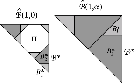
Refer to caption
Figure 19: Return orbits for superscript{\mathcal{B}}\rightarrow{\mathcal{B}}^{*}, s=0𝑠0s=0 (left) and s=α𝑠𝛼s=\alpha (right).

Turning now to the other endpoint, we assume =^(1,α)^1𝛼{\mathcal{B}}=\widehat{{\mathcal{B}}}(1,\alpha). The data for this dressed domain and its atoms B3subscript𝐵3B_{3}, B4subscript𝐵4B_{4}, and B5subscript𝐵5B_{5} are displayed in table 1 with l=1,h=αformulae-sequence𝑙1𝛼l=1,\;h=\alpha. By direct iteration of ρsubscript𝜌superscriptabsent\rho_{\stackrel{{\scriptstyle}}{{{{\mathcal{B}}}}}} on the tiles

B1subscriptsuperscript𝐵1\displaystyle B^{*}_{1} =\displaystyle= 𝚃(0,2β)𝚁5Q1(αβ),subscript𝚃02𝛽subscript𝚁5subscript𝑄1𝛼𝛽\displaystyle\mathtt{T}_{(0,-2\beta)}\mathtt{R}_{5}Q_{1}(\alpha\beta),
B2subscriptsuperscript𝐵2\displaystyle B^{*}_{2} =\displaystyle= 𝚃(0,2α)𝚁3Q7(2),subscript𝚃02𝛼subscript𝚁3subscript𝑄72\displaystyle\mathtt{T}_{(0,-2\alpha)}\mathtt{R}_{3}Q_{7}(2),

one verifies that the two orbits tile the spanning domain of {\mathcal{B}} (see figure 19), and produce a return map which promotes B3subscript𝐵3B_{3} to a negative-parity dressed domain superscript{\mathcal{B}}^{*} congruent to ^(1,0)^10\widehat{{\mathcal{B}}}(1,0). The incidence matrix is given in Appendix C.

\Box

Proof of theorem 1, statement ii)ii), for i=±1𝑖plus-or-minus1i=\pm 1. The parameter values s=Δ1=Δ0=β𝑠subscriptΔ1subscriptΔ0𝛽s=\Delta_{-1}=\Delta_{0}=\beta and s=Δ1=1𝑠subscriptΔ11s=\Delta_{1}=1 are distinguished from the other cases of scenario I by the presence of two higher-level base triangles with disjoint return orbits, both of which are needed to complete the tiling of the parent base triangle. The case s=β𝑠𝛽s=\beta is proved by direct iteration according to Tiling Plan 2, which is reported in Appendix B and illustrated in figure 20; the treatment of s=1𝑠1s=1 is included in the Electronic Supplement. \Box

An important consequence of this is the splitting of the exceptional set into disjoint ergodic components. Such a behaviour, already observed in quadratic two-dimensional piecewise isometries [11] here takes a very simple form. Moreover, infinitely many examples of it appear in our family, corresponding to the set of all accumulation points, at βksuperscript𝛽𝑘\beta^{k} and αβk,k=1,2,formulae-sequence𝛼superscript𝛽𝑘𝑘12\alpha-\beta^{k},\;k=1,2,\ldots. (The cases with k>1𝑘1k>1 belong to scenario II, to be treated later.)
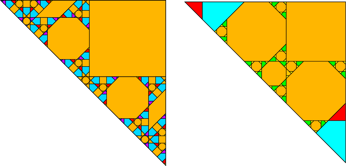
Refer to caption
Figure 20: Illustration of the complete tiling of B(1,s)B1𝑠\mathrm{B}(1,s) by the return orbits of the higher-level base triangle(s) and a finite number of periodic domains. The tiling on the left is for s=107/200I0,1𝑠107200subscript𝐼01s=107/200\in I_{0,-1}, while that on the right is for the accumulation point s=β𝑠𝛽s=\beta.

Proof of proposition 2. For all finite (i,j)𝑖𝑗(i,j) of scenario I, we prove the renormalization superscript\mathcal{B}\to\mathcal{B}^{*} by direct iteration of the domain map ρsubscript𝜌superscriptabsent\rho_{\stackrel{{\scriptstyle}}{{{\mathcal{B}}}}}. Let us illustrate the salient features of the calculations in the case (i,j)=(0,1)𝑖𝑗01(i,j)=(0,-1), corresponding to sI0,1=(β+β3,αβ]𝑠subscript𝐼01𝛽superscript𝛽3𝛼𝛽s\in I_{0,-1}=(\beta+\beta^{3},\alpha\beta]. The corresponding Tiling Plan 1, shown in Appendix B, has been validated using the procedure specified in section 2.5. Extension of these results to the endpoint αβ𝛼𝛽\alpha\beta is straightforward, requiring us to ignore those tiles of superscript{\mathcal{B}}^{*} and periodic domains of Tiling Plan 1 which degenerate to lower-dimensional objects, and allow for the possibility of redundant edge conditions in the specification of tile shapes. In the present example, only 6 of the original 14 tiles survive at the endpoint, with superscript{\mathcal{B}}^{*} degenerating to a two-atom right triangle, as it should in accordance with the vanishing of r(αβ)𝑟𝛼𝛽r(\alpha\beta). Even though superscript{\mathcal{B}}^{*} for s=αβ𝑠𝛼𝛽s=\alpha\beta has only two atoms, their return paths are the same as in the open interval, and their incidence matrix is formed by the first two columns of the 5×5555\times 5 matrix M(0,1)M01{\rm M}(0,-1) displayed in Appendix C.

The tiling plans for the remaining (i,j)𝑖𝑗(i,j)-values of scenario I𝐼I are analogous. Equivalent data tables will be found in the Electronic Supplement, while the corresponding incidence matrices are listed in Appendix C.

10.3 Proof of 𝒫𝒫\mathcal{B}\to\mathcal{P} (scenarios II and IV)

Scenarios II and IV deal with the peripheral parts of the s𝑠s-interval, namely sαβ2𝑠𝛼superscript𝛽2s\leqslant\alpha\beta^{2} and sααβ2=2αβ𝑠𝛼𝛼superscript𝛽22𝛼𝛽s\geqslant\alpha-\alpha\beta^{2}=2\alpha\beta. In these regions we find asymptotic phenomena, which develop at the accumulation points of the singularities of the renormalization function r𝑟r. The analysis is divided into two cases (see figure 10). In Scenario II, the index |i|𝑖|i| diverges while j𝑗j remains within small bounds, so that s𝑠s approaches one of the accumulation points s=0,α𝑠0𝛼s=0,\alpha of f𝑓f, without approaching the first-order accumulation points s=βk𝑠superscript𝛽𝑘s=\beta^{k} or αβk𝛼superscript𝛽𝑘\alpha-\beta^{k}. Scenario IV deals with larger values of |j|𝑗|j|, and includes all doubly asymptotic cases: |i|,|j|𝑖𝑗|i|,|j|\to\infty. We shall establish the following result (the set IV is defined in (28), p. 28):

Proposition 3

Let (i,j)IIIV𝑖𝑗IIIV(i,j)\subset{\rm II}\cup{\rm IV}, let sIi,j𝑠subscript𝐼𝑖𝑗s\in I_{i,j}, and let ^(1,s)similar-to^1𝑠{\mathcal{B}}\sim\widehat{{\mathcal{B}}}(1,s). Then

𝒫𝒫^(α,s),withπ(𝒫)=1.formulae-sequence𝒫similar-to^𝒫𝛼𝑠with𝜋𝒫1{\mathcal{B}}\rightarrow{\mathcal{P}}\sim\widehat{{\mathcal{P}}}(\alpha,s),\;\mbox{with}\;\;\pi({\mathcal{P}})=1. (58)

Moreover,

𝒫𝒫{𝒫^(β|i|1α,s),withπ(𝒫)=(1)|i|1,ifij>0,𝒫^(β|i|2α,s),withπ(𝒫)=(1)|i|,ifij0.𝒫superscript𝒫similar-tocasesformulae-sequence^𝒫superscript𝛽𝑖1𝛼𝑠with𝜋superscript𝒫superscript1𝑖1if𝑖𝑗0formulae-sequence^𝒫superscript𝛽𝑖2𝛼𝑠with𝜋superscript𝒫superscript1𝑖if𝑖𝑗0{\mathcal{P}}\rightarrow{\mathcal{P}}^{*}\sim\left\{\begin{array}[]{l}\widehat{{\mathcal{P}}}(\beta^{|i|-1}\alpha,s),\quad\mbox{with}\quad\pi({\mathcal{P}}^{*})=(-1)^{|i|-1},\quad\mbox{if}\;\;i\cdot j>0,\\ \widehat{{\mathcal{P}}}(\beta^{|i|-2}\alpha,s),\quad\mbox{with}\quad\pi({\mathcal{P}}^{*})=(-1)^{|i|},\quad\mbox{if}\quad i\cdot j\leq 0.\end{array}\right. (59)

The incidence matrix for the combined renormalization step 𝒫superscript𝒫{\mathcal{B}}\rightarrow{\mathcal{P}}^{*} is given by (62).


Proof. The proof of (58)58(\ref{eq:BP}), including the calculation of the incidence matrix, is performed separately for the s𝑠s intervals (0,αβ3)0𝛼superscript𝛽3(0,\alpha\beta^{3}), [αβ3,αβ2]𝛼superscript𝛽3𝛼superscript𝛽2[\alpha\beta^{3},\alpha\beta^{2}], and [2αβ,α)2𝛼𝛽𝛼[2\alpha\beta,\alpha).

Proof of (58) for s(0,αβ3]𝑠0𝛼superscript𝛽3s\in(0,\alpha\beta^{3}]. We prove (58) in two stages. The first, non-branching, stage involves the disjoint return orbits of a fixed number of initial tiles. As s𝑠s ranges over the interval of interest, the orbits evolve continuously without bifurcations. The second stage of the proof deals with all of the s𝑠s-dependent branching, which is entirely accounted for by the transfer-map dynamics of an arrowhead dressed domain 𝒜=(A,𝐀,ρ𝒜)𝒜A𝐀subscript𝜌superscript𝒜absent{\mathcal{A}}=(\mathrm{A},\mathbf{A},\rho_{\stackrel{{\scriptstyle}}{{\mathcal{A}}}}) congruent to 𝒜^(αβ2,s)^𝒜𝛼superscript𝛽2𝑠\widehat{{\mathcal{A}}}(\alpha\beta^{2},s).

Refer to caption
Figure 21: Joint return-map partition of pencil P𝑃P and arrowhead A𝐴A. Those atoms of the pencil’s return map which reside in the quadrilateral Pinsubscript𝑃inP_{\rm in} are mapped, via three iterations of ρBsubscript𝜌𝐵\rho_{B}, into the entrance tile of the arrowhead A𝐴A. The transfer map ψ(r,h)𝜓𝑟\psi(r,h) for A𝐴A then maps them onto the exit tile (dark grey). From there, they are mapped back into P𝑃P by a single application of ρBsubscript𝜌𝐵\rho_{B}.

The non-branching part of the proof establishes the first-return orbits of the disconnected domain PAPA{\rm P}\cup{\rm A}. This set includes the persistent orbits of P0,,P6subscript𝑃0subscript𝑃6P_{0},\ldots,P_{6}, which begin and end in PP{\rm P}, never entering the arrowhead. In addition, we have Pinsubscript𝑃inP_{\rm in} (the complement of i=06Pisuperscriptsubscript𝑖06subscript𝑃𝑖\cup_{i=0}^{6}P_{i} in PP{\rm P}, ignoring boundaries), whose return orbit ends on the entrance tile of 𝒜𝒜{\mathcal{A}}. The set of atoms is rounded out by the three tiles of 𝐀𝐀{\bf A}. Of these, A1subscript𝐴1A_{1} and A3subscript𝐴3A_{3} have orbits which return to AA{\rm A} without entering PP{\rm P}, while that of A2subscript𝐴2A_{2} ends up on 𝚄0Pinsubscript𝚄0subscript𝑃in{\tt U}_{0}P_{\rm in}. All of these statements are proved by direct iteration, with the Tiling Plan 3. We will use the notation ρ𝒫,𝒜subscript𝜌superscript𝒫𝒜absent\rho_{\stackrel{{\scriptstyle}}{{{\mathcal{P}},{\mathcal{A}}}}} for the joint return map.

It remains to establish the s𝑠s-dependent partition of Pinsubscript𝑃inP_{\rm in} and piecewise isometric mapping of Pinsubscript𝑃inP_{\rm in} under ρ𝒫subscript𝜌superscript𝒫absent\rho_{\stackrel{{\scriptstyle}}{{{\mathcal{P}}}}}. The restriction of the latter to Pinsubscript𝑃inP_{\rm in} is given by

ρ𝒫|Pin=ρ𝒫,𝒜ψ𝒜ρ𝒫,𝒜evaluated-atsubscript𝜌superscript𝒫absentsubscript𝑃insubscript𝜌superscript𝒫𝒜absentsubscript𝜓superscript𝒜absentsubscript𝜌superscript𝒫𝒜absent\left.\rho_{\stackrel{{\scriptstyle}}{{{\mathcal{P}}}}}\right|_{P_{\rm in}}=\rho_{\stackrel{{\scriptstyle}}{{{\mathcal{P}},{\mathcal{A}}}}}\circ\psi_{\stackrel{{\scriptstyle}}{{{\mathcal{A}}}}}\circ\rho_{\stackrel{{\scriptstyle}}{{{\mathcal{P}},{\mathcal{A}}}}} (60)

where ψ𝒜subscript𝜓𝒜\psi_{\mathcal{A}} is the arrowhead transfer map. According to the Arrowhead Lemma (section 9), the map ψ𝒜subscript𝜓superscript𝒜absent\psi_{\stackrel{{\scriptstyle}}{{{\mathcal{A}}}}} partitions the entrance tile of 𝒜𝒜^(αβ2,s)similar-to𝒜^𝒜𝛼superscript𝛽2𝑠{\mathcal{A}}\sim\widehat{{\mathcal{A}}}(\alpha\beta^{2},s) into a strip congruent to 𝐒^(αβ2,s)^𝐒𝛼superscript𝛽2𝑠\widehat{\mathbf{S}}(\alpha\beta^{2},s). Since ρ𝒫,𝒜subscript𝜌superscript𝒫𝒜absent\rho_{\stackrel{{\scriptstyle}}{{{\mathcal{P}},{\mathcal{A}}}}} acts on each atom as an orientation-preserving isometry, the atoms contained in Pinsubscript𝑃inP_{\rm in} inherit the strip structure. This is precisely what is needed to fill out the specification of the tiling of 𝒫𝒫^(α,s)similar-to𝒫^𝒫𝛼𝑠{\mathcal{P}}\sim\widehat{{\mathcal{P}}}(\alpha,s). Finally, it is easy to verify that the composition of maps in (60) provides the correct mapping ρ𝒫subscript𝜌superscript𝒫absent\rho_{\stackrel{{\scriptstyle}}{{{\mathcal{P}}}}} of the atoms in Pinsubscript𝑃inP_{\rm in}.

The temporal scaling information of the induction 𝒫𝒫{\mathcal{B}}\rightarrow{\mathcal{P}} is neatly summarized in an incidence matrix Mϵ(𝒫)subscriptMitalic-ϵ𝒫{\rm M}_{\epsilon}({\mathcal{B}}\to{\mathcal{P}}). For each of the persistent atoms Pk,k=0,,6formulae-sequencesubscript𝑃𝑘𝑘06P_{k},\;k=0,\ldots,6, one lists in the relevant column of Mϵ(𝒫)subscriptMitalic-ϵ𝒫{\rm M}_{\epsilon}({\mathcal{B}}\to{\mathcal{P}}) the number of times the return orbit of Pksubscript𝑃𝑘P_{k} visits each of the five atoms of 𝐁𝐁{\bf B}. This information is tallied in the course of the CAP validation. For the remaining atoms, the same data set provides the tile counts for the partial orbits to and from the arrowhead, as well as the the tile counts for the return orbits of the arrowhead atoms. Combining this with the incidence matrix (LABEL:eq:NEk) for the arrowhead transfer map (Arrowhead Lemma, part iii)iii)), we obtain the rest of Mϵ(𝒫)subscriptMitalic-ϵ𝒫{\rm M}_{\epsilon}({\mathcal{B}}\to{\mathcal{P}}). The result is

Mϵ(𝒫)=P0P1P2P3P4P5P6P2k1P2k4kLB1011ϵ1ϵ000akckB20000163bkdkB3111111111B4001000000B5000100000subscriptMitalic-ϵ𝒫missing-subexpressionsubscript𝑃0subscript𝑃1subscript𝑃2subscript𝑃3subscript𝑃4subscript𝑃5subscript𝑃6superscriptsubscript𝑃2𝑘1subscript𝑃2𝑘4𝑘𝐿missing-subexpressionmissing-subexpressionmissing-subexpressionmissing-subexpressionmissing-subexpressionmissing-subexpressionmissing-subexpressionmissing-subexpressionmissing-subexpressionmissing-subexpressionsubscript𝐵1011italic-ϵ1italic-ϵ000subscript𝑎𝑘subscript𝑐𝑘subscript𝐵20000163subscript𝑏𝑘subscript𝑑𝑘subscript𝐵3111111111subscript𝐵4001000000subscript𝐵5000100000{\rm M}_{\epsilon}({\mathcal{B}}\to{\mathcal{P}})=\begin{array}[]{c|ccccccccc}&P_{0}&P_{1}&P_{2}&P_{3}&P_{4}&P_{5}&P_{6}&\lx@intercol\hfil\overbrace{P_{2k-1}\;P_{2k}}^{4\leqslant k\leqslant L}\hfil\lx@intercol\\ \hline\cr B_{1}&0&1&1-\epsilon&1-\epsilon&0&0&0&a_{k}&c_{k}\\ B_{2}&0&0&0&0&1&6&3&b_{k}&d_{k}\\ B_{3}&1&1&1&1&1&1&1&1&1\\ B_{4}&0&0&1&0&0&0&0&0&0\\ B_{5}&0&0&0&1&0&0&0&0&0\end{array} (61)

where ϵ=i/|i|italic-ϵ𝑖𝑖\epsilon=i/|i|, L=|i|+3𝐿𝑖3L=|i|+3, and

ak=12+(1)k+123k2,ck=12+14(1)k+143k2,bk=12(1)k+3k2,dk=112(1)k+123k2.subscript𝑎𝑘12superscript1𝑘12superscript3𝑘2subscript𝑐𝑘1214superscript1𝑘14superscript3𝑘2subscript𝑏𝑘12superscript1𝑘superscript3𝑘2subscript𝑑𝑘112superscript1𝑘12superscript3𝑘2\begin{array}[]{ll}a_{k}=-\frac{1}{2}+(-1)^{k}+\frac{1}{2}\cdot 3^{k-2},&c_{k}=-\frac{1}{2}+\frac{1}{4}(-1)^{k}+\frac{1}{4}\cdot 3^{k-2},\\ b_{k}=1-2(-1)^{k}+3^{k-2},&d_{k}=1-\frac{1}{2}(-1)^{k}+\frac{1}{2}\cdot 3^{k-2}.\end{array}

The return times for the pencil’s atoms, expressed in terms of iterations of ρBsubscript𝜌𝐵\rho_{B}, are obtained by summing the respective columns of the incidence matrix. We have established the completeness of the tiling by return orbits of the pencil and arrowhead by calculating the total area of each return orbit (area of the source polygon multiplied by the return time), summing over all orbits, including the periodic one, and comparing with the area of BB{\rm B}. Note that it is unnecessary to consider anew the periodic orbits which pass through the arrowhead, since these are subsumed in the recursive tiling property of the arrowhead proved in section 9.


Proof of (58) and (61) for s[αβ3,αβ2]𝑠𝛼superscript𝛽3𝛼superscript𝛽2s\in[\alpha\beta^{3},\alpha\beta^{2}]. On this interval, the pencil 𝒫𝒫{\mathcal{P}} is minimal, with precisely 9 atoms. Here, the mediation of an arrowhead is not needed, and we prove the renormalization step and incidence matrix using the method of direct iteration. The statement and validation of the tiling scheme (from which the incidence matrix (61) can be verified) may be found in the Electronic Supplement [6].


Proof of (58) for s[2αβ,α)𝑠2𝛼𝛽𝛼s\in[2\alpha\beta,\alpha). Consider now the relation between a value of s𝑠s in (0,αβ2]0𝛼superscript𝛽2(0,\alpha\beta^{2}] and its mirror value s~=αs~𝑠𝛼𝑠\tilde{s}=\alpha-s. In the latter case, the return-map partition of B3(s~)subscript𝐵3~𝑠B_{3}(\tilde{s}) (the third atom of ^(1,s)^1𝑠\widehat{{\mathcal{B}}}(1,s) in the canonical ordering of table 1) is very far from being pencil-like. On the other hand, one of the five atoms of B3(s~)subscript𝐵3~𝑠B_{3}(\tilde{s}) is in fact a pencil P~~𝑃\tilde{P} with the same parameters and same return-map (up to placement) as P=B3(s)𝑃subscript𝐵3𝑠P=B_{3}(s).

We first compare explicitly the return orbits of tiles P2subscript𝑃2P_{2} and P3subscript𝑃3P_{3} to those of P~2subscript~𝑃2\tilde{P}_{2} and P~3subscript~𝑃3\tilde{P}_{3}. They are different, but lead to the same image tiles, up to placement, after returning to the pencil.

Now let us remove tiles #2 and #3 from the game and consider how to construct the return orbits of the remaining tiles of each pencil. These orbits will visit only the tiles B1(s)subscript𝐵1𝑠B_{1}(s) and B2(s)subscript𝐵2𝑠B_{2}(s) (respectively, B31(s~)subscript𝐵31~𝑠B_{31}(\tilde{s}) and B32(s~)subscript𝐵32~𝑠B_{32}(\tilde{s}), the sub-tiles 1 and 2 of B3(s~)subscript𝐵3~𝑠B_{3}(\tilde{s})) before returning to the pencil, since the remaining two tiles lie on the orbits of tiles #2 and #3. Now B1(s)subscript𝐵1𝑠B_{1}(s) and B31(s~)subscript𝐵31~𝑠B_{31}(\tilde{s}) are congruent and the action of the respective mappings on them are the same, up to placement. If the overlaps of B2(s)subscript𝐵2𝑠B_{2}(s) with the orbits of #2 and #3 are deleted, then the truncated polygon is found to be congruent to B32(s~)subscript𝐵32~𝑠B_{32}(\tilde{s}), and once again the mappings are the same, up to placement. Thus the return orbits of all the remaining tiles of the two pencils are identical, up to placement. The above arguments are illustrated in figure 22
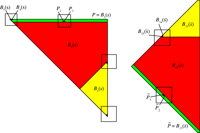
Refer to caption
Figure 22: Return orbits of pencil tiles #2 and #3, shown in boxes against the background of the return-map partitions of B1(s)subscript𝐵1𝑠B_{1}(s) (on left) and B13(s~)subscript𝐵13~𝑠B_{13}(\tilde{s}), for a value of s~~𝑠\tilde{s} near 1.3. Note that once the two orbits are deleted, the effective domain maps needed to calculate the return orbits of the remaining pencil tiles are conjugate via a rotation and translation.

For the mirror intervals with s2αβ𝑠2𝛼𝛽s\geqslant 2\alpha\beta, the 𝒫𝒫{\mathcal{B}}\rightarrow{\mathcal{P}} incidence matrix is again given by (61), with ϵ=1italic-ϵ1\epsilon=1.

Proof of (59). The proof is a direct application of the Pencil Shortening Lemma (section 8.2). Multiplying the incidence matrices for 𝒫𝒫{\mathcal{B}}\rightarrow{\mathcal{P}} and 𝒫𝒫𝒫superscript𝒫{\mathcal{P}}\rightarrow{\mathcal{P}}^{*}, we obtain, for s(0,αβ2][2αβ,α)𝑠0𝛼superscript𝛽22𝛼𝛽𝛼s\in(0,\alpha\beta^{2}]\cup[2\alpha\beta,\alpha),

Mϵ(𝒫)=(01212ϵ(i)2|i|21212121212014|i|6411111119411111001000000000000000)+subscriptMitalic-ϵsuperscript𝒫limit-from01212italic-ϵ𝑖2𝑖21212121212014𝑖6411111119411111001000000000000000{\rm M}_{\epsilon}({\mathcal{B}}\to{\mathcal{P}}^{*})=\left(\begin{array}[]{ccccccccc}0&-\frac{1}{2}&\frac{1}{2}-\epsilon(i)-2|i|&-2&-\frac{1}{2}&-\frac{1}{2}&-\frac{1}{2}&-\frac{1}{2}&-\frac{1}{2}\\ 0&1&4|i|-6&4&1&1&1&1&1\\ 1&1&9&4&1&1&1&1&1\\ 0&0&1&0&0&0&0&0&0\\ 0&0&0&0&0&0&0&0&0\end{array}\right)+
(013432141141140232312212212000000000000000000000000000)(1)i+limit-from013432141141140232312212212000000000000000000000000000superscript1𝑖\left(\begin{array}[]{ccccccccc}0&-1&-\frac{3}{4}&-\frac{3}{2}&-\frac{1}{4}&1&\frac{1}{4}&-1&-\frac{1}{4}\\ 0&2&\frac{3}{2}&3&\frac{1}{2}&-2&-\frac{1}{2}&2&\frac{1}{2}\\ 0&0&0&0&0&0&0&0&0\\ 0&0&0&0&0&0&0&0&0\\ 0&0&0&0&0&0&0&0&0\end{array}\right)\,(-1)^{i}+ (62)
(01671271811212143234013767916112332000000000000000000000000000) 3|i|01671271811212143234013767916112332000000000000000000000000000superscript3𝑖\left(\begin{array}[]{ccccccccc}0&\frac{1}{6}&\frac{7}{12}&\frac{7}{18}&\frac{1}{12}&\frac{1}{2}&\frac{1}{4}&\frac{3}{2}&\frac{3}{4}\\ 0&\frac{1}{3}&\frac{7}{6}&\frac{7}{9}&\frac{1}{6}&1&\frac{1}{2}&3&\frac{3}{2}\\ 0&0&0&0&0&0&0&0&0\\ 0&0&0&0&0&0&0&0&0\\ 0&0&0&0&0&0&0&0&0\end{array}\right)\,3^{|i|}

10.4 Proof of 𝒫superscript𝒫superscript{\mathcal{P}}^{*}\rightarrow{\mathcal{B}}^{*} (scenario II)

Scenario II includes both a countable set of accumulation points, namely Δi,|i|2subscriptΔ𝑖𝑖2\Delta_{i},\;|i|\geqslant 2, as well as a subset of the continuity intervals, Ii,jsubscript𝐼𝑖𝑗I_{i,j}, i,j𝑖𝑗i,j finite. In the former case, the renormalization is described by statement (ii) of theorem 1, while the latter case is handled by the following proposition:

Proposition 4

Let (i,j)II2𝑖𝑗IIsuperscript2(i,j)\in{\rm II}\cap\mathbb{Z}^{2}, let sIi,j𝑠subscript𝐼𝑖𝑗s\in I_{i,j}, and let 𝒫superscript𝒫{\mathcal{P}}^{*} be as in (59). Then 𝒫superscript𝒫superscript{\mathcal{P}}^{*}\rightarrow{\mathcal{B}}^{*} where

^(l,r(s)l),withl=β|i|+|j|+2,π()=(1)|i|+|j|.formulae-sequencesimilar-tosuperscript^superscript𝑙𝑟𝑠superscript𝑙withformulae-sequencesuperscript𝑙superscript𝛽𝑖𝑗2𝜋superscriptsuperscript1𝑖𝑗{\mathcal{B}}^{*}\sim\widehat{{\mathcal{B}}}(l^{*},r(s)l^{*}),\quad\mbox{with}\quad l^{*}=\beta^{|i|+|j|+2},\;\pi({\mathcal{B}}^{*})=(-1)^{|i|+|j|}. (63)

The incidence matrices for this renormalization step are listed in Appendix D.

Proof. Thanks to the scale invariance of the dynamics, it is sufficient to restrict ourselves to the values of s𝑠s (both the accumulation points and the continuity intervals) where the pencil is minimal. These are handled on a case-by-case basis by direct iteration, exactly as was done for scenario I. Again, we relegate the tiling plans to the Electronic Supplement, with the exception of those for the accumulation points s=βk,k=2,3,formulae-sequence𝑠superscript𝛽𝑘𝑘23s=\beta^{k},\;k=2,3,\ldots, where tiling of the pencil requires two return orbits of higher-level base triangles (see Tiling Plan 4 and figure 23). For the sake of the completeness of the scaling data, we list all the relevant incidence matrices in Appendices D and F.

Refer to caption
Figure 23: Tiling of the minimal pencil by two disjoint return orbits of s=0𝑠0s=0 base triangles, plus several periodic orbits.

10.5 Proof of 𝒯μsubscript𝒯𝜇\mathcal{B}\to\mathcal{T}_{\mu} (scenarios III and IV)

Proposition 5

Let (i,j)IIIIV𝑖𝑗IIIIV(i,j)\in{\rm III}\cup{\rm IV} (see equation (28)), let sIi,j𝑠subscript𝐼𝑖𝑗s\in I_{i,j}, and let ^(1,s)similar-to^1𝑠{\mathcal{B}}\sim\widehat{{\mathcal{B}}}(1,s). Then 𝒯μ(i,j)subscript𝒯𝜇𝑖𝑗{\mathcal{B}}\rightarrow{\mathcal{T}}_{\mu(i,j)}, where μ(i,j)𝜇𝑖𝑗\mu(i,j) is as in table 2 p. 2, and

𝒯subscript𝒯\displaystyle{\mathcal{T}}_{-} similar-to\displaystyle\sim 𝒯^(β|i|+1,sβ|i|+1),withπ(𝒯)=(1)|i|,subscript^𝒯superscript𝛽𝑖1𝑠superscript𝛽𝑖1with𝜋subscript𝒯superscript1𝑖\displaystyle\widehat{{\mathcal{T}}}_{-}(\beta^{|i|+1},s-\beta^{|i|+1}),\;\mbox{with}\;\pi({\mathcal{T}}_{-})=(-1)^{|i|}, (64)
𝒯+subscript𝒯\displaystyle{\mathcal{T}}_{+} similar-to\displaystyle\sim 𝒯^+(β|i|+2,β|i|s),withπ(𝒯+)=(1)|i|+1.subscript^𝒯superscript𝛽𝑖2superscript𝛽𝑖𝑠with𝜋subscript𝒯superscript1𝑖1\displaystyle\widehat{{\mathcal{T}}}_{+}(\beta^{|i|+2},\beta^{|i|}-s),\;\;\;\mbox{with}\;\;\pi({\mathcal{T}}_{+})=(-1)^{|i|+1}.

The relevant incidence matrices are given in formulae (66)–(71).

Proof. We start with scenario IIIμν, with s[ββ6,β)(β,β+β4]𝑠𝛽superscript𝛽6𝛽𝛽𝛽superscript𝛽4s\in[\beta-\beta^{6},\beta)\cup(\beta,\beta+\beta^{4}], corresponding to i=0𝑖0i=0 for 𝒯subscript𝒯{\mathcal{T}}_{-} and i=1𝑖1i=-1 for 𝒯+subscript𝒯{\mathcal{T}}_{+} in (64). Our first task is to prove that the return map for B1subscript𝐵1B_{1},the first atom of ^(1,s)^1𝑠\widehat{{\mathcal{B}}}(1,s), promotes the triangle to a fringed triangle of type 𝒯^(β,sβ)subscript^𝒯𝛽𝑠𝛽\widehat{{\mathcal{T}}}_{-}(\beta,s-\beta) (resp. 𝒯^+(β3,βs))\widehat{{\mathcal{T}}}_{+}(\beta^{3},\beta-s)). To help establish this, we introduce an auxiliary arrowhead (analogous to that introduced in section 10.3) and prove by direct iteration that the induced domain map is the correct one. The non-branching part of the return-map proof, valid for all s𝑠s in the chosen interval and illustrated in figure 24, is accomplished with computer assistance, according to the Tiling Plans 5 and 6. There T±=B1superscriptTplus-or-minussubscript𝐵1{\rm T}^{\pm}=B_{1}, and T1,,T4subscriptsuperscript𝑇1subscriptsuperscript𝑇4T^{-}_{1},\ldots,T^{-}_{4} (resp. T1,,T7subscriptsuperscript𝑇1subscriptsuperscript𝑇7T^{-}_{1},\ldots,T^{-}_{7}) are atoms whose return orbits are non-branching. The domain Tin±subscriptsuperscript𝑇plus-or-minusinT^{\pm}_{\rm in} is a ‘blank’ polygon which is delivered by the computer program to the entrance tile of the arrowhead. Arrowhead dynamics endows the polygon with the (s𝑠s-dependent) structure of a strip, and maps it to the exit domain A2subscript𝐴2A_{2}, from which it is delivered, isometrically to its final destination in TT{\rm T} by the computer program. The completeness of the tiling is checked by summing the areas of all tiles contained in the computer-generated orbits of the source domains.
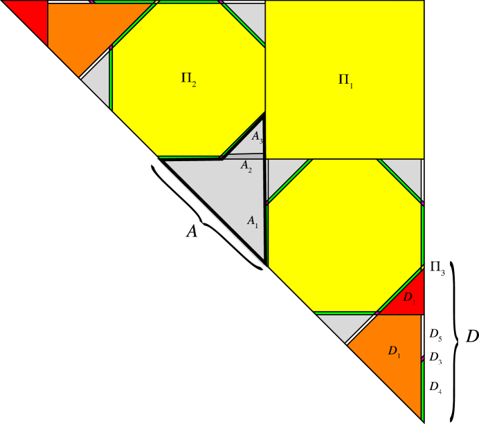
Refer to caption
Figure 24: Tiling of the base for scenario III, according to the Tiling Plan 7.

An analogous treatment for s𝑠s in the mirror interval [1β4,1+β6]1superscript𝛽41superscript𝛽6[1-\beta^{4},1+\beta^{6}] can be given, with the tiling domain T±=B5superscriptTplus-or-minussubscript𝐵5{\rm T}^{\pm}=B_{5}, the fifth atom of ^(1,s)^1𝑠\widehat{{\mathcal{B}}}(1,s). The tiling schemes, which are very similar to Tiling Plans 5 and 6, have been relegated to the Electronic Supplement. Once again, however, we list all the incidence matrices, using a superscript to indicate the sign of index i𝑖i. Moreover, it is useful, from here on, to introduce a parameter

K=|j|(μ(i,j)+1)/2.𝐾𝑗𝜇𝑖𝑗12K=|j|-(\mu(i,j)+1)/2. (65)

In the current context, this will be used to keep track of the numbers of atoms in the various parametric dressed domains.

For negative i𝑖i, we have the scenario III incidence matrices

M(𝒯)=T1T2T2k1T2k2kK+2B11111B200akckB300bkdkB40122B51000subscriptMabsent𝒯missing-subexpressionsubscriptsuperscript𝑇1subscriptsuperscript𝑇2superscriptsubscriptsuperscript𝑇2𝑘1subscriptsuperscript𝑇2𝑘2𝑘𝐾2missing-subexpressionmissing-subexpressionmissing-subexpressionmissing-subexpressionmissing-subexpressionsubscript𝐵11111subscript𝐵200subscript𝑎𝑘subscript𝑐𝑘subscript𝐵300subscript𝑏𝑘subscript𝑑𝑘subscript𝐵40122subscript𝐵51000{\rm M}_{--}({\mathcal{B}}\to{\mathcal{T}})=\begin{array}[]{c|cccc}&T^{-}_{1}&T^{-}_{2}&\lx@intercol\hfil\overbrace{T^{-}_{2k-1}\;T^{-}_{2k}}^{2\leqslant k\leqslant K+2}\hfil\lx@intercol\\ \hline\cr B_{1}&1&1&1&1\\ B_{2}&0&0&a_{k}&c_{k}\\ B_{3}&0&0&b_{k}&d_{k}\\ B_{4}&0&1&2&2\\ B_{5}&1&0&0&0\end{array} (66)

where

ak=1+2(1)k+3k1,ck=1+12(1)k+123k1,bk=12+3(1)k+123k1,dk=12+34(1)k+143k1.subscript𝑎𝑘12superscript1𝑘superscript3𝑘1subscript𝑐𝑘112superscript1𝑘12superscript3𝑘1subscript𝑏𝑘123superscript1𝑘12superscript3𝑘1subscript𝑑𝑘1234superscript1𝑘14superscript3𝑘1\begin{array}[]{ll}a_{k}=1+2(-1)^{k}+3^{k-1},&\qquad c_{k}=1+\frac{1}{2}(-1)^{k}+\frac{1}{2}\cdot 3^{k-1},\\ b_{k}=\frac{1}{2}+3(-1)^{k}+\frac{1}{2}\cdot 3^{k-1},&\qquad d_{k}=\frac{1}{2}+\frac{3}{4}(-1)^{k}+\frac{1}{4}\cdot 3^{k-1}.\end{array}
M+(𝒯)=T1+T2+T3+T4+T5+T6+T7+T2k+T2k+1+4kK+4B1111111111B2000101825akckB300171034bkdkB4010000000B5100000000subscriptMabsent𝒯missing-subexpressionsubscriptsuperscript𝑇1subscriptsuperscript𝑇2subscriptsuperscript𝑇3subscriptsuperscript𝑇4subscriptsuperscript𝑇5subscriptsuperscript𝑇6subscriptsuperscript𝑇7superscriptsubscriptsuperscript𝑇2𝑘subscriptsuperscript𝑇2𝑘14𝑘𝐾4missing-subexpressionmissing-subexpressionmissing-subexpressionmissing-subexpressionmissing-subexpressionmissing-subexpressionmissing-subexpressionmissing-subexpressionmissing-subexpressionmissing-subexpressionsubscript𝐵1111111111subscript𝐵2000101825subscript𝑎𝑘subscript𝑐𝑘subscript𝐵300171034subscript𝑏𝑘subscript𝑑𝑘subscript𝐵4010000000subscript𝐵5100000000{\rm M}_{-+}({\mathcal{B}}\to{\mathcal{T}})=\begin{array}[]{c|ccccccccc}&T^{+}_{1}&T^{+}_{2}&T^{+}_{3}&T^{+}_{4}&T^{+}_{5}&T^{+}_{6}&T^{+}_{7}&\lx@intercol\hfil\overbrace{T^{+}_{2k}\;T^{+}_{2k+1}}^{4\leqslant k\leqslant K+4}\hfil\lx@intercol\\ \hline\cr B_{1}&1&1&1&1&1&1&1&1&1\\ B_{2}&0&0&0&10&18&2&5&a_{k}&c_{k}\\ B_{3}&0&0&1&7&10&3&4&b_{k}&d_{k}\\ B_{4}&0&1&0&0&0&0&0&0&0\\ B_{5}&1&0&0&0&0&0&0&0&0\end{array} (67)

where

ak=17+2(1)k+3k1,ck=17+12(1)k+123k1,bk=172+3(1)k+123k1,dk=172+34(1)k+143k1.subscript𝑎𝑘172superscript1𝑘superscript3𝑘1subscript𝑐𝑘1712superscript1𝑘12superscript3𝑘1subscript𝑏𝑘1723superscript1𝑘12superscript3𝑘1subscript𝑑𝑘17234superscript1𝑘14superscript3𝑘1\begin{array}[]{ll}a_{k}=17+2(-1)^{k}+3^{k-1},&\qquad c_{k}=17+\frac{1}{2}(-1)^{k}+\frac{1}{2}\cdot 3^{k-1},\\ b_{k}=\frac{17}{2}+3(-1)^{k}+\frac{1}{2}3^{k-1},&\qquad d_{k}=\frac{17}{2}+\frac{3}{4}(-1)^{k}+\frac{1}{4}\cdot 3^{k-1}.\end{array}

For positive i𝑖i, the corresponding matrices are

M+(𝒯)=T1T2T2k1T2k2kK+2B11000B20122B300akckB400bkdkB51111subscriptMabsent𝒯missing-subexpressionsubscriptsuperscript𝑇1subscriptsuperscript𝑇2superscriptsubscriptsuperscript𝑇2𝑘1subscriptsuperscript𝑇2𝑘2𝑘𝐾2missing-subexpressionmissing-subexpressionmissing-subexpressionmissing-subexpressionmissing-subexpressionsubscript𝐵11000subscript𝐵20122subscript𝐵300subscript𝑎𝑘subscript𝑐𝑘subscript𝐵400subscript𝑏𝑘subscript𝑑𝑘subscript𝐵51111{\rm M}_{+-}({\mathcal{B}}\to{\mathcal{T}})=\begin{array}[]{c|cccc}&T^{-}_{1}&T^{-}_{2}&\lx@intercol\hfil\overbrace{T^{-}_{2k-1}\;T^{-}_{2k}}^{2\leqslant k\leqslant K+2}\hfil\lx@intercol\\ \hline\cr B_{1}&1&0&0&0\\ B_{2}&0&1&2&2\\ B_{3}&0&0&a_{k}&c_{k}\\ B_{4}&0&0&b_{k}&d_{k}\\ B_{5}&1&1&1&1\end{array} (68)

where

ak=12+5(1)k+123k,ck=12+54(1)k+143k,bk=1+2(1)k+3k1,dk=1+12(1)k+123k1.subscript𝑎𝑘125superscript1𝑘12superscript3𝑘subscript𝑐𝑘1254superscript1𝑘14superscript3𝑘subscript𝑏𝑘12superscript1𝑘superscript3𝑘1subscript𝑑𝑘112superscript1𝑘12superscript3𝑘1\begin{array}[]{ll}a_{k}=\frac{1}{2}+5(-1)^{k}+\frac{1}{2}3^{k},&\qquad c_{k}=\frac{1}{2}+\frac{5}{4}(-1)^{k}+\frac{1}{4}3^{k},\\ b_{k}=1+2(-1)^{k}+3^{k-1},&\qquad d_{k}=1+\frac{1}{2}(-1)^{k}+\frac{1}{2}\cdot 3^{k-1}.\end{array}
M++(𝒯)=T1+T2+T3+T4+T5+T6+T7+T2k+T2k+1+4kK+4B1100000000B2010000000B30021829610akckB4000101825bkdkB5111111111subscriptMabsent𝒯missing-subexpressionsubscriptsuperscript𝑇1subscriptsuperscript𝑇2subscriptsuperscript𝑇3subscriptsuperscript𝑇4subscriptsuperscript𝑇5subscriptsuperscript𝑇6subscriptsuperscript𝑇7superscriptsubscriptsuperscript𝑇2𝑘subscriptsuperscript𝑇2𝑘14𝑘𝐾4missing-subexpressionmissing-subexpressionmissing-subexpressionmissing-subexpressionmissing-subexpressionmissing-subexpressionmissing-subexpressionmissing-subexpressionmissing-subexpressionmissing-subexpressionsubscript𝐵1100000000subscript𝐵2010000000subscript𝐵30021829610subscript𝑎𝑘subscript𝑐𝑘subscript𝐵4000101825subscript𝑏𝑘subscript𝑑𝑘subscript𝐵5111111111{\rm M}_{++}({\mathcal{B}}\to{\mathcal{T}})=\begin{array}[]{c|ccccccccc}&T^{+}_{1}&T^{+}_{2}&T^{+}_{3}&T^{+}_{4}&T^{+}_{5}&T^{+}_{6}&T^{+}_{7}&\lx@intercol\hfil\overbrace{T^{+}_{2k}\;T^{+}_{2k+1}}^{4\leqslant k\leqslant K+4}\hfil\lx@intercol\\ \hline\cr B_{1}&1&0&0&0&0&0&0&0&0\\ B_{2}&0&1&0&0&0&0&0&0&0\\ B_{3}&0&0&2&18&29&6&10&a_{k}&c_{k}\\ B_{4}&0&0&0&10&18&2&5&b_{k}&d_{k}\\ B_{5}&1&1&1&1&1&1&1&1&1\end{array} (69)

where

ak=532+5(1)k+123k,ck=532+54(1)k+143k,bk=17+2(1)k+3k1,dk=17+12(1)k+123k1.subscript𝑎𝑘5325superscript1𝑘12superscript3𝑘subscript𝑐𝑘53254superscript1𝑘14superscript3𝑘subscript𝑏𝑘172superscript1𝑘superscript3𝑘1subscript𝑑𝑘1712superscript1𝑘12superscript3𝑘1\begin{array}[]{ll}a_{k}=\frac{53}{2}+5(-1)^{k}+\frac{1}{2}3^{k},&\qquad c_{k}=\frac{53}{2}+\frac{5}{4}(-1)^{k}+\frac{1}{4}3^{k},\\ b_{k}=17+2(-1)^{k}+3^{k-1},&\qquad d_{k}=17+\frac{1}{2}(-1)^{k}+\frac{1}{2}\cdot 3^{k-1}.\end{array}

We now turn to scenario IVμν, where the renormalization process has already reached the minimal pencil stage. The next step, in which fringed triangles are induced, is completely analogous to what we have just studied for 𝒯μsubscript𝒯𝜇{\mathcal{B}}\rightarrow{\mathcal{T}}_{\mu}, again leading to (64). The relevant Tiling Plans 7 and 8 are given in Appendix B for the two values of μ𝜇\mu.

The corresponding incidence matrices are:

M(𝒫𝒯)=T1T2T3T4T2k1T2k3kK+2P0000000P1000000P2012222P3000000P4224444P5111111P60063akdkP70000bkekP80000ckfksubscriptMsuperscript𝒫𝒯missing-subexpressionsubscriptsuperscript𝑇1subscriptsuperscript𝑇2subscriptsuperscript𝑇3subscriptsuperscript𝑇4superscriptsubscriptsuperscript𝑇2𝑘1subscriptsuperscript𝑇2𝑘3𝑘𝐾2missing-subexpressionmissing-subexpressionmissing-subexpressionmissing-subexpressionmissing-subexpressionmissing-subexpressionmissing-subexpressionmissing-subexpressionmissing-subexpressionsubscriptsuperscript𝑃0000000missing-subexpressionsubscriptsuperscript𝑃1000000missing-subexpressionsubscriptsuperscript𝑃2012222missing-subexpressionsubscriptsuperscript𝑃3000000missing-subexpressionsubscriptsuperscript𝑃4224444missing-subexpressionsubscriptsuperscript𝑃5111111missing-subexpressionsubscriptsuperscript𝑃60063subscript𝑎𝑘subscript𝑑𝑘missing-subexpressionsubscriptsuperscript𝑃70000subscript𝑏𝑘subscript𝑒𝑘missing-subexpressionsubscriptsuperscript𝑃80000subscript𝑐𝑘subscript𝑓𝑘missing-subexpression{\rm M}_{-}({\mathcal{P}}^{*}\to{\mathcal{T}})=\begin{array}[]{c|ccccccc}&T^{-}_{1}&T^{-}_{2}&T^{-}_{3}&T^{-}_{4}&\lx@intercol\hfil\overbrace{T^{-}_{2k-1}\;T^{-}_{2k}}^{3\leqslant k\leqslant K+2}\hfil\lx@intercol\\ \hline\cr P^{*}_{0}&0&0&0&0&0&0\\ P^{*}_{1}&0&0&0&0&0&0\\ P^{*}_{2}&0&1&2&2&2&2\\ P^{*}_{3}&0&0&0&0&0&0\\ P^{*}_{4}&2&2&4&4&4&4\\ \ P^{*}_{5}&1&1&1&1&1&1\\ P^{*}_{6}&0&0&6&3&a_{k}&d_{k}\\ P^{*}_{7}&0&0&0&0&b_{k}&e_{k}\\ P^{*}_{8}&0&0&0&0&c_{k}&f_{k}\\ \end{array} (70)

where

ak=1+2(1)k+3k2,dk=1+12(1)k+123k2,bk=12(1)k+123k3,ek=1214(1)k+143k3,ck=1+2(1)k+3k3,fk=1+12(1)k+123k3,subscript𝑎𝑘12superscript1𝑘superscript3𝑘2subscript𝑑𝑘112superscript1𝑘12superscript3𝑘2subscript𝑏𝑘12superscript1𝑘12superscript3𝑘3subscript𝑒𝑘1214superscript1𝑘14superscript3𝑘3subscript𝑐𝑘12superscript1𝑘superscript3𝑘3subscript𝑓𝑘112superscript1𝑘12superscript3𝑘3\begin{array}[]{ll}a_{k}=1+2(-1)^{k}+3^{k-2},&\qquad d_{k}=1+\frac{1}{2}(-1)^{k}+\frac{1}{2}\cdot 3^{k-2},\\ b_{k}=-\frac{1}{2}-(-1)^{k}+\frac{1}{2}\cdot 3^{k-3},&\qquad e_{k}=-\frac{1}{2}-\frac{1}{4}(-1)^{k}+\frac{1}{4}\cdot 3^{k-3},\\ c_{k}=1+2(-1)^{k}+3^{k-3},&\qquad f_{k}=1+\frac{1}{2}(-1)^{k}+\frac{1}{2}\cdot 3^{k-3},\end{array}
M+(𝒫𝒯)=T1+T2+T3+T4+T5+T6+T7+T2k+T2k+1+4kK+4P0000000000P1000000000P2010000000P3000000000P4220000000P5111111111P60004622akdkP70000100bkekP80002201ckfksubscriptMsuperscript𝒫𝒯missing-subexpressionsubscriptsuperscript𝑇1subscriptsuperscript𝑇2subscriptsuperscript𝑇3subscriptsuperscript𝑇4subscriptsuperscript𝑇5subscriptsuperscript𝑇6subscriptsuperscript𝑇7superscriptsubscriptsuperscript𝑇2𝑘subscriptsuperscript𝑇2𝑘14𝑘𝐾4missing-subexpressionmissing-subexpressionmissing-subexpressionmissing-subexpressionmissing-subexpressionmissing-subexpressionmissing-subexpressionmissing-subexpressionmissing-subexpressionmissing-subexpressionmissing-subexpressionmissing-subexpressionmissing-subexpressionmissing-subexpressionmissing-subexpressionmissing-subexpressionsubscriptsuperscript𝑃0000000000missing-subexpressionmissing-subexpressionmissing-subexpressionsubscriptsuperscript𝑃1000000000missing-subexpressionmissing-subexpressionmissing-subexpressionsubscriptsuperscript𝑃2010000000missing-subexpressionmissing-subexpressionmissing-subexpressionsubscriptsuperscript𝑃3000000000missing-subexpressionmissing-subexpressionmissing-subexpressionsubscriptsuperscript𝑃4220000000missing-subexpressionmissing-subexpressionmissing-subexpressionsubscriptsuperscript𝑃5111111111missing-subexpressionmissing-subexpressionmissing-subexpressionsubscriptsuperscript𝑃60004622subscript𝑎𝑘subscript𝑑𝑘missing-subexpressionmissing-subexpressionmissing-subexpressionsubscriptsuperscript𝑃70000100subscript𝑏𝑘subscript𝑒𝑘missing-subexpressionmissing-subexpressionmissing-subexpressionsubscriptsuperscript𝑃80002201subscript𝑐𝑘subscript𝑓𝑘missing-subexpressionmissing-subexpressionmissing-subexpression{\rm M}_{+}({\mathcal{P}}^{*}\to{\mathcal{T}})=\begin{array}[]{c|cccccccccccc}&T^{+}_{1}&T^{+}_{2}&T^{+}_{3}&T^{+}_{4}&T^{+}_{5}&T^{+}_{6}&T^{+}_{7}&\lx@intercol\hfil\overbrace{T^{+}_{2k}\;T^{+}_{2k+1}}^{4\leqslant k\leqslant K+4}\hfil\lx@intercol\\ \hline\cr P^{*}_{0}&0&0&0&0&0&0&0&0&0\\ P^{*}_{1}&0&0&0&0&0&0&0&0&0\\ P^{*}_{2}&0&1&0&0&0&0&0&0&0\\ P^{*}_{3}&0&0&0&0&0&0&0&0&0\\ P^{*}_{4}&2&2&0&0&0&0&0&0&0\\ \ P^{*}_{5}&1&1&1&1&1&1&1&1&1\\ P^{*}_{6}&0&0&0&4&6&2&2&a_{k}&d_{k}\\ P^{*}_{7}&0&0&0&0&1&0&0&b_{k}&e_{k}\\ P^{*}_{8}&0&0&0&2&2&0&1&c_{k}&f_{k}\\ \end{array} (71)

where

ak=5+2(1)k+3k2,dk=5+12(1)k+123k2,bk=32(1)k+123k3,ek=3214(1)k+143k3,ck=1+2(1)k+3k3,fk=1+12(1)k+123k3.subscript𝑎𝑘52superscript1𝑘superscript3𝑘2subscript𝑑𝑘512superscript1𝑘12superscript3𝑘2subscript𝑏𝑘32superscript1𝑘12superscript3𝑘3subscript𝑒𝑘3214superscript1𝑘14superscript3𝑘3subscript𝑐𝑘12superscript1𝑘superscript3𝑘3subscript𝑓𝑘112superscript1𝑘12superscript3𝑘3\begin{array}[]{ll}a_{k}=5+2(-1)^{k}+3^{k-2},&\qquad d_{k}=5+\frac{1}{2}(-1)^{k}+\frac{1}{2}\cdot 3^{k-2},\\ b_{k}=\frac{3}{2}-(-1)^{k}+\frac{1}{2}\cdot 3^{k-3},&\qquad e_{k}=\frac{3}{2}-\frac{1}{4}(-1)^{k}+\frac{1}{4}\cdot 3^{k-3},\\ c_{k}=1+2(-1)^{k}+3^{k-3},&\qquad f_{k}=1+\frac{1}{2}(-1)^{k}+\frac{1}{2}\cdot 3^{k-3}.\end{array}

10.6 Proof of 𝒯μ𝒟μ𝒟νsubscript𝒯𝜇subscript𝒟𝜇superscriptsubscript𝒟𝜈{\mathcal{T}}_{\mu}\rightarrow{\mathcal{D}}_{\mu}\rightarrow{\mathcal{D}}_{\nu}^{*} (scenarios III and IV)

The next phase of scenarios IIIμν and IVμν is the transition from fringed triangle to double-strip, followed by shortening of the strip.

Proposition 6

Let (i,j)IIIIV𝑖𝑗IIIIV(i,j)\in{\rm III}\cup{\rm IV}, let sIi,j𝑠subscript𝐼𝑖𝑗s\in I_{i,j}, and let 𝒯μ(i,j)subscript𝒯𝜇𝑖𝑗{\mathcal{T}}_{\mu(i,j)} be as in (64). Then 𝒯μ(i,j)𝒟μ(i,j)subscript𝒯𝜇𝑖𝑗subscript𝒟𝜇𝑖𝑗{\mathcal{T}}_{\mu(i,j)}\rightarrow{\mathcal{D}}_{\mu(i,j)}, where

𝒟subscript𝒟\displaystyle{\mathcal{D}}_{-} similar-to\displaystyle\sim 𝒟^(β|i|+3,sβ|i|+1),withπ(𝒟)=(1)|i|+1,subscript^𝒟superscript𝛽𝑖3𝑠superscript𝛽𝑖1with𝜋subscript𝒟superscript1𝑖1\displaystyle\widehat{{\mathcal{D}}}_{-}(\beta^{|i|+3},s-\beta^{|i|+1}),\;\mbox{with}\;\pi({\mathcal{D}}_{-})=(-1)^{|i|+1}, (72)
𝒟+subscript𝒟\displaystyle{\mathcal{D}}_{+} similar-to\displaystyle\sim 𝒟^+(β|i|+4,β|i|s),withπ(𝒟+)=(1)|i|,subscript^𝒟superscript𝛽𝑖4superscript𝛽𝑖𝑠with𝜋subscript𝒟superscript1𝑖\displaystyle\widehat{{\mathcal{D}}}_{+}(\beta^{|i|+4},\beta^{|i|}-s),\;\;\;\mbox{with}\;\;\pi({\mathcal{D}}_{+})=(-1)^{|i|},

and the corresponding incidence matrices are given in (75) and (74), Moreover,

𝒟μ(i,j)𝒟ν(j){𝒟^ν(j)(β|i|+|j|,sβ|i|+1),ifμ(i,j)=1,𝒟^ν(j)(β|i|+|j|,β|i|s),ifμ(i,j)=+1,subscript𝒟𝜇𝑖𝑗subscriptsuperscript𝒟𝜈𝑗similar-tocasessubscript^𝒟𝜈𝑗superscript𝛽𝑖𝑗𝑠superscript𝛽𝑖1if𝜇𝑖𝑗1subscript^𝒟𝜈𝑗superscript𝛽𝑖𝑗superscript𝛽𝑖𝑠if𝜇𝑖𝑗1{\mathcal{D}}_{\mu(i,j)}\rightarrow{\mathcal{D}}^{*}_{\nu(j)}\sim\left\{\begin{array}[]{ll}\widehat{{\mathcal{D}}}_{\nu(j)}(\beta^{|i|+|j|},s-\beta^{|i|+1}),&\;\mbox{if}\;\mu(i,j)=-1,\\ \widehat{{\mathcal{D}}}_{\nu(j)}(\beta^{|i|+|j|},\beta^{|i|}-s),&\;\mbox{if}\;\mu(i,j)=+1,\end{array}\right. (73)

with π(𝒟ν(j))=(1)|i|+|j|𝜋subscriptsuperscript𝒟𝜈𝑗superscript1𝑖𝑗\pi({\mathcal{D}}^{*}_{\nu(j)})=(-1)^{|i|+|j|}.


Proof of (72). We begin with the case μ(i,j)=1𝜇𝑖𝑗1\mu(i,j)=-1. Our task is to calculate the return-map orbits of the trapezoidal atom T3subscriptsuperscript𝑇3T^{-}_{3} of the fringed triangle (see figure 13), showing that the corresponding partition is that of a double-strip with the stated parameters. Scale invariance allows us to fix the parameter l𝑙l of the fringed triangle at l=β𝑙𝛽l=\beta and let the parameter hh range over (0,β4]0superscript𝛽4(0,\beta^{4}]. This treats simultaneously all integer values of the index i𝑖i.

The non-branching part of the proof consists of the computer-assisted validation of tiling plan 9 in Appendix B, illustrated in figure 25.
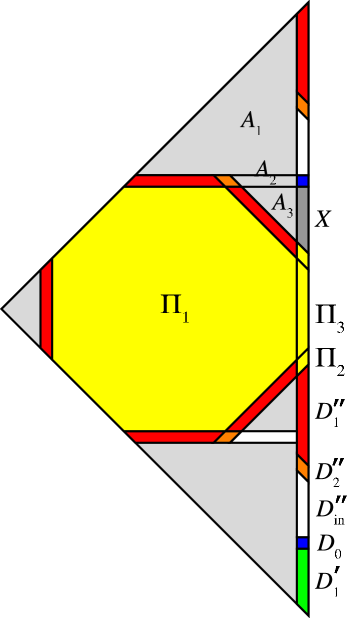
Refer to caption
Figure 25: Tiling of the triangle TsubscriptT{\rm T}_{-}, according to the Tiling Plan 9.

It is worth noting that the induced return map of the double strip corresponds to the variant ν=1𝜈1\nu=-1 (since the double strip has negative parity and a net rotation 𝚁2subscript𝚁2{\tt R}_{2} of atom D0subscript𝐷0D_{0}).

Once again, arrowhead dynamics is responsible for all of the branching, but with an important difference from previous stages of the renormalization. The double strip, labelled 𝒟subscript𝒟{\mathcal{D}}_{-}, has two constituent strips, produced by separate s𝑠s-dependent branching mechanisms. One of these is associated with the arrowhead, while the other is produced by the already established piecewise isometry of proposition 5. It should be emphasized that, as always, computer assistance is enlisted only for the non-branching orbit pieces which are present for all s𝑠s in the chosen interval. This includes the isometric mapping of Dsuperscript𝐷D^{\prime} onto X𝑋X, but not the mapping of X𝑋X back into DD{\rm D} which completes the return orbit.

The case μ(i,j)=+1𝜇𝑖𝑗1\mu(i,j)=+1 is handled in an analogous manner, with the non-branching part of the proof consisting of computer-assisted validation of tiling plan 10. There we identify two special tiles congruent to Dsuperscript𝐷D^{\prime}, namely X𝑋X and Y𝑌Y. The isometric mappings from Dsuperscript𝐷D^{\prime} to X𝑋X and from Y𝑌Y to DDsuperscript𝐷DD^{\prime}\oslash{\rm D} are included in the tiling plan, while the mapping from X𝑋X to Y𝑌Y is a direct application of the domain map of the fringed triangle.

As a by-product of the return-map calculations leading to (72), we obtain the following incidence matrices:

M(𝒯𝒟)=D0D2k1′′D2k′′1jKDl1l2K2T11akck0T20bkdk0T31111T4T60000Tj+61j2K2000δjlsubscriptM𝒯𝒟missing-subexpressionsubscript𝐷0superscriptsubscriptsuperscript𝐷′′2𝑘1subscriptsuperscript𝐷′′2𝑘1𝑗𝐾superscriptsubscriptsuperscript𝐷𝑙1𝑙2𝐾2missing-subexpressionmissing-subexpressionmissing-subexpressionmissing-subexpressionmissing-subexpressionsubscriptsuperscript𝑇11subscript𝑎𝑘subscript𝑐𝑘0subscriptsuperscript𝑇20subscript𝑏𝑘subscript𝑑𝑘0subscriptsuperscript𝑇31111subscriptsuperscript𝑇4subscriptsuperscript𝑇60000subscriptsubscriptsuperscript𝑇𝑗61𝑗2𝐾2000subscript𝛿𝑗𝑙{\rm M}_{-}({\mathcal{T}}\to{\mathcal{D}})=\begin{array}[]{c|cccc}&D_{0}&\lx@intercol\hfil\overbrace{D^{{}^{\prime\prime}}_{2k-1}\;D^{{}^{\prime\prime}}_{2k}}^{1\leqslant j\leqslant K}\hfil\lx@intercol&\overbrace{D^{\prime}_{l}}^{1\leqslant l\leqslant 2K-2}\\ \hline\cr T^{-}_{1}&1&a_{k}&c_{k}&0\\ T^{-}_{2}&0&b_{k}&d_{k}&0\\ T^{-}_{3}&1&1&1&1\\ T^{-}_{4}\cdots T^{-}_{6}&0&0&0&0\\ \underbrace{T^{-}_{j+6}}_{1\leqslant j\leqslant 2K-2}&0&0&0&\delta_{jl}\end{array} (74)

where

ak=32(1)k+123k1,ck=3214(1)k+143kbk=1+2(1)k+3k1dk=1+12(1)k+123k1subscript𝑎𝑘32superscript1𝑘12superscript3𝑘1subscript𝑐𝑘3214superscript1𝑘14superscript3𝑘subscript𝑏𝑘12superscript1𝑘superscript3𝑘1subscript𝑑𝑘112superscript1𝑘12superscript3𝑘1\begin{array}[]{ll}a_{k}=\frac{3}{2}-(-1)^{k}+\frac{1}{2}3^{k-1},&\qquad c_{k}=\frac{3}{2}-\frac{1}{4}(-1)^{k}+\frac{1}{4}\cdot 3^{k}\\ b_{k}=-1+2(-1)^{k}+3^{k-1}&\qquad d_{k}=-1+\frac{1}{2}(-1)^{k}+\frac{1}{2}\cdot 3^{k-1}\end{array}
M+(𝒯𝒟)=D0D2k1′′D2k′′1jKDl1l2K2T1+0akck0T2+12bkdk12T3+0000T4+0220T5+1000T6+0000T7+0000T8+1111T9+T11+0000Tj+11+1j2K2000δjlsubscriptM𝒯𝒟missing-subexpressionsubscript𝐷0superscriptsubscriptsuperscript𝐷′′2𝑘1subscriptsuperscript𝐷′′2𝑘1𝑗𝐾superscriptsubscriptsuperscript𝐷𝑙1𝑙2𝐾2missing-subexpressionmissing-subexpressionmissing-subexpressionmissing-subexpressionmissing-subexpressionsubscriptsuperscript𝑇10subscript𝑎𝑘subscript𝑐𝑘0subscriptsuperscript𝑇212subscript𝑏𝑘subscript𝑑𝑘12subscriptsuperscript𝑇30000subscriptsuperscript𝑇40220subscriptsuperscript𝑇51000subscriptsuperscript𝑇60000subscriptsuperscript𝑇70000subscriptsuperscript𝑇81111subscriptsuperscript𝑇9subscriptsuperscript𝑇110000subscriptsubscriptsuperscript𝑇𝑗111𝑗2𝐾2000subscript𝛿𝑗𝑙{\rm M}_{+}({\mathcal{T}}\to{\mathcal{D}})=\begin{array}[]{c|cccc}&D_{0}&\lx@intercol\hfil\overbrace{D^{{}^{\prime\prime}}_{2k-1}\;D^{{}^{\prime\prime}}_{2k}}^{1\leqslant j\leqslant K}\hfil\lx@intercol&\overbrace{D^{\prime}_{l}}^{1\leqslant l\leqslant 2K-2}\\ \hline\cr T^{+}_{1}&0&a_{k}&c_{k}&0\\ T^{+}_{2}&12&b_{k}&d_{k}&12\\ T^{+}_{3}&0&0&0&0\\ T^{+}_{4}&0&2&2&0\\ T^{+}_{5}&1&0&0&0\\ T^{+}_{6}&0&0&0&0\\ T^{+}_{7}&0&0&0&0\\ T^{+}_{8}&1&1&1&1\\ T^{+}_{9}\cdots T^{+}_{11}&0&0&0&0\\ \underbrace{T^{+}_{j+11}}_{1\leqslant j\leqslant 2K-2}&0&0&0&\delta_{jl}\end{array} (75)

where

ak=12+(1)k+123k+2,ck=12+14(1)k+143k+2,bk=132(1)k+3k+2,dk=1312(1)k+123k+2.subscript𝑎𝑘12superscript1𝑘12superscript3𝑘2subscript𝑐𝑘1214superscript1𝑘14superscript3𝑘2subscript𝑏𝑘132superscript1𝑘superscript3𝑘2subscript𝑑𝑘1312superscript1𝑘12superscript3𝑘2\begin{array}[]{ll}a_{k}=-\frac{1}{2}+(-1)^{k}+\frac{1}{2}3^{k+2},&\qquad c_{k}=-\frac{1}{2}+\frac{1}{4}(-1)^{k}+\frac{1}{4}3^{k+2},\\ b_{k}=13-2(-1)^{k}+3^{k+2},&\qquad d_{k}=13-\frac{1}{2}(-1)^{k}+\frac{1}{2}\cdot 3^{k+2}.\end{array}

Proof of (73). We apply the Double-Strip Shortening Lemma (section 8.4) to reduce the number of atoms in the double strip from 4K14𝐾14K-1 to 11 in k=K3𝑘𝐾3k=K-3 steps. Since K=|j|(μ(i,j)+1)/2𝐾𝑗𝜇𝑖𝑗12K=|j|-(\mu(i,j)+1)/2, we have

k=|j|312(μ(i,j)+1)=|j|{3μ(i,j)=1,4μ(i,j)=+1.𝑘𝑗312𝜇𝑖𝑗1𝑗cases3𝜇𝑖𝑗14𝜇𝑖𝑗1k=|j|-3-\frac{1}{2}(\mu(i,j)+1)=|j|-\left\{\begin{array}[]{ll}3&\mu(i,j)=-1,\\ 4&\mu(i,j)=+1.\end{array}\right.

Since as a result of the shortening, the first argument of 𝒟μ(l,h)subscript𝒟𝜇𝑙{\mathcal{D}}_{\mu}(l,h) decreases by a factor βksuperscript𝛽𝑘\beta^{k} and the parity is multiplied by (1)ksuperscript1𝑘(-1)^{k}, we see that (73) follows from (72).

10.7 Proof of 𝒟νsubscriptsuperscript𝒟𝜈superscript{\mathcal{D}}^{*}_{\nu}\to{\mathcal{B}}^{*} (scenarios III and IV)

This is the final stage of scenarios IIIμν and IVμν.

Proposition 7

Let (i,j)IIIIV𝑖𝑗IIIIV(i,j)\subset{\rm III}\cup{\rm IV}, let sIi,j𝑠subscript𝐼𝑖𝑗s\in I_{i,j}, and let 𝒟νsubscriptsuperscript𝒟𝜈{\mathcal{D}}^{*}_{\nu} be as in (73). Then

𝒟ν^(l,r(s)l),withl=β|i|+|j|+2,π()=(1)|i|+|j|.formulae-sequencesubscriptsuperscript𝒟𝜈superscriptsimilar-to^superscript𝑙𝑟𝑠superscript𝑙formulae-sequencewithsuperscript𝑙superscript𝛽𝑖𝑗2𝜋superscriptsuperscript1𝑖𝑗{\mathcal{D}}^{*}_{\nu}\rightarrow{\mathcal{B}}^{*}\sim\widehat{{\mathcal{B}}}(l^{*},r(s)l^{*}),\;\mbox{with}\;\;l^{*}=\beta^{|i|+|j|+2},\;\pi({\mathcal{B}}^{*})=(-1)^{|i|+|j|}. (76)

The corresponding incidence matrices are given in (77).

Proof. Setting

h={sβ|i|+1μ(i,j)=1,β|i|sμ(i,j)=+1,cases𝑠superscript𝛽𝑖1𝜇𝑖𝑗1superscript𝛽𝑖𝑠𝜇𝑖𝑗1h=\left\{\begin{array}[]{ll}s-\beta^{|i|+1}&\mu(i,j)=-1,\\ \beta^{|i|}-s&\mu(i,j)=+1,\end{array}\right.

we rescale both arguments of 𝒟^νsubscript^𝒟𝜈\widehat{{\mathcal{D}}}_{\nu} in (73) by a factor β3|i||j|superscript𝛽3𝑖𝑗\beta^{3-|i|-|j|} to obtain

𝒟^ν(β3,h),h[β5,β4],subscript^𝒟𝜈superscript𝛽3superscriptsuperscriptsuperscript𝛽5superscript𝛽4\widehat{{\mathcal{D}}}_{\nu}(\beta^{3},h^{\prime}),\quad h^{\prime}\in[\beta^{5},\beta^{4}],
h=β3|i||j|h.superscriptsuperscript𝛽3𝑖𝑗h^{\prime}=\beta^{3-|i|-|j|}h.

For both values of ν𝜈\nu, we have shown by direct iteration (see tiling plans 11 and 12 and figure 26) that the induced return map on the tile D1subscriptsuperscript𝐷1D^{\prime}_{1} of the minimal double strip is that of a base triangle of the same parity, namely

𝒟^ν(β3,h)νB^(β5,β4h).subscript^𝒟𝜈superscript𝛽3superscriptsubscript𝜈similar-to^𝐵superscript𝛽5superscript𝛽4superscript\widehat{{\mathcal{D}}}_{\nu}(\beta^{3},h^{\prime})\rightarrow{\mathcal{B}}_{\nu}\sim\widehat{B}(\beta^{5},\beta^{4}-h^{\prime}).

To complete the proof, we undo the scale transformation, multiplying both arguments of 𝒟^νsubscript^𝒟𝜈\widehat{{\mathcal{D}}}_{\nu} and B^^𝐵\widehat{B} by the same factor β|i|+|j|3superscript𝛽𝑖𝑗3\beta^{|i|+|j|-3}, and returning to the variable s𝑠s. The result is equation (76). \Box

Refer to caption
Figure 26: Tiling of the minimal double strip 𝒟ν{\mathcal{D}}*_{\nu} for s=87/200𝑠87200s=87/200 (ν=1𝜈1\nu=-1) and s=211/500𝑠211500s=211/500 (ν=+1𝜈1\nu=+1).

The incidence matrices for 𝒟±subscriptsuperscript𝒟plus-or-minussuperscript{\mathcal{D}}^{*}_{\pm}\rightarrow{\mathcal{B}}^{*} are:

M(𝒟)=M+(𝒟)=B1B2B3B4B5D0104100D1′′104222D2′′104000D3′′00000D4′′00000D5′′00001D6′′00010D111111D241000D300000D400000B1B2B3B4B5D052200D1′′104522D2′′00000D3′′00000D4′′00000D5′′00001D6′′00010D111111D241200D300000D400000subscriptMsuperscript𝒟superscriptabsentmissing-subexpressionsubscriptMsuperscript𝒟superscriptabsentmissing-subexpressionmissing-subexpressionmissing-subexpressionmissing-subexpressionsubscriptsuperscript𝐵1subscriptsuperscript𝐵2subscriptsuperscript𝐵3subscriptsuperscript𝐵4subscriptsuperscript𝐵5missing-subexpressionmissing-subexpressionmissing-subexpressionmissing-subexpressionmissing-subexpressionmissing-subexpressionsubscriptsuperscript𝐷0104100subscriptsuperscript𝐷superscript′′1104222subscriptsuperscript𝐷superscript′′2104000subscriptsuperscript𝐷superscript′′300000subscriptsuperscript𝐷superscript′′400000subscriptsuperscript𝐷superscript′′500001subscriptsuperscript𝐷superscript′′600010subscriptsuperscript𝐷superscript111111subscriptsuperscript𝐷superscript241000subscriptsuperscript𝐷superscript300000subscriptsuperscript𝐷superscript400000missing-subexpressionmissing-subexpressionsubscriptsuperscript𝐵1subscriptsuperscript𝐵2subscriptsuperscript𝐵3subscriptsuperscript𝐵4subscriptsuperscript𝐵5missing-subexpressionmissing-subexpressionmissing-subexpressionmissing-subexpressionmissing-subexpressionmissing-subexpressionsubscriptsuperscript𝐷052200subscriptsuperscript𝐷superscript′′1104522subscriptsuperscript𝐷superscript′′200000subscriptsuperscript𝐷superscript′′300000subscriptsuperscript𝐷superscript′′400000subscriptsuperscript𝐷superscript′′500001subscriptsuperscript𝐷superscript′′600010subscriptsuperscript𝐷superscript111111subscriptsuperscript𝐷superscript241200subscriptsuperscript𝐷superscript300000subscriptsuperscript𝐷superscript400000\begin{array}[]{ccc}{\rm M}_{-}({\mathcal{D}}^{*}\to{\mathcal{B}}^{*})=&&{\rm M}_{+}({\mathcal{D}}^{*}\to{\mathcal{B}}^{*})=\\ \\ \begin{array}[]{c|ccccc}&B^{*}_{1}&B^{*}_{2}&B^{*}_{3}&B^{*}_{4}&B^{*}_{5}\\ \hline\cr D^{*}_{0}&10&4&1&0&0\\ D^{*^{\prime\prime}}_{1}&10&4&2&2&2\\ D^{*^{\prime\prime}}_{2}&10&4&0&0&0\\ D^{*^{\prime\prime}}_{3}&0&0&0&0&0\\ D^{*^{\prime\prime}}_{4}&0&0&0&0&0\\ D^{*^{\prime\prime}}_{5}&0&0&0&0&1\\ D^{*^{\prime\prime}}_{6}&0&0&0&1&0\\ D^{*^{\prime}}_{1}&1&1&1&1&1\\ D^{*^{\prime}}_{2}&4&1&0&0&0\\ D^{*^{\prime}}_{3}&0&0&0&0&0\\ D^{*^{\prime}}_{4}&0&0&0&0&0\end{array}&&\begin{array}[]{c|ccccc}&B^{*}_{1}&B^{*}_{2}&B^{*}_{3}&B^{*}_{4}&B^{*}_{5}\\ \hline\cr D^{*}_{0}&5&2&2&0&0\\ D^{*^{\prime\prime}}_{1}&10&4&5&2&2\\ D^{*^{\prime\prime}}_{2}&0&0&0&0&0\\ D^{*^{\prime\prime}}_{3}&0&0&0&0&0\\ D^{*^{\prime\prime}}_{4}&0&0&0&0&0\\ D^{*^{\prime\prime}}_{5}&0&0&0&0&1\\ D^{*^{\prime\prime}}_{6}&0&0&0&1&0\\ D^{*^{\prime}}_{1}&1&1&1&1&1\\ D^{*^{\prime}}_{2}&4&1&2&0&0\\ D^{*^{\prime}}_{3}&0&0&0&0&0\\ D^{*^{\prime}}_{4}&0&0&0&0&0\end{array}\end{array} (77)

10.8 Conclusion of the proof

We have now proved all of the induction steps comprising the renormalization graph of figure 8. By composing the relevant return maps along the ten closed circuits of the graph, we can now assign to each of the s𝑠s-parametric intervals Ii,jsubscript𝐼𝑖𝑗I_{i,j} a renormalization of the class of base triangles congruent to ^(l,h)^𝑙\widehat{{\mathcal{B}}}(l,h), with s=h/lIi,j𝑠𝑙subscript𝐼𝑖𝑗s=h/l\in I_{i,j}, renormalization functions κ𝜅\kappa and r𝑟r, and parities as prescribed by theorem 1.

The proof of each induction step, via either the Shortening Lemmas of section 8 or the propositions of section 10, yield as by-products a verification of a uniform return path for each pair (i,j)𝑖𝑗(i,j), as well as explicit formulae for the incidence matrices.

By composing the tilings of the individual induction steps, one obtains for each (i,j)𝑖𝑗(i,j) a tiling of the parent base triangle. This tiling consists of the return orbits of the atoms of the higher-level base triangle, as well as those of finitely many periodic tiles explicitly identified in the proof. For any (i,j)2𝑖𝑗superscript2(i,j)\in\mathbb{Z}^{2}, the tile coordinates are all affine functions of s𝑠s. The exhaustiveness of the tiling for each step, hence for the full renormalization, has been established by evaluation of area sums, included in the Electronic Supplement [6].

The proof of theorem 1 is now complete. \Box

11 Incidence matrices

Theorem 1 contains a statement asserting the constancy of the incidence matrix on each parameter interval Ii,jsubscript𝐼𝑖𝑗I_{i,j}. We did not provide explicit expressions for the incidence matrices, due to the inherently complicated nature of the return-map dynamics. In section 10, we saw how the ten qualitatively distinct routes from initial {\mathcal{B}} to final superscript{\mathcal{B}}^{*} all led to a simple spatial scaling factor β|i|+|j|+2superscript𝛽𝑖𝑗2\beta^{|i|+|j|+2} and a simple parity-changing factor (1)|i|+|j|superscript1𝑖𝑗(-1)^{|i|+|j|}. No comparable simplicity can be extracted from the incidence matrices sprinkled throughout the proof of section 10, as they are strongly scenario-dependent. In particular, the incidence matrices vary from interval to interval in a complicated way, breaking the symmetry under (i,j)(i,j)maps-to𝑖𝑗𝑖𝑗(i,j)\mapsto(-i,-j) enjoyed by the spatial scaling and parity-changing factors.

In section 10, we computed the incidence matrices associated with all of the edges of the renormalization graph. For scenarios I and II, we displayed (in appendices C and D) the explicit 5×5555\times 5 matrices associated with a number of individual intervals and sequences of intervals. On the other hand, for scenarios III and IV, we presented the relevant incidences matrices for individual induction steps, but made no attempt at assembling these into all-embracing formulae. The goal of the present section is to derive such formulae and examine some of their implications.

11.1 Composite formulae for scenarios III and IV

We begin by deriving a concise representation for the incidence matrices associated with the composite renormalization step 𝒟μsubscript𝒟𝜇{\mathcal{B}}\to{\mathcal{D}}_{\mu}. Similar treatment will be given for 𝒫𝒟μsuperscript𝒫subscript𝒟𝜇{\mathcal{P}}^{*}\to{\mathcal{D}}_{\mu}.

Proposition 8

Let (i,j)III𝑖𝑗III(i,j)\in{\rm III}, let sIi,j𝑠subscript𝐼𝑖𝑗s\in I_{i,j}, and let M=Mϵ,μIII(𝒟)MsubscriptsuperscriptMIIIitalic-ϵ𝜇𝒟{\rm M}=\mathrm{M}^{\mathrm{III}}_{\epsilon,\mu}({\mathcal{B}}\to{\mathcal{D}}). Further, let K𝐾K be given by (65). Then for k=1,,K,l=1,,K1formulae-sequence𝑘1𝐾𝑙1𝐾1k=1,\ldots,K,\;l=1,\ldots,K-1, the column vectors M𝐁,DsubscriptM𝐁𝐷{\rm M}_{\mathbf{B},D} of the matrix MM{\rm M} (with 𝐁=(B1,,B5)T𝐁superscriptsubscript𝐵1subscript𝐵5𝑇\mathbf{B}=(B_{1},\ldots,B_{5})^{T}) may be written as follows:

M𝐁,D0subscriptM𝐁subscript𝐷0\displaystyle{\rm M}_{{\bf B},D_{0}} =\displaystyle= 𝐗0,subscript𝐗0\displaystyle{\bf X}_{0},
M𝐁,D2k1′′subscriptM𝐁subscriptsuperscript𝐷′′2𝑘1\displaystyle{\rm M}_{{\bf B},D^{{}^{\prime\prime}}_{2k-1}} =\displaystyle= 𝐗′′+4×(1)k𝐘′′+2×3k𝐙′′,superscript𝐗′′4superscript1𝑘superscript𝐘′′2superscript3𝑘superscript𝐙′′\displaystyle{\bf X}^{{}^{\prime\prime}}+4\times(-1)^{k}\,{\bf Y}^{{}^{\prime\prime}}+2\times 3^{k}\,{\bf Z}^{{}^{\prime\prime}},
M𝐁,D2k′′subscriptM𝐁subscriptsuperscript𝐷′′2𝑘\displaystyle{\rm M}_{{\bf B},D^{{}^{\prime\prime}}_{2k}} =\displaystyle= 𝐗′′+(1)k𝐘′′+3k𝐙′′,superscript𝐗′′superscript1𝑘superscript𝐘′′superscript3𝑘superscript𝐙′′\displaystyle{\bf X}^{{}^{\prime\prime}}+(-1)^{k}\,{\bf Y}^{{}^{\prime\prime}}+3^{k}\,{\bf Z}^{{}^{\prime\prime}}, (78)
M𝐁,D2k1subscriptM𝐁subscriptsuperscript𝐷2𝑘1\displaystyle{\rm M}_{{\bf B},D^{{}^{\prime}}_{2k-1}} =\displaystyle= 𝐗+4×(1)k𝐘+2×3k𝐙,superscript𝐗4superscript1𝑘superscript𝐘2superscript3𝑘superscript𝐙\displaystyle{\bf X}^{{}^{\prime}}+4\times(-1)^{k}\,{\bf Y}^{{}^{\prime}}+2\times 3^{k}\,{\bf Z}^{{}^{\prime}},
M𝐁,D2ksubscriptM𝐁subscriptsuperscript𝐷2𝑘\displaystyle{\rm M}_{{\bf B},D^{{}^{\prime}}_{2k}} =\displaystyle= 𝐗+(1)k𝐘+3k𝐙.superscript𝐗superscript1𝑘superscript𝐘superscript3𝑘superscript𝐙\displaystyle{\bf X}^{{}^{\prime}}+(-1)^{k}\,{\bf Y}^{{}^{\prime}}+3^{k}\,{\bf Z}^{{}^{\prime}}.

Proof. One verifies the formulae by explicitly calculating

M=Mϵ,μ(𝒯)Mμ(𝒯𝒟).MsubscriptMitalic-ϵ𝜇𝒯subscriptM𝜇𝒯𝒟{\rm M}={\rm M}_{\epsilon,\mu}({\mathcal{B}}\to{\mathcal{T}})\cdot{\rm M}_{\mu}({\mathcal{T}}\to{\mathcal{D}}).

The results are listed in the following tables:

ϵ=1,μ=1ϵ=1,μ=+1𝐗0𝐗′′𝐘′′𝐙′′𝐗𝐘𝐙𝐗0𝐗′′𝐘′′𝐙′′𝐗𝐘𝐙2321434200143121427414006600712926466006312812550011234943539006723481421121240012131292120013214140000121494000missing-subexpressionmissing-subexpressionmissing-subexpressionmissing-subexpressionmissing-subexpressionmissing-subexpressionmissing-subexpressionmissing-subexpressionmissing-subexpressionmissing-subexpressionmissing-subexpressionmissing-subexpressionmissing-subexpressionmissing-subexpressionformulae-sequenceitalic-ϵ1𝜇1formulae-sequenceitalic-ϵ1𝜇1missing-subexpressionmissing-subexpressionmissing-subexpressionmissing-subexpressionmissing-subexpressionmissing-subexpressionmissing-subexpressionmissing-subexpressionmissing-subexpressionmissing-subexpressionmissing-subexpressionmissing-subexpressionmissing-subexpressionmissing-subexpressionsubscript𝐗0superscript𝐗′′superscript𝐘′′superscript𝐙′′superscript𝐗superscript𝐘superscript𝐙subscript𝐗0superscript𝐗′′superscript𝐘′′superscript𝐙′′superscript𝐗superscript𝐘superscript𝐙missing-subexpressionmissing-subexpressionmissing-subexpressionmissing-subexpressionmissing-subexpressionmissing-subexpressionmissing-subexpressionmissing-subexpressionmissing-subexpressionmissing-subexpressionmissing-subexpressionmissing-subexpressionmissing-subexpressionmissing-subexpression2321434200143121427414006600712926466006312812550011234943539006723481421121240012131292120013214140000121494000\begin{array}[]{|c|c|c|c|c|c|c||c|c|c|c|c|c|c|}\hline\cr\vrule\lx@intercol\hfil\epsilon=-1,\mu=-1\hfil\lx@intercol\vrule\lx@intercol\vrule\lx@intercol&\vrule\lx@intercol\hfil\epsilon=-1,\mu=+1\hfil\lx@intercol\vrule\lx@intercol\\ \hline\cr{\bf X}_{0}&{\bf X}^{{}^{\prime\prime}}&{\bf Y}^{{}^{\prime\prime}}&{\bf Z}^{{}^{\prime\prime}}&{\bf X}^{{}^{\prime}}&{\bf Y}^{{}^{\prime}}&{\bf Z}^{{}^{\prime}}&{\bf X}_{0}&{\bf X}^{{}^{\prime\prime}}&{\bf Y}^{{}^{\prime\prime}}&{\bf Z}^{{}^{\prime\prime}}&{\bf X}^{{}^{\prime}}&{\bf Y}^{{}^{\prime}}&{\bf Z}^{{}^{\prime}}\\ \hline\cr 2&\frac{3}{2}&-\frac{1}{4}&\frac{3}{4}&2&0&0&14&\frac{31}{2}&-\frac{1}{4}&\frac{27}{4}&14&0&0\\ 6&6&0&0&7&-\frac{1}{2}&\frac{9}{2}&64&66&0&0&63&-\frac{1}{2}&\frac{81}{2}\\ 5&5&0&0&\frac{11}{2}&-\frac{3}{4}&\frac{9}{4}&35&39&0&0&\frac{67}{2}&-\frac{3}{4}&\frac{81}{4}\\ 2&1&-\frac{1}{2}&\frac{1}{2}&4&0&0&12&13&-\frac{1}{2}&\frac{9}{2}&12&0&0\\ 1&\frac{3}{2}&\frac{1}{4}&\frac{1}{4}&0&0&0&0&-\frac{1}{2}&\frac{1}{4}&\frac{9}{4}&0&0&0\\ \hline\cr\end{array}
ϵ=+1,μ=1ϵ=+1,μ=+1𝐗0𝐗′′𝐘′′𝐙′′𝐗𝐘𝐙𝐗0𝐗′′𝐘′′𝐙′′𝐗𝐘𝐙13214140000121494000211212400121312921200101000212542741011080019725424346600712926466006312812232143420014312142741400missing-subexpressionmissing-subexpressionmissing-subexpressionmissing-subexpressionmissing-subexpressionmissing-subexpressionmissing-subexpressionmissing-subexpressionmissing-subexpressionmissing-subexpressionmissing-subexpressionmissing-subexpressionmissing-subexpressionmissing-subexpressionformulae-sequenceitalic-ϵ1𝜇1formulae-sequenceitalic-ϵ1𝜇1missing-subexpressionmissing-subexpressionmissing-subexpressionmissing-subexpressionmissing-subexpressionmissing-subexpressionmissing-subexpressionmissing-subexpressionmissing-subexpressionmissing-subexpressionmissing-subexpressionmissing-subexpressionmissing-subexpressionmissing-subexpressionsubscript𝐗0superscript𝐗′′superscript𝐘′′superscript𝐙′′superscript𝐗superscript𝐘superscript𝐙subscript𝐗0superscript𝐗′′superscript𝐘′′superscript𝐙′′superscript𝐗superscript𝐘superscript𝐙missing-subexpressionmissing-subexpressionmissing-subexpressionmissing-subexpressionmissing-subexpressionmissing-subexpressionmissing-subexpressionmissing-subexpressionmissing-subexpressionmissing-subexpressionmissing-subexpressionmissing-subexpressionmissing-subexpressionmissing-subexpression13214140000121494000211212400121312921200101000212542741011080019725424346600712926466006312812232143420014312142741400\begin{array}[]{|c|c|c|c|c|c|c||c|c|c|c|c|c|c|}\hline\cr\vrule\lx@intercol\hfil\epsilon=+1,\mu=-1\hfil\lx@intercol\vrule\lx@intercol\vrule\lx@intercol&\vrule\lx@intercol\hfil\epsilon=+1,\mu=+1\hfil\lx@intercol\vrule\lx@intercol\\ \hline\cr{\bf X}_{0}&{\bf X}^{{}^{\prime\prime}}&{\bf Y}^{{}^{\prime\prime}}&{\bf Z}^{{}^{\prime\prime}}&{\bf X}^{{}^{\prime}}&{\bf Y}^{{}^{\prime}}&{\bf Z}^{{}^{\prime}}&{\bf X}_{0}&{\bf X}^{{}^{\prime\prime}}&{\bf Y}^{{}^{\prime\prime}}&{\bf Z}^{{}^{\prime\prime}}&{\bf X}^{{}^{\prime}}&{\bf Y}^{{}^{\prime}}&{\bf Z}^{{}^{\prime}}\\ \hline\cr 1&\frac{3}{2}&\frac{1}{4}&\frac{1}{4}&0&0&0&0&-\frac{1}{2}&\frac{1}{4}&\frac{9}{4}&0&0&0\\ 2&1&-\frac{1}{2}&\frac{1}{2}&4&0&0&12&13&-\frac{1}{2}&\frac{9}{2}&12&0&0\\ 10&10&0&0&\frac{21}{2}&-\frac{5}{4}&\frac{27}{4}&101&108&0&0&\frac{197}{2}&-\frac{5}{4}&\frac{243}{4}\\ 6&6&0&0&7&-\frac{1}{2}&\frac{9}{2}&64&66&0&0&63&-\frac{1}{2}&\frac{81}{2}\\ 2&\frac{3}{2}&-\frac{1}{4}&\frac{3}{4}&2&0&0&14&\frac{31}{2}&-\frac{1}{4}&\frac{27}{4}&14&0&0\\ \hline\cr\end{array}

We now calculate, using (32)–(35), and (78), the matrix M~~M\tilde{\rm M} and column vector NN{\rm N} such that

Mϵ,μ,νIII(𝒟)=Mϵ,μIII(𝒟)Mμ,ν(𝒟𝒟)=M~+N(1,1,,111).subscriptsuperscriptMIIIitalic-ϵ𝜇𝜈superscript𝒟subscriptsuperscriptMIIIitalic-ϵ𝜇𝒟subscriptM𝜇𝜈𝒟superscript𝒟~MNsubscript11111{\rm M}^{\rm III}_{\epsilon,\mu,\nu}({\mathcal{B}}\to{\mathcal{D}}^{*})={\rm M}^{\rm III}_{\epsilon,\mu}({\mathcal{B}}\to{\mathcal{D}})\cdot{\rm M}_{\mu,\nu}({\mathcal{D}}\to{\mathcal{D}}^{*})=\tilde{\rm M}+{\rm N}\cdot(\underbrace{1,1,\ldots,1}_{11}).

where, for K𝐾K even, we have

M~𝐁,D0=M𝐁,D0=𝐗0,M~𝐁,Dk′′=M𝐁,D2K+k8={𝐗+4×(1)k72𝐘+2×3K+k72𝐙,k=1,3,5,𝐗+(1)k82𝐘+3K+k82𝐙,k=2,4,6,M~𝐁,Dl=M𝐁,D2K+l4′′={𝐗′′+4×(1)l72𝐘′′+2×3K+l32𝐙′′,l=1,3,𝐗′′+(1)l82𝐘′′+3K+l42𝐙′′,l=2,4,subscript~M𝐁subscriptsuperscript𝐷0subscriptM𝐁subscript𝐷0subscript𝐗0missing-subexpressionsubscript~M𝐁subscriptsuperscript𝐷superscript′′𝑘subscriptM𝐁subscriptsuperscript𝐷2𝐾𝑘8missing-subexpressioncasessuperscript𝐗4superscript1𝑘72superscript𝐘2superscript3𝐾𝑘72superscript𝐙𝑘135superscript𝐗superscript1𝑘82superscript𝐘superscript3𝐾𝑘82superscript𝐙𝑘246missing-subexpressionsubscript~M𝐁subscriptsuperscript𝐷superscript𝑙subscriptM𝐁subscriptsuperscript𝐷′′2𝐾𝑙4missing-subexpressioncasessuperscript𝐗′′4superscript1𝑙72superscript𝐘′′2superscript3𝐾𝑙32superscript𝐙′′𝑙13superscript𝐗′′superscript1𝑙82superscript𝐘′′superscript3𝐾𝑙42superscript𝐙′′𝑙24\begin{array}[]{lll}\tilde{\rm M}_{{\bf B},D^{*}_{0}}&=&{\rm M}_{{\bf B},D_{0}}={\bf X}_{0},\\ \vskip 1.0pt\cr\tilde{\rm M}_{{\bf B},D^{*^{\prime\prime}}_{k}}&=&{\rm M}_{{\bf B},D^{\prime}_{2K+k-8}}\\ &=&\left\{\begin{array}[]{ll}{\bf X}^{\prime}+4\times(-1)^{\frac{k-7}{2}}\,{\bf Y}^{\prime}+2\times 3^{K+\frac{k-7}{2}}\,{\bf Z}^{\prime},&k=1,3,5,\\ {\bf X}^{\prime}+(-1)^{\frac{k-8}{2}}\,{\bf Y}^{\prime}+3^{K+\frac{k-8}{2}}\,{\bf Z}^{\prime},&k=2,4,6,\end{array}\right.\\ \vskip 1.0pt\cr\tilde{\rm M}_{{\bf B},D^{*^{\prime}}_{l}}&=&{\rm M}_{{\bf B},D^{{}^{\prime\prime}}_{2K+l-4}}\\ &=&\left\{\begin{array}[]{ll}{\bf X}^{{}^{\prime\prime}}+4\times(-1)^{\frac{l-7}{2}}\,{\bf Y}^{{}^{\prime\prime}}+2\times 3^{K+\frac{l-3}{2}}\,{\bf Z}^{{}^{\prime\prime}},&l=1,3,\\ {\bf X}^{{}^{\prime\prime}}+(-1)^{\frac{l-8}{2}}{\bf Y}^{{}^{\prime\prime}}+3^{K+\frac{l-4}{2}}\,{\bf Z}^{{}^{\prime\prime}},&l=2,4,\end{array}\right.\end{array}
N𝐁=ξK+1(𝐗′′4𝐘′′)+2ηK+1𝐙′′+ξK1(2𝐗8𝐘)+4ηK1𝐙,subscriptN𝐁subscript𝜉𝐾1superscript𝐗′′4superscript𝐘′′2subscript𝜂𝐾1superscript𝐙′′subscript𝜉𝐾12superscript𝐗8superscript𝐘4subscript𝜂𝐾1superscript𝐙{\rm N}_{\bf B}=\xi_{K+1}({\bf X}^{{}^{\prime\prime}}-4\,{\bf Y}^{{}^{\prime\prime}})+2\,\eta_{K+1}{\bf Z}^{{}^{\prime\prime}}+\xi_{K-1}(2\,{\bf X}^{{}^{\prime}}-8\,{\bf Y}^{{}^{\prime}})+4\,\eta_{K-1}{\bf Z}^{{}^{\prime}},

where, using the summation formula for geometric series,

ξK=l=0K524l=13+124 2K,ηK=l=0K524l 3K42l=145 3K340 2K.formulae-sequencesubscript𝜉𝐾subscriptsuperscript𝐾52𝑙0superscript4𝑙13124superscript2𝐾subscript𝜂𝐾subscriptsuperscript𝐾52𝑙0superscript4𝑙superscript3𝐾42𝑙145superscript3𝐾340superscript2𝐾\xi_{K}=\sum^{\frac{K-5}{2}}_{l=0}4^{l}=-\frac{1}{3}+\frac{1}{24}\,2^{K},\qquad\eta_{K}=\sum^{\frac{K-5}{2}}_{l=0}4^{l}\,3^{K-4-2l}=\frac{1}{45}\,3^{K}-\frac{3}{40}\,2^{K}.

For K𝐾K odd, we find

M~𝐁,D0=M𝐁,D0=𝐗0,M~𝐁,Dk′′=M𝐁,D2K+k6′′={𝐗′′4×(1)k52𝐘′′+2×3K+k52𝐙′′,k=1,3,5,𝐗′′(1)k62𝐘′′+3K+k62𝐙′′,k=2,4,6,M~𝐁,Dl=M𝐁,D2K+l6={𝐗4×(1)l52𝐘+4×3K+l52𝐙,l=1,3,𝐗(1)l52𝐘+3K+l62𝐙,l=2,4,N𝐁=ξK(2𝐗8𝐘+𝐗′′4𝐘′′)+ηK(4𝐙+2𝐙′′).subscript~M𝐁subscriptsuperscript𝐷0subscriptM𝐁subscript𝐷0subscript𝐗0missing-subexpressionsubscript~M𝐁subscriptsuperscript𝐷superscript′′𝑘subscriptM𝐁subscriptsuperscript𝐷′′2𝐾𝑘6missing-subexpressioncasessuperscript𝐗′′4superscript1𝑘52superscript𝐘′′2superscript3𝐾𝑘52superscript𝐙′′𝑘135superscript𝐗′′superscript1𝑘62superscript𝐘′′superscript3𝐾𝑘62superscript𝐙′′𝑘246missing-subexpressionsubscript~M𝐁subscriptsuperscript𝐷superscript𝑙subscriptM𝐁subscriptsuperscript𝐷2𝐾𝑙6missing-subexpressioncasessuperscript𝐗4superscript1𝑙52superscript𝐘4superscript3𝐾𝑙52superscript𝐙𝑙13superscript𝐗superscript1𝑙52superscript𝐘superscript3𝐾𝑙62superscript𝐙𝑙24missing-subexpressionsubscriptN𝐁subscript𝜉𝐾2superscript𝐗8superscript𝐘superscript𝐗′′4superscript𝐘′′subscript𝜂𝐾4superscript𝐙2superscript𝐙′′\begin{array}[]{lll}\tilde{\rm M}_{{\bf B},D^{*}_{0}}&=&{\rm M}_{{\bf B},D_{0}}={\bf X}_{0},\\ \vskip 1.0pt\cr\tilde{\rm M}_{{\bf B},D^{*^{\prime\prime}}_{k}}&=&{\rm M}_{{\bf B},D^{{}^{\prime\prime}}_{2K+k-6}}\\ &=&\left\{\begin{array}[]{ll}{\bf X}^{{}^{\prime\prime}}-4\times(-1)^{\frac{k-5}{2}}\,{\bf Y}^{{}^{\prime\prime}}+2\times 3^{K+\frac{k-5}{2}}\,{\bf Z}^{{}^{\prime\prime}},&k=1,3,5,\\ {\bf X}^{{}^{\prime\prime}}-(-1)^{\frac{k-6}{2}}\,{\bf Y}^{{}^{\prime\prime}}+3^{K+\frac{k-6}{2}}{\bf Z}^{{}^{\prime\prime}},&k=2,4,6,\end{array}\right.\\ \vskip 1.0pt\cr\tilde{\rm M}_{{\bf B},D^{*^{\prime}}_{l}}&=&{\rm M}_{{\bf B},D^{{}^{\prime}}_{2K+l-6}}\\ &=&\left\{\begin{array}[]{ll}{\bf X}^{{}^{\prime}}-4\times(-1)^{\frac{l-5}{2}}\,{\bf Y}^{{}^{\prime}}+4\times 3^{K+\frac{l-5}{2}}\,{\bf Z}^{{}^{\prime}}\,,&l=1,3,\\ {\bf X}^{{}^{\prime}}-(-1)^{\frac{l-5}{2}}\,{\bf Y}^{{}^{\prime}}+3^{K+\frac{l-6}{2}}\,{\bf Z}^{{}^{\prime}},&l=2,4,\end{array}\right.\\ \vskip 1.0pt\cr{\rm N}_{\bf B}&=&\xi_{K}(2\,{\bf X}^{{}^{\prime}}-8\,{\bf Y}^{{}^{\prime}}+{\bf X}^{{}^{\prime\prime}}-4\,{\bf Y}^{{}^{\prime\prime}})+\eta_{K}(4\,{\bf Z}^{{}^{\prime}}+2\,{\bf Z}^{{}^{\prime\prime}}).\end{array}

The above formulae can also be used for calculating incidence matrices for 𝒫𝒟superscript𝒫superscript𝒟{\mathcal{P}}^{*}\rightarrow{\mathcal{D}}^{*}, with the index set 𝐁𝐁{\bf B} replaced by 𝐏superscript𝐏{\bf P}^{*} and the vectors 𝐗0subscript𝐗0{\bf X}_{0}, 𝐗ksubscriptsuperscript𝐗𝑘{\bf X}^{{}^{\prime}}_{k}, etc., now having nine components, taken from the following tables.

μ=+1μ=1𝐗0𝐗′′𝐘′′𝐙′′𝐗𝐘𝐙𝐗0𝐗′′𝐘′′𝐙′′𝐗𝐘𝐙00000000000000000000000000001213129212002112124000000000000000024251227224006512328001431214274140023214342002224002112272660071232320072149400001214148100071292000011212missing-subexpressionmissing-subexpressionmissing-subexpressionmissing-subexpressionmissing-subexpressionmissing-subexpressionmissing-subexpressionmissing-subexpressionmissing-subexpressionmissing-subexpressionmissing-subexpressionmissing-subexpressionmissing-subexpressionmissing-subexpression𝜇1𝜇1missing-subexpressionmissing-subexpressionmissing-subexpressionmissing-subexpressionmissing-subexpressionmissing-subexpressionmissing-subexpressionmissing-subexpressionmissing-subexpressionmissing-subexpressionmissing-subexpressionmissing-subexpressionmissing-subexpressionmissing-subexpressionsubscript𝐗0superscript𝐗′′superscript𝐘′′superscript𝐙′′superscript𝐗superscript𝐘superscript𝐙subscript𝐗0superscript𝐗′′superscript𝐘′′superscript𝐙′′superscript𝐗superscript𝐘superscript𝐙missing-subexpressionmissing-subexpressionmissing-subexpressionmissing-subexpressionmissing-subexpressionmissing-subexpressionmissing-subexpressionmissing-subexpressionmissing-subexpressionmissing-subexpressionmissing-subexpressionmissing-subexpressionmissing-subexpressionmissing-subexpression00000000000000000000000000001213129212002112124000000000000000024251227224006512328001431214274140023214342002224002112272660071232320072149400001214148100071292000011212\begin{array}[]{|c|c|c|c|c|c|c||c|c|c|c|c|c|c|}\hline\cr\vrule\lx@intercol\hfil\mu=+1\hfil\lx@intercol\vrule\lx@intercol\vrule\lx@intercol&\vrule\lx@intercol\hfil\mu=-1\hfil\lx@intercol\vrule\lx@intercol\\ \hline\cr{\bf X}_{0}&{\bf X}^{{}^{\prime\prime}}&{\bf Y}^{{}^{\prime\prime}}&{\bf Z}^{{}^{\prime\prime}}&{\bf X}^{{}^{\prime}}&{\bf Y}^{{}^{\prime}}&{\bf Z}^{{}^{\prime}}&{\bf X}_{0}&{\bf X}^{{}^{\prime\prime}}&{\bf Y}^{{}^{\prime\prime}}&{\bf Z}^{{}^{\prime\prime}}&{\bf X}^{{}^{\prime}}&{\bf Y}^{{}^{\prime}}&{\bf Z}^{{}^{\prime}}\\ \hline\cr 0&0&0&0&0&0&0&0&0&0&0&0&0&0\\ 0&0&0&0&0&0&0&0&0&0&0&0&0&0\\ 12&13&-\frac{1}{2}&\frac{9}{2}&12&0&0&2&1&-\frac{1}{2}&\frac{1}{2}&4&0&0\\ 0&0&0&0&0&0&0&0&0&0&0&0&0&0\\ 24&25&-\frac{1}{2}&\frac{27}{2}&24&0&0&6&5&-\frac{1}{2}&\frac{3}{2}&8&0&0\\ 14&\frac{31}{2}&-\frac{1}{4}&\frac{27}{4}&14&0&0&2&\frac{3}{2}&-\frac{1}{4}&\frac{3}{4}&2&0&0\\ 22&24&0&0&21&-\frac{1}{2}&\frac{27}{2}&6&6&0&0&7&-\frac{1}{2}&\frac{3}{2}\\ 3&2&0&0&\frac{7}{2}&\frac{1}{4}&\frac{9}{4}&0&0&0&0&-\frac{1}{2}&\frac{1}{4}&\frac{1}{4}\\ 8&10&0&0&7&-\frac{1}{2}&\frac{9}{2}&0&0&0&0&1&-\frac{1}{2}&\frac{1}{2}\\ \hline\cr\end{array}

Combining the above results with the matrices Mν(𝒟)subscriptM𝜈superscript𝒟superscript{\rm M}_{\nu}({\mathcal{D}}^{*}\to{\mathcal{B}}^{*}) of (77), we have calculated the composite incidence matrices for superscript{\mathcal{B}}\to{\mathcal{B}}^{*} (scenario III) and 𝒫superscript𝒫superscript{\mathcal{P}}^{*}\to{\mathcal{B}}^{*} (scenario IV), and listed them in Appendices E and F, respectively.

11.2 Hausdorff dimensions for selected fixed points of r𝑟r

We conclude this section with a brief discussion of the fractal properties of the exceptional set (complementary to all periodic orbits). This is an application of the incidence matrix formulae derived above. For reasons of space, our analysis will be limited to a single case: scenario IV+subscriptIVabsent\mathrm{IV}_{-+}, with parameter intervals Ii,jsubscript𝐼𝑖𝑗I_{i,j}, i<0,j<2formulae-sequence𝑖0𝑗2i<0,j<-2, j even𝑗 evenj\mbox{ even}. The incidence matrix for this infinite family of intervals is

M(i,j)=M(𝒫)M+IV(𝒫),M𝑖𝑗subscriptMsuperscript𝒫subscriptsuperscriptM𝐼𝑉absentsuperscript𝒫superscript\mathrm{M}(i,j)=\mathrm{M}_{-}({\mathcal{B}}\to{\mathcal{P}}^{*})\cdot\mathrm{M}^{IV}_{-+}({\mathcal{P}}^{*}\to{\mathcal{B}}^{*}), (79)

with the first factor (a function of i𝑖i) taken from (62), and the second (a function of j𝑗j) from Appendix F.

We further restrict our attention to the simplest strictly renormalizable cases, namely the fixed points of r(s)𝑟𝑠r(s),

sfix(i,j)=β|i|+1(1+β|j|)1+β|i|+|j|+2,subscript𝑠fix𝑖𝑗superscript𝛽𝑖11superscript𝛽𝑗1superscript𝛽𝑖𝑗2s_{\mathrm{fix}}(i,j)=\frac{\beta^{|i|+1}(1+\beta^{|j|})}{1+\beta^{|i|+|j|+2}},

with the period-2 symbolic representation (i,j,i,j,)𝑖𝑗𝑖𝑗(i,-j,i,-j,\ldots). For each such parameter value, the temporal scaling factor is just the largest eigenvalue τ(i,j)𝜏𝑖𝑗\tau(i,j) of the incidence matrix M(i,j)M𝑖𝑗\mathrm{M}(i,j). The spatial and temporal scale factor then, in standard fashion [7, 12], determine the Hausdorff dimension of the exceptional set through

dH(i,j)=log(τ(i,j))log(β|i|+|j|+2).subscript𝑑𝐻𝑖𝑗𝜏𝑖𝑗superscript𝛽𝑖𝑗2d_{H}(i,j)=-\frac{\log(\tau(i,j))}{\log(\beta^{|i|+|j|+2})}. (80)

The quintic eigenvalue equation for dH(i,j)subscript𝑑𝐻𝑖𝑗d_{H}(i,j) has two trivial solutions, 00 and 11-1, so that τ(i,j)𝜏𝑖𝑗\tau(i,j) and so the calculation of τ(i,j)𝜏𝑖𝑗\tau(i,j) reduces to finding the largest root of a cubic polynomial.

We have performed the numerical calculation of the dimension for four values of i𝑖i and 100100100 values of j𝑗j in the designated range. The results, together with the limiting value for j𝑗j\rightarrow-\infty, namely d=log3/logω=1.24648subscript𝑑3𝜔1.24648d_{\infty}=\log{3}/\log{\omega}=1.24648\ldots, are plotted in figure 27. Note that the dimension exceeds dsubscript𝑑d_{\infty} for all i𝑖i and j𝑗j in our index set, tending monotonically to dsubscript𝑑d_{\infty} when either i𝑖i or j𝑗j tends to -\infty.

Refer to caption
Figure 27: Plots of dH(i,j)subscript𝑑𝐻𝑖𝑗d_{H}(i,j) versus k=|j|/2𝑘𝑗2k=|j|/2 for i=1𝑖1i=-1 (top curve),10,50,1050-10,-50, and 100100-100 and 2k1002𝑘1002\leqslant k\leqslant 100. Calculated points have been joined by straight segments to aid the eye. The horizontal asymptote corresponds to the value dsubscript𝑑d_{\infty}.

Appendix A: Catalogue of polygonal shapes
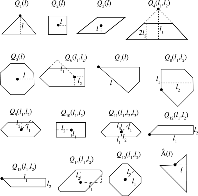
Table 5: Polygonal shapes encountered in the text. All of these are convex with the exception of A^^A\widehat{\mathrm{A}}, the arrowhead.
Q1(l)[(6,1,3),(l,0,0)]Q2(l)[(4,6,0,2),(l,l,l,l)]Q3(l)[(6,7,2,3),(l,l,l,l)]Q4(l1,l2)[(6,1,2,3),(l1,0,l2,0)]Q5(l)[(0,1,,7),(l,l,,l)]Q6(l1,l2)[(5,6,0,2,3),(0,l2,l1,l2,0)]Q7(l)[(5,7,0,2),(0,l,l,0)]Q8(l1,l2)[(4,5,7,0,1,2),(0,0,l1,l2,l2,l1)]Q9(l1,l2)[(1,2,3,5,6,7),(l1,l2,l1,l1,l2,l1)]Q10(l1,l2)[(4,6,0,2),(l2,l1,l2,l1)]Q11(l1,l2,l3)[(1,2,3,5,6,7),(l1,l2,l1,l1,l2,l1)]Q12(l1,l2)[(6,0,2,3),(0,l1,l2,0)]Q13(l1,l2)[(5,6,0,2),(0,l2,l1,0)]Q14(l1,l2)[(0,1,,7),(l1,l1,l2,l2,l1,l1,l2,l2)]Q15(l1,l2)[(0,1,,7),(l1,l2,l1,l2,l1,l2,l1,l2)]A^(l)[(5,0,2),(l,l,0)][(5,0,3),(l,l,0)]missing-subexpressionmissing-subexpressionsubscript𝑄1𝑙613𝑙00missing-subexpressionmissing-subexpressionsubscript𝑄2𝑙4602𝑙𝑙𝑙𝑙missing-subexpressionmissing-subexpressionsubscript𝑄3𝑙6723𝑙𝑙𝑙𝑙missing-subexpressionmissing-subexpressionsubscript𝑄4subscript𝑙1subscript𝑙26123subscript𝑙10subscript𝑙20missing-subexpressionmissing-subexpressionsubscript𝑄5𝑙017𝑙𝑙𝑙missing-subexpressionmissing-subexpressionsubscript𝑄6subscript𝑙1subscript𝑙2560230subscript𝑙2subscript𝑙1subscript𝑙20missing-subexpressionmissing-subexpressionsubscript𝑄7𝑙57020𝑙𝑙0missing-subexpressionmissing-subexpressionsubscript𝑄8subscript𝑙1subscript𝑙245701200subscript𝑙1subscript𝑙2subscript𝑙2subscript𝑙1missing-subexpressionmissing-subexpressionsubscript𝑄9subscript𝑙1subscript𝑙2123567subscript𝑙1subscript𝑙2subscript𝑙1subscript𝑙1subscript𝑙2subscript𝑙1missing-subexpressionmissing-subexpressionsubscript𝑄10subscript𝑙1subscript𝑙24602subscript𝑙2subscript𝑙1subscript𝑙2subscript𝑙1missing-subexpressionmissing-subexpressionsubscript𝑄11subscript𝑙1subscript𝑙2subscript𝑙3123567subscript𝑙1subscript𝑙2subscript𝑙1subscript𝑙1subscript𝑙2subscript𝑙1missing-subexpressionmissing-subexpressionsubscript𝑄12subscript𝑙1subscript𝑙260230subscript𝑙1subscript𝑙20missing-subexpressionmissing-subexpressionsubscript𝑄13subscript𝑙1subscript𝑙256020subscript𝑙2subscript𝑙10missing-subexpressionmissing-subexpressionsubscript𝑄14subscript𝑙1subscript𝑙2017subscript𝑙1subscript𝑙1subscript𝑙2subscript𝑙2subscript𝑙1subscript𝑙1subscript𝑙2subscript𝑙2missing-subexpressionmissing-subexpressionsubscript𝑄15subscript𝑙1subscript𝑙2017subscript𝑙1subscript𝑙2subscript𝑙1subscript𝑙2subscript𝑙1subscript𝑙2subscript𝑙1subscript𝑙2missing-subexpressionmissing-subexpression^A𝑙502𝑙𝑙0503𝑙𝑙0\begin{array}[]{|c|c|}\hline\cr Q_{1}(l)&[(6,1,3),(l,0,0)]\\ \hline\cr Q_{2}(l)&[(4,6,0,2),(l,l,l,l)]\\ \hline\cr Q_{3}(l)&[(6,7,2,3),(l,l,l,l)]\\ \hline\cr Q_{4}(l_{1},l_{2})&[(6,1,2,3),(l_{1},0,-l_{2},0)]\\ \hline\cr Q_{5}(l)&[(0,1,\ldots,7),(l,l,\ldots,l)]\\ \hline\cr Q_{6}(l_{1},l_{2})&[(5,6,0,2,3),(0,l_{2},l_{1},l_{2},0)]\\ \hline\cr Q_{7}(l)&[(5,7,0,2),(0,l,l,0)]\\ \hline\cr Q_{8}(l_{1},l_{2})&[(4,5,7,0,1,2),(0,0,l_{1},l_{2},l_{2},l_{1})]\\ \hline\cr Q_{9}(l_{1},l_{2})&[(1,2,3,5,6,7),(l_{1},l_{2},l_{1},l_{1},l_{2},l_{1})]\\ \hline\cr Q_{10}(l_{1},l_{2})&[(4,6,0,2),(l_{2},l_{1},l_{2},l_{1})]\\ \hline\cr Q_{11}(l_{1},l_{2},l_{3})&[(1,2,3,5,6,7),(l_{1},l_{2},l_{1},l_{1},l_{2},l_{1})]\\ \hline\cr Q_{12}(l_{1},l_{2})&[(6,0,2,3),(0,l_{1},l_{2},0)]\\ \hline\cr Q_{13}(l_{1},l_{2})&[(5,6,0,2),(0,l_{2},l_{1},0)]\\ \hline\cr Q_{14}(l_{1},l_{2})&[(0,1,\ldots,7),(l_{1},l_{1},l_{2},l_{2},l_{1},l_{1},l_{2},l_{2})]\\ \hline\cr Q_{15}(l_{1},l_{2})&[(0,1,\ldots,7),(l_{1},l_{2},l_{1},l_{2},l_{1},l_{2},l_{1},l_{2})]\\ \hline\cr\widehat{\mathrm{A}}(l)&[(5,0,2),(l,l,0)]\cup[(5,0,3),(l,l,0)]\\ \hline\cr\end{array}
Refer to caption
Figure 28: Polygonal shapes listed in Table 5, with anchor points emphasized.

Appendix B: Tiling plans

Key:

  • Heading, ‘Parent dressed domain’:    PWI for constructing orbits by direct iteration.

  • Heading, ‘Tiling domains’:   spans of listed source tiles, expressed in terms of the representative polygons of Appendix A.

  • Col. 1, ‘Tile’:   name of source tile whose orbit is to be calculated.

  • Cols 2, 3, ‘Q#subscript𝑄#Q_{\#}’, ‘Parameters’:   source tile representative polygon and parameters (see Appendix A).

  • Cols 4, 5, ‘𝚁#subscript𝚁#\mathtt{R}_{\#}’, ‘Translation’:  index n𝑛n of rotation 𝚁nsubscript𝚁𝑛\mathtt{R}_{n}, and translation (dx,dy)subscript𝑑𝑥subscript𝑑𝑦(d_{x},d_{y}) of source tile relative to representative polygon.

  • Col 6, 7: ‘tile’, ‘𝚁#subscript𝚁#\mathtt{R}_{\#}’:   destination tile and index n𝑛n of net rotation 𝚁nsubscript𝚁𝑛\mathtt{R}_{n} relative to source tile. These specify the net isometry to be verified by direct iteration.

TILING PLAN 1 :,sI0,1=(β+β3,αβ)Parent dressed domain:^(1,s)Tiling domain:B=𝚃(2β2+βs,4βs)𝚁2Q1(2β2βs)Data for Direct IterationSource PolygonInitial PlacementDestinationTileQ#Parameters𝚁#TranslationTile𝚁#B112αβ3+βs7(0,24β3)B1B6B274β2+αs6(0,1412α+αs)B2B5B36αβ3+βs,αβs5(0,1210α)B3B6B472βαs1(2β+αs,1210α)B4B7B51αβ2βs2(αβ2+βs,1411αs)B5B0Π12s0(s,s)Π12Π252βs0(2βs,s)Π25Π33β+s0(1s,βs)Π34Π45αβs0(αβs,αβs)Π43Π55αβs0(αβ2s,αs)Π53Π672βαs5(4β(2+α)s,2β2s)Π60Π71αβ2βs6(6+5αωs,αs)Π70Π852αβ2+s0(2αβ2s,108αs)Π83Π910αβs,2αβ2+s1(βs,3βs)Π94missing-subexpressionmissing-subexpressionformulae-sequenceTILING PLAN 1 :superscript𝑠subscript𝐼01𝛽superscript𝛽3𝛼𝛽missing-subexpressionmissing-subexpressionmissing-subexpressionParent dressed domain:^1𝑠missing-subexpressionTiling domain:superscriptBsubscript𝚃2superscript𝛽2𝛽𝑠4𝛽𝑠subscript𝚁2subscript𝑄12superscript𝛽2𝛽𝑠missing-subexpressionData for Direct Iterationmissing-subexpressionmissing-subexpressionmissing-subexpressionmissing-subexpressionmissing-subexpressionmissing-subexpressionmissing-subexpressionSource PolygonInitial PlacementDestinationmissing-subexpressionmissing-subexpressionmissing-subexpressionmissing-subexpressionmissing-subexpressionmissing-subexpressionmissing-subexpressionTilesubscript𝑄#Parameterssubscript𝚁#TranslationTilesubscript𝚁#missing-subexpressionmissing-subexpressionmissing-subexpressionmissing-subexpressionmissing-subexpressionmissing-subexpressionmissing-subexpressionmissing-subexpressionmissing-subexpressionmissing-subexpressionmissing-subexpressionmissing-subexpressionmissing-subexpressionmissing-subexpressionsubscriptsuperscript𝐵112𝛼superscript𝛽3𝛽𝑠7024superscript𝛽3subscriptsuperscript𝐵1superscript𝐵6missing-subexpressionmissing-subexpressionmissing-subexpressionmissing-subexpressionmissing-subexpressionmissing-subexpressionmissing-subexpressionsubscriptsuperscript𝐵274superscript𝛽2𝛼𝑠601412𝛼𝛼𝑠subscriptsuperscript𝐵2superscript𝐵5missing-subexpressionmissing-subexpressionmissing-subexpressionmissing-subexpressionmissing-subexpressionmissing-subexpressionmissing-subexpressionsubscriptsuperscript𝐵36𝛼superscript𝛽3𝛽𝑠𝛼𝛽𝑠501210𝛼subscriptsuperscript𝐵3superscript𝐵6missing-subexpressionmissing-subexpressionmissing-subexpressionmissing-subexpressionmissing-subexpressionmissing-subexpressionmissing-subexpressionsubscriptsuperscript𝐵472𝛽𝛼𝑠12𝛽𝛼𝑠1210𝛼subscriptsuperscript𝐵4superscript𝐵7missing-subexpressionmissing-subexpressionmissing-subexpressionmissing-subexpressionmissing-subexpressionmissing-subexpressionmissing-subexpressionsubscriptsuperscript𝐵51𝛼superscript𝛽2𝛽𝑠2𝛼superscript𝛽2𝛽𝑠1411𝛼𝑠subscriptsuperscript𝐵5superscript𝐵0missing-subexpressionmissing-subexpressionmissing-subexpressionmissing-subexpressionmissing-subexpressionmissing-subexpressionmissing-subexpressionmissing-subexpressionmissing-subexpressionmissing-subexpressionmissing-subexpressionmissing-subexpressionmissing-subexpressionmissing-subexpressionsubscriptΠ12𝑠0𝑠𝑠subscriptΠ12missing-subexpressionmissing-subexpressionmissing-subexpressionmissing-subexpressionmissing-subexpressionmissing-subexpressionmissing-subexpressionsubscriptΠ252𝛽𝑠02𝛽𝑠𝑠subscriptΠ25missing-subexpressionmissing-subexpressionmissing-subexpressionmissing-subexpressionmissing-subexpressionmissing-subexpressionmissing-subexpressionsubscriptΠ33𝛽𝑠01𝑠𝛽𝑠subscriptΠ34missing-subexpressionmissing-subexpressionmissing-subexpressionmissing-subexpressionmissing-subexpressionmissing-subexpressionmissing-subexpressionsubscriptΠ45𝛼𝛽𝑠0𝛼𝛽𝑠𝛼𝛽𝑠subscriptΠ43missing-subexpressionmissing-subexpressionmissing-subexpressionmissing-subexpressionmissing-subexpressionmissing-subexpressionmissing-subexpressionsubscriptΠ55𝛼𝛽𝑠0𝛼superscript𝛽2𝑠𝛼𝑠subscriptΠ53missing-subexpressionmissing-subexpressionmissing-subexpressionmissing-subexpressionmissing-subexpressionmissing-subexpressionmissing-subexpressionsubscriptΠ672𝛽𝛼𝑠54𝛽2𝛼𝑠2𝛽2𝑠subscriptΠ60missing-subexpressionmissing-subexpressionmissing-subexpressionmissing-subexpressionmissing-subexpressionmissing-subexpressionmissing-subexpressionsubscriptΠ71𝛼superscript𝛽2𝛽𝑠665𝛼𝜔𝑠𝛼𝑠subscriptΠ70missing-subexpressionmissing-subexpressionmissing-subexpressionmissing-subexpressionmissing-subexpressionmissing-subexpressionmissing-subexpressionsubscriptΠ852𝛼superscript𝛽2𝑠02𝛼superscript𝛽2𝑠108𝛼𝑠subscriptΠ83missing-subexpressionmissing-subexpressionmissing-subexpressionmissing-subexpressionmissing-subexpressionmissing-subexpressionmissing-subexpressionsubscriptΠ910𝛼𝛽𝑠2𝛼superscript𝛽2𝑠1𝛽𝑠3𝛽𝑠subscriptΠ94\begin{array}[]{|c|}\hline\cr\\ \mbox{TILING PLAN 1 :}\quad{\mathcal{B}}\rightarrow{\mathcal{B}}^{*},\quad s\in I_{0,-1}=(\beta+\beta^{3},\alpha\beta)\\ \\ \hline\cr\begin{array}[]{l}\\ \mbox{Parent dressed domain:}\qquad\widehat{{\mathcal{B}}}(1,s)\\ \\ \mbox{Tiling domain:}\quad{\rm B}^{*}={\tt T}_{(-2\beta^{2}+\beta s,-4\beta-s)}\,\,{\tt R}_{2}\,\,Q_{1}(2\beta^{2}-\beta s)\\ \end{array}\\ \\ \mbox{\sc Data for Direct Iteration}\\ \begin{array}[]{c|c|c|c|c|c|c}\hline\cr\lx@intercol\hfil\mbox{Source Polygon}\hfil\lx@intercol\vrule\lx@intercol&\vrule\lx@intercol\hfil\mbox{Initial Placement}\hfil\lx@intercol\vrule\lx@intercol&\vrule\lx@intercol\hfil\mbox{Destination}\hfil\lx@intercol\\ \hline\cr\mbox{Tile}&Q_{\#}&\mbox{Parameters}&{\tt R}_{\#}&\mbox{Translation}&\mbox{Tile}&{\tt R}_{\#}\\ \hline\cr\hline\cr B^{*}_{1}&1&-2\alpha\beta^{3}+\beta s&7&(0,-2-4\beta^{3})&B^{*}_{1}\oslash B^{*}&6\\ \hline\cr B^{*}_{2}&7&-4\beta^{2}+\alpha s&6&(0,14-12\alpha+\alpha s)&B^{*}_{2}\oslash B^{*}&5\\ \hline\cr B^{*}_{3}&6&-\alpha\beta^{3}+\beta s,\alpha\beta-\ s&5&(0,12-10\alpha)&B^{*}_{3}\oslash B^{*}&6\\ \hline\cr B^{*}_{4}&7&2\beta-\alpha s&1&(-2\beta+\alpha s,12-10\alpha)&B^{*}_{4}\oslash B^{*}&7\\ \hline\cr B^{*}_{5}&1&\alpha\beta^{2}-\beta s&2&(-\alpha\beta^{2}+\beta s,14-11\alpha-s)&B^{*}_{5}\oslash B^{*}&0\\ \hline\cr\hline\cr\Pi_{1}&2&s&0&(-s,-s)&\Pi_{1}&2\\ \hline\cr\Pi_{2}&5&2\beta-\ s&0&(-2\beta-s,-s)&\Pi_{2}&5\\ \hline\cr\Pi_{3}&3&-\beta+s&0&(-1-s,\beta-s)&\Pi_{3}&4\\ \hline\cr\Pi_{4}&5&\alpha\beta-s&0&(-\alpha\beta-s,-\alpha\beta-s)&\Pi_{4}&3\\ \hline\cr\Pi_{5}&5&\alpha\beta-s&0&(\alpha\beta^{2}-s,-\alpha-s)&\Pi_{5}&3\\ \hline\cr\Pi_{6}&7&2\beta-\alpha s&5&(4\beta-(2+\alpha)s,-2\beta-2s)&\Pi_{6}&0\\ \hline\cr\Pi_{7}&1&\alpha\beta^{2}-\beta s&6&(-6+5\alpha-\omega s,-\alpha-s)&\Pi_{7}&0\\ \hline\cr\Pi_{8}&5&-2\alpha\beta^{2}+s&0&(2\alpha\beta^{2}-s,10-8\alpha-s)&\Pi_{8}&3\\ \hline\cr\Pi_{9}&10&\alpha\beta-s,-2\alpha\beta^{2}+s&1&(\beta-s,-3\beta-s)&\Pi_{9}&4\\ \end{array}\\ \hline\cr\end{array}
TILING PLAN 2 :,s=βParent dressed domain:^(1,s)Tiling domains:B=𝚃(β,12α)𝚁2Q1(β)B=𝚃(4β,2αβ2)𝚁7Q1(β3)Data for Direct IterationSource PolygonInitial PlacementDestinationTileQ#Parameters𝚁#TranslationTile𝚁#B11β25(0,4β)B1B2B27αβ3(0,23α)B2B3B11β42(13+8α,1511α)B1B2B27αβ30(3αβ,2αβ2)B2B3Π12β0(β,β)Π12Π25β0(3β,βΠ25Π35β30(119α,β)Π35Π45β20(1,1)Π43\begin{array}[]{|c|}\hline\cr\\ \mbox{TILING PLAN 2 :}\quad{\mathcal{B}}\rightarrow{\mathcal{B}}^{*},\quad s=\beta\\ \\ \hline\cr\begin{array}[]{l}\\ \mbox{Parent dressed domain:}\qquad\widehat{{\mathcal{B}}}(1,s)\\ \\ \mbox{Tiling domains:}\quad\begin{array}[]{l}{\rm B}^{*}={\tt T}_{(-\beta,1-2\alpha)}\,\,{\tt R}_{2}\,\,Q_{1}(\beta)\\ {\rm B}^{\dagger}={\tt T}_{(-4\beta,-2\alpha\beta^{2})}\,\,{\tt R}_{7}\,\,{Q}_{1}(\beta^{3})\end{array}\end{array}\\ \\ \mbox{\sc Data for Direct Iteration}\\ \begin{array}[]{c|c|c|c|c|c|c}\hline\cr\lx@intercol\hfil\mbox{Source Polygon}\hfil\lx@intercol\vrule\lx@intercol&\vrule\lx@intercol\hfil\mbox{Initial Placement}\hfil\lx@intercol\vrule\lx@intercol&\vrule\lx@intercol\hfil\mbox{Destination}\hfil\lx@intercol\\ \hline\cr\mbox{Tile}&Q_{\#}&\mbox{Parameters}&{\tt R}_{\#}&\mbox{Translation}&\mbox{Tile}&{\tt R}_{\#}\\ \hline\cr\hline\cr B^{*}_{1}&1&\beta^{2}&5&(0,-4\beta)&B^{*}_{1}\oslash B^{*}&2\\ \hline\cr B^{*}_{2}&7&\alpha\beta&3&(0,2-3\alpha)&B^{*}_{2}\oslash B^{*}&3\\ \hline\cr B^{\dagger}_{1}&1&\beta^{4}&2&(-13+8\alpha,15-11\alpha)&B^{\dagger}_{1}\oslash B^{\dagger}&2\\ \hline\cr B^{\dagger}_{2}&7&\alpha\beta^{3}&0&(-3\alpha\beta,-2\alpha\beta^{2})&B^{\dagger}_{2}\oslash B^{\dagger}&3\\ \hline\cr\hline\cr\Pi_{1}&2&\beta&0&\left(-\beta,-\beta\right)&\Pi_{1}&2\\ \hline\cr\Pi_{2}&5&\beta&0&(-3\beta,-\beta&\Pi_{2}&5\\ \hline\cr\Pi_{3}&5&\beta^{3}&0&(11-9\alpha,-\beta)&\Pi_{3}&5\\ \hline\cr\Pi_{4}&5&\beta^{2}&0&(-1,-1)&\Pi_{4}&3\end{array}\\ \hline\cr\end{array}
TILING PLAN 3 :𝒫,s(0,αβ2)Parent dressed domain:^(1,s)Tiling domains:P=𝚃(2+βs,s)Q6(2βs,s)A=𝚃(2β2αβs,2αβ2s)A^(2β2αs)Data for Direct IterationSource PolygonInitial PlacementDestinationTileQ#Parameters𝚁#TranslationTile𝚁#P02s0(s,s)P0P2P19βs,s0(αs,s)P1P4P27αs1(2βαωs,2s)P2P7P31βs3(2β2s,2s)P5P6P43s3(2βs,s)P4P5P54αβ2βs,αβ2ωs4(αβs,αβ2+βs)P3P4P63s0(2β2s,s)P6P3Pin122β2αs,2s0(2β2αβs,2s)A2A0A11αβωs2(αβ+βs,αs)A1A5A2132β2αs,2s5(2β2αβs,2αβ2s)PinP3A31αβ2ωs4(αβs,α+βs)A3A1Π5αβs0(αβs,αβs)Π3missing-subexpressionmissing-subexpressionformulae-sequenceTILING PLAN 3 :𝒫𝑠0𝛼superscript𝛽2missing-subexpressionmissing-subexpressionmissing-subexpressionParent dressed domain:^1𝑠missing-subexpressionTiling domains:Psubscript𝚃2𝛽𝑠𝑠subscript𝑄62𝛽𝑠𝑠Asubscript𝚃2superscript𝛽2𝛼𝛽𝑠2𝛼𝛽2𝑠^A2superscript𝛽2𝛼𝑠missing-subexpressionData for Direct Iterationmissing-subexpressionmissing-subexpressionmissing-subexpressionmissing-subexpressionmissing-subexpressionmissing-subexpressionmissing-subexpressionSource PolygonInitial PlacementDestinationmissing-subexpressionmissing-subexpressionmissing-subexpressionmissing-subexpressionmissing-subexpressionmissing-subexpressionmissing-subexpressionTilesubscript𝑄#Parameterssubscript𝚁#TranslationTilesubscript𝚁#missing-subexpressionmissing-subexpressionmissing-subexpressionmissing-subexpressionmissing-subexpressionmissing-subexpressionmissing-subexpressionmissing-subexpressionmissing-subexpressionmissing-subexpressionmissing-subexpressionmissing-subexpressionmissing-subexpressionmissing-subexpressionsubscript𝑃02𝑠0𝑠𝑠subscript𝑃0𝑃2missing-subexpressionmissing-subexpressionmissing-subexpressionmissing-subexpressionmissing-subexpressionmissing-subexpressionmissing-subexpressionsubscript𝑃19𝛽𝑠𝑠0𝛼𝑠𝑠subscript𝑃1𝑃4missing-subexpressionmissing-subexpressionmissing-subexpressionmissing-subexpressionmissing-subexpressionmissing-subexpressionmissing-subexpressionsubscript𝑃27𝛼𝑠12𝛽𝛼𝜔𝑠2𝑠subscript𝑃2𝑃7missing-subexpressionmissing-subexpressionmissing-subexpressionmissing-subexpressionmissing-subexpressionmissing-subexpressionmissing-subexpressionsubscript𝑃31𝛽𝑠32𝛽2𝑠2𝑠subscript𝑃5𝑃6missing-subexpressionmissing-subexpressionmissing-subexpressionmissing-subexpressionmissing-subexpressionmissing-subexpressionmissing-subexpressionsubscript𝑃43𝑠32𝛽𝑠𝑠subscript𝑃4𝑃5missing-subexpressionmissing-subexpressionmissing-subexpressionmissing-subexpressionmissing-subexpressionmissing-subexpressionmissing-subexpressionsubscript𝑃54𝛼superscript𝛽2𝛽𝑠𝛼superscript𝛽2𝜔𝑠4𝛼𝛽𝑠𝛼superscript𝛽2𝛽𝑠subscript𝑃3𝑃4missing-subexpressionmissing-subexpressionmissing-subexpressionmissing-subexpressionmissing-subexpressionmissing-subexpressionmissing-subexpressionsubscript𝑃63𝑠02superscript𝛽2𝑠𝑠subscript𝑃6𝑃3missing-subexpressionmissing-subexpressionmissing-subexpressionmissing-subexpressionmissing-subexpressionmissing-subexpressionmissing-subexpressionsubscript𝑃in122superscript𝛽2𝛼𝑠2𝑠02superscript𝛽2𝛼𝛽𝑠2𝑠subscript𝐴2A0missing-subexpressionmissing-subexpressionmissing-subexpressionmissing-subexpressionmissing-subexpressionmissing-subexpressionmissing-subexpressionmissing-subexpressionmissing-subexpressionmissing-subexpressionmissing-subexpressionmissing-subexpressionmissing-subexpressionmissing-subexpressionsubscript𝐴11𝛼𝛽𝜔𝑠2𝛼𝛽𝛽𝑠𝛼𝑠subscript𝐴1A5missing-subexpressionmissing-subexpressionmissing-subexpressionmissing-subexpressionmissing-subexpressionmissing-subexpressionmissing-subexpressionsubscript𝐴2132superscript𝛽2𝛼𝑠2𝑠52superscript𝛽2𝛼𝛽𝑠2𝛼𝛽2𝑠subscript𝑃in𝑃3missing-subexpressionmissing-subexpressionmissing-subexpressionmissing-subexpressionmissing-subexpressionmissing-subexpressionmissing-subexpressionsubscript𝐴31𝛼superscript𝛽2𝜔𝑠4𝛼𝛽𝑠𝛼𝛽𝑠subscript𝐴3A1missing-subexpressionmissing-subexpressionmissing-subexpressionmissing-subexpressionmissing-subexpressionmissing-subexpressionmissing-subexpressionmissing-subexpressionmissing-subexpressionmissing-subexpressionmissing-subexpressionmissing-subexpressionmissing-subexpressionmissing-subexpressionΠ5𝛼𝛽𝑠0𝛼𝛽𝑠𝛼𝛽𝑠Π3\begin{array}[]{|c|}\hline\cr\\ \mbox{TILING PLAN 3 :}\quad{\mathcal{B}}\rightarrow{\mathcal{P}},\quad s\in(0,\alpha\beta^{2})\\ \\ \hline\cr\begin{array}[]{l}\\ \mbox{Parent dressed domain:}\qquad\widehat{{\mathcal{B}}}(1,s)\\ \\ \mbox{Tiling domains:}\quad\begin{array}[]{l}{\rm P}={\tt T}_{(-2+\beta s,-s)}\,\,{Q}_{6}(2-\beta s,s)\\ {\rm A}={\tt T}_{(-2\beta^{2}-\alpha\beta s,-2\alpha\beta-2s)}\,\,\widehat{\rm A}(2\beta^{2}-\alpha s)\end{array}\par\end{array}\\ \\ \mbox{\sc Data for Direct Iteration}\\ \begin{array}[]{c|c|c|c|c|c|c}\hline\cr\lx@intercol\hfil\mbox{Source Polygon}\hfil\lx@intercol\vrule\lx@intercol&\vrule\lx@intercol\hfil\mbox{Initial Placement}\hfil\lx@intercol\vrule\lx@intercol&\vrule\lx@intercol\hfil\mbox{Destination}\hfil\lx@intercol\\ \hline\cr\mbox{Tile}&Q_{\#}&\mbox{Parameters}&{\tt R}_{\#}&\mbox{Translation}&\mbox{Tile}&{\tt R}_{\#}\\ \hline\cr\hline\cr P_{0}&2&s&0&(-s,-s)&P_{0}\oslash P&2\\ \hline\cr P_{1}&9&\beta-s,s&0&(-\alpha-s,-s)&P_{1}\oslash P&4\\ \hline\cr P_{2}&7&\alpha s&1&(-2\beta-\alpha\omega s,-2s)&P_{2}\oslash P&7\\ \hline\cr P_{3}&1&\beta s&3&(-2\beta-2s,-2s)&P_{5}\oslash P&6\\ \hline\cr P_{4}&3&s&3&(-2\beta-s,-s)&P_{4}\oslash P&5\\ \hline\cr P_{5}&4&\alpha\beta^{2}-\beta s,\alpha\beta^{2}-\omega s&4&(-\alpha\beta-s,-\alpha\beta^{2}+\beta s)&P_{3}\oslash P&4\\ \hline\cr P_{6}&3&s&0&(-2\beta^{2}-s,-s)&P_{6}\oslash P&3\\ \hline\cr P_{\rm in}&12&2\beta^{2}-\alpha\ s,2s&0&(-2\beta^{2}-\alpha\beta s,-2s)&A_{2}\oslash{\rm A}&0\\ \hline\cr\hline\cr A_{1}&1&\alpha\beta-\omega s&2&(-\alpha\beta+\beta s,-\alpha-s)&A_{1}\oslash{\rm A}&5\\ \hline\cr A_{2}&13&2\beta^{2}-\alpha s,2s&5&(-2\beta^{2}-\alpha\beta s,-2\alpha\beta-2s)&P_{\rm in}\oslash P&3\\ \hline\cr A_{3}&1&\alpha\beta^{2}-\omega s&4&(-\alpha\beta-s,-\alpha+\beta s)&A_{3}\oslash{\rm A}&1\\ \hline\cr\hline\cr\Pi&5&\alpha\beta-s&0&(-\alpha\beta-s,-\alpha\beta-s)&\Pi&3\end{array}\\ \hline\cr\end{array}
TILING PLAN 4 : 𝒫,s=β2Parent dressed domain:𝒫^(α,β2)Tiling domains:B=𝚃(αβ,0)𝚁4Q1(β2)B=𝚃(αβ2,2β3)Q1(β5)Data for Direct IterationSource PolygonInitial PlacementDestinationTileQ#Parameters𝚁#TranslationTile𝚁#B11β31(3β2,β2)B1B6B27αβ20(5+3α,β2)B2B5B11β55(β5αβ2,β2)B1B6B27αβ44(3β3,β2)B2B5Π12β20(0,0)Π12Π29αβ2,β20(α,0))Π24Π31β33(1,β2)Π30Π45β20(2β,0)Π45Π55β20(2β2,0)Π53Π65β40(αβ4αβ,0)Π63\begin{array}[]{|c|}\hline\cr\\ \mbox{TILING PLAN 4 : }\quad{\mathcal{P}}\rightarrow{\mathcal{B}},\quad s=\beta^{2}\\ \\ \hline\cr\\ \mbox{Parent dressed domain:}\qquad\widehat{{\mathcal{P}}}(\alpha,\beta^{2})\\ \\ \mbox{Tiling domains:}\quad\begin{array}[]{l}{\rm B}^{*}={\tt T}_{(-\alpha\beta,0)}{\tt R}_{4}Q_{1}(\beta^{2})\\ {\rm B}^{\dagger}={\tt T}_{(-\alpha\beta^{2},-2\beta^{3})}Q_{1}(\beta^{5})\end{array}\\ \\ \mbox{\sc Data for Direct Iteration}\\ \begin{array}[]{c|c|c|c|c|c|c}\hline\cr\lx@intercol\hfil\mbox{Source Polygon}\hfil\lx@intercol\vrule\lx@intercol&\vrule\lx@intercol\hfil\mbox{Initial Placement}\hfil\lx@intercol\vrule\lx@intercol&\vrule\lx@intercol\hfil\mbox{Destination}\hfil\lx@intercol\\ \hline\cr\mbox{Tile}&Q_{\#}&\mbox{Parameters}&{\tt R}_{\#}&\mbox{Translation}&\mbox{Tile}&{\tt R}_{\#}\\ \hline\cr\hline\cr B^{*}_{1}&1&\beta^{3}&1&(-3\beta^{2},\beta^{2})&B^{*}_{1}\oslash B^{*}&6\\ \hline\cr B^{*}_{2}&7&\alpha\beta^{2}&0&(-5+3\alpha,\beta^{2})&B^{*}_{2}\oslash B^{*}&5\\ \hline\cr B^{\dagger}_{1}&1&\beta^{5}&5&(-\beta^{5}-\alpha\beta^{2},-\beta^{2})&B^{\dagger}_{1}\oslash B^{\dagger}&6\\ \hline\cr B^{\dagger}_{2}&7&\alpha\beta^{4}&4&(-3\beta^{3},-\beta^{2})&B^{\dagger}_{2}\oslash B^{\dagger}&5\\ \hline\cr\Pi_{1}&2&\beta^{2}&0&(0,0)&\Pi_{1}&2\\ \hline\cr\Pi_{2}&9&\alpha\beta^{2},\beta^{2}&0&(-\alpha,0))&\Pi_{2}&4\\ \hline\cr\Pi_{3}&1&\beta^{3}&3&(-1,-\beta^{2})&\Pi_{3}&0\\ \hline\cr\Pi_{4}&5&\beta^{2}&0&(-2\beta,0)&\Pi_{4}&5\\ \hline\cr\Pi_{5}&5&\beta^{2}&0&(-2\beta^{2},0)&\Pi_{5}&3\\ \hline\cr\Pi_{6}&5&\beta^{4}&0&(\alpha\beta^{4}-\alpha\beta,0)&\Pi_{6}&3\end{array}\\ \hline\cr\end{array}
TILING PLAN 5 :𝒯,s(β,β+β4]Parent dressed domain:^(1,s)Tiling domains:T=𝚃(αβ+βs,αs)𝚁2Q1(αββs)A=𝚃(2βαβs,2s)A^(2βαs)Data for Direct IterationSource PolygonInitial PlacementDestinationTileQ#Parameters𝚁#TranslationTile𝚁#T11βs5(0,2β2s)T1T2T272ωs3(2β2s,2α+αs)T2T3T33β+s1(βs,76αs)T3T1T442β2βs,2αβωs2(2β2+βs,4βs)T4T0Tin132βαs,2β+2s2(2β2s,4βαβs)A2A3A11αωs7(2s,2s)A1A3A2122βαs,2β+2s0(2βαβs,2s)TinT6A312αβωs5(2s,2β)A^3A7Π12s0(s,s)Π12Π252βs0(2βs,s)Π25Π33β+s0(1s,βs)Π34missing-subexpressionmissing-subexpressionformulae-sequenceTILING PLAN 5 :subscript𝒯𝑠𝛽𝛽superscript𝛽4missing-subexpressionmissing-subexpressionmissing-subexpressionParent dressed domain:^1𝑠missing-subexpressionTiling domains:subscriptTsubscript𝚃𝛼𝛽𝛽𝑠𝛼𝑠subscript𝚁2subscript𝑄1𝛼𝛽𝛽𝑠Asubscript𝚃2𝛽𝛼𝛽𝑠2𝑠^𝐴2𝛽𝛼𝑠missing-subexpressionData for Direct Iterationmissing-subexpressionmissing-subexpressionmissing-subexpressionmissing-subexpressionmissing-subexpressionmissing-subexpressionmissing-subexpressionSource PolygonInitial PlacementDestinationmissing-subexpressionmissing-subexpressionmissing-subexpressionmissing-subexpressionmissing-subexpressionmissing-subexpressionmissing-subexpressionTilesubscript𝑄#Parameterssubscript𝚁#TranslationTilesubscript𝚁#missing-subexpressionmissing-subexpressionmissing-subexpressionmissing-subexpressionmissing-subexpressionmissing-subexpressionmissing-subexpressionmissing-subexpressionmissing-subexpressionmissing-subexpressionmissing-subexpressionmissing-subexpressionmissing-subexpressionmissing-subexpressionsubscriptsuperscript𝑇11𝛽𝑠502𝛽2𝑠subscriptsuperscript𝑇1subscriptT2missing-subexpressionmissing-subexpressionmissing-subexpressionmissing-subexpressionmissing-subexpressionmissing-subexpressionmissing-subexpressionsubscriptsuperscript𝑇272𝜔𝑠32𝛽2𝑠2𝛼𝛼𝑠subscriptsuperscript𝑇2subscriptT3missing-subexpressionmissing-subexpressionmissing-subexpressionmissing-subexpressionmissing-subexpressionmissing-subexpressionmissing-subexpressionsubscriptsuperscript𝑇33𝛽𝑠1𝛽𝑠76𝛼𝑠subscriptsuperscript𝑇3subscriptT1missing-subexpressionmissing-subexpressionmissing-subexpressionmissing-subexpressionmissing-subexpressionmissing-subexpressionmissing-subexpressionsubscriptsuperscript𝑇442superscript𝛽2𝛽𝑠2𝛼𝛽𝜔𝑠22superscript𝛽2𝛽𝑠4𝛽𝑠subscriptsuperscript𝑇4subscriptT0missing-subexpressionmissing-subexpressionmissing-subexpressionmissing-subexpressionmissing-subexpressionmissing-subexpressionmissing-subexpressionsubscriptsuperscript𝑇in132𝛽𝛼𝑠2𝛽2𝑠22𝛽2𝑠4𝛽𝛼𝛽𝑠subscript𝐴2A3missing-subexpressionmissing-subexpressionmissing-subexpressionmissing-subexpressionmissing-subexpressionmissing-subexpressionmissing-subexpressionsubscript𝐴11𝛼𝜔𝑠72𝑠2𝑠subscript𝐴1A3missing-subexpressionmissing-subexpressionmissing-subexpressionmissing-subexpressionmissing-subexpressionmissing-subexpressionmissing-subexpressionsubscript𝐴2122𝛽𝛼𝑠2𝛽2𝑠02𝛽𝛼𝛽𝑠2𝑠subscriptsuperscript𝑇insubscriptT6missing-subexpressionmissing-subexpressionmissing-subexpressionmissing-subexpressionmissing-subexpressionmissing-subexpressionmissing-subexpressionsubscript𝐴312𝛼𝛽𝜔𝑠52𝑠2𝛽subscript^𝐴3A7missing-subexpressionmissing-subexpressionmissing-subexpressionmissing-subexpressionmissing-subexpressionmissing-subexpressionmissing-subexpressionsubscriptΠ12𝑠0𝑠𝑠subscriptΠ12missing-subexpressionmissing-subexpressionmissing-subexpressionmissing-subexpressionmissing-subexpressionmissing-subexpressionmissing-subexpressionsubscriptΠ252𝛽𝑠02𝛽𝑠𝑠subscriptΠ25missing-subexpressionmissing-subexpressionmissing-subexpressionmissing-subexpressionmissing-subexpressionmissing-subexpressionmissing-subexpressionsubscriptΠ33𝛽𝑠01𝑠𝛽𝑠subscriptΠ34\begin{array}[]{|c|}\hline\cr\\ \mbox{TILING PLAN 5 :}\quad{\mathcal{B}}\rightarrow{\mathcal{T}}_{-},\quad s\in(\beta,\beta+\beta^{4}]\\ \\ \hline\cr\begin{array}[]{l}\\ \mbox{Parent dressed domain:}\qquad\widehat{{\mathcal{B}}}(1,s)\\ \\ \mbox{Tiling domains:}\quad\begin{array}[]{l}\mathrm{T}_{-}={\tt T}_{(-\alpha\beta+\beta s,-\alpha-s)}{\tt R}_{2}Q_{1}(\alpha\beta-\beta s)\\ \mathrm{A}={\tt T}_{(-2\beta-\alpha\beta s,-2s)}\widehat{A}(2\beta-\alpha s)\end{array}\end{array}\\ \\ \mbox{\sc Data for Direct Iteration}\\ \begin{array}[]{c|c|c|c|c|c|c}\hline\cr\lx@intercol\hfil\mbox{Source Polygon}\hfil\lx@intercol\vrule\lx@intercol&\vrule\lx@intercol\hfil\mbox{Initial Placement}\hfil\lx@intercol\vrule\lx@intercol&\vrule\lx@intercol\hfil\mbox{Destination}\hfil\lx@intercol\\ \hline\cr\mbox{Tile}&Q_{\#}&\mbox{Parameters}&{\tt R}_{\#}&\mbox{Translation}&\mbox{Tile}&{\tt R}_{\#}\\ \hline\cr\hline\cr T^{-}_{1}&1&\beta s&5&(0,-2\beta-2s)&T^{-}_{1}\oslash{\rm T}_{-}&2\\ \hline\cr T^{-}_{2}&7&2-\omega s&3&(2\beta-2s,-2\alpha+\alpha s)&T^{-}_{2}\oslash{\rm T}_{-}&3\\ \hline\cr T^{-}_{3}&3&-\beta+s&1&(\beta-s,7-6\alpha-s)&T^{-}_{3}\oslash{\rm T}_{-}&1\\ \hline\cr T^{-}_{4}&4&2\beta^{2}-\beta s,2\alpha\beta-\omega s&2&(-2\beta^{2}+\beta s,-4\beta-s)&T^{-}_{4}\oslash{\rm T}_{-}&0\\ \hline\cr T^{-}_{{\rm in}}&13&2\beta-\alpha s,-2\beta+2s&2&(2\beta-2s,-4\beta-\alpha\beta s)&A_{2}\oslash\mathrm{A}&3\\ \hline\cr A_{1}&1&\alpha-\omega s&7&(-2s,-2s)&A_{1}\oslash\mathrm{A}&3\\ \hline\cr A_{2}&12&2\beta-\alpha s,-2\beta+2s&0&(-2\beta-\alpha\beta s,-2s)&T^{-}_{{\rm in}}\oslash\mathrm{T}_{-}&6\\ \hline\cr A_{3}&1&2\alpha\beta-\omega s&5&(-2s,-2\beta)&\widehat{A}_{3}\oslash\mathrm{A}&7\\ \hline\cr\Pi_{1}&2&s&0&(-s,-s)&\Pi_{1}&2\\ \hline\cr\Pi_{2}&5&2\beta-s&0&(-2\beta-s,-s)&\Pi_{2}&5\\ \hline\cr\Pi_{3}&3&-\beta+s&0&(-1-s,\beta-s)&\Pi_{3}&4\end{array}\\ \hline\cr\end{array}
TILING PLAN 6 :𝒯+,s[ββ6,β)Parent dressed domain:^(1,s)Tiling domains:T+=𝚃(αβ+βs,αs)𝚁2Q1(αββs)A=𝚃(2β2αs,2s)𝚁3A^(2αβ2+αs)Data for Direct IterationSource PolygonInitial PlacementDestinationTileQ#Parameters𝚁#TranslationTile𝚁#T1+1βs5(0,2β2s)T1+T+2T2+7αs3(0,2βαωs)T2+T+3T3+4βs,2β+ωs7(0,2)T3+T+6T4+3βs7β2s,3+αs)T4+T+1T5+2βs1(αβ3s,10+6αs)T5+T+4T6+10βs,2β2+s7(αβ3/2s,5αβ/2s)T6+T+6T7+2βs1(s,αs)T7+T+4Tin+122αβ2+αs,2β2s3(2β2αs,2αβ2s)A2A0A112β+ωs5(2β,2s)A1A5A2132αβ2+αs,2β2s0(2β2αs,2s)Tin+T+5A31β31+ωs7(2β,2β)A3A1Π12s0(s,s)Π12Π25s0(2βs,s)Π25Π35αβs0(αβs,αβs)Π33\begin{array}[]{|c|}\hline\cr\\ \mbox{TILING PLAN 6 :}\quad{\mathcal{B}}\rightarrow{\mathcal{T}}_{+},\quad s\in[\beta-\beta^{6},\beta)\\ \\ \hline\cr\begin{array}[]{l}\\ \mbox{Parent dressed domain:}\qquad\widehat{{\mathcal{B}}}(1,s)\\ \\ \mbox{Tiling domains:}\quad\begin{array}[]{l}\mathrm{T}_{+}={\tt T}_{(-\alpha\beta+\beta s,-\alpha-s)}{\tt R}_{2}Q_{1}(\alpha\beta-\beta s)\\ \mathrm{A}={\tt T}_{(-2\beta^{2}-\alpha s,-2s)}{\tt R}_{3}\widehat{A}(-2\alpha\beta^{2}+\alpha s)\end{array}\end{array}\\ \\ \mbox{\sc Data for Direct Iteration}\\ \begin{array}[]{c|c|c|c|c|c|c}\hline\cr\lx@intercol\hfil\mbox{Source Polygon}\hfil\lx@intercol\vrule\lx@intercol&\vrule\lx@intercol\hfil\mbox{Initial Placement}\hfil\lx@intercol\vrule\lx@intercol&\vrule\lx@intercol\hfil\mbox{Destination}\hfil\lx@intercol\\ \hline\cr\mbox{Tile}&Q_{\#}&\mbox{Parameters}&{\tt R}_{\#}&\mbox{Translation}&\mbox{Tile}&{\tt R}_{\#}\\ \hline\cr\hline\cr T^{+}_{1}&1&\beta s&5&(0,-2\beta-2s)&T^{+}_{1}\oslash\mathrm{T}_{+}&2\\ \hline\cr T^{+}_{2}&7&\alpha s&3&(0,-2\beta-\alpha\omega s)&T^{+}_{2}\oslash\mathrm{T}_{+}&3\\ \hline\cr T^{+}_{3}&4&\beta s,-2\beta+\omega s&7&(0,-2)&T^{+}_{3}\oslash\mathrm{T}_{+}&6\\ \hline\cr T^{+}_{4}&3&\beta-s&7&\beta^{2}-s,-3+\alpha-s)&T^{+}_{4}\oslash\mathrm{T}_{+}&1\\ \hline\cr T^{+}_{5}&2&\beta-s&1&(\alpha\beta^{3}-s,-10+6\alpha-s)&T^{+}_{5}\oslash\mathrm{T}_{+}&4\\ \hline\cr T^{+}_{6}&10&\beta-s,-2\beta^{2}+s&7&(\alpha\beta^{3}/2-s,-5\alpha\beta/2-s)&T^{+}_{6}\oslash{\rm T}_{+}&6\\ \hline\cr T^{+}_{7}&2&\beta-s&1&(-s,-\alpha-s)&T^{+}_{7}\oslash\mathrm{T}_{+}&4\\ \hline\cr T^{+}_{\rm in}&12&-2\alpha\beta^{2}+\alpha s,2\beta-2s&3&(2\beta^{2}-\alpha s,-2\alpha\beta-2s)&A_{2}\oslash\mathrm{A}&0\\ \hline\cr A_{1}&1&-2\beta+\omega s&5&(-2\beta,-2s)&A_{1}\oslash{\rm A}&5\\ \hline\cr A_{2}&13&-2\alpha\beta^{2}+\alpha s,2\beta-2s&0&(-2\beta^{2}-\alpha s,-2s)&T^{+}_{\rm in}\oslash\mathrm{T}_{+}&5\\ \hline\cr A_{3}&1&\beta^{3}-1+\omega s&7&(-2\beta,-2\beta)&A_{3}\oslash{\rm A}&1\\ \hline\cr\Pi_{1}&2&s&0&(-s,-s)&\Pi_{1}&2\\ \hline\cr\Pi_{2}&5&s&0&(-2\beta-s,-s)&\Pi_{2}&5\\ \hline\cr\Pi_{3}&5&\alpha\beta-s&0&(-\alpha\beta-s,-\alpha\beta-s)&\Pi_{3}&3\end{array}\\ \hline\cr\end{array}
TILING PLAN 7 :𝒫𝒯,s(β2,β2+β6]Parent dressed domain:𝒫^(α,s)Tiling domains:T=𝚃(αβ,αβ2+αs)𝚁4Q1(αβ2βs)A=𝚃(2β4s,2αβ4βs)𝚁6A^(αβ5+αβ2αs)Data for Direct IterationSource PolygonInitial PlacementDestinationTileQ#Parameters𝚁#TranslationTile𝚁#T11βs1(2β2s,s)T1T6T272βαωs0(2αβ+ωs,2β2s)T2T5T342β3βs4(3β2,2β3+αs)T3T0T43β2+s0(β4αβ,β2)T4T7T54αβ3βs,β4+βωs0(αβ,β4+βαs)T5T0T63β2+s7(β4+αβ,β2)T6T1T742αβ4βs,β5+βωs4(αβ4+β,2αβ4+αs)T7T0T83β2+s0(4β4β,β2)T8T7Tin12αβ5+αβ2αs,2β2+2s0(β5+β+βs,2β2s)A2A6A11β4+βωs0(αβ2,αβ3αs)A1A5A213αβ5+αβ2αs,2β2+2s3(2β4s,2αβ4βs)TinT1A31β5+βωs2(2αβ2+αs,2β3)A3A1Π12s0(0,0)Π12Π23β2+s7(3β,β2)Π24Π39βs,s0(α,0)Π34Π41βs3(2βs,s)Π40Π552β2s0(2β2,0)Π53Π65s0(2βs,s)Π65Π752αβ3s0(2αβ3,2β3)Π73missing-subexpressionmissing-subexpressionformulae-sequenceTILING PLAN 7 :superscript𝒫subscript𝒯𝑠superscript𝛽2superscript𝛽2superscript𝛽6missing-subexpressionmissing-subexpressionmissing-subexpressionParent dressed domain:^𝒫𝛼𝑠missing-subexpressionTiling domains:subscriptTsubscript𝚃𝛼𝛽𝛼superscript𝛽2𝛼𝑠subscript𝚁4subscript𝑄1𝛼superscript𝛽2𝛽𝑠Asubscript𝚃2superscript𝛽4𝑠2𝛼superscript𝛽4𝛽𝑠subscript𝚁6^𝐴𝛼superscript𝛽5𝛼superscript𝛽2𝛼𝑠missing-subexpressionData for Direct Iterationmissing-subexpressionmissing-subexpressionmissing-subexpressionmissing-subexpressionmissing-subexpressionmissing-subexpressionmissing-subexpressionSource PolygonInitial PlacementDestinationmissing-subexpressionmissing-subexpressionmissing-subexpressionmissing-subexpressionmissing-subexpressionmissing-subexpressionmissing-subexpressionTilesubscript𝑄#Parameterssubscript𝚁#TranslationTilesubscript𝚁#missing-subexpressionmissing-subexpressionmissing-subexpressionmissing-subexpressionmissing-subexpressionmissing-subexpressionmissing-subexpressionmissing-subexpressionmissing-subexpressionmissing-subexpressionmissing-subexpressionmissing-subexpressionmissing-subexpressionmissing-subexpressionsubscriptsuperscript𝑇11𝛽𝑠12superscript𝛽2𝑠𝑠subscriptsuperscript𝑇1subscriptT6missing-subexpressionmissing-subexpressionmissing-subexpressionmissing-subexpressionmissing-subexpressionmissing-subexpressionmissing-subexpressionsubscriptsuperscript𝑇272𝛽𝛼𝜔𝑠02𝛼𝛽𝜔𝑠2superscript𝛽2𝑠subscriptsuperscript𝑇2subscriptT5missing-subexpressionmissing-subexpressionmissing-subexpressionmissing-subexpressionmissing-subexpressionmissing-subexpressionmissing-subexpressionsubscriptsuperscript𝑇342superscript𝛽3𝛽𝑠43superscript𝛽22superscript𝛽3𝛼𝑠subscriptsuperscript𝑇3subscriptT0missing-subexpressionmissing-subexpressionmissing-subexpressionmissing-subexpressionmissing-subexpressionmissing-subexpressionmissing-subexpressionsubscriptsuperscript𝑇43superscript𝛽2𝑠0superscript𝛽4𝛼𝛽superscript𝛽2subscriptsuperscript𝑇4subscriptT7missing-subexpressionmissing-subexpressionmissing-subexpressionmissing-subexpressionmissing-subexpressionmissing-subexpressionmissing-subexpressionsubscriptsuperscript𝑇54𝛼superscript𝛽3𝛽𝑠superscript𝛽4𝛽𝜔𝑠0𝛼𝛽superscript𝛽4𝛽𝛼𝑠subscriptsuperscript𝑇5subscriptT0missing-subexpressionmissing-subexpressionmissing-subexpressionmissing-subexpressionmissing-subexpressionmissing-subexpressionmissing-subexpressionsubscriptsuperscript𝑇63superscript𝛽2𝑠7superscript𝛽4𝛼𝛽superscript𝛽2subscriptsuperscript𝑇6subscriptT1missing-subexpressionmissing-subexpressionmissing-subexpressionmissing-subexpressionmissing-subexpressionmissing-subexpressionmissing-subexpressionsubscriptsuperscript𝑇742𝛼superscript𝛽4𝛽𝑠superscript𝛽5𝛽𝜔𝑠4𝛼superscript𝛽4𝛽2𝛼superscript𝛽4𝛼𝑠subscriptsuperscript𝑇7subscriptT0missing-subexpressionmissing-subexpressionmissing-subexpressionmissing-subexpressionmissing-subexpressionmissing-subexpressionmissing-subexpressionsubscriptsuperscript𝑇83superscript𝛽2𝑠04superscript𝛽4𝛽superscript𝛽2subscriptsuperscript𝑇8subscriptT7missing-subexpressionmissing-subexpressionmissing-subexpressionmissing-subexpressionmissing-subexpressionmissing-subexpressionmissing-subexpressionsubscriptsuperscript𝑇in12𝛼superscript𝛽5𝛼superscript𝛽2𝛼𝑠2superscript𝛽22𝑠0superscript𝛽5𝛽𝛽𝑠2superscript𝛽2𝑠subscript𝐴2A6missing-subexpressionmissing-subexpressionmissing-subexpressionmissing-subexpressionmissing-subexpressionmissing-subexpressionmissing-subexpressionsubscript𝐴11superscript𝛽4𝛽𝜔𝑠0𝛼superscript𝛽2𝛼superscript𝛽3𝛼𝑠subscript𝐴1A5missing-subexpressionmissing-subexpressionmissing-subexpressionmissing-subexpressionmissing-subexpressionmissing-subexpressionmissing-subexpressionsubscript𝐴213𝛼superscript𝛽5𝛼superscript𝛽2𝛼𝑠2superscript𝛽22𝑠32superscript𝛽4𝑠2𝛼superscript𝛽4𝛽𝑠subscriptsuperscript𝑇insubscriptT1missing-subexpressionmissing-subexpressionmissing-subexpressionmissing-subexpressionmissing-subexpressionmissing-subexpressionmissing-subexpressionsubscript𝐴31superscript𝛽5𝛽𝜔𝑠22𝛼superscript𝛽2𝛼𝑠2superscript𝛽3subscript𝐴3A1missing-subexpressionmissing-subexpressionmissing-subexpressionmissing-subexpressionmissing-subexpressionmissing-subexpressionmissing-subexpressionsubscriptΠ12𝑠000subscriptΠ12missing-subexpressionmissing-subexpressionmissing-subexpressionmissing-subexpressionmissing-subexpressionmissing-subexpressionmissing-subexpressionsubscriptΠ23superscript𝛽2𝑠73𝛽superscript𝛽2subscriptΠ24missing-subexpressionmissing-subexpressionmissing-subexpressionmissing-subexpressionmissing-subexpressionmissing-subexpressionmissing-subexpressionsubscriptΠ39𝛽𝑠𝑠0𝛼0subscriptΠ34missing-subexpressionmissing-subexpressionmissing-subexpressionmissing-subexpressionmissing-subexpressionmissing-subexpressionmissing-subexpressionsubscriptΠ41𝛽𝑠32𝛽𝑠𝑠subscriptΠ40missing-subexpressionmissing-subexpressionmissing-subexpressionmissing-subexpressionmissing-subexpressionmissing-subexpressionmissing-subexpressionsubscriptΠ552superscript𝛽2𝑠02superscript𝛽20subscriptΠ53missing-subexpressionmissing-subexpressionmissing-subexpressionmissing-subexpressionmissing-subexpressionmissing-subexpressionmissing-subexpressionsubscriptΠ65𝑠02𝛽𝑠𝑠subscriptΠ65missing-subexpressionmissing-subexpressionmissing-subexpressionmissing-subexpressionmissing-subexpressionmissing-subexpressionmissing-subexpressionsubscriptΠ752𝛼superscript𝛽3𝑠02𝛼superscript𝛽32superscript𝛽3subscriptΠ73\begin{array}[]{|c|}\hline\cr\\ \mbox{TILING PLAN 7 :}\quad{\mathcal{P}}^{*}\rightarrow{\mathcal{T}}_{-},\quad s\in(\beta^{2},\beta^{2}+\beta^{6}]\\ \\ \hline\cr\begin{array}[]{l}\\ \mbox{Parent dressed domain:}\qquad\widehat{{\mathcal{P}}}(\alpha,s)\\ \\ \mbox{Tiling domains:}\quad\begin{array}[]{l}\mathrm{T}_{-}={\tt T}_{(-\alpha\beta,-\alpha\beta^{2}+\alpha s)}{\tt R}_{4}Q_{1}(\alpha\beta^{2}-\beta s)\\ \mathrm{A}={\tt T}_{(-2\beta^{4}-s,-2\alpha\beta^{4}-\beta s)}{\tt R}_{6}\widehat{A}(\alpha\beta^{5}+\alpha\beta^{2}-\alpha s)\end{array}\end{array}\\ \\ \mbox{\sc Data for Direct Iteration}\\ \begin{array}[]{c|c|c|c|c|c|c}\hline\cr\lx@intercol\hfil\mbox{Source Polygon}\hfil\lx@intercol\vrule\lx@intercol&\vrule\lx@intercol\hfil\mbox{Initial Placement}\hfil\lx@intercol\vrule\lx@intercol&\vrule\lx@intercol\hfil\mbox{Destination}\hfil\lx@intercol\\ \hline\cr\mbox{Tile}&Q_{\#}&\mbox{Parameters}&{\tt R}_{\#}&\mbox{Translation}&\mbox{Tile}&{\tt R}_{\#}\\ \hline\cr\hline\cr T^{-}_{1}&1&\beta s&1&(-2\beta^{2}-s,s)&T^{-}_{1}\oslash{\rm T}_{-}&6\\ \hline\cr T^{-}_{2}&7&2\beta-\alpha\omega s&0&(-2\alpha\beta+\omega s,2\beta^{2}-s)&T^{-}_{2}\oslash{\rm T}_{-}&5\\ \hline\cr T^{-}_{3}&4&2\beta^{3}-\beta s&4&(-3\beta^{2},-2\beta^{3}+\alpha s)&T^{-}_{3}\oslash{\rm T}_{-}&0\\ \hline\cr T^{-}_{4}&3&-\beta^{2}+s&0&(-\beta^{4}-\alpha\beta,\beta^{2})&T^{-}_{4}\oslash{\rm T}_{-}&7\\ \hline\cr T^{-}_{5}&4&\begin{array}[]{c}\alpha\beta^{3}-\beta s,\\ \beta^{4}+\beta-\omega s\end{array}&0&(-\alpha\beta,\beta^{4}+\beta-\alpha s)&T^{-}_{5}\oslash{\rm T}_{-}&0\\ \hline\cr T^{-}_{6}&3&-\beta^{2}+s&7&(\beta^{4}+\alpha\beta,\beta^{2})&T^{-}_{6}\oslash{\rm T}_{-}&1\\ \hline\cr T^{-}_{7}&4&\begin{array}[]{c}2\alpha\beta^{4}-\beta s,\\ \beta^{5}+\beta-\omega s\end{array}&4&(\alpha\beta^{4}+\beta,-2\alpha\beta^{4}+\alpha s)&T^{-}_{7}\oslash{\rm T}_{-}&0\\ \hline\cr T^{-}_{8}&3&-\beta^{2}+s&0&(-4\beta^{4}-\beta,\beta^{2})&T^{-}_{8}\oslash{\rm T}_{-}&7\\ \hline\cr T^{-}_{\rm in}&12&\begin{array}[]{c}\alpha\beta^{5}+\alpha\beta^{2}-\alpha s,\\ -2\beta^{2}+2s\end{array}&0&(-\beta^{5}+\beta+\beta s,2\beta^{2}-s)&A_{2}\oslash{\rm A}&6\\ \hline\cr A_{1}&1&\beta^{4}+\beta-\omega s&0&(-\alpha\beta^{2},\alpha\beta^{3}-\alpha s)&A_{1}\oslash{\rm A}&5\\ \hline\cr A_{2}&13&\begin{array}[]{c}\alpha\beta^{5}+\alpha\beta^{2}-\alpha s,\\ -2\beta^{2}+2s\end{array}&3&(-2\beta^{4}-s,-2\alpha\beta^{4}-\beta s)&T^{-}_{\rm in}\oslash{\rm T}_{-}&1\\ \hline\cr A_{3}&1&\beta^{5}+\beta-\omega s&2&(-2\alpha\beta^{2}+\alpha s,-2\beta^{3})&A_{3}\oslash{\rm A}&1\\ \hline\cr\Pi_{1}&2&s&0&(0,0)&\Pi_{1}&2\\ \hline\cr\Pi_{2}&3&-\beta^{2}+s&7&(-3\beta,\beta^{2})&\Pi_{2}&4\\ \hline\cr\Pi_{3}&9&\beta-s,s&0&(-\alpha,0)&\Pi_{3}&4\\ \hline\cr\Pi_{4}&1&\beta s&3&(-2\beta-s,-s)&\Pi_{4}&0\\ \hline\cr\Pi_{5}&5&2\beta^{2}-s&0&(-2\beta^{2},0)&\Pi_{5}&3\\ \hline\cr\Pi_{6}&5&s&0&(-2\beta-s,-s)&\Pi_{6}&5\\ \hline\cr\Pi_{7}&5&2\alpha\beta^{3}-s&0&(-2\alpha\beta^{3},-2\beta^{3})&\Pi_{7}&3\\ \hline\cr\end{array}\\ \hline\cr\end{array}
TILING PLAN 8 :𝒫𝒯+,s[β2β7,β2)Parent dressed domain:𝒫^(α,s)Tiling domains:T+=𝚃(αβ,αβ2+αs)𝚁4Q1(αβ2βs)A=𝚃(4αβ2+s,αβ5αβ2+βs)𝚁6A^(αβ5αβ2+αs)Data for Direct IterationSource PolygonInitial PlacementDestinationTileQ#Parameters𝚁#TranslationTile𝚁#T1+1βs1(2β2s,s)T1+T+6T2+7αs0(2β2ωs,s)T2+T+5T3+4βs,2β2+s7(2β+s,s)T3+T+2T4+3β2s2(2β21,β3)T4+T+7T5+2β2s1(3β3β,αβ4)T5+T+4T6+102β3+s,β2s1(5αβ2/2,αβ4/2)T6+T+2T7+2β2s1(αβ,0)T7+T+4T8+42β4+βs,4αβ3+s3(2αβ2s,9β3βs)T8+T+2T9+3β2s7(9β3,9β3αβ)T9+T+1Tin+129β3+β+αs,2β22s7(10β3+βs,4β4+s)A2A7A11β4β+s0(αβ2,β4β+αs)A1A5A2139β3+β+αs,2β22s3(4αβ3+s,9β4+β+βs)Tin+T+2A314αβ3+ωs2(αs,2β3)A3A1Π12s0(0,0)Π12Π29βs,βs0(α,0)Π24Π31βs3(2βs,s)Π30Π45s0(2β2,0)Π43Π55s0(2β,0)Π55Π652β3+s0(2αβ3,2β3)Π63\begin{array}[]{|c|}\hline\cr\\ \mbox{TILING PLAN 8 :}\quad{\mathcal{P}}^{*}\rightarrow{\mathcal{T}}_{+},\quad s\in[\beta^{2}-\beta^{7},\beta^{2})\\ \\ \hline\cr\begin{array}[]{l}\\ \mbox{Parent dressed domain:}\qquad\widehat{{\mathcal{P}}}(\alpha,s)\\ \\ \mbox{Tiling domains:}\quad\begin{array}[]{l}{\rm T}_{+}={\tt T}_{(-\alpha\beta,-\alpha\beta^{2}+\alpha s)}{\tt R}_{4}Q_{1}(\alpha\beta^{2}-\beta s)\\ {\rm A}={\tt T}_{(-4\alpha\beta^{2}+s,\alpha\beta^{5}-\alpha\beta^{2}+\beta s)}{\tt R}_{6}\widehat{A}(\alpha\beta^{5}-\alpha\beta^{2}+\alpha s)\end{array}\end{array}\\ \\ \mbox{\sc Data for Direct Iteration}\\ \begin{array}[]{c|c|c|c|c|c|c}\hline\cr\lx@intercol\hfil\mbox{Source Polygon}\hfil\lx@intercol\vrule\lx@intercol&\vrule\lx@intercol\hfil\mbox{Initial Placement}\hfil\lx@intercol\vrule\lx@intercol&\vrule\lx@intercol\hfil\mbox{Destination}\hfil\lx@intercol\\ \hline\cr\mbox{Tile}&Q_{\#}&\mbox{Parameters}&{\tt R}_{\#}&\mbox{Translation}&\mbox{Tile}&{\tt R}_{\#}\\ \hline\cr\hline\cr T^{+}_{1}&1&\beta s&1&(-2\beta^{2}-s,s)&T^{+}_{1}\oslash{\rm T}_{+}&6\\ \hline\cr T^{+}_{2}&7&\alpha s&0&(-2\beta^{2}-\omega s,s)&T^{+}_{2}\oslash{\rm T}_{+}&5\\ \hline\cr T^{+}_{3}&4&\beta s,-2\beta^{2}+s&7&(-2\beta+s,s)&T^{+}_{3}\oslash{\rm T}_{+}&2\\ \hline\cr T^{+}_{4}&3&\beta^{2}-s&2&(2\beta^{2}-1,\beta^{3})&T^{+}_{4}\oslash{\rm T}_{+}&7\\ \hline\cr T^{+}_{5}&2&\beta^{2}-s&1&(-3\beta^{3}-\beta,\alpha\beta^{4})&T^{+}_{5}\oslash{\rm T}_{+}&4\\ T^{+}_{6}&10&-2\beta^{3}+s,\beta^{2}-s&1&(-5\alpha\beta^{2}/2,\alpha\beta^{4}/2)&T^{+}_{6}\oslash{\rm T}_{+}&2\\ \hline\cr T^{+}_{7}&2&\beta^{2}-s&1&(-\alpha\beta,0)&T^{+}_{7}\oslash{\rm T}_{+}&4\\ \hline\cr T^{+}_{8}&4&\begin{array}[]{c}-2\beta^{4}+\beta s,\\ -4\alpha\beta^{3}+s\end{array}&3&\begin{array}[]{c}(-2\alpha\beta^{2}-s,\\ 9\beta^{3}-\beta-s)\end{array}&T^{+}_{8}\oslash{\rm T}_{+}&2\\ \hline\cr T^{+}_{9}&3&\beta^{2}-s&7&(-9\beta^{3},9\beta^{3}-\alpha\beta)&T^{+}_{9}\oslash{\rm T}_{+}&1\\ \hline\cr T^{+}_{\rm in}&12&\begin{array}[]{c}-9\beta^{3}+\beta+\alpha s,\\ 2\beta^{2}-2s\end{array}&7&\begin{array}[]{c}(-10\beta^{3}+\beta s,\\ -4\beta^{4}+s)\end{array}&A_{2}\oslash{\rm A}&7\\ \hline\cr A_{1}&1&\beta^{4}-\beta+s&0&(-\alpha\beta^{2},\beta^{4}-\beta+\alpha s)&A_{1}\oslash{\rm A}&5\\ \hline\cr A_{2}&13&\begin{array}[]{c}-9\beta^{3}+\beta+\alpha s,\\ 2\beta^{2}-2s\end{array}&3&\begin{array}[]{c}(-4\alpha\beta^{3}+s,\\ -9\beta^{4}+\beta+\beta s)\end{array}&T^{+}_{\rm in}\oslash{\rm T}_{+}&2\\ \hline\cr A_{3}&1&-4\alpha\beta^{3}+\omega s&2&(-\alpha s,-2\beta^{3})&A_{3}\oslash{\rm A}&1\\ \hline\cr\Pi_{1}&2&s&0&(0,0)&\Pi_{1}&2\\ \hline\cr\Pi_{2}&9&\beta-s,\beta s&0&(-\alpha,0)&\Pi_{2}&4\\ \hline\cr\Pi_{3}&1&\beta s&3&(-2\beta-s,-s)&\Pi_{3}&0\\ \hline\cr\Pi_{4}&5&s&0&(-2\beta^{2},0)&\Pi_{4}&3\\ \hline\cr\Pi_{5}&5&s&0&(-2\beta,0)&\Pi_{5}&5\\ \hline\cr\Pi_{6}&5&-2\beta^{3}+s&0&(-2\alpha\beta^{3},-2\beta^{3})&\Pi_{6}&3\end{array}\\ \hline\cr\end{array}
TILING PLAN 9 :𝒯𝒟,sβ(0,β4]Parent dressed domain:𝒯^(β,h),h=sβTiling domains:D=𝚃(β2+αh,β+h)𝚁2Q4(β2βh,β2ωh)X=𝚃(h,αβ3+αh)𝚁2Q12(αβ3αh,2h)A=𝚃(αβ3+βh,2h)𝚁3A^(αβ3αh)Data for Direct IterationSource PolygonInitial PlacementDestinationTileQ#Parameters𝚁#TranslationTile𝚁#D1′′4β3βh,β3ωh2(β3+αh,118α+h)D1′′D0D2′′3h2(0,1813α+h)D2′′D7Din′′12αβ3αh,2h6(h,1813α+αβh)A2A5D02h0(0,2αβ2+h)D0D2D112αβ3αh,2h2(αβ3αh,2h)X0A11β2ωh5(h,2h)A1A5A213αβ3αh,2h0(αβ3+βh)Din′′D2A31β3ωh7(h,0)A3A1Π15β2h0(β2,β2+h)Π13Π23h1(0,αβ2+h)Π20Π34β3βh,β3ωh6(β3αh,β2+h)Π30missing-subexpressionmissing-subexpressionformulae-sequenceTILING PLAN 9 :subscript𝒯subscript𝒟𝑠𝛽0superscript𝛽4missing-subexpressionmissing-subexpressionmissing-subexpressionParent dressed domain:subscript^𝒯𝛽𝑠𝛽missing-subexpressionTiling domains:Dsubscript𝚃superscript𝛽2𝛼𝛽subscript𝚁2subscript𝑄4superscript𝛽2𝛽superscript𝛽2𝜔Xsubscript𝚃𝛼superscript𝛽3𝛼subscript𝚁2subscript𝑄12𝛼superscript𝛽3𝛼2Asubscript𝚃𝛼superscript𝛽3𝛽2subscript𝚁3^𝐴𝛼superscript𝛽3𝛼missing-subexpressionData for Direct Iterationmissing-subexpressionmissing-subexpressionmissing-subexpressionmissing-subexpressionmissing-subexpressionmissing-subexpressionmissing-subexpressionSource PolygonInitial PlacementDestinationmissing-subexpressionmissing-subexpressionmissing-subexpressionmissing-subexpressionmissing-subexpressionmissing-subexpressionmissing-subexpressionTilesubscript𝑄#Parameterssubscript𝚁#TranslationTilesubscript𝚁#missing-subexpressionmissing-subexpressionmissing-subexpressionmissing-subexpressionmissing-subexpressionmissing-subexpressionmissing-subexpressionmissing-subexpressionmissing-subexpressionmissing-subexpressionmissing-subexpressionmissing-subexpressionmissing-subexpressionmissing-subexpressionsuperscriptsubscript𝐷1′′4superscript𝛽3𝛽superscript𝛽3𝜔2superscript𝛽3𝛼118𝛼superscriptsubscript𝐷1′′D0missing-subexpressionmissing-subexpressionmissing-subexpressionmissing-subexpressionmissing-subexpressionmissing-subexpressionmissing-subexpressionsuperscriptsubscript𝐷2′′3201813𝛼superscriptsubscript𝐷2′′D7missing-subexpressionmissing-subexpressionmissing-subexpressionmissing-subexpressionmissing-subexpressionmissing-subexpressionmissing-subexpressionsuperscriptsubscript𝐷in′′12𝛼superscript𝛽3𝛼261813𝛼𝛼𝛽subscript𝐴2A5missing-subexpressionmissing-subexpressionmissing-subexpressionmissing-subexpressionmissing-subexpressionmissing-subexpressionmissing-subexpressionsubscript𝐷02002𝛼superscript𝛽2subscript𝐷0D2missing-subexpressionmissing-subexpressionmissing-subexpressionmissing-subexpressionmissing-subexpressionmissing-subexpressionmissing-subexpressionsuperscriptsubscript𝐷112𝛼superscript𝛽3𝛼22𝛼superscript𝛽3𝛼2𝑋0missing-subexpressionmissing-subexpressionmissing-subexpressionmissing-subexpressionmissing-subexpressionmissing-subexpressionmissing-subexpressionsubscript𝐴11superscript𝛽2𝜔52subscript𝐴1A5missing-subexpressionmissing-subexpressionmissing-subexpressionmissing-subexpressionmissing-subexpressionmissing-subexpressionmissing-subexpressionsubscript𝐴213𝛼superscript𝛽3𝛼20𝛼superscript𝛽3𝛽superscriptsubscript𝐷in′′D2missing-subexpressionmissing-subexpressionmissing-subexpressionmissing-subexpressionmissing-subexpressionmissing-subexpressionmissing-subexpressionsubscript𝐴31superscript𝛽3𝜔70subscript𝐴3A1missing-subexpressionmissing-subexpressionmissing-subexpressionmissing-subexpressionmissing-subexpressionmissing-subexpressionmissing-subexpressionsubscriptΠ15superscript𝛽20superscript𝛽2superscript𝛽2subscriptΠ13missing-subexpressionmissing-subexpressionmissing-subexpressionmissing-subexpressionmissing-subexpressionmissing-subexpressionmissing-subexpressionsubscriptΠ2310𝛼superscript𝛽2subscriptΠ20missing-subexpressionmissing-subexpressionmissing-subexpressionmissing-subexpressionmissing-subexpressionmissing-subexpressionmissing-subexpressionsubscriptΠ34superscript𝛽3𝛽superscript𝛽3𝜔6superscript𝛽3𝛼superscript𝛽2subscriptΠ30\begin{array}[]{|c|}\hline\cr\\ \mbox{TILING PLAN 9 :}\quad{\mathcal{T}}_{-}\rightarrow{\mathcal{D}}_{-},\quad s-\beta\in(0,\beta^{4}]\\ \\ \hline\cr\begin{array}[]{l}\\ \mbox{Parent dressed domain:}\qquad\widehat{{\mathcal{T}}}_{-}(\beta,h),\quad h=s-\beta\\ \\ \mbox{Tiling domains:}\quad\begin{array}[]{l}{\rm D}={\tt T}_{(-\beta^{2}+\alpha h,-\beta+h)}{\tt R}_{2}Q_{4}(\beta^{2}-\beta h,\beta^{2}-\omega h)\\ {\rm X}={\tt T}_{(h,-\alpha\beta^{3}+\alpha h)}{\tt R}_{2}Q_{12}(\alpha\beta^{3}-\alpha h,2h)\\ {\rm A}={\tt T}_{(-\alpha\beta^{3}+\beta h,2h)}{\tt R}_{3}\widehat{A}(\alpha\beta^{3}-\alpha h)\end{array}\end{array}\\ \\ \mbox{\sc Data for Direct Iteration}\\ \begin{array}[]{c|c|c|c|c|c|c}\hline\cr\lx@intercol\hfil\mbox{Source Polygon}\hfil\lx@intercol\vrule\lx@intercol&\vrule\lx@intercol\hfil\mbox{Initial Placement}\hfil\lx@intercol\vrule\lx@intercol&\vrule\lx@intercol\hfil\mbox{Destination}\hfil\lx@intercol\\ \hline\cr\mbox{Tile}&Q_{\#}&\mbox{Parameters}&{\tt R}_{\#}&\mbox{Translation}&\mbox{Tile}&{\tt R}_{\#}\\ \hline\cr\hline\cr D_{1}^{\prime\prime}&4&\beta^{3}-\beta h,\beta^{3}-\omega h&2&(-\beta^{3}+\alpha h,11-8\alpha+h)&D_{1}^{\prime\prime}\oslash{\rm D}&0\\ \hline\cr D_{2}^{\prime\prime}&3&h&2&(0,18-13\alpha+h)&D_{2}^{\prime\prime}\oslash{\rm D}&7\\ \hline\cr D_{\rm in}^{\prime\prime}&12&\alpha\beta^{3}-\alpha h,2h&6&(-h,18-13\alpha+\alpha\beta h)&A_{2}\oslash{\rm A}&5\\ \hline\cr D_{0}&2&h&0&(0,-2\alpha\beta^{2}+h)&D_{0}\oslash{\rm D}&2\\ \hline\cr D_{1}^{\prime}&12&\alpha\beta^{3}-\alpha h,2h&2&(\alpha\beta^{3}-\alpha h,2h)&X&0\\ \hline\cr A_{1}&1&\beta^{2}-\omega h&5&(-h,2h)&A_{1}\oslash{\rm A}&5\\ \hline\cr A_{2}&13&\alpha\beta^{3}-\alpha h,2h&0&(-\alpha\beta^{3}+\beta h)&D_{\rm in}^{\prime\prime}\oslash{\rm D}&2\\ \hline\cr A_{3}&1&\beta^{3}-\omega h&7&(-h,0)&A_{3}\oslash{\rm A}&1\\ \hline\cr\Pi_{1}&5&\beta^{2}-h&0&(-\beta^{2},-\beta^{2}+h)&\Pi_{1}&3\\ \hline\cr\Pi_{2}&3&h&1&(0,-\alpha\beta^{2}+h)&\Pi_{2}&0\\ \hline\cr\Pi_{3}&4&\beta^{3}-\beta h,\beta^{3}-\omega h&6&(\beta^{3}-\alpha h,-\beta^{2}+h)&\Pi_{3}&0\\ \hline\cr\end{array}\\ \hline\cr\end{array}

TILING PLAN 10 :𝒯+𝒟+,βs(0,β6]Parent dressed domain:𝒯^+(β3,h),h=βsTiling domains:D=𝚃(β4+h,β3+h)𝚁3Q4(β4βh,β4ωh)A=𝚃(139α+βh,139αh)A^(αβ4αh)X=𝚃(β5+βh,β5+h)𝚁3Q12(αβ5αh,2h)Y=𝚃(β5+βh,3β3h)𝚁5Q13(αβ5αh,2h)Data for Direct IterationSource PolygonInitial PlacementDestinationTileQ#Parameters𝚁#TranslationTile𝚁#Din′′13αβ4αh,2h7(β4+h,β4+βh)A2A6Din12αβ5αh,2h3(β3+βh,β3+h)X0D02h1(2β4,2β4)D0D6Y13αβ5αh,2h5(β5+βh,3β3h)DinD2A11β3ωh7(11+8αh,139αh)A1A3A212αβ4αh,2h0(139α+βh,139αh)Din′′D3A31β4ωh5(11+8αh,139α+h)A3A7Π15β2h0(2β3,αβ3)Π13Π25β3h0(αβ2,2β3)Π25Π32h1(αβ3,αβ3)Π34Π44β2βh,β2ωh7(11+8αh,β3h)Π40Π53h3(β3,β3)Π54Π63h2(β4,β4)Π60Π74β5βh,β5ωh7(β4h,β5h)Π70Π83h3(β3,β3)Π80Π94β4βh,β4ωh7(β4h,β3h)Π90missing-subexpressionmissing-subexpressionformulae-sequenceTILING PLAN 10 :subscript𝒯subscript𝒟𝛽𝑠0superscript𝛽6missing-subexpressionmissing-subexpressionmissing-subexpressionParent dressed domain:subscript^𝒯superscript𝛽3𝛽𝑠missing-subexpressionTiling domains:Dsubscript𝚃superscript𝛽4superscript𝛽3subscript𝚁3subscript𝑄4superscript𝛽4𝛽superscript𝛽4𝜔Asubscript𝚃139𝛼𝛽139𝛼^A𝛼superscript𝛽4𝛼Xsubscript𝚃superscript𝛽5𝛽superscript𝛽5subscript𝚁3subscript𝑄12𝛼superscript𝛽5𝛼2Ysubscript𝚃superscript𝛽5𝛽3superscript𝛽3subscript𝚁5subscript𝑄13𝛼superscript𝛽5𝛼2missing-subexpressionData for Direct Iterationmissing-subexpressionmissing-subexpressionmissing-subexpressionmissing-subexpressionmissing-subexpressionmissing-subexpressionmissing-subexpressionSource PolygonInitial PlacementDestinationmissing-subexpressionmissing-subexpressionmissing-subexpressionmissing-subexpressionmissing-subexpressionmissing-subexpressionmissing-subexpressionTilesubscript𝑄#Parameterssubscript𝚁#TranslationTilesubscript𝚁#missing-subexpressionmissing-subexpressionmissing-subexpressionmissing-subexpressionmissing-subexpressionmissing-subexpressionmissing-subexpressionmissing-subexpressionmissing-subexpressionmissing-subexpressionmissing-subexpressionmissing-subexpressionmissing-subexpressionmissing-subexpressionsuperscriptsubscript𝐷in′′13𝛼superscript𝛽4𝛼27superscript𝛽4superscript𝛽4𝛽subscript𝐴2A6missing-subexpressionmissing-subexpressionmissing-subexpressionmissing-subexpressionmissing-subexpressionmissing-subexpressionmissing-subexpressionsuperscriptsubscript𝐷in12𝛼superscript𝛽5𝛼23superscript𝛽3𝛽superscript𝛽3𝑋0missing-subexpressionmissing-subexpressionmissing-subexpressionmissing-subexpressionmissing-subexpressionmissing-subexpressionmissing-subexpressionsubscript𝐷0212superscript𝛽42superscript𝛽4subscript𝐷0D6missing-subexpressionmissing-subexpressionmissing-subexpressionmissing-subexpressionmissing-subexpressionmissing-subexpressionmissing-subexpressionY13𝛼superscript𝛽5𝛼25superscript𝛽5𝛽3superscript𝛽3superscriptsubscript𝐷inD2missing-subexpressionmissing-subexpressionmissing-subexpressionmissing-subexpressionmissing-subexpressionmissing-subexpressionmissing-subexpressionsubscript𝐴11superscript𝛽3𝜔7118𝛼139𝛼subscript𝐴1A3missing-subexpressionmissing-subexpressionmissing-subexpressionmissing-subexpressionmissing-subexpressionmissing-subexpressionmissing-subexpressionsubscript𝐴212𝛼superscript𝛽4𝛼20139𝛼𝛽139𝛼superscriptsubscript𝐷in′′D3missing-subexpressionmissing-subexpressionmissing-subexpressionmissing-subexpressionmissing-subexpressionmissing-subexpressionmissing-subexpressionsubscript𝐴31superscript𝛽4𝜔5118𝛼139𝛼subscript𝐴3A7missing-subexpressionmissing-subexpressionmissing-subexpressionmissing-subexpressionmissing-subexpressionmissing-subexpressionmissing-subexpressionsubscriptΠ15superscript𝛽202superscript𝛽3𝛼superscript𝛽3subscriptΠ13missing-subexpressionmissing-subexpressionmissing-subexpressionmissing-subexpressionmissing-subexpressionmissing-subexpressionmissing-subexpressionsubscriptΠ25superscript𝛽30𝛼superscript𝛽22superscript𝛽3subscriptΠ25missing-subexpressionmissing-subexpressionmissing-subexpressionmissing-subexpressionmissing-subexpressionmissing-subexpressionmissing-subexpressionsubscriptΠ321𝛼superscript𝛽3𝛼superscript𝛽3subscriptΠ34missing-subexpressionmissing-subexpressionmissing-subexpressionmissing-subexpressionmissing-subexpressionmissing-subexpressionmissing-subexpressionsubscriptΠ44superscript𝛽2𝛽superscript𝛽2𝜔7118𝛼superscript𝛽3subscriptΠ40missing-subexpressionmissing-subexpressionmissing-subexpressionmissing-subexpressionmissing-subexpressionmissing-subexpressionmissing-subexpressionsubscriptΠ533superscript𝛽3superscript𝛽3subscriptΠ54missing-subexpressionmissing-subexpressionmissing-subexpressionmissing-subexpressionmissing-subexpressionmissing-subexpressionmissing-subexpressionsubscriptΠ632superscript𝛽4superscript𝛽4subscriptΠ60missing-subexpressionmissing-subexpressionmissing-subexpressionmissing-subexpressionmissing-subexpressionmissing-subexpressionmissing-subexpressionsubscriptΠ74superscript𝛽5𝛽superscript𝛽5𝜔7superscript𝛽4superscript𝛽5subscriptΠ70missing-subexpressionmissing-subexpressionmissing-subexpressionmissing-subexpressionmissing-subexpressionmissing-subexpressionmissing-subexpressionsubscriptΠ833superscript𝛽3superscript𝛽3subscriptΠ80missing-subexpressionmissing-subexpressionmissing-subexpressionmissing-subexpressionmissing-subexpressionmissing-subexpressionmissing-subexpressionsubscriptΠ94superscript𝛽4𝛽superscript𝛽4𝜔7superscript𝛽4superscript𝛽3subscriptΠ90\begin{array}[]{|c|}\hline\cr\\ \mbox{TILING PLAN 10 :}\quad{\mathcal{T}}_{+}\rightarrow{\mathcal{D}}_{+},\quad\beta-s\in(0,\beta^{6}]\\ \\ \hline\cr\begin{array}[]{l}\\ \mbox{Parent dressed domain:}\qquad\widehat{{\mathcal{T}}}_{+}(\beta^{3},h),\quad h=\beta-s\\ \\ \mbox{Tiling domains:}\quad\begin{array}[]{l}{\rm D}={\tt T}_{(\beta^{4}+h,-\beta^{3}+h)}\,\mathtt{R}_{3}\,Q_{4}(\beta^{4}-\beta h,\beta^{4}-\omega h)\\ {\rm A}={\tt T}_{(13-9\alpha+\beta h,13-9\alpha-h)}\,\widehat{\rm A}(\alpha\beta^{4}-\alpha h)\\ {\rm X}={\tt T}_{(\beta^{5}+\beta h,-\beta^{5}+h)}\,\mathtt{R}_{3}\,Q_{12}(\alpha\beta^{5}-\alpha h,2h)\\ {\rm Y}={\tt T}_{(\beta^{5}+\beta h,3\beta^{3}-h)}\,\mathtt{R}_{5}\,Q_{13}(\alpha\beta^{5}-\alpha h,2h)\end{array}\end{array}\\ \\ \mbox{\sc Data for Direct Iteration}\\ \begin{array}[]{c|c|c|c|c|c|c}\hline\cr\lx@intercol\hfil\mbox{Source Polygon}\hfil\lx@intercol\vrule\lx@intercol&\vrule\lx@intercol\hfil\mbox{Initial Placement}\hfil\lx@intercol\vrule\lx@intercol&\vrule\lx@intercol\hfil\mbox{Destination}\hfil\lx@intercol\\ \hline\cr\mbox{Tile}&Q_{\#}&\mbox{Parameters}&{\tt R}_{\#}&\mbox{Translation}&\mbox{Tile}&{\tt R}_{\#}\\ \hline\cr\hline\cr D_{\rm in}^{\prime\prime}&13&\alpha\beta^{4}-\alpha h,2h&7&(\beta^{4}+h,-\beta^{4}+\beta h)&A_{2}\oslash{\rm A}&6\\ \hline\cr D_{\rm in}^{\prime}&12&-\alpha\beta^{5}-\alpha h,2h&3&(\beta^{3}+\beta h,-\beta^{3}+h)&X&0\\ \hline\cr D_{0}&2&h&1&(2\beta^{4},-2\beta^{4})&D_{0}\oslash{\rm D}&6\\ \hline\cr{\rm Y}&13&\alpha\beta^{5}-\alpha h,2h&5&(\beta^{5}+\beta h,3\beta^{3}-h)&D_{\rm in}^{\prime}\oslash{\rm D}&2\\ \hline\cr A_{1}&1&\beta^{3}-\omega h&7&(-11+8\alpha-h,13-9\alpha-h)&A_{1}\oslash{\rm A}&3\\ \hline\cr A_{2}&12&\alpha\beta^{4}-\alpha h,2h&0&(13-9\alpha+\beta h,13-9\alpha-h)&D_{\rm in}^{\prime\prime}\oslash{\rm D}&3\\ \hline\cr A_{3}&1&\beta^{4}-\omega h&5&(-11+8\alpha-h,13-9\alpha+h)&A_{3}\oslash{\rm A}&7\\ \hline\cr\Pi_{1}&5&\beta^{2}-h&0&(2\beta^{3},\alpha\beta^{3})&\Pi_{1}&3\\ \hline\cr\Pi_{2}&5&\beta^{3}-h&0&(\alpha\beta^{2},-2\beta^{3})&\Pi_{2}&5\\ \hline\cr\Pi_{3}&2&h&1&(-\alpha\beta^{3},\alpha\beta^{3})&\Pi_{3}&4\\ \hline\cr\Pi_{4}&4&\beta^{2}-\beta h,\beta^{2}-\omega h&7&(-11+8\alpha-h,-\beta^{3}-h)&\Pi_{4}&0\\ \hline\cr\Pi_{5}&3&h&3&(\beta^{3},-\beta^{3})&\Pi_{5}&4\\ \hline\cr\Pi_{6}&3&h&2&(\beta^{4},-\beta^{4})&\Pi_{6}&0\\ \hline\cr\Pi_{7}&4&\beta^{5}-\beta h,\beta^{5}-\omega h&7&(\beta^{4}-h,-\beta^{5}-h)&\Pi_{7}&0\\ \hline\cr\Pi_{8}&3&h&3&(-\beta^{3},\beta^{3})&\Pi_{8}&0\\ \hline\cr\Pi_{9}&4&\beta^{4}-\beta h,\beta^{4}-\omega h&7&(-\beta^{4}-h,\beta^{3}-h)&\Pi_{9}&0\\ \end{array}\\ \hline\cr\end{array}
TILING PLAN 11 :𝒟,sβ[β5,β4)Parent dressed domain:𝒟^(β3,h),h=sβTiling domain:B=𝚃(β3,β4αh)Q1(β4βh)Data for Direct IterationSource PolygonInitial PlacementDestinationTileQ#Parameters𝚁#TranslationTile𝚁#B11β6+βh3(130+92αh,h)B1B2B27αβ5+αh172+51αωh,h)B2B3B36β5+βh,β4h1(2αβ4h,h)B3B2B47αβ4αh6(2αβ4h,αβ4ωh)B4B1B51β5βh0(65+46α,β5αh)B5B0Π11β5βh4β4,β5αh)Π10Π27αβ4αh2h,αβ4+ωh)Π20Π31β4βh4β3,β4+αh)Π30Π45β5+h0(β5,β5)Π45Π510β4h,β5+h1(0,0)Π54Π61β4+ωh7(2β3+h,h)Π60Π78αβ4αβh,2h5(αβ3+βh,h)Π70\begin{array}[]{|c|}\hline\cr\\ \mbox{TILING PLAN 11 :}\quad{\mathcal{D}}^{*}_{-}\rightarrow{\mathcal{B}}^{*},\quad s-\beta\in[\beta^{5},\beta^{4})\\ \\ \hline\cr\begin{array}[]{l}\\ \mbox{Parent dressed domain:}\qquad\widehat{{\mathcal{D}}}_{-}(\beta^{3},h),\quad h=s-\beta\\ \\ \mbox{Tiling domain:}\quad{\rm B}^{*}={\tt T}_{(\beta^{3},\beta^{4}-\alpha h)}Q_{1}(\beta^{4}-\beta h)\end{array}\\ \\ \mbox{\sc Data for Direct Iteration}\\ \begin{array}[]{c|c|c|c|c|c|c}\hline\cr\lx@intercol\hfil\mbox{Source Polygon}\hfil\lx@intercol\vrule\lx@intercol&\vrule\lx@intercol\hfil\mbox{Initial Placement}\hfil\lx@intercol\vrule\lx@intercol&\vrule\lx@intercol\hfil\mbox{Destination}\hfil\lx@intercol\\ \hline\cr\mbox{Tile}&Q_{\#}&\mbox{Parameters}&{\tt R}_{\#}&\mbox{Translation}&\mbox{Tile}&{\tt R}_{\#}\\ \hline\cr\hline\cr B^{*}_{1}&1&-\beta^{6}+\beta h&3&(-130+92\alpha-h,-h)&B^{*}_{1}\oslash{\rm B}^{*}&2\\ \hline\cr B^{*}_{2}&7&-\alpha\beta^{5}+\alpha h&1&-72+51\alpha-\omega h,-h)&B^{*}_{2}\oslash{\rm B}^{*}&3\\ \hline\cr B^{*}_{3}&6&\beta^{5}+\beta h,\beta^{4}-h&1&(2\alpha\beta^{4}-h,-h)&B^{*}_{3}\oslash{\rm B}^{*}&2\\ \hline\cr B^{*}_{4}&7&\alpha\beta^{4}-\alpha h&6&(2\alpha\beta^{4}-h,\alpha\beta^{4}-\omega h)&B^{*}_{4}\oslash{\rm B}^{*}&1\\ \hline\cr B^{*}_{5}&1&\beta^{5}-\beta h&0&(-65+46\alpha,\beta^{5}-\alpha h)&B^{*}_{5}\oslash{\rm B}^{*}&0\\ \hline\cr\Pi_{1}&1&\beta^{5}-\beta h&4&\beta^{4},-\beta^{5}-\alpha h)&\Pi_{1}&0\\ \hline\cr\Pi_{2}&7&\alpha\beta^{4}-\alpha h&2&h,-\alpha\beta^{4}+\omega h)&\Pi_{2}&0\\ \hline\cr\Pi_{3}&1&\beta^{4}-\beta h&4&-\beta^{3},-\beta^{4}+\alpha h)&\Pi_{3}&0\\ \hline\cr\Pi_{4}&5&-\beta^{5}+h&0&(\beta^{5},-\beta^{5})&\Pi_{4}&5\\ \hline\cr\Pi_{5}&10&\beta^{4}-h,-\beta^{5}+h&1&(0,0)&\Pi_{5}&4\\ \hline\cr\Pi_{6}&1&-\beta^{4}+\omega h&7&(-2\beta^{3}+h,h)&\Pi_{6}&0\\ \hline\cr\Pi_{7}&8&\alpha\beta^{4}-\alpha\beta h,2h&5&(-\alpha\beta^{3}+\beta h,h)&\Pi_{7}&0\\ \hline\cr\end{array}\\ \hline\cr\end{array}
TILING PLAN 12 :𝒟+,sβ[β6,β5]Parent dressed domain:𝒟^(β4,h),h=sβTiling domain:B=𝚃(β4,β5αh)Q1(β5βh)Data for Direct IterationSource PolygonInitial PlacementDestinationTileQ#Parameters𝚁#TranslationTile𝚁#B11β7+βh3(314222αh,h)B1B2B27αβ6+αh1(174123αωh,h)B2B3B36β6+βh,β5h12αβ5h,h)B3B2B47αβ5αh6(2αβ5h,αβ5ωh)B4B1B51β6βh0(157111α,β6αh)B5B0Π11β5βh4β4,β5+αhΠ10Π28αβ5αβh,2h6αβ5βh,h)Π20Π37αβ5αh2(h,αβ5+ωh)Π30Π41β6βh4(β5,β6+αh)Π40Π55β6+h0(β6,β6)Π55Π66β6+ωh,β5h5(h,h)Π60\begin{array}[]{|c|}\hline\cr\\ \mbox{TILING PLAN 12 :}\quad{\mathcal{D}}_{+}\rightarrow{\mathcal{B}}^{*},\quad s-\beta\in[\beta^{6},\beta^{5}]\\ \\ \hline\cr\begin{array}[]{l}\\ \mbox{Parent dressed domain:}\qquad\widehat{{\mathcal{D}}}(\beta^{4},h),\quad h=s-\beta\\ \\ \mbox{Tiling domain:}\quad{\rm B}^{*}={\tt T}_{(\beta^{4},\beta^{5}-\alpha h)}Q_{1}(\beta^{5}-\beta h)\end{array}\\ \\ \mbox{\sc Data for Direct Iteration}\\ \begin{array}[]{c|c|c|c|c|c|c}\hline\cr\lx@intercol\hfil\mbox{Source Polygon}\hfil\lx@intercol\vrule\lx@intercol&\vrule\lx@intercol\hfil\mbox{Initial Placement}\hfil\lx@intercol\vrule\lx@intercol&\vrule\lx@intercol\hfil\mbox{Destination}\hfil\lx@intercol\\ \hline\cr\mbox{Tile}&Q_{\#}&\mbox{Parameters}&{\tt R}_{\#}&\mbox{Translation}&\mbox{Tile}&{\tt R}_{\#}\\ \hline\cr\hline\cr B^{*}_{1}&1&-\beta^{7}+\beta h&3&(314-222\alpha-h,-h)&B^{*}_{1}\oslash{\rm B}^{*}&2\\ \hline\cr B^{*}_{2}&7&-\alpha\beta^{6}+\alpha h&1&(174-123\alpha-\omega h,-h)&B^{*}_{2}\oslash{\rm B}^{*}&3\\ \hline\cr B^{*}_{3}&6&\beta^{6}+\beta h,\beta^{5}-h&1&2\alpha\beta^{5}-h,-h)&B^{*}_{3}\oslash{\rm B}^{*}&2\\ \hline\cr B^{*}_{4}&7&\alpha\beta^{5}-\alpha h&6&(2\alpha\beta^{5}-h,\alpha\beta^{5}-\omega h)&B^{*}_{4}\oslash{\rm B}^{*}&1\\ \hline\cr B^{*}_{5}&1&\beta^{6}-\beta h&0&(157-111\alpha,\beta^{6}-\alpha h)&B^{*}_{5}\oslash{\rm B}^{*}&0\\ \hline\cr\Pi_{1}&1&\beta^{5}-\beta h&4&-\beta^{4},-\beta^{5}+\alpha h&\Pi_{1}&0\\ \hline\cr\Pi_{2}&8&\alpha\beta^{5}-\alpha\beta h,2h&6&-\alpha\beta^{5}-\beta h,h)&\Pi_{2}&0\\ \hline\cr\Pi_{3}&7&\alpha\beta^{5}-\alpha h&2&(h,-\alpha\beta^{5}+\omega h)&\Pi_{3}&0\\ \hline\cr\Pi_{4}&1&\beta^{6}-\beta h&4&(\beta^{5},-\beta^{6}+\alpha h)&\Pi_{4}&0\\ \hline\cr\Pi_{5}&5&-\beta^{6}+h&0&(-\beta^{6},\beta^{6})&\Pi_{5}&5\\ \hline\cr\Pi_{6}&6&-\beta^{6}+\omega h,\beta^{5}-h&5&(h,h)&\Pi_{6}&0\\ \hline\cr\end{array}\\ \hline\cr\end{array}

Appendix C: Incidence matrices M(i,j)M𝑖𝑗\mathrm{M}(i,j) for scenario I

M(1,3)=(27112115771716502603262513743701481871341972109312054543618241212)M(1,0)=(0000063022292911314318188192874044)M(1,1)=(2311157790364631465020271625189126600000)M13absent27112115771716502603262513743701481871341972109312054543618241212M10absent0000063022292911314318188192874044M11absent2311157790364631465020271625189126600000\begin{array}[]{c}{\rm M}(-1,3)=\\ \left(\begin{array}[]{ccccc}271&121&157&71&71\\ 650&260&326&251&374\\ 370&148&187&134&197\\ 210&93&120&54&54\\ 36&18&24&12&12\end{array}\right)\end{array}\;\begin{array}[]{c}{\rm M}(1,0)=\\ \left(\begin{array}[]{ccccc}0&0&0&0&0\\ 6&3&0&2&2\\ 29&29&11&31&43\\ 18&18&8&19&28\\ 7&4&0&4&4\end{array}\right)\end{array}\;\begin{array}[]{c}{\rm M}(-1,1)=\\ \left(\begin{array}[]{ccccc}23&11&15&7&7\\ 90&36&46&31&46\\ 50&20&27&16&25\\ 18&9&12&6&6\\ 0&0&0&0&0\end{array}\right)\end{array}
M(1,1)=(00000189126614558764872903646314623111577)M(1,2)=(11044143657400169646666224953539399036122742000612)M(1,2)=(000612903612274264427210110810840016964666611044143657)M11absent00000189126614558764872903646314623111577M12absent11044143657400169646666224953539399036122742000612M12absent000612903612274264427210110810840016964666611044143657\begin{array}[]{c}{\rm M}(1,-1)=\\ \left(\begin{array}[]{ccccc}0&0&0&0&0\\ 18&9&12&6&6\\ 145&58&76&48&72\\ 90&36&46&31&46\\ 23&11&15&7&7\end{array}\right)\end{array}\;\begin{array}[]{c}{\rm M}(-1,2)=\\ \left(\begin{array}[]{ccccc}110&44&14&36&57\\ 400&169&64&66&66\\ 224&95&35&39&39\\ 90&36&12&27&42\\ 0&0&0&6&12\end{array}\right)\end{array}\;\begin{array}[]{c}{\rm M}(1,-2)=\\ \left(\begin{array}[]{ccccc}0&0&0&6&12\\ 90&36&12&27&42\\ 644&272&101&108&108\\ 400&169&64&66&66\\ 110&44&14&36&57\end{array}\right)\end{array}
M(1,0)=(740441818819281010310136302200000)M(1,3)=(361824121221093120545410454185263905766502603262513742711211577171)M(0,1)=(5222210463626141810101891266104547)M10absent740441818819281010310136302200000M13absent361824121221093120545410454185263905766502603262513742711211577171M01absent5222210463626141810101891266104547\begin{array}[]{c}{\rm M}(-1,0)=\\ \left(\begin{array}[]{ccccc}7&4&0&4&4\\ 18&18&8&19&28\\ 10&10&3&10&13\\ 6&3&0&2&2\\ 0&0&0&0&0\end{array}\right)\end{array}\;\begin{array}[]{c}{\rm M}(1,-3)=\\ \left(\begin{array}[]{ccccc}36&18&24&12&12\\ 210&93&120&54&54\\ 1045&418&526&390&576\\ 650&260&326&251&374\\ 271&121&157&71&71\end{array}\right)\end{array}\;\begin{array}[]{c}{\rm M}(0,1)=\\ \left(\begin{array}[]{ccccc}5&2&2&2&2\\ 10&4&6&3&6\\ 26&14&18&10&10\\ 18&9&12&6&6\\ 10&4&5&4&7\end{array}\right)\end{array}\;
M(1,)=(1100000110)M(1,)=(0028131560000)M(1,)=(1001000011)M(1,)=(00004319281300)superscriptM1absent1100000110superscriptM1absent0028131560000superscriptM1absent1001000011superscriptM1absent00004319281300\begin{array}[]{c}{\rm M}^{*}(-1,\infty)=\\ \left(\begin{array}[]{cc}1&1\\ 0&0\\ 0&0\\ 0&1\\ 1&0\end{array}\right)\end{array}\;\begin{array}[]{c}{\rm M}^{\dagger}(-1,\infty)=\\ \left(\begin{array}[]{cc}0&0\\ 28&13\\ 15&6\\ 0&0\\ 0&0\\ \end{array}\right)\end{array}\;\begin{array}[]{c}{\rm M}^{*}(1,-\infty)=\\ \left(\begin{array}[]{cc}1&0\\ 0&1\\ 0&0\\ 0&0\\ 1&1\end{array}\right)\end{array}\;\begin{array}[]{c}{\rm M}^{\dagger}(1,-\infty)=\\ \left(\begin{array}[]{cc}0&0\\ 0&0\\ 43&19\\ 28&13\\ 0&0\\ \end{array}\right)\end{array}\;
M(0,2)=(482199990361227427028101827482181010208322)M(0,2)=(2083224821810101405620664290361242274821999)M(0,1)=(104547189126613795510463652222)M02absent482199990361227427028101827482181010208322M02absent2083224821810101405620664290361242274821999M01absent104547189126613795510463652222\begin{array}[]{c}{\rm M}(0,-2)=\\ \left(\begin{array}[]{ccccc}48&21&9&9&9\\ 90&36&12&27&42\\ 70&28&10&18&27\\ 48&21&8&10&10\\ 20&8&3&2&2\end{array}\right)\end{array}\;\begin{array}[]{c}{\rm M}(0,2)=\\ \left(\begin{array}[]{ccccc}20&8&3&2&2\\ 48&21&8&10&10\\ 140&56&20&66&42\\ 90&36&12&42&27\\ 48&21&9&9&9\end{array}\right)\end{array}\;\begin{array}[]{c}{\rm M}(0,-1)=\\ \left(\begin{array}[]{ccccc}10&4&5&4&7\\ 18&9&12&6&6\\ 13&7&9&5&5\\ 10&4&6&3&6\\ 5&2&2&2&2\end{array}\right)\end{array}\;
M(0,0)A=(22100630225204102203611111)M(0,0)B=(11111220361040256302222100)M(,0)=(1141)M(+,0)=(110110)Msubscript00𝐴absent22100630225204102203611111Msubscript00𝐵absent11111220361040256302222100M0absent1141M0absent110110\begin{array}[]{c}{\rm M}(0,0)_{A}=\\ \left(\begin{array}[]{ccccc}2&2&1&0&0\\ 6&3&0&2&2\\ 5&2&0&4&10\\ 2&2&0&3&6\\ 1&1&1&1&1\end{array}\right)\end{array}\;\begin{array}[]{c}{\rm M}(0,0)_{B}=\\ \left(\begin{array}[]{ccccc}1&1&1&1&1\\ 2&2&0&3&6\\ 10&4&0&2&5\\ 6&3&0&2&2\\ 2&2&1&0&0\end{array}\right)\end{array}\;\begin{array}[]{c}{\rm M}(-\infty,0)=\\ \left(\begin{array}[]{cc}1&1\\ 4&1\end{array}\right)\end{array}\;\begin{array}[]{c}{\rm M}(+\infty,0)=\\ \left(\begin{array}[]{cc}1&1\\ 0&1\\ 1&0\end{array}\right)\end{array}\;

Appendix D: Incidence matrices M(i,j)M𝑖𝑗\mathrm{M}(i,j) for scenario II

M(2,0)=(0000000000630220000012604474044662441111122036)M(2,1)=(0000000000661291800000121224183677151123161016123022225636410)M(2,2)=(00000000009036122742000001807224661081104414365713658222424208322482181010)M20absent0000000000630220000012604474044662441111122036M21absent0000000000661291800000121224183677151123161016123022225636410M22absent00000000009036122742000001807224661081104414365713658222424208322482181010\begin{array}[]{c}{\rm M}(-2,0)=\\ \left(\begin{array}[]{ccccc}0&0&0&0&0\\ 0&0&0&0&0\\ 6&3&0&2&2\\ 0&0&0&0&0\\ 12&6&0&4&4\\ 7&4&0&4&4\\ 6&6&2&4&4\\ 1&1&1&1&1\\ 2&2&0&3&6\\ \end{array}\right)\end{array}\;\begin{array}[]{c}{\rm M}(-2,1)=\\ \left(\begin{array}[]{ccccc}0&0&0&0&0\\ 0&0&0&0&0\\ 6&6&12&9&18\\ 0&0&0&0&0\\ 12&12&24&18&36\\ 7&7&15&11&23\\ 16&10&16&12&30\\ 2&2&2&2&5\\ 6&3&6&4&10\\ \end{array}\right)\end{array}\;\begin{array}[]{c}{\rm M}(-2,2)=\\ \left(\begin{array}[]{ccccc}0&0&0&0&0\\ 0&0&0&0&0\\ 90&36&12&27&42\\ 0&0&0&0&0\\ 180&72&24&66&108\\ 110&44&14&36&57\\ 136&58&22&24&24\\ 20&8&3&2&2\\ 48&21&8&10&10\\ \end{array}\right)\end{array}
M(2,3)=(0000000000210931205454000004922222881321322711211577171230921168612825101212189036463146)M(2,)=(000001002211000000)M(2,)=(0000000000001041141)M23absent0000000000210931205454000004922222881321322711211577171230921168612825101212189036463146superscriptM2absent000001002211000000superscriptM2absent0000000000001041141\begin{array}[]{c}{\rm M}(-2,3)=\\ \left(\begin{array}[]{ccccc}0&0&0&0&0\\ 0&0&0&0&0\\ 210&93&120&54&54\\ 0&0&0&0&0\\ 492&222&288&132&132\\ 271&121&157&71&71\\ 230&92&116&86&128\\ 25&10&12&12&18\\ 90&36&46&31&46\\ \end{array}\right)\end{array}\;\begin{array}[]{c}{\rm M}^{*}(-2,\infty)=\\ \left(\begin{array}[]{cc}0&0\\ 0&0\\ 0&1\\ 0&0\\ 2&2\\ 1&1\\ 0&0\\ 0&0\\ 0&0\\ \end{array}\right)\end{array}\;\begin{array}[]{c}{\rm M}^{\dagger}(-2,\infty)=\\ \left(\begin{array}[]{cc}0&0\\ 0&0\\ 0&0\\ 0&0\\ 0&0\\ 0&0\\ 10&4\\ 1&1\\ 4&1\\ \end{array}\right)\end{array}
M(1,2)=(00000000004821810100000013658222424482199990361218240000000036)M(1,1)=(000000000010463600000301216101610454718912660000000000)M12absent00000000004821810100000013658222424482199990361218240000000036M11absent000000000010463600000301216101610454718912660000000000\begin{array}[]{c}{\rm M}(-1,-2)=\\ \left(\begin{array}[]{ccccc}0&0&0&0&0\\ 0&0&0&0&0\\ 48&21&8&10&10\\ 0&0&0&0&0\\ 136&58&22&24&24\\ 48&21&9&9&9\\ 90&36&12&18&24\\ 0&0&0&0&0\\ 0&0&0&3&6\\ \end{array}\right)\end{array}\;\begin{array}[]{c}{\rm M}(-1,-1)=\\ \left(\begin{array}[]{ccccc}0&0&0&0&0\\ 0&0&0&0&0\\ 10&4&6&3&6\\ 0&0&0&0&0\\ 30&12&16&10&16\\ 10&4&5&4&7\\ 18&9&12&6&6\\ 0&0&0&0&0\\ 0&0&0&0&0\\ \end{array}\right)\end{array}

Appendix E: Incidence matrices for scenario III

𝙼+III=(1932512161616251021212056413731312765834165313132934112561616)+ 2|j|(73141541541541571454545459169115261526152615283561516151615161576715215215215)+ 3|j|(543209109109102935815652710215296291535272021101034330353535534360310310310)𝙼III=(532356112563123214552296167125233563564031631731965320383176191256)+ 2|j|(1961915191219301930714572757529629152912293029302334615236231523151321516115115)+ 3|j|(73141576736059301147106135135112472031310131014928457973905945791445718731805990)𝙼++III=(4031635341122562331361353531961121625625610427255217452)+ 2|j|1(707247076010130101301013016731216733023915239152391511832411836016930169301693013341331019519519514285858585)+ 3|j|1(33665215219201771015363910117511751175153263920117101171011710224451457310595112257573205910)𝙼+III=(436291273565620383731161335314323637125611724111127421212)+ 2|j|1(438152341541512832561564312815128151043208155231041510415816548585163258165165)+ 3|j|1(63227920188110811054108527243101895275452722432018910219310122752752129320627102710)superscriptsubscript𝙼absentIII1932512161616251021212056413731312765834165313132934112561616superscript2𝑗73141541541541571454545459169115261526152615283561516151615161576715215215215superscript3𝑗543209109109102935815652710215296291535272021101034330353535534360310310310missing-subexpressionsuperscriptsubscript𝙼absentIII532356112563123214552296167125233563564031631731965320383176191256superscript2𝑗1961915191219301930714572757529629152912293029302334615236231523151321516115115superscript3𝑗73141576736059301147106135135112472031310131014928457973905945791445718731805990missing-subexpressionsuperscriptsubscript𝙼absentIII4031635341122562331361353531961121625625610427255217452superscript2𝑗1707247076010130101301013016731216733023915239152391511832411836016930169301693013341331019519519514285858585superscript3𝑗133665215219201771015363910117511751175153263920117101171011710224451457310595112257573205910missing-subexpressionsuperscriptsubscript𝙼absentIII436291273565620383731161335314323637125611724111127421212superscript2𝑗1438152341541512832561564312815128151043208155231041510415816548585163258165165superscript3𝑗163227920188110811054108527243101895275452722432018910219310122752752129320627102710\begin{array}[]{l}{\tt M}_{--+}^{\rm III}=\;\left(\begin{array}[]{ccccc}-\frac{19}{3}&-\frac{25}{12}&-\frac{1}{6}&-\frac{1}{6}&-\frac{1}{6}\\ -25&-10&-2&-\frac{1}{2}&1\\ -\frac{205}{6}&-\frac{41}{3}&-\frac{7}{3}&-\frac{13}{12}&\frac{7}{6}\\ -\frac{58}{3}&-\frac{41}{6}&-\frac{5}{3}&\frac{1}{3}&\frac{1}{3}\\ \frac{29}{3}&\frac{41}{12}&\frac{5}{6}&-\frac{1}{6}&-\frac{1}{6}\\ \end{array}\right)\;+\;2^{|j|}\left(\begin{array}[]{ccccc}\frac{7}{3}&\frac{14}{15}&\frac{4}{15}&\frac{4}{15}&\frac{4}{15}\\ 7&\frac{14}{5}&\frac{4}{5}&\frac{4}{5}&\frac{4}{5}\\ \frac{91}{6}&\frac{91}{15}&\frac{26}{15}&\frac{26}{15}&\frac{26}{15}\\ \frac{28}{3}&\frac{56}{15}&\frac{16}{15}&\frac{16}{15}&\frac{16}{15}\\ -\frac{7}{6}&-\frac{7}{15}&-\frac{2}{15}&-\frac{2}{15}&-\frac{2}{15}\\ \end{array}\right)\;+\;3^{|j|}\left(\begin{array}[]{ccccc}5&\frac{43}{20}&\frac{9}{10}&\frac{9}{10}&\frac{9}{10}\\ \frac{29}{3}&\frac{58}{15}&\frac{6}{5}&\frac{27}{10}&\frac{21}{5}\\ \frac{29}{6}&\frac{29}{15}&\frac{3}{5}&\frac{27}{20}&\frac{21}{10}\\ \frac{10}{3}&\frac{43}{30}&\frac{3}{5}&\frac{3}{5}&\frac{3}{5}\\ \frac{5}{3}&\frac{43}{60}&\frac{3}{10}&\frac{3}{10}&\frac{3}{10}\\ \end{array}\right)\\ \\ {\tt M}_{---}^{\rm III}\;=\;\left(\begin{array}[]{ccccc}\frac{5}{3}&\frac{2}{3}&\frac{5}{6}&\frac{1}{12}&\frac{5}{6}\\ -31&-\frac{23}{2}&-14&-5&-5\\ -\frac{229}{6}&-\frac{167}{12}&-\frac{52}{3}&-\frac{35}{6}&-\frac{35}{6}\\ -\frac{40}{3}&-\frac{16}{3}&-\frac{17}{3}&-\frac{19}{6}&-\frac{5}{3}\\ \frac{20}{3}&\frac{8}{3}&\frac{17}{6}&\frac{19}{12}&\frac{5}{6}\\ \end{array}\right)\;+\;2^{|j|}\left(\begin{array}[]{ccccc}\frac{19}{6}&\frac{19}{15}&\frac{19}{12}&\frac{19}{30}&\frac{19}{30}\\ -7&-\frac{14}{5}&-\frac{7}{2}&-\frac{7}{5}&-\frac{7}{5}\\ \frac{29}{6}&\frac{29}{15}&\frac{29}{12}&\frac{29}{30}&\frac{29}{30}\\ \frac{23}{3}&\frac{46}{15}&\frac{23}{6}&\frac{23}{15}&\frac{23}{15}\\ -\frac{1}{3}&-\frac{2}{15}&-\frac{1}{6}&-\frac{1}{15}&-\frac{1}{15}\\ \end{array}\right)\;+\;3^{|j|}\left(\begin{array}[]{ccccc}\frac{7}{3}&\frac{14}{15}&\frac{7}{6}&\frac{73}{60}&\frac{59}{30}\\ 11&\frac{47}{10}&6&\frac{13}{5}&\frac{13}{5}\\ \frac{11}{2}&\frac{47}{20}&3&\frac{13}{10}&\frac{13}{10}\\ \frac{14}{9}&\frac{28}{45}&\frac{7}{9}&\frac{73}{90}&\frac{59}{45}\\ \frac{7}{9}&\frac{14}{45}&\frac{7}{18}&\frac{73}{180}&\frac{59}{90}\\ \end{array}\right)\\ \\ {\tt M}_{-++}^{\rm III}\;=\;\left(\begin{array}[]{ccccc}\frac{40}{3}&\frac{16}{3}&\frac{5}{3}&\frac{41}{12}&\frac{25}{6}\\ -\frac{23}{3}&-\frac{13}{6}&-\frac{1}{3}&\frac{5}{3}&\frac{5}{3}\\ -\frac{19}{6}&\frac{1}{12}&\frac{1}{6}&\frac{25}{6}&\frac{25}{6}\\ 10&4&2&\frac{7}{2}&5\\ -5&-2&-1&-\frac{7}{4}&-\frac{5}{2}\\ \end{array}\right)\;+\;2^{|j|-1}\left(\begin{array}[]{ccccc}\frac{707}{24}&\frac{707}{60}&\frac{101}{30}&\frac{101}{30}&\frac{101}{30}\\ -\frac{1673}{12}&-\frac{1673}{30}&-\frac{239}{15}&-\frac{239}{15}&-\frac{239}{15}\\ -\frac{1183}{24}&-\frac{1183}{60}&-\frac{169}{30}&-\frac{169}{30}&-\frac{169}{30}\\ \frac{133}{4}&\frac{133}{10}&\frac{19}{5}&\frac{19}{5}&\frac{19}{5}\\ -14&-\frac{28}{5}&-\frac{8}{5}&-\frac{8}{5}&-\frac{8}{5}\\ \end{array}\right)\;+\;3^{|j|-1}\left(\begin{array}[]{ccccc}33&\frac{66}{5}&\frac{21}{5}&\frac{219}{20}&\frac{177}{10}\\ 153&\frac{639}{10}&\frac{117}{5}&\frac{117}{5}&\frac{117}{5}\\ \frac{153}{2}&\frac{639}{20}&\frac{117}{10}&\frac{117}{10}&\frac{117}{10}\\ 22&\frac{44}{5}&\frac{14}{5}&\frac{73}{10}&\frac{59}{5}\\ 11&\frac{22}{5}&\frac{7}{5}&\frac{73}{20}&\frac{59}{10}\\ \end{array}\right)\\ \\ {\tt M}_{-+-}^{\rm III}=\left(\begin{array}[]{ccccc}-\frac{43}{6}&-\frac{29}{12}&-\frac{7}{3}&-\frac{5}{6}&-\frac{5}{6}\\ -\frac{20}{3}&-\frac{8}{3}&-\frac{7}{3}&-\frac{11}{6}&-\frac{1}{3}\\ -\frac{35}{3}&-\frac{14}{3}&-\frac{23}{6}&-\frac{37}{12}&-\frac{5}{6}\\ -11&-\frac{7}{2}&-4&-1&-1\\ \frac{11}{2}&\frac{7}{4}&2&\frac{1}{2}&\frac{1}{2}\\ \end{array}\right)\;+\;2^{|j|-1}\left(\begin{array}[]{ccccc}-\frac{4}{3}&-\frac{8}{15}&-\frac{2}{3}&-\frac{4}{15}&-\frac{4}{15}\\ \frac{128}{3}&\frac{256}{15}&\frac{64}{3}&\frac{128}{15}&\frac{128}{15}\\ \frac{104}{3}&\frac{208}{15}&\frac{52}{3}&\frac{104}{15}&\frac{104}{15}\\ 8&\frac{16}{5}&4&\frac{8}{5}&\frac{8}{5}\\ -16&-\frac{32}{5}&-8&-\frac{16}{5}&-\frac{16}{5}\\ \end{array}\right)\;+\;3^{|j|-1}\left(\begin{array}[]{ccccc}\frac{63}{2}&\frac{279}{20}&18&\frac{81}{10}&\frac{81}{10}\\ 54&\frac{108}{5}&27&\frac{243}{10}&\frac{189}{5}\\ 27&\frac{54}{5}&\frac{27}{2}&\frac{243}{20}&\frac{189}{10}\\ 21&\frac{93}{10}&12&\frac{27}{5}&\frac{27}{5}\\ \frac{21}{2}&\frac{93}{20}&6&\frac{27}{10}&\frac{27}{10}\\ \end{array}\right)\end{array}
𝙼++III=(293411256161658341653131333566731132312116251021211932512161616)+ 2|j|(76715215215215283561516151615161549398152815281528157145454545731415415415415)+ 3|j|(53436031031031010343303535352922959581206310293581565271021554320910910910)𝙼+III=(203831761912564031631731965336562651283355655631232145553235611256)+ 2|j|(132151611511523346152362315231519338151961915191571457275751961915191219301930)+ 3|j|(791445718731805990149284579739059453321412093910391011471061351357314157673605930)𝙼+++III=(52174521042725525412152152233136135353403163534112256)+ 2|j|1(14285858585133413310195195195357235751025102510251673121673302391523915239157072470760101301013010130)+ 3|j|1(112257573205910224451457310595459219172035110351103511015363910117511751175336652152192017710)𝙼++III=(11274212121172411208132214322038373116134362912735656)+ 2|j|1(1632581651658165485858416854284584512832561564312815128154381523415415)+ 3|j|1(212932062710271021931012275275811625812729205671054108527243101895632279201881108110)superscriptsubscript𝙼absentIII293411256161658341653131333566731132312116251021211932512161616superscript2𝑗76715215215215283561516151615161549398152815281528157145454545731415415415415superscript3𝑗53436031031031010343303535352922959581206310293581565271021554320910910910missing-subexpressionsuperscriptsubscript𝙼absentIII203831761912564031631731965336562651283355655631232145553235611256superscript2𝑗132151611511523346152362315231519338151961915191571457275751961915191219301930superscript3𝑗791445718731805990149284579739059453321412093910391011471061351357314157673605930missing-subexpressionsuperscriptsubscript𝙼absentIII52174521042725525412152152233136135353403163534112256superscript2𝑗114285858585133413310195195195357235751025102510251673121673302391523915239157072470760101301013010130superscript3𝑗1112257573205910224451457310595459219172035110351103511015363910117511751175336652152192017710missing-subexpressionsuperscriptsubscript𝙼absentIII11274212121172411208132214322038373116134362912735656superscript2𝑗11632581651658165485858416854284584512832561564312815128154381523415415superscript3𝑗1212932062710271021931012275275811625812729205671054108527243101895632279201881108110\begin{array}[]{l}{\tt M}_{+-+}^{\rm III}=\left(\begin{array}[]{ccccc}\frac{29}{3}&\frac{41}{12}&\frac{5}{6}&-\frac{1}{6}&-\frac{1}{6}\\ -\frac{58}{3}&-\frac{41}{6}&-\frac{5}{3}&\frac{1}{3}&\frac{1}{3}\\ -\frac{335}{6}&-\frac{67}{3}&-\frac{11}{3}&-\frac{23}{12}&\frac{11}{6}\\ -25&-10&-2&-\frac{1}{2}&1\\ -\frac{19}{3}&-\frac{25}{12}&-\frac{1}{6}&-\frac{1}{6}&-\frac{1}{6}\\ \end{array}\right)\;+\;2^{|j|}\left(\begin{array}[]{ccccc}-\frac{7}{6}&-\frac{7}{15}&-\frac{2}{15}&-\frac{2}{15}&-\frac{2}{15}\\ \frac{28}{3}&\frac{56}{15}&\frac{16}{15}&\frac{16}{15}&\frac{16}{15}\\ \frac{49}{3}&\frac{98}{15}&\frac{28}{15}&\frac{28}{15}&\frac{28}{15}\\ 7&\frac{14}{5}&\frac{4}{5}&\frac{4}{5}&\frac{4}{5}\\ \frac{7}{3}&\frac{14}{15}&\frac{4}{15}&\frac{4}{15}&\frac{4}{15}\\ \end{array}\right)\;+\;3^{|j|}\left(\begin{array}[]{ccccc}\frac{5}{3}&\frac{43}{60}&\frac{3}{10}&\frac{3}{10}&\frac{3}{10}\\ \frac{10}{3}&\frac{43}{30}&\frac{3}{5}&\frac{3}{5}&\frac{3}{5}\\ \frac{29}{2}&\frac{29}{5}&\frac{9}{5}&\frac{81}{20}&\frac{63}{10}\\ \frac{29}{3}&\frac{58}{15}&\frac{6}{5}&\frac{27}{10}&\frac{21}{5}\\ 5&\frac{43}{20}&\frac{9}{10}&\frac{9}{10}&\frac{9}{10}\\ \end{array}\right)\\ \\ {\tt M}_{+--}^{\rm III}=\left(\begin{array}[]{ccccc}\frac{20}{3}&\frac{8}{3}&\frac{17}{6}&\frac{19}{12}&\frac{5}{6}\\ -\frac{40}{3}&-\frac{16}{3}&-\frac{17}{3}&-\frac{19}{6}&-\frac{5}{3}\\ -\frac{365}{6}&-\frac{265}{12}&-\frac{83}{3}&-\frac{55}{6}&-\frac{55}{6}\\ -31&-\frac{23}{2}&-14&-5&-5\\ \frac{5}{3}&\frac{2}{3}&\frac{5}{6}&\frac{1}{12}&\frac{5}{6}\\ \end{array}\right)\;+\;2^{|j|}\left(\begin{array}[]{ccccc}-\frac{1}{3}&-\frac{2}{15}&-\frac{1}{6}&-\frac{1}{15}&-\frac{1}{15}\\ \frac{23}{3}&\frac{46}{15}&\frac{23}{6}&\frac{23}{15}&\frac{23}{15}\\ -\frac{19}{3}&-\frac{38}{15}&-\frac{19}{6}&-\frac{19}{15}&-\frac{19}{15}\\ -7&-\frac{14}{5}&-\frac{7}{2}&-\frac{7}{5}&-\frac{7}{5}\\ \frac{19}{6}&\frac{19}{15}&\frac{19}{12}&\frac{19}{30}&\frac{19}{30}\\ \end{array}\right)\;+\;3^{|j|}\left(\begin{array}[]{ccccc}\frac{7}{9}&\frac{14}{45}&\frac{7}{18}&\frac{73}{180}&\frac{59}{90}\\ \frac{14}{9}&\frac{28}{45}&\frac{7}{9}&\frac{73}{90}&\frac{59}{45}\\ \frac{33}{2}&\frac{141}{20}&9&\frac{39}{10}&\frac{39}{10}\\ 11&\frac{47}{10}&6&\frac{13}{5}&\frac{13}{5}\\ \frac{7}{3}&\frac{14}{15}&\frac{7}{6}&\frac{73}{60}&\frac{59}{30}\\ \end{array}\right)\\ \\ {\tt M}_{+++}^{\rm III}=\left(\begin{array}[]{ccccc}-5&-2&-1&-\frac{7}{4}&-\frac{5}{2}\\ 10&4&2&\frac{7}{2}&5\\ -\frac{5}{2}&\frac{5}{4}&\frac{1}{2}&\frac{15}{2}&\frac{15}{2}\\ -\frac{23}{3}&-\frac{13}{6}&-\frac{1}{3}&\frac{5}{3}&\frac{5}{3}\\ \frac{40}{3}&\frac{16}{3}&\frac{5}{3}&\frac{41}{12}&\frac{25}{6}\\ \end{array}\right)\;+\;2^{|j|-1}\left(\begin{array}[]{ccccc}-14&-\frac{28}{5}&-\frac{8}{5}&-\frac{8}{5}&-\frac{8}{5}\\ \frac{133}{4}&\frac{133}{10}&\frac{19}{5}&\frac{19}{5}&\frac{19}{5}\\ -\frac{357}{2}&-\frac{357}{5}&-\frac{102}{5}&-\frac{102}{5}&-\frac{102}{5}\\ -\frac{1673}{12}&-\frac{1673}{30}&-\frac{239}{15}&-\frac{239}{15}&-\frac{239}{15}\\ \frac{707}{24}&\frac{707}{60}&\frac{101}{30}&\frac{101}{30}&\frac{101}{30}\\ \end{array}\right)\;+\;3^{|j|-1}\left(\begin{array}[]{ccccc}11&\frac{22}{5}&\frac{7}{5}&\frac{73}{20}&\frac{59}{10}\\ 22&\frac{44}{5}&\frac{14}{5}&\frac{73}{10}&\frac{59}{5}\\ \frac{459}{2}&\frac{1917}{20}&\frac{351}{10}&\frac{351}{10}&\frac{351}{10}\\ 153&\frac{639}{10}&\frac{117}{5}&\frac{117}{5}&\frac{117}{5}\\ 33&\frac{66}{5}&\frac{21}{5}&\frac{219}{20}&\frac{177}{10}\\ \end{array}\right)\\ \\ {\tt M}_{++-}^{\rm III}=\left(\begin{array}[]{ccccc}\frac{11}{2}&\frac{7}{4}&2&\frac{1}{2}&\frac{1}{2}\\ -11&-\frac{7}{2}&-4&-1&-1\\ -20&-8&-\frac{13}{2}&-\frac{21}{4}&-\frac{3}{2}\\ -\frac{20}{3}&-\frac{8}{3}&-\frac{7}{3}&-\frac{11}{6}&-\frac{1}{3}\\ -\frac{43}{6}&-\frac{29}{12}&-\frac{7}{3}&-\frac{5}{6}&-\frac{5}{6}\\ \end{array}\right)\;+\;2^{|j|-1}\left(\begin{array}[]{ccccc}-16&-\frac{32}{5}&-8&-\frac{16}{5}&-\frac{16}{5}\\ 8&\frac{16}{5}&4&\frac{8}{5}&\frac{8}{5}\\ 84&\frac{168}{5}&42&\frac{84}{5}&\frac{84}{5}\\ \frac{128}{3}&\frac{256}{15}&\frac{64}{3}&\frac{128}{15}&\frac{128}{15}\\ -\frac{4}{3}&-\frac{8}{15}&-\frac{2}{3}&-\frac{4}{15}&-\frac{4}{15}\\ \end{array}\right)\;+\;3^{|j|-1}\left(\begin{array}[]{ccccc}\frac{21}{2}&\frac{93}{20}&6&\frac{27}{10}&\frac{27}{10}\\ 21&\frac{93}{10}&12&\frac{27}{5}&\frac{27}{5}\\ 81&\frac{162}{5}&\frac{81}{2}&\frac{729}{20}&\frac{567}{10}\\ 54&\frac{108}{5}&27&\frac{243}{10}&\frac{189}{5}\\ \frac{63}{2}&\frac{279}{20}&18&\frac{81}{10}&\frac{81}{10}\\ \end{array}\right)\end{array}

Appendix F: Incidence matrices for scenario IV

𝙼+IV=(00000000005834165313130000058341653131319325121616162510212125251141225102121)+ 2|j|(000000000028356151615161516150000049398152815281528157314154154154159149110135135135727525252574710151515)+ 3|j|(00000000001034330353535000001043109595955432091091091029958452591075295429135115320730292758135215310715)𝙼IV=(00000000004031631731965300000403163173196535323561125631232145531223475252312321455)+ 2|j|(0000000000233461523623152315000004438815223441544151961915191219301930112251121151154852454524512525)+ 3|j|(000000000014928457973905945000001432815737330591573141576736059301134730213151315111847180131390139011947902313451345)superscriptsubscript𝙼absentIV00000000005834165313130000058341653131319325121616162510212125251141225102121superscript2𝑗000000000028356151615161516150000049398152815281528157314154154154159149110135135135727525252574710151515superscript3𝑗00000000001034330353535000001043109595955432091091091029958452591075295429135115320730292758135215310715missing-subexpressionsuperscriptsubscript𝙼absentIV00000000004031631731965300000403163173196535323561125631232145531223475252312321455superscript2𝑗0000000000233461523623152315000004438815223441544151961915191219301930112251121151154852454524512525superscript3𝑗000000000014928457973905945000001432815737330591573141576736059301134730213151315111847180131390139011947902313451345\begin{array}[]{l}{\tt M}_{-+}^{\rm IV}=\left(\begin{array}[]{ccccc}0&0&0&0&0\\ 0&0&0&0&0\\ -\frac{58}{3}&-\frac{41}{6}&-\frac{5}{3}&\frac{1}{3}&\frac{1}{3}\\ 0&0&0&0&0\\ -\frac{58}{3}&-\frac{41}{6}&-\frac{5}{3}&\frac{1}{3}&\frac{1}{3}\\ -\frac{19}{3}&-\frac{25}{12}&-\frac{1}{6}&-\frac{1}{6}&-\frac{1}{6}\\ -25&-10&-2&-\frac{1}{2}&1\\ \frac{25}{2}&5&1&\frac{1}{4}&-\frac{1}{2}\\ -25&-10&-2&-\frac{1}{2}&1\\ \end{array}\right)\;+\;2^{|j|}\left(\begin{array}[]{ccccc}0&0&0&0&0\\ 0&0&0&0&0\\ \frac{28}{3}&\frac{56}{15}&\frac{16}{15}&\frac{16}{15}&\frac{16}{15}\\ 0&0&0&0&0\\ \frac{49}{3}&\frac{98}{15}&\frac{28}{15}&\frac{28}{15}&\frac{28}{15}\\ \frac{7}{3}&\frac{14}{15}&\frac{4}{15}&\frac{4}{15}&\frac{4}{15}\\ \frac{91}{4}&\frac{91}{10}&\frac{13}{5}&\frac{13}{5}&\frac{13}{5}\\ -\frac{7}{2}&-\frac{7}{5}&-\frac{2}{5}&-\frac{2}{5}&-\frac{2}{5}\\ \frac{7}{4}&\frac{7}{10}&\frac{1}{5}&\frac{1}{5}&\frac{1}{5}\\ \end{array}\right)\;+\;3^{|j|}\left(\begin{array}[]{ccccc}0&0&0&0&0\\ 0&0&0&0&0\\ \frac{10}{3}&\frac{43}{30}&\frac{3}{5}&\frac{3}{5}&\frac{3}{5}\\ 0&0&0&0&0\\ 10&\frac{43}{10}&\frac{9}{5}&\frac{9}{5}&\frac{9}{5}\\ 5&\frac{43}{20}&\frac{9}{10}&\frac{9}{10}&\frac{9}{10}\\ \frac{29}{9}&\frac{58}{45}&\frac{2}{5}&\frac{9}{10}&\frac{7}{5}\\ \frac{29}{54}&\frac{29}{135}&\frac{1}{15}&\frac{3}{20}&\frac{7}{30}\\ \frac{29}{27}&\frac{58}{135}&\frac{2}{15}&\frac{3}{10}&\frac{7}{15}\\ \end{array}\right)\\ \\ {\tt M}_{--}^{\rm IV}=\left(\begin{array}[]{ccccc}0&0&0&0&0\\ 0&0&0&0&0\\ -\frac{40}{3}&-\frac{16}{3}&-\frac{17}{3}&-\frac{19}{6}&-\frac{5}{3}\\ 0&0&0&0&0\\ -\frac{40}{3}&-\frac{16}{3}&-\frac{17}{3}&-\frac{19}{6}&-\frac{5}{3}\\ \frac{5}{3}&\frac{2}{3}&\frac{5}{6}&\frac{1}{12}&\frac{5}{6}\\ -31&-\frac{23}{2}&-14&-5&-5\\ \frac{31}{2}&\frac{23}{4}&7&\frac{5}{2}&\frac{5}{2}\\ -31&-\frac{23}{2}&-14&-5&-5\\ \end{array}\right)\;+\;2^{|j|}\left(\begin{array}[]{ccccc}0&0&0&0&0\\ 0&0&0&0&0\\ \frac{23}{3}&\frac{46}{15}&\frac{23}{6}&\frac{23}{15}&\frac{23}{15}\\ 0&0&0&0&0\\ \frac{44}{3}&\frac{88}{15}&\frac{22}{3}&\frac{44}{15}&\frac{44}{15}\\ \frac{19}{6}&\frac{19}{15}&\frac{19}{12}&\frac{19}{30}&\frac{19}{30}\\ 11&\frac{22}{5}&\frac{11}{2}&\frac{11}{5}&\frac{11}{5}\\ -4&-\frac{8}{5}&-2&-\frac{4}{5}&-\frac{4}{5}\\ 2&\frac{4}{5}&1&\frac{2}{5}&\frac{2}{5}\\ \end{array}\right)\;+\;3^{|j|}\left(\begin{array}[]{ccccc}0&0&0&0&0\\ 0&0&0&0&0\\ \frac{14}{9}&\frac{28}{45}&\frac{7}{9}&\frac{73}{90}&\frac{59}{45}\\ 0&0&0&0&0\\ \frac{14}{3}&\frac{28}{15}&\frac{7}{3}&\frac{73}{30}&\frac{59}{15}\\ \frac{7}{3}&\frac{14}{15}&\frac{7}{6}&\frac{73}{60}&\frac{59}{30}\\ \frac{11}{3}&\frac{47}{30}&2&\frac{13}{15}&\frac{13}{15}\\ \frac{11}{18}&\frac{47}{180}&\frac{1}{3}&\frac{13}{90}&\frac{13}{90}\\ \frac{11}{9}&\frac{47}{90}&\frac{2}{3}&\frac{13}{45}&\frac{13}{45}\\ \end{array}\right)\end{array}
𝙼++IV=(000000000010427250000010427254031635341122562331361353532361312165656233136135353)+ 2|j|1(0000000000133413310195195195000007727752252252257072470760101301013010130119323815681568156815161121613023152315231577127730111511151115)+ 3|j|1(00000000002244514573105950000066132542521910177533665215219201771051213103953953951727120131013101310177110135135135)𝙼+IV=(0000000000117241100000117241143629127356562038373116131034376111216203837311613)+ 2|j|1(000000000081654858500000163258165165438152341541556311215283561556154381523415415323641516332153215)+ 3|j|1(0000000000219310122752750000063279103681581563227920188110811018365981106353653227202110612532710215)superscriptsubscript𝙼absentIV000000000010427250000010427254031635341122562331361353532361312165656233136135353superscript2𝑗10000000000133413310195195195000007727752252252257072470760101301013010130119323815681568156815161121613023152315231577127730111511151115superscript3𝑗100000000002244514573105950000066132542521910177533665215219201771051213103953953951727120131013101310177110135135135missing-subexpressionsuperscriptsubscript𝙼absentIV0000000000117241100000117241143629127356562038373116131034376111216203837311613superscript2𝑗1000000000081654858500000163258165165438152341541556311215283561556154381523415415323641516332153215superscript3𝑗10000000000219310122752750000063279103681581563227920188110811018365981106353653227202110612532710215\begin{array}[]{l}{\tt M}_{++}^{\rm IV}=\left(\begin{array}[]{ccccc}0&0&0&0&0\\ 0&0&0&0&0\\ 10&4&2&\frac{7}{2}&5\\ 0&0&0&0&0\\ 10&4&2&\frac{7}{2}&5\\ \frac{40}{3}&\frac{16}{3}&\frac{5}{3}&\frac{41}{12}&\frac{25}{6}\\ -\frac{23}{3}&-\frac{13}{6}&-\frac{1}{3}&\frac{5}{3}&\frac{5}{3}\\ \frac{23}{6}&\frac{13}{12}&\frac{1}{6}&-\frac{5}{6}&-\frac{5}{6}\\ -\frac{23}{3}&-\frac{13}{6}&-\frac{1}{3}&\frac{5}{3}&\frac{5}{3}\\ \end{array}\right)\;+\;2^{|j|-1}\left(\begin{array}[]{ccccc}0&0&0&0&0\\ 0&0&0&0&0\\ \frac{133}{4}&\frac{133}{10}&\frac{19}{5}&\frac{19}{5}&\frac{19}{5}\\ 0&0&0&0&0\\ \frac{77}{2}&\frac{77}{5}&\frac{22}{5}&\frac{22}{5}&\frac{22}{5}\\ \frac{707}{24}&\frac{707}{60}&\frac{101}{30}&\frac{101}{30}&\frac{101}{30}\\ -\frac{119}{3}&-\frac{238}{15}&-\frac{68}{15}&-\frac{68}{15}&-\frac{68}{15}\\ -\frac{161}{12}&-\frac{161}{30}&-\frac{23}{15}&-\frac{23}{15}&-\frac{23}{15}\\ -\frac{77}{12}&-\frac{77}{30}&-\frac{11}{15}&-\frac{11}{15}&-\frac{11}{15}\\ \end{array}\right)\;+\;3^{|j|-1}\left(\begin{array}[]{ccccc}0&0&0&0&0\\ 0&0&0&0&0\\ 22&\frac{44}{5}&\frac{14}{5}&\frac{73}{10}&\frac{59}{5}\\ 0&0&0&0&0\\ 66&\frac{132}{5}&\frac{42}{5}&\frac{219}{10}&\frac{177}{5}\\ 33&\frac{66}{5}&\frac{21}{5}&\frac{219}{20}&\frac{177}{10}\\ 51&\frac{213}{10}&\frac{39}{5}&\frac{39}{5}&\frac{39}{5}\\ \frac{17}{2}&\frac{71}{20}&\frac{13}{10}&\frac{13}{10}&\frac{13}{10}\\ 17&\frac{71}{10}&\frac{13}{5}&\frac{13}{5}&\frac{13}{5}\\ \end{array}\right)\\ \\ {\tt M}_{+-}^{\rm IV}=\left(\begin{array}[]{ccccc}0&0&0&0&0\\ 0&0&0&0&0\\ -11&-\frac{7}{2}&-4&-1&-1\\ 0&0&0&0&0\\ -11&-\frac{7}{2}&-4&-1&-1\\ -\frac{43}{6}&-\frac{29}{12}&-\frac{7}{3}&-\frac{5}{6}&-\frac{5}{6}\\ -\frac{20}{3}&-\frac{8}{3}&-\frac{7}{3}&-\frac{11}{6}&-\frac{1}{3}\\ \frac{10}{3}&\frac{4}{3}&\frac{7}{6}&\frac{11}{12}&\frac{1}{6}\\ -\frac{20}{3}&-\frac{8}{3}&-\frac{7}{3}&-\frac{11}{6}&-\frac{1}{3}\\ \end{array}\right)\;+\;2^{|j|-1}\left(\begin{array}[]{ccccc}0&0&0&0&0\\ 0&0&0&0&0\\ 8&\frac{16}{5}&4&\frac{8}{5}&\frac{8}{5}\\ 0&0&0&0&0\\ -16&-\frac{32}{5}&-8&-\frac{16}{5}&-\frac{16}{5}\\ -\frac{4}{3}&-\frac{8}{15}&-\frac{2}{3}&-\frac{4}{15}&-\frac{4}{15}\\ \frac{56}{3}&\frac{112}{15}&\frac{28}{3}&\frac{56}{15}&\frac{56}{15}\\ -\frac{4}{3}&-\frac{8}{15}&-\frac{2}{3}&-\frac{4}{15}&-\frac{4}{15}\\ \frac{32}{3}&\frac{64}{15}&\frac{16}{3}&\frac{32}{15}&\frac{32}{15}\\ \end{array}\right)\;+\;3^{|j|-1}\left(\begin{array}[]{ccccc}0&0&0&0&0\\ 0&0&0&0&0\\ 21&\frac{93}{10}&12&\frac{27}{5}&\frac{27}{5}\\ 0&0&0&0&0\\ 63&\frac{279}{10}&36&\frac{81}{5}&\frac{81}{5}\\ \frac{63}{2}&\frac{279}{20}&18&\frac{81}{10}&\frac{81}{10}\\ 18&\frac{36}{5}&9&\frac{81}{10}&\frac{63}{5}\\ 3&\frac{6}{5}&\frac{3}{2}&\frac{27}{20}&\frac{21}{10}\\ 6&\frac{12}{5}&3&\frac{27}{10}&\frac{21}{5}\\ \end{array}\right)\end{array}

References

  • [1] R. Adler, B. Kitchens and C. Tresser, Dynamics of non-ergodic piecewise affine maps of the torus, Ergod. Th. and Dynam. Sys. 21 (2001) 959–999.
  • [2] S. Akiyama and H. Brunotte and A. Pethő and W. Steiner, Periodicity of certain piecewise affine integer sequences, Tsukuba J. Math. 32 (2008) 197–251.
  • [3] J. Barrionuevo, R. M. Burton, K. Dajani and C. Kraaikamp, Ergodic properties of generalised Lüroth series, Acta Arithm. LXXIV (4) (1996) 311–327.
  • [4] M. D. Boshernitzan and C. R. Carroll, An extension of Lagrange’s theorem to interval exchange transformations over quadratic fields, Journal d’Analyse Mathématique 72 (1997) 21–44.
  • [5] H. Cohn, Advanced number theory, Dover, New York (1980). (First published as A second course in number theory John Wiley and Sons, New York (1962).)
  • [6] J. H. Lowenstein and F. Vivaldi, Electronic supplement to this article, https://files.nyu.edu/jhl2/public/RenormSupp.pdf (2014).
  • [7] K. Falconer, Fractal Geometry: Foundations and Applications, Wiley, Chichester (1990).
  • [8] J. Galambos, Representations of Real Numbers by Infinite Series, Lecture Notes in Math. 502, Springer, Berlin (1982).
  • [9] A. Goetz and G. Poggiaspalla, Rotation by π/7𝜋7\pi/7, Nonlinearity 17 (2004) 1787–1802.
  • [10] W. P. Hooper, Renormalization of polygon exchange map arising from corner percolation, preprint (2011) arXiv:1105.6137v3, to appear in Invent. Math..
  • [11] K. L. Kouptsov, J. H. Lowenstein and F. Vivaldi, Quadratic rational rotations of the torus and dual lattice maps, Nonlinearity 15 (2002) 1795–1842.
  • [12] J. H. Lowenstein, Pseudochaotic kicked oscillators, Higher Education Press, Beijing and Springer-Verlag, Berlin (2012).
  • [13] J. H. Lowenstein, S. Hatjispyros and F. Vivaldi, Quasi-periodicity, global stability and scaling in a model of Hamiltonian round-off, Chaos 7 (1997) 49–66.
  • [14] J. H. Lowenstein, K. L. Kouptsov and F. Vivaldi, Recursive tiling and geometry of piecewise rotations by π/7𝜋7\pi/7, Nonlinearity 17 (2004) 371–395.
  • [15] J. Lüroth, Ueber eine eindeutige Entwickelung von Zahlen in eine unendliche Reihe, Math. Ann. 21 (1883) 411–423.
  • [16] G. Poggiaspalla, Auto-similarités dans les systèmes isométriques par morceaux, PhD thesis, Université de la Méditerranée, Aix-Marseille II, (2003).
  • [17] G. Poggiaspalla, Self-similarity in piecewise isometric systems, Dynamical Systems, 21 (2006) 147–189.
  • [18] G. Poggiaspalla, J. H. Lowenstein and F. Vivaldi, Geometric representation of interval exchange maps over algebraic number fields, Nonlinearity 21 (2008) 149–177.
  • [19] G. Rauzy, Échange d’intervalles et transformations induites, Acta Arith., 34 (1979) 315–328.
  • [20] R. E. Schwartz, Outer billiards on kites, vol. 171 of Annals of Math. studies, Princeton University Press, Princeton (2009).
  • [21] R. E. Schwartz, The Octagonal Pet, Mathematical Surveys and Monographs, Volume 97, American Mathematical Society, (2014).
  • [22] W. Veech, Gauss measures for transformations on the space of interval exchange maps, Acta Math., 115 (1982) 201-242.
  • [23] J.-C. Yoccoz, Continued fractions algorithms for interval exchange maps: an introduction, Frontiers in Number Theory, Physics and Geometry, Vol 1, P. Cartier, B. Jula, P. Moussa, P. Vanhove (editors), Springer-Verlag, Berlin 4030437 (2006).