Discriminative Unsupervised Feature Learning with Exemplar Convolutional Neural Networks

Abstract

Deep convolutional networks have proven to be very successful in learning task specific features that allow for unprecedented performance on various computer vision tasks. Training of such networks follows mostly the supervised learning paradigm, where sufficiently many input-output pairs are required for training. Acquisition of large training sets is one of the key challenges, when approaching a new task. In this paper, we aim for generic feature learning and present an approach for training a convolutional network using only unlabeled data. To this end, we train the network to discriminate between a set of surrogate classes. Each surrogate class is formed by applying a variety of transformations to a randomly sampled ’seed’ image patch. In contrast to supervised network training, the resulting feature representation is not class specific. It rather provides robustness to the transformations that have been applied during training. This generic feature representation allows for classification results that outperform the state of the art for unsupervised learning on several popular datasets (STL-10, CIFAR-10, Caltech-101, Caltech-256). While such generic features cannot compete with class specific features from supervised training on a classification task, we show that they are advantageous on geometric matching problems, where they also outperform the SIFT descriptor.

1 Introduction

In the recent two years Convolutional Neural Networks (CNNs) trained in a supervised manner via backpropagation dramatically improved the state of the art performance on a variety of Computer Vision tasks, such as image classification [1, 2, 3, 4], detection [5, 6], semantic segmentation [7, 8]. Interestingly, the features learned by such networks often generalize to new datasets: for example, the feature representation of a network trained for classification on ImageNet [9] also performs well on PASCAL VOC [10]. Moreover, a network can be adapted to a new task by replacing the loss function and possibly the last few layers of the network and fine-tuning it to the new problem, i.e. adjusting the weights using backpropagation. With this approach, typically much smaller training sets are sufficient.

Despite the big success of this approach, it has at least two potential drawbacks. First, there is the need for huge labeled datasets to be used for the initial supervised training. These are difficult to collect, and there are diminishing returns of making the dataset larger and larger. Hence, unsupervised feature learning, which has quick access to arbitrary amounts of data, is conceptually of large interest despite its limited performance so far. Second, although the CNNs trained for classification generalize well to similar tasks, such as object class detection, semantic segmentation, or image retrieval, the transfer becomes less efficient the more the new task differs from the original training task. In particular, object class annotation may not be beneficial to learn features for class-independent tasks, such as descriptor matching.

In this work, we propose a procedure for training a CNN that does not rely on any labeled data but rather makes use of a surrogate task automatically generated from unlabeled images. The surrogate task is designed to yield generic features that are descriptive and robust to typical variations in the data. The variation is simulated by randomly applying transformations to a ’seed’ image. This image and its transformed versions constitute a surrogate class. In contrast to previous data augmentation approaches, only a single seeding sample is needed to build such a class. Consequently, we call thus trained networks Exemplar-CNN.

By construction, the representation learned by the Exemplar-CNN is discriminative, while also invariant to some typical transformations. These properties make it useful for various vision tasks. We show that the feature representation learned by the Exemplar-CNN performs well on two very different tasks: object classification and descriptor matching. The classification accuracy obtained with the Exemplar-CNN representation exceeds that of all previous unsupervised methods on four benchmark datasets: STL-10, CIFAR-10, Caltech-101, Caltech-256. On descriptor matching, we show that the feature representation outperforms the representation of the AlexNet [1], which was trained in a supervised, class-specific manner on ImageNet. Moreover, it outperforms the popular SIFT descriptor.

Figure 1: Exemplary patches sampled from the STL unlabeled dataset which are later augmented by various transformations to obtain surrogate data for the CNN training.

Figure 2: Several random transformations applied to one of the patches extracted from the STL unlabeled dataset. The original (’seed’) patch is in the top left corner.

1.1 Related Work

Our approach is related to a large body of work on unsupervised learning of invariant features and training of convolutional neural networks.

Convolutional training is commonly used in both supervised and unsupervised methods to utilize the invariance of image statistics to translations [11, 12, 1]. Similar to our approach, most successful methods employing convolutional neural networks for object recognition rely on data augmentation to generate additional training samples for their classification objective [1, 2]. While we share the architecture (a convolutional neural network) with these approaches, our method does not rely on any labeled training data.

In unsupervised learning, several studies on learning invariant representations exist. Denoising autoencoders [13], for example, learn features that are robust to noise by trying to reconstruct data from randomly perturbed input samples. Zou et al. [14] learn invariant features from video by enforcing a temporal slowness constraint on the feature representation learned by a linear autoencoder. Sohn et al. [15] and Hui et al. [16] learn features invariant to local image transformations. In contrast to our discriminative approach, all these methods rely on directly modeling the input distribution and are typically hard to use for jointly training multiple layers of a CNN.

The idea of learning features that are invariant to transformations has also been explored for supervised training of neural networks. The research most similar to ours is early work on tangent propagation [17] (and the related double backpropagation [18]) which aims to learn invariance to small predefined transformations in a neural network by directly penalizing the derivative of the output with respect to the magnitude of the transformations. In contrast, our algorithm does not regularize the derivative explicitly. Thus it is less sensitive to the magnitude of the applied transformation.

This work is also loosely related to the use of unlabeled data for regularizing supervised algorithms, for example self-training [19] or entropy regularization [20]. In contrast to these semi-supervised methods, Exemplar-CNN training does not require any labeled data.

Finally, the idea of creating an auxiliary task in order to learn a good data representation was used in [21, 22].

2 Creating Surrogate Training Data

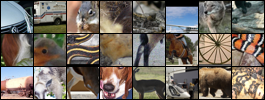
The input to the proposed training procedure is a set of unlabeled images, which come from roughly the same distribution as the images in which we later aim to compute the learned features. We randomly sample $N$ patches of size $32\times 32$ pixels from different images at varying positions and scales forming the initial training set $X=\{\mathbf{x}_{1},\ldots\mathbf{x}_{N}\}$. We are interested in patches containing objects or parts of objects, hence we sample only from regions containing considerable gradients. More precisely, we sample a patch with probability proportional to mean squared gradient magnitude within the patch. Exemplary patches sampled from the STL-10 unlabeled dataset are shown in Fig. 2.

We define a family of transformations $\{T_{\mathbf{\alpha}}|\,\mathbf{\alpha}\in\mathcal{A}\}$ parameterized by vectors $\mathbf{\alpha}\in\mathcal{A}$, where $\mathcal{A}$ is the set of all possible parameter vectors. Each transformation $T_{\mathbf{\alpha}}$ is a composition of elementary transformations. To learn features for the purpose of object classification, we used transformations from the following list:

• translation: vertical and horizontal translation by a distance within $0.2$ of the patch size;

• scaling: multiplication of the patch scale by a factor between $0.7$ and $1.4$;

• rotation: rotation of the image by an angle up to $20$ degrees;

• contrast 1: multiply the projection of each patch pixel onto the principal components of the set of all pixels by a factor between $0.5$ and $2$ (factors are independent for each principal component and the same for all pixels within a patch);

• contrast 2: raise saturation and value (S and V components of the HSV color representation) of all pixels to a power between $0.25$ and $4$ (same for all pixels within a patch), multiply these values by a factor between $0.7$ and $1.4$, add to them a value between $-0.1$ and $0.1$;

• color: add a value between $-0.1$ and $0.1$ to the hue (H component of the HSV color representation) of all pixels in the patch (the same value is used for all pixels within a patch).

The approach is flexible with regard to extending this list by other transformations in order to serve other applications of the learned features better. For instance, in Section 5 we show that descriptor matching benefits from adding a blur transformation.

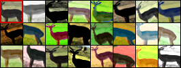
All numerical parameters of elementary transformations, when concatenated together, form a single parameter vector $\alpha$. For each initial patch $\mathbf{x}_{i}\in X$ we sample $K$ random parameter vectors $\{\mathbf{\alpha}_{i}^{1},\ldots,\mathbf{\alpha}_{i}^{K}\}$ and apply the corresponding transformations $\mathcal{T}_{i}=\{T_{\mathbf{\alpha}_{i}^{1}},\ldots,T_{\mathbf{\alpha}_{i}^{K}}\}$ to the patch $\mathbf{x}_{i}$. This yields the set of its transformed versions $S_{\mathbf{x}_{i}}=\mathcal{T}_{i}\mathbf{x}_{i}=\{T\mathbf{x}_{i}|\,T\in\mathcal{T}_{i}\}$. An example of such a set is shown in Fig. 2 . Afterwards we subtract the mean of each pixel over the whole resulting dataset. We do not apply any other preprocessing.

3 Learning Algorithm

Given the sets of transformed image patches, we declare each of these sets to be a class by assigning label $i$ to the class $S_{x_{i}}$. We train a CNN to discriminate between these surrogate classes. Formally, we minimize the following loss function:

$$L(X)=\sum\limits_{\mathbf{x}_{i}\in X}\sum\limits_{T\in\mathcal{T}_{i}}l(i,\,T\mathbf{x}_{i}),$$ (1)

where $l(i,\,T\mathbf{x}_{i})$ is the loss on the transformed sample $T\mathbf{x}_{i}$ with (surrogate) true label $i$. We use a CNN with a fully connected classification layer and a softmax output layer and we optimize the multinomial negative log likelihood of the network output, hence in our case

$$\begin{split}l(i,\,T\mathbf{x}_{i})&=M(\mathbf{e}_{i},f(T\mathbf{x}_{i})),\\ M(\mathbf{y},\mathbf{f})&=-\langle\mathbf{y},\,\log\mathbf{f}\rangle=-\sum\limits_{k}y_{k}\log f_{k},\end{split}$$ (2)

where $f(\cdot)$ denotes the function computing the values of the output layer of the CNN given the input data, and $\mathbf{e}_{i}$ is the $i$th standard basis vector. We note that in the limit of an infinite number of transformations per surrogate class, the objective function (1) takes the form

$$\widehat{L}(X)=\sum\limits_{\mathbf{x}_{i}\in X}\mathbb{E}_{\mathbf{\alpha}}[l(i,\,T_{\mathbf{\alpha}}\mathbf{x}_{i})],$$ (3)

which we shall analyze in the next section.

Intuitively, the classification problem described above serves to ensure that different input samples can be distinguished. At the same time, it enforces invariance to the specified transformations. In the following sections we provide a foundation for this intuition. We first present a formal analysis of the objective, separating it into a well defined classification problem and a regularizer that enforces invariance (resembling the analysis in [23]). We then discuss the derived properties of this classification problem and compare it to common practices for unsupervised feature learning.

3.1 Formal Analysis

We denote by $\mathbf{\alpha}\in\mathcal{A}$ the random vector of transformation parameters, by $g(\mathbf{x})$ the vector of activations of the second-to-last layer of the network when presented the input patch $\mathbf{x}$, by $\mathbf{W}$ the matrix of the weights of the last network layer, by $h(\mathbf{x})=\mathbf{W}g(\mathbf{x})$ the last layer activations before applying the softmax, and by $f(\mathbf{x})=\mathrm{softmax}\,(h(\mathbf{x}))$ the output of the network. By plugging in the definition of the softmax activation function

$$\mathrm{softmax}\,(\mathbf{z})=\exp(\mathbf{z})/\|\exp(\mathbf{z})\|_{1}$$ (4)

the objective function (3) with loss (2) takes the form

$$\sum\limits_{\mathbf{x}_{i}\in X}\mathbb{E}_{\mathbf{\alpha}}\bigl{[}-\langle\mathbf{e}_{i},\,h(T_{\mathbf{\alpha}}\mathbf{x}_{i})\rangle+\log\|\exp(h(T_{\mathbf{\alpha}}\mathbf{x}_{i}))\|_{1}\bigr{]}.$$ (5)

With $\widehat{\mathbf{g}_{i}}=\mathbb{E}_{\mathbf{\alpha}}\left[g(T_{\mathbf{\alpha}}\mathbf{x}_{i})\right]$ being the average feature representation of transformed versions of the image patch $\mathbf{x}_{i}$ we can rewrite Eq. (5) as

$$\begin{split}&\sum\limits_{\mathbf{x}_{i}\in X}\bigl{[}-\langle\mathbf{e}_{i},\,\mathbf{W}\widehat{\mathbf{g}_{i}}\rangle+\log\|\exp(\mathbf{W}\widehat{\mathbf{g}_{i}})\|_{1}\bigr{]}\\ +&\sum\limits_{\mathbf{x}_{i}\in X}\bigl{[}\mathbb{E}_{\mathbf{\alpha}}\left[\log\|\exp(h(T_{\mathbf{\alpha}}\mathbf{x}_{i}))\|_{1}\right]-\log\|\exp(\mathbf{W}\widehat{\mathbf{g}_{i}})\|_{1}\bigr{]}.\end{split}$$ (6)

The first sum is the objective function of a multinomial logistic regression problem with input-target pairs $(\widehat{\mathbf{g}_{i}},\,\mathbf{e}_{i})$. This objective falls back to the transformation-free instance classification problem $\overline{L}(X)=\sum_{\mathbf{x}_{i}\in X}l(i,\,\mathbf{x}_{i})$ if $g(\mathbf{x}_{i})=\mathbb{E}_{\mathbf{\alpha}}[g(T_{\mathbf{\alpha}}\mathbf{x})]$. In general, this equality does not hold and thus the first sum enforces correct classification of the average representation $\mathbb{E}_{\mathbf{\alpha}}[g(T_{\mathbf{\alpha}}\mathbf{x}_{i})]$ for a given input sample. For a truly invariant representation, however, the equality is achieved. Similarly, if we suppose that $T_{\mathbf{\alpha}}\mathbf{x}=\mathbf{x}$ for $\mathbf{\alpha}=0$, that for small values of $\mathbf{\alpha}$ the feature representation $g(T_{\mathbf{\alpha}}\mathbf{x}_{i})$ is approximately linear with respect to $\mathbf{\alpha}$ and that the random variable $\mathbf{\alpha}$ is centered, i.e. $\mathbb{E}_{\mathbf{\alpha}}\left[\mathbf{\alpha}\right]=0$, then $\widehat{\mathbf{g}_{i}}=\mathbb{E}_{\mathbf{\alpha}}\left[g(T_{\mathbf{\alpha}}\mathbf{x}_{i})\right]\approx\mathbb{E}_{\mathbf{\alpha}}\left[g(\mathbf{x}_{i})+\left.\nabla_{\mathbf{\alpha}}(g(T_{\mathbf{\alpha}}\mathbf{x}_{i}))\right|_{\mathbf{\alpha}=0}\,\mathbf{\alpha}\right]=g(\mathbf{x}_{i})$.

The second sum in Eq. (6) can be seen as a regularizer enforcing all $h(T_{\mathbf{\alpha}}\mathbf{x}_{i})$ to be close to their average value, i.e., the feature representation is sought to be approximately invariant to the transformations $T_{\mathbf{\alpha}}$. To show this we use the convexity of the function $\log\|\exp(\cdot)\|_{1}$ and Jensen’s inequality, which yields (proof in Appendix A):

$$\mathbb{E}_{\mathbf{\alpha}}\left[\log\|\exp(h(T_{\mathbf{\alpha}}\mathbf{x}_{i}))\|_{1}\right]-\log\|\exp(\mathbf{W}\widehat{\mathbf{g}_{i}})\|_{1}\geq 0.$$ (7)

If the feature representation is perfectly invariant, then $h(T_{\mathbf{\alpha}}\mathbf{x}_{i})=\mathbf{W}\widehat{\mathbf{g}_{i}}$ and inequality (7) turns to equality, meaning that the regularizer reaches its global minimum.

3.2 Conceptual Comparison to Previous Unsupervised Learning Methods

Suppose we want to unsupervisedly learn a feature representation useful for a recognition task, for example classification. The mapping from input images $\mathbf{x}$ to a feature representation $g(\mathbf{x})$ should then satisfy two requirements: (1) there must be at least one feature that is similar for images of the same category $\mathbf{y}$ (invariance); (2) there must be at least one feature that is sufficiently different for images of different categories (ability to discriminate).

Most unsupervised feature learning methods aim to learn such a representation by modeling the input distribution $p(\mathbf{x})$. This is based on the assumption that a good model of $p(\mathbf{x})$ contains information about the category distribution $p(\mathbf{y}|\mathbf{x})$. That is, if a representation is learned, from which a given sample can be reconstructed perfectly, then the representation is expected to also encode information about the category of the sample (ability to discriminate). Additionally, the learned representation should be invariant to variations in the samples that are irrelevant for the classification task, i.e., it should adhere to the manifold hypothesis (see e.g. [24] for a recent discussion). Invariance is classically achieved by regularization of the latent representation, e.g., by enforcing sparsity [12] or robustness to noise [13].

In contrast, the discriminative objective in Eq. (1) does not directly model the input distribution $p(\mathbf{x})$ but learns a representation that discriminates between input samples. The representation is not required to reconstruct the input, which is unnecessary in a recognition or matching task. This leaves more degrees of freedom to model the desired variability of a sample. As shown in our analysis (see Eq. (7)), we enforce invariance to transformations applied during surrogate data creation by requiring the representation $g(T_{\mathbf{\alpha}}\mathbf{x}_{i})$ of the transformed image patch to be predictive of the surrogate label assigned to the original image patch $\mathbf{x}_{i}$.

It should be noted that this approach assumes that the transformations $T_{\mathbf{\alpha}}$ do not change the identity of the image content. For example, if we use a color transformation we will force the network to be invariant to this change and cannot expect the extracted features to perform well in a task relying on color information (such as differentiating black panthers from pumas).

4 Experiments: Classification

To compare our discriminative approach to previous unsupervised feature learning methods, we report classification results on the STL-10 [25], CIFAR-10 [26], Caltech-101 [27] and Caltech-256 [28] datasets.

4.1 Experimental Setup

The datasets we tested on differ in the number of classes ($10$ for CIFAR and STL, $101$ for Caltech-101, $256$ for Caltech-256) and the number of samples per class. STL is especially well suited for unsupervised learning as it contains a large set of $100,\!000$ unlabeled samples. In all experiments, except for the dataset transfer experiment, we extracted surrogate training data from the unlabeled subset of STL-10. When testing on CIFAR-10, we resized the images from $32\times 32$ pixels to $64\times 64$ pixels to make the scale of depicted objects more similar to the other datasets. Caltech-101 images were resized to $150\times 150$ pixels and Caltech-256 images to $256\times 256$ pixels (Caltech-256 images have on average higher resolution than Caltech-101 images, so not downsampling them so much allows to preserve more fine details).

We worked with three network architectures. A smaller network was used to evaluate the influence of different components of the augmentation procedure on classification performance. It consists of two convolutional layers with $64$ filters each, followed by a fully connected layer with $128$ units. This last layer is succeeded by a softmax layer, which serves as the network output. This network will be referred to as 64c5-64c5-128f as explained in Appendix B.1.

To compare our method to the state-of-the-art we trained two bigger networks: a network that consists of three convolutional layers with $64$, $128$ and $256$ filters respectively followed by a fully connected layer with $512$ units (64c5-128c5-256c5-512f), and an even larger network, consisting of three convolutional layers with $92$, $256$ and $512$ filters respectively and a fully connected layer with $1024$ units (92c5-256c5-512c5-1024f).

In all these models all convolutional filters are connected to a $5\times 5$ region of their input. $2\times 2$ max-pooling was performed after the first and second convolutional layers. Dropout [29, 30] was applied to the fully connected layers. We trained the networks using an implementation based on Caffe [31]. Details on the training procedure and hyperparameter settings are provided in Appendix B.2.

TABLE I: Classification accuracies on several datasets (in percent). $*$ Average per-class accuracy  $78.0\%\pm 0.4\%$. $\dagger$ Average per-class accuracy  $85.0\%\pm 0.7\%$. $\ddagger$ Average per-class accuracy $85.8\%\pm 0.7\%$.

Algorithm	STL-10	CIFAR-10(400)	CIFAR-10	Caltech-101	Caltech-256(30)	#features
Convolutional K-means Network [32]	$60.1\pm 1$	$70.7\pm 0.7$	$82.0$	—	—	8000
Multi-way local pooling [33]	—	—	—	$77.3\pm 0.6$	$41.7$	$1024\times 64$
Slowness on videos [14]	$61.0$	—	—	$74.6$	—	556
Hierarchical Matching Pursuit (HMP) [34]	$64.5\pm 1$	—	—	—	—	1000
Multipath HMP [35]	—	—	—	$82.5\pm 0.5$	$50.7$	5000
View-Invariant K-means [16]	$63.7$	$72.6\pm 0.7$	$81.9$	—	—	6400
Exemplar-CNN (64c5-64c5-128f)	$67.1\pm 0.2$	$69.7\pm 0.3$	$76.5$	$79.8\pm 0.5^{*}$	$42.4\pm 0.3$	256
Exemplar-CNN (64c5-128c5-256c5-512f)	$72.8\pm 0.4$	$75.4\pm 0.2$	$82.2$	$86.1\pm 0.5^{\dagger}$	$51.2\pm 0.2$	960
Exemplar-CNN (92c5-256c5-512c5-1024f)	$\mathbf{74.2\pm 0.4}$	$\mathbf{76.6\pm 0.2}$	$\mathbf{84.3}$	$\mathbf{87.1\pm 0.7}^{\ddagger}$	$\mathbf{53.6\pm 0.2}$	1884
Supervised state of the art	$70.1$[36]	—	$92.0$ [37]	$91.44$ [38]	$70.6$ [2]	—

At test time we applied a network to arbitrarily sized images by convolutionally computing the responses of all the network layers except the top softmax (that is, we computed the responses of convolutional layers normally and then slided the fully connected layers on top of these). To the feature maps of each layer we applied the pooling method that is commonly used for the respective dataset:

1. 4-quadrant max-pooling, resulting in $4$ values per feature map, which is the standard procedure for STL-10 and CIFAR-10 [32, 14, 34, 16]

2. 3-layer spatial pyramid, i.e. max-pooling over the whole image as well as within 4 quadrants and within the cells of a $4\times 4$ grid, resulting in $1+4+16=21$ values per feature map, which is the standard for Caltech-101 and Caltech-256 [33, 14, 35]

Finally, we trained a one-vs-all linear support vector machine (SVM) on the pooled features.

On all datasets we used the standard training and test protocols. On STL-10 the SVM was trained on 10 pre-defined folds of the training data. We report the mean and standard deviation achieved on the fixed test set. For CIFAR-10 we report two results:

1. Training the SVM on the whole CIFAR-10 training set (called CIFAR-10)

2. The average over 10 random selections of 400 training samples per class (called CIFAR-10(400))

For Caltech-101 we follow the usual protocol of selecting 30 random samples per class for training and not more than 50 samples per class for testing. For Caltech-256 we randomly selected 30 samples per class for training and used the rest for testing. Both for Caltech-101 and Caltech-256 we repeated the testing procedure 10 times.

4.2 Classification Results

In Table 2 we compare Exemplar-CNN to several unsupervised feature learning methods, including the current state of the art on each dataset. We also list the state of the art for methods involving supervised feature learning (which is not directly comparable). Additionally we show the dimensionality of the feature vectors produced by each method before final pooling. The smallest network was trained on $8000$ surrogate classes containing $150$ samples each and the larger ones on $16000$ classes with $100$ samples each.

The features extracted from both larger networks outperform the best prior result on all datasets. This is despite the fact that the dimensionality of the feature vectors is smaller than that of most other approaches and that the networks are trained on the STL-10 unlabeled dataset (i.e. they are used in a transfer learning manner when applied to CIFAR-10 and Caltech). The increase in performance is especially pronounced when only few labeled samples are available for training the SVM, as is the case for all the datasets except full CIFAR-10. This is in agreement with previous evidence that with increasing feature vector dimensionality and number of labeled samples, training an SVM becomes less dependent on the quality of the features [32, 16]. Remarkably, on STL-10 we achieve an accuracy of $74.2\%$, which is a large improvement over all previously reported results.

4.3 Detailed Analysis

We performed additional experiments using the 64c5-64c5-128f network to study the effect of various design choices in Exemplar-CNN training and validate the invariance properties of the learned features.

TABLE II: Classification accuracies with clustering (in percent).

Algorithm	STL-10	CIFAR-10(400)	CIFAR-10	Caltech-101	Caltech-256(30)
64c5-64c5-128f	$69.5\pm 0.4$	$70.8\pm 0.2$	$76.8$	$79.5\pm 0.6$	$42.9\pm 0.3$
64c5-128c5-256c5-512f	$74.9\pm 0.4$	$75.7\pm 0.2$	$82.6$	$85.7\pm 0.6$	$51.4\pm 0.4$
92c5-256c5-512c5-1024f	$\mathbf{75.4\pm 0.3}$	$\mathbf{77.4\pm 0.2}$	$\mathbf{84.3}$	$\mathbf{87.2\pm 0.6}$	$\mathbf{53.7\pm 0.6}$

4.3.1 Number of Surrogate Classes

We varied the number $N$ of surrogate classes between $50$ and $32000$. As a sanity check, we also tried classification with random filters. The results are shown in Fig. 3.

Clearly, the classification accuracy increases with the number of surrogate classes until it reaches an optimum at about $8000$ surrogate classes after which it did not change or even decreased. This is to be expected: the larger the number of surrogate classes, the more likely it is to draw very similar or even identical samples, which are hard or impossible to discriminate. Few such cases are not detrimental to the classification performance, but as soon as such collisions dominate the set of surrogate labels, the discriminative loss is no longer reasonable and training the network to the surrogate task no longer succeeds. To check the validity of this explanation we also plot in Fig. 3 the validation error on the surrogate data after training the network. It rapidly grows as the number of surrogate classes increases, showing that the surrogate classification task gets harder with a growing number of classes. We observed that larger, more powerful networks reach their peak performance for more surrogate classes than smaller networks. However, the performance that can be achieved with larger networks saturates (not shown in the figure).

It can be seen as a limitation that sampling too many, too similar images for training can even decrease the performance of the learned features. It makes the number and selection of samples a relevant parameter of the training procedure. However, this drawback can be avoided for example by clustering.

To demonstrate this, given the STL-10 unlabeled dataset containing 100,000 images, we first train a 64c5-128c5-256c5-512f Exemplar-CNN on a subset of 16,000 image patches. We then use this Exemplar-CNN to extract descriptors of all images from the dataset and perform clustering similar to [39]. After discarding noisy and very similar clusters automatically (see Appendix B.3 for details), this leaves us with $6510$ clusters with approximately $10$ images in each of them. To the images in each cluster we then apply the same augmentation as in the original Exemplar-CNN. Each augmented cluster serves as a surrogate class for training. Table II shows the classification performance of the features learned by CNNs from this training data. Clustering increases the classification accuracy on all datasets, in particular on STL by up to $2.4$%, depending on the network. This shows that the small modification allows the approach to make use of large amounts of data. Potentially, using even more data or performing clustering and network training within a unified framework could further improve the quality of the learned features.

4.3.2 Number of Samples per Surrogate Class

Figure 3: Influence of the number of surrogate training classes. The validation error on the surrogate data is shown in red. Note the different y-axes for the two curves.

Figure 4: Classification performance on STL for different numbers of samples per class. Random filters can be seen as ’0 samples per class’.

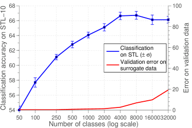
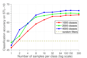
Fig. 4 shows the classification accuracy when the number $K$ of training samples per surrogate class varies between $1$ and $300$. The performance improves with more samples per surrogate class and saturates at around $100$ samples. This indicates that this amount is sufficient to approximate the formal objective from Eq. (3), hence further increasing the number of samples does not significantly change the optimization problem. On the other hand, if the number of samples is too small, there is not enough data to learn the desired invariance properties.

4.3.3 Types of Transformations

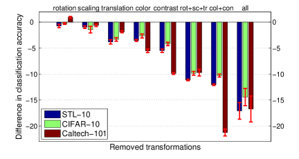
We varied the transformations used for creating the surrogate data to analyze their influence on the final classification performance. The set of ’seed’ patches was fixed. The result is shown in Fig. 5. The value ’$0$’ corresponds to applying random compositions of all elementary transformations: scaling, rotation, translation, color variation, and contrast variation. Different columns of the plot show the difference in classification accuracy as we discarded some types of elementary transformations.

Several tendencies can be observed. First, rotation and scaling have only a minor impact on the performance, while translations, color variations and contrast variations are significantly more important. Secondly, the results on STL-10 and CIFAR-10 consistently show that spatial invariance and color-contrast invariance are approximately of equal importance for the classification performance. This indicates that variations in color and contrast, though often neglected, may also improve performance in a supervised learning scenario. Thirdly, on Caltech-101 color and contrast transformations are much more important compared to spatial transformations than on the two other datasets. This is not surprising, since Caltech-101 images are often well aligned, and this dataset bias makes spatial invariance less useful.

We tried applying several other transformations (occlusion, affine transformation, additive Gaussian noise) in addition to the ones shown in Fig. 5, none of which seemed to improve the classification accuracy. For the matching task in Section 5, though, we found that using blur as an additional transformation improves the performance.

Figure 5: Influence of removing groups of transformations during generation of the surrogate training data. Baseline (’$0$’ value) is applying all transformations. Each group of three bars corresponds to removing some of the transformations.

Figure 6: Invariance properties of the feature representation learned by Exemplar-CNN. Top: transformations applied to an image patch (translation, rotation, contrast, saturation, color). Bottom: invariance of different feature representations. (a)-(c): Normalized Euclidean distance between feature vectors of the original and the translated image patches vs. the magnitude of the transformation, (d)-(f): classification performance on transformed image patches vs. the magnitude of the transformation for various magnitudes of transformations applied for creating the surrogate training data.

Figure 7: Filters learned by first layers of 64c5-64c5-128f networks when training on surrogate data from various dataset. Top – from STL-10, middle – CIFAR-10, bottom – Caltech-101.

4.3.4 Influence of the Dataset

We applied our feature learning algorithm to images sampled from three datasets – STL-10 unlabeled dataset, CIFAR-10 and Caltech-101 – and evaluated the performance of the learned feature representations on classification tasks on these datasets. We used the 64c5-64c5-128f network for this experiment.

We show the first layer filters learned from the three datasets in Fig. 7. Note how filters qualitatively differ depending on the dataset they were trained on.

Classification results are shown in Table III. The best classification results for each dataset are obtained when training on the patches extracted from the dataset itself. However, the difference is not drastic, indicating that the learned features generalize well to other datasets.

TABLE III: Dependence of classification performance (in %) on the training and testing datasets. Each column corresponds to different test data, each row to different training data (i.e. source of seed patches). We used the 64c5-64c5-128f network for this experiment.

	Testing
Training	STL-10	CIFAR-10(400)	Caltech-101
STL-10	$\mathbf{67.1\pm 0.3}$	$69.7\pm 0.3$	$79.8\pm 0.5$
CIFAR-10	$64.5\pm 0.4$	$\mathbf{70.3\pm 0.4}$	$77.8\pm 0.6$
Caltech-101	$66.2\pm 0.4$	$69.5\pm 0.2$	$\mathbf{80.0\pm 0.5}$

4.3.5 Influence of the Network Architecture on Classification Performance

We perform an additional experiment to evaluate the influence of the network architecture on classification performance. The results of this experiment are shown in Table IV. All networks were trained using a surrogate training set containing either $8000$ classes with $150$ samples each or $16000$ classes with $100$ samples each (for larger networks). We vary the number of layers, layer sizes and filter sizes. Classification accuracy generally improves with the network size indicating that our classification problem scales well to relatively large networks without overfitting.

TABLE IV: Classification accuracy depending on the network architecture. The name coding is as follows: NcF stands for a convolutional layer with $N$ filters of size $F\times F$ pixels, Nf stands for a fully connected layer with $N$ units. For example, 64c5-64c5-128f denotes a network with two convolutional layers containing 64 filters spanning $5\times 5$ pixels each, followed by a fully connected layer with $128$ units. We also show the number of surrogate classes used for training each network.

Architecture	#classes	STL-10	CIFAR-10(400)	CIFAR-10	Caltech-101
32c5-32c5-64f	8000	$63.8\pm 0.4$	$66.1\pm 0.4$	$71.3$	$78.2\pm 0.6$
64c5-64c5-128f	8000	$67.1\pm 0.3$	$69.7\pm 0.3$	$75.7$	$79.8\pm 0.5$
64c7-64c5-128f	8000	$66.3\pm 0.4$	$69.5\pm 0.3$	$75.0$	$79.4\pm 0.7$
64c5-64c5-64c5-128f	8000	$68.5\pm 0.3$	$70.9\pm 0.3$	$77.0$	$82.2\pm 0.7$
64c5-64c5-64c5-64c5-128f	8000	$64.7\pm 0.5$	$67.5\pm 0.3$	$75.2$	$75.7\pm 0.4$
128c5-64c5-128f	8000	$67.2\pm 0.4$	$69.9\pm 0.2$	$76.1$	$80.1\pm 0.5$
64c5-256c5-128f	8000	$69.2\pm 0.3$	$71.7\pm 0.3$	$77.9$	$81.6\pm 0.5$
64c5-64c5-512f	8000	$69.0\pm 0.4$	$71.7\pm 0.2$	$79.3$	$82.9\pm 0.4$
128c5-256c5-512f	8000	$71.2\pm 0.3$	$73.9\pm 0.3$	$81.5$	$84.3\pm 0.6$
128c5-256c5-512f	16000	$71.9\pm 0.3$	$74.3\pm 0.3$	$81.4$	$84.6\pm 0.6$
64c5-128c5-256c5-512f	16000	$72.8\pm 0.4$	$75.3\pm 0.3$	$82.0$	$85.5\pm 0.4$
92c5-256c5-512c5-1024f	16000	$73.9\pm 0.4$	$76.0\pm 0.2$	$83.6$	$86.9\pm 0.6$

4.3.6 Invariance Properties of the Learned Representation

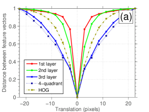
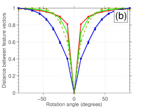
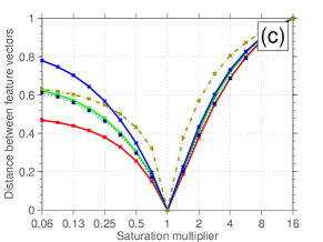
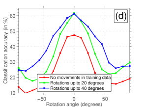
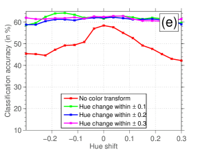
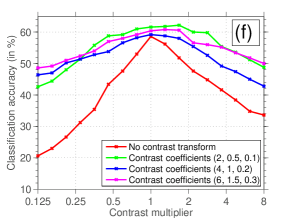
We analyzed to which extent the representation learned by the network is invariant to the transformations applied during training. We randomly sampled $500$ images from the STL-10 test set and applied a range of transformations (translation, rotation, contrast, color) to each image. To avoid empty regions beyond the image boundaries when applying spatial transformations, we cropped the central $64\times 64$ pixel sub-patch from each $96\times 96$ pixel image. We then applied two measures of invariance to these patches.

First, as an explicit measure of invariance, we calculated the normalized Euclidean distance between normalized feature vectors of the original image patch and the transformed one [14] (see Appendix C for details). The downside of this approach is that the distance between extracted features does not take into account how informative and discriminative they are. We therefore evaluated a second measure  – classification performance depending on the magnitude of the transformation applied to the classified patches  – which does not come with this problem. To compute the classification accuracy, we trained an SVM on the central $64\times 64$ pixel patches from one fold of the STL-10 training set and measured classification performance on all transformed versions of $500$ samples from the test set.

The results of both experiments are shown in Fig. 6. Overall the experiment empirically confirms that the Exemplar-CNN objective leads to learning invariant features. Features in the third layer and the final pooled feature representation compare favorably to a HOG baseline (Fig. 6 (a), (b)). This is consistent with the results we get in Section 5 for descriptor matching, where we compare the features to SIFT (which is similar to HOG).

Fig. 6(d)-(f) further show that stronger transformations in the surrogate training data lead to a more invariant classification with respect to these transformations. However, adding too much contrast variation may deteriorate classification performance (Fig. 6 (f)). One possible reason is that the contrast level can be a useful feature: for example, strong edges in an image are usually more important than weak ones.

5 Experiments: Descriptor Matching

In recognition tasks, such as image classification and object detection, the invariance requirements are largely defined by object class labels. Consequently, providing these class labels already when learning the features should be advantageous. This can be seen in the comparison to the supervised state-of-the-art in Table 2, where supervised feature learning performs better than the presented approach.

In contrast, matching of interest points in two images should be independent of object class labels. As a consequence, there is no apparent reason, why feature learning using class annotation should outperform unsupervised feature learning. One could even imagine that the class annotation is confusing and yields inferior features for matching.

5.1 Compared Features

We compare the features learned by supervised and unsupervised convolutional networks and SIFT [40] features. For a long time SIFT has been the preferred descriptor in matching tasks (see [41] for a comparison).

As supervised CNN we used the AlexNet model trained on ImageNet available at [31]. The architecture of the network follows Krizhevsky et al. [1] and contains 5 convolutional layers followed by 2 fully connected layers. In the experiments, we extract features from one of the 5 convolutional layers of the network. For large input patch sizes, the output dimensionality is high, especially for lower layers. For the descriptors to be more comparable to SIFT, we decided to max-pool the extracted feature map down to a fixed $4\times 4$ spatial size which corresponds to the spatial resolution of SIFT pooling. Even though the spatial size is the same, the number of features per cell is larger than for SIFT.

As unsupervised CNN we evaluated the matching performance of the 64c5-128c5-256c5-512f architecture, referred to as Exemplar-CNN-orig in the following. As the experiments show, neural networks cannot handle blur very well. Increasing image blur always leads to a matching performance drop. Hence we also trained another Exemplar-CNN to deal with this specific problem. First, we increased the filter size and introduced a stride of 2 in the first convolutional layer, resulting in the following architecture: 64c7s2-128c5-256c5-512f. This allows the network to identify edges in very blurry images more easily. Secondly, we used unlabeled images from Flickr for training, because these represent the general distribution of natural images better than STL. Thirdly, we applied blur of variable strength to the training data as an additional augmentation. We thus call this network Exemplar-CNN-blur. As with AlexNet, we max-pooled the feature maps produced by the Exemplar-CNNs to a $4\times 4$ spatial size.

5.2 Datasets

The common matching dataset by Mikolajczyk et al. [42] contains only $40$ image pairs. This dataset size limits the reliability of conclusions drawn from the results, especially as we compare various design choices, such as the depth of the network layer from which we draw the features. We set up an additional dataset that contains $384$ image pairs. It was generated by applying 6 different types of transformations with varying strengths to $16$ base images we obtained from Flickr. These images were not contained in the set we used to train the unsupervised CNN.

To each base image we applied the geometric transformations rotation, zoom, perspective, and nonlinear deformation. These cover rigid and affine transformations as well as more complex ones. Furthermore we applied changes to lighting and focus by adding blur. Each transformation was applied in various magnitudes such that its effect on the performance could be analyzed in depth. For each of the 16 base images we matched all the transformed versions of the image to the original one, which resulted in $384$ matching pairs.

The dataset from Mikolajczyk et al. [42] was not generated synthetically but contains real photos taken from different viewpoints or with different camera settings. While this reflects reality better than a synthetic dataset, it also comes with a drawback: the transformations are directly coupled with the respective images. Hence, attributing performance changes to either different image contents or to the applied transformations becomes impossible. In contrast, the new dataset enables us to evaluate the effect of each type of transformation independently of the image content.

Figure 8: Analysis of the matching performance depending on the patch size and the network layer at which features are computed.

5.3 Performance Measure

To evaluate the matching performance for a pair of images, we followed the procedure described in [41]. We first extracted elliptic regions of interest and corresponding image patches from both images using the maximally stable extremal regions (MSER) detector [43]. We chose this detector because it was shown to perform consistently well in [42] and it is widely used. For each detected region we extracted a patch according to the region scale and rotated it according to its dominant orientation. The descriptors of all extracted patches were greedily matched based on the Euclidean distance. This yielded a ranking of descriptor pairs. A pair was considered as a true positive if the ellipse of the descriptor in the target image and the ground truth ellipse in the target image had an intersection over union (IOU) of at least $0.5$. All other pairs were considered false positives. Assuming that a recall of 1 corresponds to the best achievable overall matching given the detections, we computed a precision-recall curve. The average precision, i.e., the area under this curve, was used as performance measure.

Figure 9: Scatter plots for different pairs of descriptors on the Flickr dataset (upper row) and the Mikolajczyk dataset (lower row). Each point in a scatter plot corresponds to one image pair, and its coordinates are the AP values obtained with the compared descriptors. AlexNet (supervised training) and the Exemplar-CNN yield features that outperform SIFT on most images of the Flickr dataset (a,b), but AlexNet is inferior to SIFT on the Mikolajczyk dataset. Features obtained with the unsupervised training procedure outperform the features from AlexNet on both datasets (c,f).

5.4 Patch size and network layer

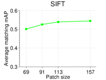
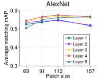
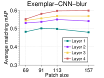
The MSER detector returns ellipses of varying sizes, depending on the scale of the detected region. To compute descriptors from these elliptic regions we normalized the image patches to a fixed size. It is not immediately clear which patch size is best: larger patches provide a higher resolution, but enlarging them too much may introduce interpolation artifacts and the effect of high-frequency noise may be emphasized. Therefore, we optimized the patch size on the Flickr dataset for each method.

When using convolutional neural networks for region description, aside from the patch size there is another fundamental choice – the network layer from which the features are extracted. Features from higher layers are more abstract.

Fig. 8 shows the average performance of each method when varying the patch size between $69$ and $157$. We chose the maximum patch size value such that most ellipses are smaller than that. We found that in case of SIFT, the performance monotonously grows and saturates at the maximum patch size. SIFT is based on normalized finite differences, and thus very robust to blurred edges caused by interpolation. In contrast, for the networks, especially for their lower layers, there is an optimal patch size, after which performance starts degrading. The lower network layers typically learn Gabor-like filters tuned to certain frequencies. Therefore, they suffer from over-smoothing caused by interpolation. Features from higher layers have access to larger receptive fields and, thus, can again benefit from larger patch sizes.

In the following experiments we used the optimal parameters given by Fig. 8: patch size $157$ for SIFT and $113$ for all other methods; layer $4$ for AlexNet and Exemplar-CNN-blur and layer $3$ for Exemplar-CNN-orig.

Figure 10: Mean average precision on the Flickr dataset for various transformations. Except for the blur transformation, all networks perform consistently better than SIFT. The network trained with blur transformations can keep up with SIFT even on blur.

Figure 11: Mean average precision on the Mikolajczyk dataset. The networks perform better on viewpoint transformations, while SIFT is more robust to strong blur and lighting transformations.

5.5 Results

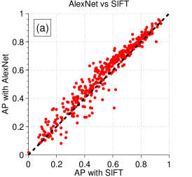
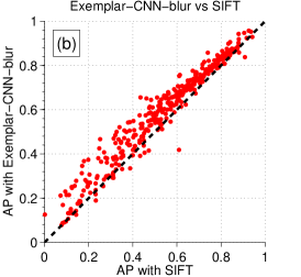
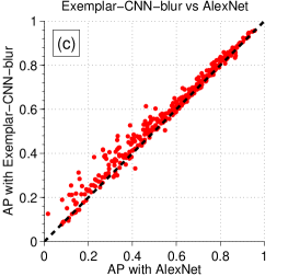
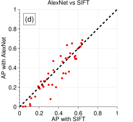
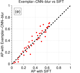
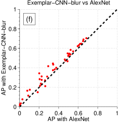
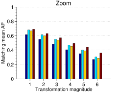
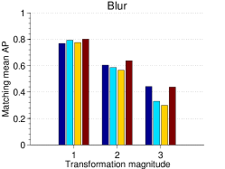
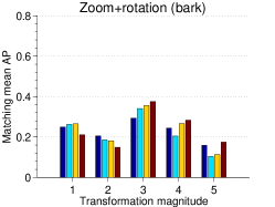
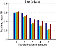
Fig. 9 shows scatter plots that compare the performance of pairs of methods in terms of average precision. Each dot corresponds to an image pair. Points above the diagonal indicate better performance of the first method, and for points below the diagonal the AP of the second method is higher. The scatter plots also give an intuition of the variance in the performance difference.

Fig. 9a,b show that the features from both AlexNet and the Exemplar-CNN outperform SIFT on the Flickr dataset. However, especially for features from AlexNet there are some image pairs, for which SIFT performs clearly better. On the Mikolayczyk dataset, SIFT even outperforms features from AlexNet. We will analyze this in more detail in the next paragraph. Fig. 9c,f compare AlexNet with the Exemplar-CNN-blur and show that the loss function based on surrogate classes is superior to the loss function based on object class labels. In contrast to object classification, class-specific features are not advantageous for descriptor matching. A loss function that focuses on the invariance properties required for descriptor matching yields better results.

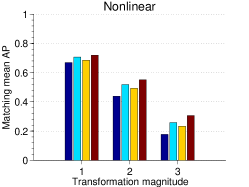
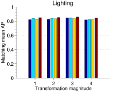
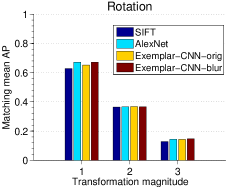
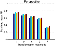
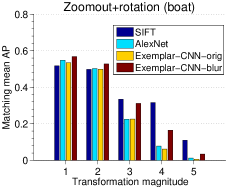
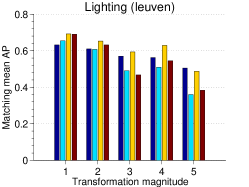
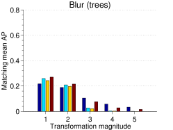
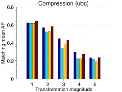
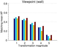
In Fig. 10 and 11 we analyze the reason for the clearly inferior performance of AlexNet on some image pairs. The figures show the mean average precision on the various transformations of the datasets using the optimized parameters. On the Flickr dataset AlexNet performs better than SIFT for all transformations except blur, where there is a big drop in performance. Also on the Mikolayczyk dataset, the blur and zoomout transformations are the main reason for SIFT performing better overall. Actually this effect is not surprising. At the lower layers, the networks mostly contain filters that are tuned to certain frequencies. Also the features at higher layers seem to expect a certain sharpness for certain image structures. Consequently, a blurred version of the same image activates very different features. In contrast, SIFT is very robust to image blur as it uses simple finite differences that indicate edges at all frequencies, and the edge strength is normalized out.

The Exemplar-CNN-blur is much less affected by blur since it has learned to be robust to it. To demonstrate the importance of adding blur to the transformations, we also included the Exemplar-CNN which was used for the classification task, i.e., without blur among the transformations. Like AlexNet, it has problems with matching blurred images to the original image.

Computation times per image are shown in Table V. SIFT computation is clearly faster than feature computation by neural networks, but the computation times of the neural networks are not prohibitively large, especially when extracting many descriptors per image using parallel hardware.

Method	SIFT	AlexNet	Ex-CNN-blur
CPU	$\,4.5\mathrm{ms}$	$\,28.2\mathrm{ms}$	$\,103.9\mathrm{ms}$
GPU	-	$\,0.7\mathrm{ms}$	$\,1.8\mathrm{ms}$

TABLE V: Feature computation times for a patch of 113 by 113 pixels.

6 Conclusions

We have proposed a discriminative objective for unsupervised feature learning by training a CNN without object class labels. The core idea is to generate a set of surrogate labels via data augmentation, where the applied transformations define the invariance properties that are to be learned by the network. The learned features yield a large improvement in classification accuracy compared to features obtained with previous unsupervised methods. These results strongly indicate that a discriminative objective is superior to objectives previously used for unsupervised feature learning. The unsupervised training procedure also lends itself to learn features for geometric matching tasks. A comparison to the long standing state-of-the-art descriptor for this task, SIFT, revealed a problem when matching neural network features in case of blur. We showed that by adding blur to the set of transformations applied during training, the features obtained with such a network are not much affected by this problem anymore and outperform SIFT on most image pairs. This simple inclusion of blur demonstrates the flexibility of the proposed unsupervised learning strategy. The strong relationship of the approach to data augmentation in supervised settings also emphasizes the value of data augmentation in general and suggests the use of more diverse transformations.

Appendix A Formal analysis

Proposition 1

The function

$$Z(\mathbf{x})=\log\|\exp(\mathbf{x})\|_{1},\;\mathbf{x}~{}\in~{}\mathbb{R}^{n}$$

is convex. Moreover, for any $\mathbf{x}\in\mathbb{R}^{n}$ the kernel of its Hessian matrix $\nabla^{2}Z(\mathbf{x})$ is given by $span\,(\mathbf{1})$

Proof:

Since

$$Z(\mathbf{x})=\log\|\exp(\mathbf{x})\|_{1}=\log\sum_{i=1}^{n}\exp(x_{i})$$ (8)

we need to prove the convexity of the log-sum-exp function. The Hessian $\nabla^{2}$ of this function is given as

$$\nabla^{2}Z(\mathbf{x})=\frac{1}{(\mathbf{1}^{T}\mathbf{u})^{2}}((\mathbf{1}^{T}\mathbf{u})\;diag\,(\mathbf{u})-\mathbf{u}\mathbf{u}^{T}),$$ (9)

with $\mathbf{u}=exp(\mathbf{x})$ and $\mathbf{1}\in\mathbb{R}^{n}$ being a vector of ones. To show the convexity we must prove that $\mathbf{z}^{T}\nabla^{2}Z(\mathbf{x})\mathbf{z}\geq 0$ for all $\mathbf{x},\mathbf{z}\in\mathbb{R}^{n}$. From (9) we get

$$\mathbf{z}^{T}\,\nabla^{2}Z(\mathbf{x})\,\mathbf{z}=\frac{1}{(\mathbf{1}^{T}\mathbf{u})^{2}}((\mathbf{1}^{T}\mathbf{u})\;\mathbf{z}^{T}diag\,(\mathbf{u})\,\mathbf{z}-\mathbf{z}^{T}\mathbf{u}\mathbf{u}^{T}\mathbf{z})\\ =\frac{(\sum_{k=1}^{n}u_{k}z_{k}^{2})(\sum_{k=1}^{n}u_{k})-(\sum_{k=1}^{n}u_{k}z_{k})^{2}}{(\sum_{k=1}^{n}u_{k})^{2}}\geq 0$$ (10)

since $(\sum_{k=1}^{n}u_{k})^{2}\geq 0$ and $(\sum_{k=1}^{n}z_{k}u_{k})^{2}\leq(\sum_{k=1}^{n}u_{k}z_{k}^{2})(\sum_{k=1}^{n}u_{k})$ due to the Cauchy-Schwarz inequality.

Inequality (10) only turns to equality if

$$\sqrt{u_{k}}z_{k}=c\sqrt{u_{k}},$$ (11)

where the constant $c$ does not depend on $k$. This immediately gives $\mathbf{z}=c\mathbf{1}$, which proves the second statement of the proposition. ∎

Proposition 2

Let $\mathbf{\alpha}\in\mathcal{A}$ be a random vector with values in a bounded set $\mathcal{A}\subset\mathbb{R}^{k}$. Let $\mathbf{x}(\cdot)\colon\,\mathcal{A}\to\mathbb{R}^{n}$ be a continuous function. Then inequality (7)

$$\mathbb{E}_{\mathbf{\alpha}}\left[\log\|\exp(\mathbf{x}(\mathbf{\alpha}))\|_{1}\right]-\log\|\exp(\mathbb{E}_{\mathbf{\alpha}}[\mathbf{x}(\mathbf{\alpha})])\|_{1}\geq 0$$

holds and only turns to equality if for all $\mathbf{\alpha}_{1},\mathbf{\alpha}_{2}\in\mathcal{A}$: $(\mathbf{x}(\mathbf{\alpha}_{1})-\mathbf{x}(\mathbf{\alpha}_{2}))\in span\,(\mathbf{1})$ .

Proof:

Inequality (7) immediately follows from convexity of the function $\log\|\exp(\cdot)\|_{1}$ and Jensen’s inequality.

Jensen’s inequality only turns to equality if the function it is applied to is affine-linear on the convex hull of the integration region. In particular this implies

$$(\mathbf{x}(\mathbf{\alpha}_{1})-\mathbf{x}(\mathbf{\alpha}_{2}))^{T}\;\nabla^{2}Z(\mathbf{x}(\mathbf{\alpha}_{1}))\;(\mathbf{x}(\mathbf{\alpha}_{1})-\mathbf{x}(\mathbf{\alpha}_{2}))=0$$ (12)

for all $\mathbf{\alpha}_{1},\mathbf{\alpha}_{2}\in\mathcal{A}$. The second statement of Proposition 1 thus immediately gives $\mathbf{x}(\mathbf{\alpha}_{1})-\mathbf{x}(\mathbf{\alpha}_{2})=c\mathbf{1}$, Q.E.D.

∎

Appendix B Method details

We describe here in detail the network architectures we evaluated and explain the network training procedure. We also provide details of the clustering process we used to improve Exemplar-CNN.

B.1 Network Architecture

We tested various network architectures in combination with our training procedure. They are coded as follows: NcF stands for a convolutional layer with $N$ filters of size $F\times F$ pixels, Nf stands for a fully connected layer with $N$ units. For example, 64c5-64c5-128f denotes a network with two convolutional layers containing 64 filters spanning $5\times 5$ pixels each followed by a fully connected layer with $128$ units. The last specified layer is always succeeded by a softmax layer, which serves as the network output. We applied $2\times 2$ max-pooling to the outputs of the first and second convolutional layers.

As stated in the paper we used a 64c5-64c5-128f architecture in our experiments to evaluate the influence of different components of the augmentation procedure (we refer to this architecture as the ’small’ network). A large network, coded as 64c5-128c5-256c5-512f, was then used to achieve better classification performance.

All considered networks contained rectified linear units in each layer but the softmax layer. Dropout was applied to the fully connected layer.

B.2 Training the Networks

We adopted the common practice of training the network with stochastic gradient descent with a fixed momentum of $0.9$. We started with a learning rate of $0.01$ and gradually decreased the learning rate during training. That is, we trained until there was no improvement in validation error, then decreased the learning rate by a factor of $3$, and repeated this procedure until convergence. Training times on a Titan GPU were roughly $1.5$ days for the 64c5-64c5-128f network, $4$ days for the 64c5-128c5-256c5-512f network and $9$ days for the 92c5-256c5-512c5-1024f network.

B.3 Clustering

To judge about similarity of the clusters we use the following simple heuristics. The method of [39] gives us a set of linear SVMs. We apply these SVMs to the whole STL-10 unlabeled dataset and select $N_{percluster}=10$ top firing images per SVM, which gives us a set of initial clusters. We then compute the overlap (number of common images) of each pair of these clusters. We set two thresholds $T_{merge}=3$ and $T_{discard}=1$ and perform a greedy procedure: starting from the most overlapping pair of clusters, we merge the clusters if their overlap exceeds $T_{merge}$ and discard one of the clusters if the overlap is between $T_{discard}$ and $T_{merge}$.

Appendix C Details of computing the measure of invariance

We now explain in detail and motivate the computation of the normalized Euclidean distance used as a measure of invariance in the paper.

First we compute feature vectors of all image patches and their transformed versions. Then we normalize each feature vector to unit Euclidean norm and compute the Euclidean distances between each original patch and all of its transformed versions. For each transformation and magnitude we average these distances over all patches. Finally, we divide the resulting curves by their maximal values (typically it is the value for the maximum magnitude of the transformation).

The normalizations are performed to compensate for possibly different scales of different features. Normalizing feature vectors to unit length ensures that the values are in the same range for different features. The final normalization of the curves by the maximal value allows to compensate for different variation of different features: as an extreme, a constant feature would be considered perfectly invariant without this normalization, which is certainly not desirable.

The resulting curves show how quickly the feature representation changes when an image is transformed more and more. A representation for which the curve steeply goes up and then remains constant cannot be considered invariant to the transformation: the feature vector of the transformed patch becomes completely uncorrelated with the original feature vector even for small magnitudes of the transformation. On the other hand, if the curve grows gradually, this indicates that the feature representation changes slowly when the transformation is applied, meaning invariance or, rather, covariance of the representation.

References

- [1] A. Krizhevsky, I. Sutskever, and G. E. Hinton, “ImageNet classification with deep convolutional neural networks,” in NIPS, 2012, pp. 1106–1114.
- [2] M. D. Zeiler and R. Fergus, “Visualizing and understanding convolutional networks,” in ECCV, 2014.
- [3] J. Donahue, Y. Jia, O. Vinyals, J. Hoffman, N. Zhang, E. Tzeng, and T. Darrell, “DeCAF: A deep convolutional activation feature for generic visual recognition,” in ICML, 2014.
- [4] A. S. Razavian, H. Azizpour, J. Sullivan, and S. Carlsson, “CNN features off-the-shelf: An astounding baseline for recognition,” in CVPR Workshops 2014, 2014, pp. 512–519.
- [5] R. Girshick, J. Donahue, T. Darrell, and J. Malik, “Rich feature hierarchies for accurate object detection and semantic segmentation,” in CVPR, 2014.
- [6] P. Sermanet, D. Eigen, X. Zhang, M. Mathieu, R. Fergus, and Y. LeCun, “OverFeat: Integrated recognition, localization and detection using convolutional networks.” in ICLR, 2014.
- [7] B. Hariharan, P. Arbeláez, R. Girshick, and J. Malik, “Hypercolumns for object segmentation and fine-grained localization,” CVPR, 2015.
- [8] J. Long, E. Shelhamer, and T. Darrell, “Fully convolutional networks for semantic segmentation,” in CVPR, 2015.
- [9] J. Deng, W. Dong, R. Socher, L.-J. Li, K. Li, and L. Fei-Fei, “ImageNet: A Large-Scale Hierarchical Image Database,” in CVPR, 2009.
- [10] M. Everingham, L. Gool, C. K. Williams, J. Winn, and A. Zisserman, “The Pascal Visual Object Classes (VOC) Challenge,” IJCV, vol. 88, no. 2, pp. 303–338, 2010.
- [11] Y. LeCun, B. Boser, J. S. Denker, D. Henderson, R. E. Howard, W. Hubbard, and L. D. Jackel, “Backpropagation applied to handwritten zip code recognition,” Neural Computation, vol. 1, no. 4, pp. 541–551, 1989.
- [12] K. Kavukcuoglu, P. Sermanet, Y. Boureau, K. Gregor, M. Mathieu, and Y. LeCun, “Learning convolutional feature hierachies for visual recognition,” in NIPS, 2010.
- [13] P. Vincent, H. Larochelle, Y. Bengio, and P.-A. Manzagol, “Extracting and composing robust features with denoising autoencoders,” in ICML, 2008, pp. 1096–1103.
- [14] W. Y. Zou, A. Y. Ng, S. Zhu, and K. Yu, “Deep learning of invariant features via simulated fixations in video,” in NIPS, 2012, pp. 3212–3220.
- [15] K. Sohn and H. Lee, “Learning invariant representations with local transformations,” in ICML, 2012.
- [16] K. Y. Hui, “Direct modeling of complex invariances for visual object features,” in ICML, 2013.
- [17] P. Simard, B. Victorri, Y. LeCun, and J. S. Denker, “Tangent Prop - A formalism for specifying selected invariances in an adaptive network,” in NIPS, 1992.
- [18] H. Drucker and Y. LeCun, “Improving generalization performance using double backpropagation,” IEEE Transactions on Neural Networks, vol. 3, no. 6, pp. 991–997, 1992.
- [19] M.-R. Amini and P. Gallinari, “Semi supervised logistic regression,” in ECAI, 2002, pp. 390–394.
- [20] Y. Grandvalet and Y. Bengio, “Entropy regularization,” in Semi-Supervised Learning. MIT Press, 2006, pp. 151–168.
- [21] A. Ahmed, K. Yu, W. Xu, Y. Gong, and E. Xing, “Training hierarchical feed-forward visual recognition models using transfer learning from pseudo-tasks.” in ECCV (3), 2008, pp. 69–82.
- [22] R. Collobert, J. Weston, L. Bottou, M. Karlen, K. Kavukcuoglu, and P. Kuksa, “Natural language processing (almost) from scratch,” Journal of Machine Learning Research, vol. 12, pp. 2493–2537, 2011.
- [23] S. Wager, S. Wang, and P. Liang, “Dropout training as adaptive regularization,” in NIPS, 2013.
- [24] S. Rifai, Y. N. Dauphin, P. Vincent, Y. Bengio, and X. Muller, “The manifold tangent classifier,” in NIPS, 2011.
- [25] A. Coates, H. Lee, and A. Y. Ng, “An analysis of single-layer networks in unsupervised feature learning,” AISTATS, 2011.
- [26] A. Krizhevsky and G. Hinton, “Learning multiple layers of features from tiny images,” Master’s thesis, Department of Computer Science, University of Toronto, 2009.
- [27] L. Fei-Fei, R. Fergus, and P. Perona, “Learning generative visual models from few training examples: An incremental bayesian approach tested on 101 object categories,” in CVPR WGMBV, 2004.
- [28] G. Griffin, A. Holub, and P. Perona, “Caltech-256 object category dataset,” California Institute of Technology, Tech. Rep. 7694, 2007.
- [29] G. E. Hinton, N. Srivastava, A. Krizhevsky, I. Sutskever, and R. R. Salakhutdinov, “Improving neural networks by preventing co-adaptation of feature detectors,” 2012, pre-print, arxiv:cs/1207.0580v3.
- [30] N. Srivastava, G. Hinton, A. Krizhevsky, I. Sutskever, and R. Salakhutdinov, “Dropout: A simple way to prevent neural networks from overfitting,” Journal of Machine Learning Research, vol. 15, pp. 1929–1958, 2014.
- [31] Y. Jia, E. Shelhamer, J. Donahue, S. Karayev, J. Long, R. Girshick, S. Guadarrama, and T. Darrell, “Caffe: Convolutional architecture for fast feature embedding,” arXiv preprint arXiv:1408.5093, 2014.
- [32] A. Coates and A. Y. Ng, “Selecting receptive fields in deep networks,” in NIPS, 2011, pp. 2528–2536.
- [33] Y. Boureau, N. Le Roux, F. Bach, J. Ponce, and Y. LeCun, “Ask the locals: multi-way local pooling for image recognition,” in ICCV’11. IEEE, 2011.
- [34] L. Bo, X. Ren, and D. Fox, “Unsupervised feature learning for RGB-D based object recognition,” in ISER, June 2012.
- [35] ——, “Multipath sparse coding using hierarchical matching pursuit,” in CVPR, 2013, pp. 660–667.
- [36] K. Swersky, J. Snoek, and R. P. Adams, “Multi-task bayesian optimization,” in NIPS, 2013.
- [37] C.-Y. Lee, S. Xie, P. Gallagher, Z. Zhang, and Z. Tu, “Deeply supervised nets,” in Deep Learning and Representation Learning Workshop, NIPS, 2014.
- [38] K. He, X. Zhang, S. Ren, and J. Sun, “Spatial pyramid pooling in deep convolutional networks for visual recognition,” in ECCV, 2014.
- [39] S. Singh, A. Gupta, and A. A. Efros, “Unsupervised discovery of mid-level discriminative patches,” in ECCV, 2012.
- [40] D. G. Lowe, “Distinctive image features from scale-invariant keypoints,” IJCV, vol. 60, no. 2, pp. 91–110, Nov. 2004.
- [41] K. Mikolajczyk and C. Schmid, “A performance evaluation of local descriptors,” IEEE Trans. Pattern Anal. Mach. Intell., vol. 27, no. 10, pp. 1615–1630, 2005.
- [42] K. Mikolajczyk, T. Tuytelaars, C. Schmid, A. Zisserman, J. Matas, F. Schaffalitzky, T. Kadir, and L. J. V. Gool, “A comparison of affine region detectors,” IJCV, vol. 65, no. 1-2, pp. 43–72, 2005.
- [43] J. Matas, O. Chum, M. Urban, and T. Pajdla, “Robust wide baseline stereo from maximally stable extremal regions,” in Proc. BMVC, 2002, pp. 36.1–36.10, doi:10.5244/C.16.36.