Model of lateral diffusion in ultrathin layered films

Abstract

We consider the diffusion of markers in a layered medium, with the lateral diffusion coefficient being the function of hight. We show that the probability density of the lateral displacements follows one-dimensional Batchelor’s equation with time-dependent diffusion coefficient governed by the particles’ redistribution in height. For the film of a finite thickness the resulting mean squared displacement exhibits superdiffusion at short times and crosses over to normal diffusion at long times. The approach is used for description of experimental results on inhomogeneous molecular diffusion in thin liquid films deposited on solid surfaces.

Highlights:

• We show that vertical layering of liquid leads to superdiffusion behavior of walking markers

• Finite film thickness cause the asymptotical transition from superdiffusion to normal diffusion

• Conditional independence of orthogonal walks for 2D Fokker-Plank equation gives 1D Batchelor’s

1 Introduction

Recent experimental research of diffusion and trapping of single particles of $\mu$- and nm-scales in confined liquid films [1, 2, 3, 4, 5, 6] show that this process presents non-trivial behavior considerably different from a usual Brownian diffusion in a bulk due to strong interaction of ultrathin fluid matrix with a base solid interface. The detailed single-molecule tracking detects the dependence of diffusivity on a distance of layer from the interface. It should be noted that a majority of evaluated experiments deals with the study of hydrodynamic interaction of colloid particles with a rigid wall that leads to change of both vertical and horizontal diffusivities [7]. However, the very important parameter of such a system is a particle’s size [1]. It has been found [8, 4, 5, 6] that the experiments with micrometer-scale spherical particles diffusing in a uniform fluid close to the wall quite satisfactory admit the two-dimensional depth-dependent anisotropic diffusion approach of [7].

At the same time, it was mentioned [3] that particle size change from $\mu$-m to nm scales leads to large deviations from hydrodynamic theory. Particularly, in the experimental work [3] it was demonstrated that observed vertical diffusion coefficient is smaller. The discussion in [3] attributes this fact to the prevalence of intermolecular forces over hydrodynamical ones for such scales. From this point of view, very important experimental study was evaluated in the work [2], where extremely small (molecular-size) markers were traced. It has bean detected there that the lateral diffusion is anomalous (superdiffusion) for short times and crosses over to normal diffusion for long times. This phenomenon was discussed in a connection with the fact that fluids close to wetted interfaces are know to form a layered structure.

The motion of molecules in such layered structures can be described within the following random walk picture. The layers close to the interface are practically frozen and the lateral motion in these layers is slow. However, particles can diffuse (jump) vertically to layers, where the random walks are faster. Thus, the transient diffusive behavior is based on a coexistence of these vertical and lateral jumps. Note that the process of molecular diffusion in a wetting layer differs from the one of macroscopic particles near the wall which can be described using the hydrodynamical picture [7], vide infra.

In what follows we adopt a coarse-grained description and consider the continuous model of layered diffusion: The particle performs diffusive motion in $y$-direction. The properties of this motion are independent on the particle’s lateral position due to translational symmetry of the fluid layer in this direction, while the properties of diffusion in $x$-direction depend on the particle’s distance from the surface (i.e. on its $y$-coordinate). Our model thus corresponds to a one of the layered system.

The models of layered diffusion correspond to cases when the properties of motion in one ($y$) direction (normal to layers) do not depend on the coordinate $x$, while the motion within layers (in $x$-direction) depends on $y$. The properties of motions in $x$ and $y$-directions differ, defining different models of layered diffusion: Thus the combination of continuous drift in $y$ with random velocity model in $x$ defines Taylor’s model of “Diffusion by continuous motions” [9], the combination of diffusion in $y$ with the same random velocity model in $x$ defines a superdiffusive Matheron—De Marsily model [10], and combination of diffusion in $y$ with transport with deterministic mean velocity proportional to $y$ defines the model of diffusion in a shear flow introduced by Novikov [11]. More general $y$-dependences of $x$-velocity define a class of models in [12].

The model of a layered system is not limited to hydrodynamical situations. Thus, a similar model was recently used for modeling of superdiffusion in a small world network [13]. Namely, the set of slow walks along a regular background lattice and fast jumps along “short links” was replaced by the set of simple diffusion equations with the hierarchy diffusion coefficients depending on the distance between background nodes.

2 The model

A simple model described here adds an interesting example to the theory of diffusion in layered systems and gives rise to an effective equation of the Batchelor’s type for lateral diffusion. Due to symmetry in the directions parallel to the surface, it is enough to consider one lateral coordinate, which is denoted $x$ in what follows. For this reason we consider 2D picture at first. Then we discuss the generalization on 3D case, which is quite straightforward. Our model corresponds thus to a particle performing diffusion in $x$ and $y$-directions, where the properties of the vertical diffusion (in $y$-direction) do not depend on $x$. On a coarse-grained level (the steps of a random walk are not resolved) this model is described by a pair of Langevin equations

$$\dot{y} = \sqrt{2D_{y}}\xi_{y}(t)$$ (1)

$$\dot{x} = \sqrt{2D_{x}(y)}\xi_{x}(t)$$ (2)

with $D_{y}$ and $D_{x}(y)$ being the diffusion coefficients in $y$- and in $x$-directions, and $\xi_{y}(t)$, $\xi_{x}(t)$ being Gaussian white noises with zero mean and correlation property given by $\langle\xi_{\alpha}(t)\xi_{\beta}(t^{\prime})\rangle=\delta_{\alpha\beta}\delta(t-t^{\prime})$. Note that according to Eqs. (1) and (2) the motion in $y$ is independent on the motion in $x$-direction, while the motion in $x$ does depend on the actial $y$-coordinate through $D_{x}(y)$ and thus depends on the prehistory of $y$-motion. The random variables $x$ and $y$ are not independent.

The evolution of two-dimensional joint probability density $p(x,y,t)$ for marker’s position is then described by the Fokker-Planck equation corresponding to the equation of anisotropic diffusion:

$$\frac{\partial p}{\partial t}=D_{x}(y)\frac{\partial^{2}p}{\partial x^{2}}+D_{y}\frac{\partial^{2}p}{\partial y^{2}}.$$ (3)

The Dirac delta function $p(x,y,0)=\delta(x,y+0)$ is used as an initial condition. We are interested only in the time dependence of marginal distribution of $x$, which is experimentally accessible [2]. We note that although the situation with molecular tracer discussed here is different from the case of motion of a massive particle in a quiescent fluid, as discussed e.g. in [14], since a molecular motion is never underdamped. However, the final equation is exactly of the form obtained in this work, due to the fact that it is the only form corresponding to thermodynamical equilibrium (in the absence of external forces) in a stationary state.

Although Eq.(3) itself does not have to possess a solution which factorizes into a product of functions which depend only on one of the two co-ordinates, the solution of our physical problem given by Eqs.(1), (2) has to factorize: $p(x,y,t)=p(x,t)p(y,t)$, although $x$ and $y$ are not independent. The physical reason for this is as follows.

First let us remark, that while the two arguments $x$ and $y$ of $p(x,y,t)$ are the values of the corresponding random variables $x$ and $y$, its third argument, time, is not a random variable but essentially an additional condition: $p(x,y,t)=p(x,y|t)$ is a conditional joint probability of $x$ and $y$ provided their measurement took place at time $t$. Note now that according to Eq.(1) the motion in $y$ direction is independent on $x$, and moreover the initial condition for this motion in $y$ does not depend on $x$. Therefore the conditional probability of $y$ given $x$ is essentially a non-conditional one: $p(y|x,t)=p(y|t)$. According to Bayes theorem $p(x,y|t)=p(y|x,t)p(x|t)=p_{y}(y|t)p_{x}(x|t)$: the $x$ and $y$-displacements are conditionally independent [15]. Rewriting it in our initial notation we get

$$p(x,y,t)=p_{x}(x,t)p_{y}(y,t).$$ (4)

Independently on whether this discussion is convincing or not, one can always prove that the final solutions obtained by the separation ansatz are indeed the solutions of Eq.(3), i.e. that the product of Eq.(14) and Eq.(17) indeed solves Eq.(3) in an unbounded system with $D_{x}(y)=ky$, and that the product of Eq.(18) and of a symmetric Gaussian in $x$ with the dispersion given by Eq.(20) solves it for a layer of a finite thickness, as they indeed do.

Integrating both parts of Eq.(3) with respect to $x$ we obtain the equation for $p_{y}(y,t)$:

$$\frac{\partial p_{y}}{\partial t}=D_{y}\frac{\partial^{2}p_{y}}{\partial y^{2}}.$$ (5)

Inserting Eq.(4) into Eq.(3) and integrating over $y$ we obtain

$$\frac{\partial p_{x}}{\partial t}=\left[\int_{0}^{H}D(y)p_{y}(y,t)dy\right]\frac{\partial^{2}p_{x}}{\partial x^{2}},$$ (6)

with $H$ being the film’s thickness, i.e. the one-dimensional Batchelor’s equation [16]

$$\frac{\partial p_{x}}{\partial t}=D(t)\frac{\partial^{2}p_{x}}{\partial x^{2}},$$ (7)

with time-dependent diffusion coefficient

$$D(t)=\int_{0}^{H}D_{x}(y)p_{y}(y,t)dy.$$ (8)

Note that this Batchelor’s equation arises here not as the mean-field type approximation, but as an exact equation for the corresponding marginal probability density. Introducing a new variable $\tau=\int_{0}^{t}D(t)dt$ allows to reduce Eq. (7) to the simple diffusion equation

$$\frac{\partial p_{x}}{\partial\tau}=\frac{\partial^{2}p_{x}}{\partial x^{2}}.$$ (9)

Note that the change of variables from $t$ to $\tau$ is always possible within the model since the effective diffusion coefficient $D(t)$ given by Eq.(8) is always non-negative and therefore its integral over time is a monotonically growing (and therefore invertible) function. From this it follows that the corresponding probability density is Gaussian with a mean square displacement (MSD) $<x^{2}>=2\tau$.

In a 3D system uniform in $(x,z)$ coordinates with $D_{z}(y)=D_{x}(y)$ still depending on the vertical $y$ position, the system of Eqs. (1)–(2) is supplemented by

$$\dot{z}=\sqrt{2D_{x}(y)}\xi_{z}(t).$$ (10)

Thus, from the Eqs. (1)–(2), (10) and the symmetry in the directions parallel to the surface, it follows that the three-dimensional joint probability density $p(x,y,z,t)$ satisfies the equation:

$$\frac{\partial p}{\partial t}=D_{x}(y)\left[\frac{\partial^{2}p}{\partial x^{2}}+\frac{\partial^{2}p}{\partial z^{2}}\right]+D_{y}\frac{\partial^{2}p}{\partial y^{2}}.$$ (11)

As before, all displacements are conditionally independent and the three-dimensional joint probability density will be factorized as

$$p(x,y,z,t)=p_{x}(x,t)p_{y}(y,t)p_{z}(z,t).$$ (12)

The equation for $p_{z}(z,t)$ has exactly the form of the Eq. (9).

Finally, since the motions in both lateral directions are independent, the resulting MSD is

$$<r^{2}>=<x^{2}>+<z^{2}>=2<x^{2}>=4\tau.$$ (13)

In other words, it is simply two times larger then in 2D case, and the definition of $\tau$ follows from the Eq. (8) as above.

3 Solutions

3.1 Superdiffusion in a thick film

At first, we consider an idealized situation: the half-plane corresponding to the film of infinite thickness $H=\infty$. In this case the solution of Eq. (5) is the Gaussian

$$p_{y}(y,t)=\frac{1}{\sqrt{D_{y}\pi t}}\exp\left(-\frac{y^{2}}{4D_{y}t}\right).$$ (14)

Thereafter, one needs to determine the vertical dependence of the horizontal component of the diffusion coefficient. As it will be shown below, the experimental data are well-fitted by a linear dependence $D_{x}(y)=ky$. Under this condition, the substation (14) into (8) gives

$$D(t)=2k\sqrt{D_{y}t/\pi}.$$ (15)

Therefore, the averaged lateral mean-square displacement corresponds to the superdiffusion:

$$\left<x^{2}\right>=\frac{8k}{3}\sqrt{\frac{D_{y}}{\pi}}t^{\frac{3}{2}},$$ (16)

and the corresponding distribution of lateral positions is given by a Gaussian

$$p_{x}(x,t)=\frac{\exp\left(-\frac{x^{2}}{\sqrt{(4/9\pi)k^{2}D_{y}^{3}t^{3}}}\right)}{\sqrt[4]{(64/9)\pi k^{2}D_{y}^{3}t^{3}}}.$$ (17)

As it was discussed above, in 3D case additional multiplier $p_{z}(z,t)$ in the Eq. (12) will have exactly the same form as (17) with replacing $x\to z$, and MSD $<r^{2}>$ is given by twice the expression (16).

3.2 Film of finite thickness

Now let us consider the realistic situation, when the thickness $H$ is finite. In such a case the equation (5) with impenetrable boundaries has a standard solution in the form of the eigenfunction expansion:

$$p_{y}(y,t)=\frac{1}{H}+\frac{2}{H}\sum_{n=1}^{\infty}e^{-\frac{D_{y}\pi^{2}n^{2}}{H^{2}}t}\cos\left(\frac{\pi n}{H}y\right).$$ (18)

Under the same condition $D_{x}(y)=ky$, the time dependence of the averaged coefficient of lateral diffusion is represented by the series

$$D(t)=\frac{kH}{2}\left(1-\frac{8}{\pi^{2}}\sum_{m=0}^{\infty}\frac{e^{-\frac{D_{y}\pi^{2}(2m+1)^{2}}{H^{2}}t}}{(2m+1)^{2}}\right).$$ (19)

From Eq. (19) it follows that the effective diffusion coefficient is initially equal to zero due to sticking of a marker to the solid substrate, monotonically grows with time and then saturates. Its final value $D(\infty)=kH/2$ is achieved when the markers redistribute homogeneously over the whole liquid layer.

Integrating Eq. (19) over time we get the desired expression for a mean-square-displacement:

$$<x^{2}>=kH\left(t+\frac{8H^{2}}{D_{y}\pi^{4}}\sum_{m=0}^{\infty}\frac{e^{-\frac{D_{y}\pi^{2}(2m+1)^{2}}{H^{2}}t}-1}{(2m+1)^{4}}\right).$$ (20)

Analyzing Eq. (20), one can see that non-linear growth at a small time changes to the asymptotic linear one corresponding to a normal diffusion:

$$<x^{2}>_{\infty}=-\frac{kH^{3}}{12D_{y}}+kHt.$$ (21)

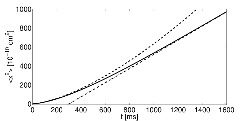
Fig. 1 shows the typical behavior of the mean squared displacement as a function of time. It clearly shows the non-stationary character of diffusion in ultrathin liquid film. During the first stage the motion is superdiffusive: the curve is well fitted by power-law function with the exponent $3/2$. The microscopic physical background of this can be explained by jumps of markers into higher layers and fast transport there. The further saturation of layers by markers leads to decrease of the relative contribution of processes “jump to a higher layer and fast diffusion there”. Correspondingly, the growth of the mean squared displacement decelerates. Finally, the uniform redistribution of markers changes a kind of transport to a normal diffusion.

All corollaries concerning simple 3D generalizations are the same as in the previous subsection.

Figure 1: The time dependence of mean-square-displacement (solid line) for the parameters: $H=17\;\mathrm{nm}$, $k=0.4384\;\mathrm{cm^{2}/(s\cdot nm)}$, $D_{y}=8\cdot 10^{-13}\;\mathrm{cm^{2}/s}$. Two additional referent lines correspond to the superdiffusion $<x^{2}>=0.02t^{3/2}10^{-10}\;\mathrm{cm^{2}}$ (dashed line) and the asymptotic normal diffusion $<x^{2}>_{\infty}$. (dash-dotted line)

4 Comparison with experiment

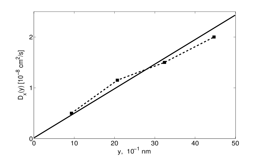
To show that the model presented does make sense, the comparison with direct measurements of inhomogeneous molecular diffusion in thin liquid film deposited on solid surface [2] is carried out. Let us first show, that the assumption of the linear dependence of the microscopic lateral diffusion coefficient on the distance from solid substrate holds. The least-square linear fit of the experimental data for lateral diffusion coefficients taken from [2] is presented Fig. 2. This fit justifies the assumption the approximate law for $D_{x}(y)$ with a rather good accuracy.

Figure 2: The linear fit of experimental data of Ref. [2] (Fig. 6b there; black squares corresponds to the same symbols in the cited source), which confirms the chosen dependence $D_{x}(y)=ky$ and allows to determine the tangent $k=0.4384\;\mathrm{cm^{2}/(s\cdot nm)}$.

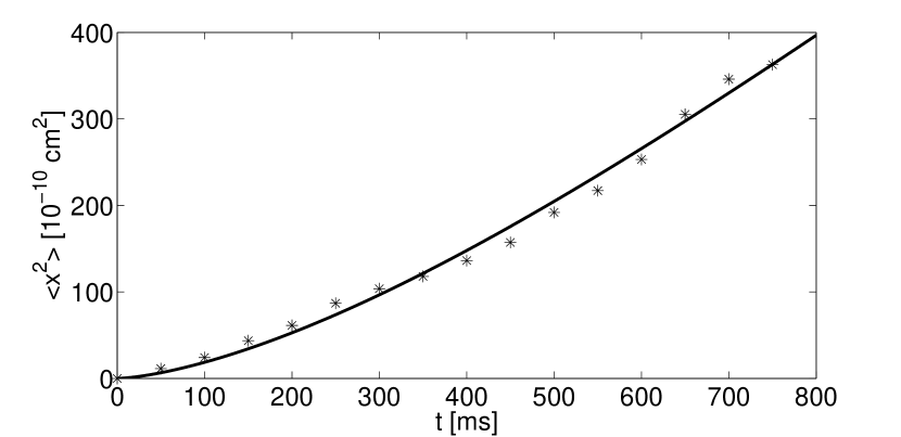
Using the value of the slope obtained, the calculation according to the formula (20) are completed for the experimental film thickness (note that the series (20) has a relatively fast convergence, e.g. the maximal relative difference between result presented by truncations at 11th and 10th terms is 2% and at between truncated 21th and 20th terms is 0.2%). Note, that the vertical component of diffusion coefficient is unknown from the direct measurements. Therefore, it is estimated in such a way that the resulting curve fits the experimental points, see Fig. 3. These experimental points represented as stars in Fig. 3. Note also that if one need to take into account 3D picture with two-dimensional lateral layers, the curves keep the same shape, but the adjustable parameter would be simple $\sqrt{2}$ times smaller. This follows from the Eqs. (8), (13).

The experimental points correspond to a single trajectory from the set of the overall 4 trajectories kindly provided by authors of Ref. [2]. For all of them the behavior at short times (governed by practically deterministic process of the departure from the surface) is practically the same. For longer observation times, the individual trajectories show various fluctuation features like large excursions and returns, and the averaging over our very restricted sample does not produce better results than taking an individual one. We use the trajectory, MSD of which corresponds to most regular curve over the time interval considered.

The considered time range allows to cover two specific regimes: i) During the interval from 0 to approximately 400 ms, the process is superdiffusive MSD ($<x^{2}>\sim t^{3/2}$). It coincides with the analytically exact superdiffusion obtained for semi-infinite region. The natural reason for this is that at short times a walker can not approach the upper boundary of film. Thus there is no sufficient difference between solutions as well as for physical experimental picture. ii) The transient process from superdiffusion to normal diffusion starting from time approximately 400 ms. Within this subinterval, the MSD curve can not be represented as a power-law function, compare with the Fig. 1, however the series solution (20) adequately reproduces experimental data.

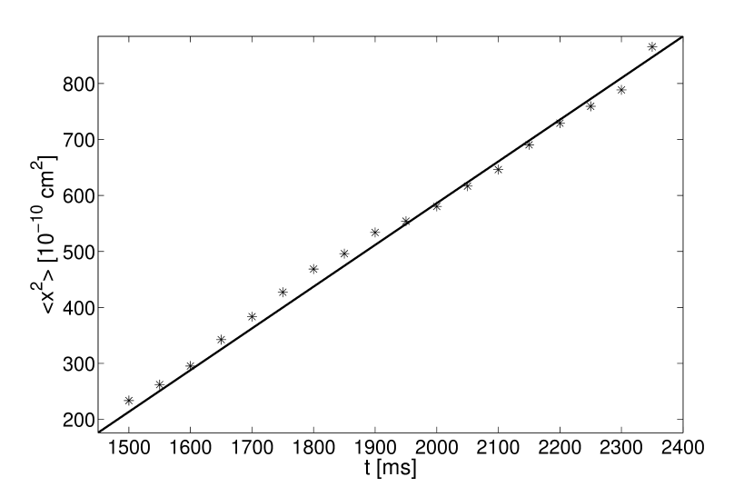
The asymptotic large-time MSD corresponding to the normal diffusion, see Fig. 1 for simulated curve and Fig. 4 confirming this conclusion by the experimental data. See also discussion of long observation times in [2].

Figure 3: The comparison of calculated curve of a mean-square-displacement (solid line) with experimental data (asterisks) provided by authors of [2] for short observation time. Parameters of the film: $H=17\;\mathrm{nm}$, $k=0.4384\;\mathrm{cm^{2}/(s\cdot nm)}$; vertical diffusion coefficients $D_{y}=8\cdot 10^{-13}\;\mathrm{cm^{2}/s}$ (or $8\cdot 10^{-13}/\sqrt{2}\;\mathrm{cm^{2}/s}$) for 3D case.

Thus, that anomalous diffusive behavior in lateral direction is caused by very weak vertical diffusion, i.e. rare jumps between layers: their rate is five orders of magnitude smaller then the lateral one.

Note also that our model deals with averaged motion. Correspondingly, it does not take into account fluctuations along individual trajectories, which are significant for large times of observation mirrored in growing fluctuations in $D$ [2]. Since the total number of trajectories obtained in the experiment is limited, and these trajectories show considerable differences between different runs, as they should. Fitting the results of a theory relying on ensemble-averaged quantities to this data is therefore connected with large statistical uncertainties, and one can mostly speak about trends, which are correctly captured by our theoretical description. The more convincing proof can be only given by performing more experiments in longer runs.

Figure 4: The comparison of calculated curve of a mean-square-displacement ($<x^{2}>_{\infty}\sim kHt$, see the Eq. (21). The constant vertical shift does not coincide with the analytical expression due to certain irregular markers’ jumps and stops during the experiment) with experimental data (asterisks) provided by authors of [2] for long observation time. Parameters of the film: $H=17\;\mathrm{nm}$, $k=0.4384\;\mathrm{cm^{2}/(s\cdot nm)}$; vertical diffusion coefficient $D_{y}=8\cdot 10^{-13}\;\mathrm{cm^{2}/s}$ (or $8\cdot 10^{-13}/\sqrt{2}\;\mathrm{cm^{2}/s}$ for 3D case).

5 Additional discussion

One of our basic simplifications is based on the assumption of a constant vertical diffusion coefficient coexisting with height-dependent lateral one. However, detailed studies of a near-wall motion of mesoscopic particles show that both components of the diffusion coefficient should depend on the distance from a wall, see the theoretical derivation and discussion in [7]. In this case the explicit $y$-dependence of the vertical diffusion coefficient should be taken into account, and Eq. (3) should be replaced by a more general one

$$\frac{\partial p}{\partial t}=D_{x}(y)\frac{\partial^{2}p}{\partial x^{2}}+\frac{\partial}{\partial y}D_{y}(y)\frac{\partial p}{\partial y}.$$ (22)

(If starting on the Langevin level, the kinetic (Hanggi-Klimontovich) interpretation of the Langevin equation for vertical motion should be used when assuming that the equilibrium distribution of the molecules in $y$-direction is homogeneous [17]). Although Eq. (22) is more complex than our initial Eq. (3), the assumption of independence of motion in $y$ on the lateral position and thus the conditional independence and the factorization of $x$- and $y$-motions still hold.

Now, let us subdivide the vertical diffusion coefficient in (22) into a constant and a variable parts: $D_{y}(y)=D_{y}^{(c)}+D_{y}^{(v)}(y)$. Then the Eq. (5) takes the form:

$$\frac{\partial p_{y}}{\partial t}=\left(D_{y}^{(c)}+D_{y}^{(v)}(v)\right)\frac{\partial^{2}p_{y}}{\partial y^{2}}+\frac{\partial D_{y}^{(v)}}{\partial y}\frac{\partial p_{y}}{\partial y}$$ (23)

Supposing that $D_{y}^{(v)}<<D_{y}^{(c)}$ we can neglect the second term in brackets in the first term in the right hand side of this equation (in a factor in front of the second derivative) and conclude that the coordinate dependence of $D_{y}$ mainly leads to the emergence of a drift term in $y$-direction. The last one actually changes the motion from a pure Brownian one to a combination of diffusion and regular drift. These results in a change of the effective MSD-exponent in $y$ from 1.5 closer to 2 during the first stage but does not influence the late stage of the process: after a uniform redistribution of walkers over a bulk the averaged lateral MSD will correspond to the normal diffusion. The numerical solution of (23) with $D_{y}^{(v)}(y)=0.05\div 0.2D_{y}^{(c)}y$ shows that initial superdiffusion in this case is sufficiently faster than the experimentally observed one, and moreover that the transient to a normal diffusion is shorter. In fact the resulting process comprises short-time regular ballistic drift ($\left<x^{2}\right>\sim t^{2}$) leading to the uniform filling of the layer with succeeding normal lateral diffusion.

Thus, the assumption of uniform small vertical diffusion coefficient can be considered as adequate for the description of the observed pattern of lateral diffusion for extremely small tracers, confirming the supposition made in [3]. The additional confirmation of this assumption can be found in the work [18], where the interpretation of experiments is provided. Authors argued that the microscopic molecular picture of media corresponds to the layered structure with small probability of jumps of molecules (nanometer scale objects) between adjacent layers. Our model discussion confirms these conclusions.

6 Summary

We considered lateral diffusion of a particle in a layered ultrathin fluid medium and obtained the solutions for the lateral mean-square-displacement. The results demonstrate the transition from superdiffusion at short times to asymptotically normal diffusion, as is confirmed by the experimental findings.

From the theoretical point of view, our work discusses an interesting case when the Batchelor’s equation in 1D appears to be exact, emerging from the full two-dimensional Fokker-Plank equation due to conditional independence of motions along both coordinates. Note that these conditionally independent motions are still connected via the common parameter: the time.

References

- [1] M. A. Bevan, D. C. Prieve, Hindered diffusion of colloidal particles very near to a wall: Revisited, J. Chem. Phys. 113 (2000) 1228–1236. doi:10.1063/1.481900.
- [2] J. Schuster, F. Cichos, C. von Borzcyskowski, Diffusion in ultrathin liquid films, European Polymer Journal 40 (2004) 993–999. doi:10.1016/j.eurpolymj.2004.01.031.
- [3] K. D. Kihm, A. Banerjee, C. K. Choi, T. Takagi, Near-wall hindered Brownian diffusion of nanoparticles examined by three-dimensional ratiometric total internal reflection fluorescence microscopy (3-D R-TIRFM), Experiments in Fluids 37 (2004) 811–824. doi:10.1007/s00348-004-0865-4.
- [4] A. Banerjee, K. D. Kihm, Experimental verification of near-wall hindered diffusion for the Brownian motion of nanoparticles using evanescent wave microscopy, Phys. Rev. E 72 (2005) 042101. doi:10.1103/PhysRevE.72.042101.
- [5] P. Huang, K. S. Breuer, Direct measurement of anisotropic near-wall hindered diffusion using total internal reflection velocimetry, Phys. Rev. E 76 (2007) 046307. doi:10.1103/PhysRevE.76.046307.
- [6] P. Sharma, S. Ghosh, S. Bhattacharya, A high-precision study of hindered diffusion near a wall, Appl. Phys. Lett. 97 (2010) 104101. doi:10.1063/1.3486123.
- [7] J. Happel, H. Brenner, Low Reynolds Number Hydrodynamics, Kluwer Academic Publishers Group, Dordrecht, The Netherlands, 1983.
- [8] M. D. Carbajal-Tinoco, R. Lopez-Fernandez, J. L. Arauz-Lara, Asymmetry in colloidal diffusion near a rigid wall, Phys. Rev. Lett. 99 (2007) 138303. doi:10.1103/PhysRevLett.99.138303.
- [9] G. I. Taylor, Diffusion by continuous movements, Proc. London Math. Soc. 20 (1922) 196–212. doi:10.1112/plms/s2-20.1.196.
- [10] G. Matheron, G. De Marsily, Is transport in porous media always diffusive? A counterexample, Water Resour. Res. 16 (1980) 901–917. doi:10.1029/WR016i005p00901.
- [11] E. A. Novikov, Concerning a turbulent diffusion in a stream with a transverse gradient of velocity, J. Appl. Math. and Mech. 22 (1958) 412–414. doi:10.1016/0021-8928(58)90074-1.
- [12] E. Ben-Naim, S. Redner, D. ben Avraham, Bimodal diffusion in power-law shear flows, Phys. Rev. A 45 (1992) 7207–7213. doi:10.1103/PhysRevA.45.7207.
- [13] E. B. Postnikov, Hierarchical mean-field model describing relaxation in a small-world network, Phys. Rev. E 80 (2009) 062105. doi:10.1103/PhysRevE.80.062105.
- [14] J. Sancho, M. Miguel, D. Durr, Adiabatic elimination for systems of brownian particles with non-constant damping coefficients, J. Stat. Phys. 28 (1982) 291–305.
- [15] A. P. Dawid, Conditional independence in statistical theory, J. R. Stat. Soc., Ser. B 41 (1979) 1–39.
- [16] G. K. Batchelor, Diffusion in a field of homogeneous turbulence, Math. Proc. Cambridge Phil. Soc. 48 (1952) 345–362. doi:10.1017/S0305004100027687.
- [17] I. M. Sokolov, Ito, Stratonovich, Hanggi and all the rest: The thermodynamics of interpretation”, Chem. Phys. 375 (2010) 359–363. doi:10.1016/j.chemphys.2010.07.024.
- [18] J. Schuster, F. Cichos, C. von Borzcyskowski, Anisotropic diffusion of single molecules in thin liquid films, Eur. Phys. J. E 12 (2003) 75–80. doi:10.1140/epjed/e2003-01-019-y.