Segregation and phase inversion of strongly and weakly fluctuated Brownian particle mixtures in spherical containers

Abstract

We investigate the segregation pattern formations of strongly and weakly fluctuated Brownian particle mixtures, which are confined in spherical containers with finite volumes. We consider systems where the container restricts the motions of particles combining two familiar methods: spherically symmetric linear potential and the container edge wall. In such systems, the following two segregation patterns are observed. When the container radius is large enough, more weakly fluctuated particles accumulate around the center of the container than strongly fluctuated particles. On the other hand, inverted distributions of strongly and weakly fluctuated particles are observed when the container radius is small. We also found a similar segregation and phase inversion if such particle mixtures construct a chain (hetero-fluctuated polymer) and are confined in a container with no linear potential. We provide the qualitative mechanism and the relationships for the biopolymer behaviors of such phase inversions.

Recently, the formation of spatially ordered patterns of self-propelled populations such as bio-molecules, cells, animals, and artificial autonomous motors have been extensively studied rev1 ; nagai0 ; nagai00 ; nagai ; cell1 ; cell2 ; cell3 ; cell4 ; cell5 ; awa ; animal1 ; animal2 ; animal3 ; animal4 ; midori ; nakata1 ; nakata2 ; nakata3 ; nakata4 ; active1 ; active2 ; ganai . Theoretical studies using idealized models have provided several insights for the understanding of physical, biological, and social phenomena.

Segregation patterns of particles involving different characteristics such as size, shape, stiffness, and mobility are typical examples of pattern formations that have been universally observed in nonequilibrium systems cell1 ; cell2 ; cell3 ; active1 ; active2 ; ganai ; kona1 ; kona2 ; kona3 ; kona4 ; kona5 . In most of these studies, the primary focus is on the contributions of inhomogeneous particles in bulk systems. On the other hand, in real systems, several objects are usually confined in a limited space. For example, bio-molecules in cells are often confined in subcellular organelles, and the structural stability and reaction activities of bio-molecules are much different between in vivo and in vitro situationsganai ; crowd1 ; crowd2 ; crowd3 ; Aoki ; Fujii . During the developmental processes of multi-cellular organisms, each cell migrates in the restricted space in their host bodyhassei . Moreover, the segregation patterns of granular mixtures are also highly influenced by the form and the size of the containerkona2 ; kona4 . Thus, to uncover pattern formations mechanisms in real nonequilibrium systems, the influence of container characteristics should also be clarified.

In this letter, through simple nonequilibrium particle models, we investigate the influence of the container characteristics, in particular container size, on the segregation patterns. First, we consider the segregations of hetero-Brownian particles model consisting of finite volume particles driven by different magnitude fluctuations. This model is considered to be one of the simplest descriptions of active and inactive self-propelled particle mixtures. We focus on the segregation pattern of strongly and weakly fluctuated particles under container restrictions given by the combination of two familiar effects: spherically symmetric linear potential in the bulk and a wall at the edge of the container.

In addition, we consider the hetero-fluctuated polymer, which is a chain constructed by hetero-Brownian particles in a spherical container without a linear potential. Such polymers are regarded to be a simplified chromosome model for nuclei involving transcriptional active and inactive (silenced) regionsganai . Here, the regions containing strongly fluctuated particles are considered to be transcriptional active regions because several proteins such as chromatin remodeling factors and transcription factors often access such DNA regions and produce several mechanical perturbations through the ATP hydrolysis energy consumption. Then, by focusing on the container size dependent behaviors of this model, we understand the possible contributions of bio-molecule confinement in biological activities.

We now introduce the model for hetero-Brownian particles and a hetero-fluctuated polymer in a container. These systems consist of $N$ spherical particles with the common diameters of $d$. Particles are driven by random forces, which have different average magnitudes for each respective particle. Then, the equation of the motion of each particle is given by

$${\bf\dot{x}_{i}}=-\nabla_{i}(V_{int}(\{{\bf x}_{i}\})+V_{con}(\{{\bf x}_{i}\}))+{\bf\eta}_{i}(t),$$ (1)

$$<{\bf\eta}_{i}(t){\bf\eta}_{i}(t^{\prime})>=2G_{i}\delta(t-t^{\prime}),$$ (2)

where ${\bf x}_{i}$ is the position of the $i$th particle, ${\bf\eta}_{i}$ and $G_{i}$ are the random force working on the $i$th particle and its magnitude, respectively. Here, the origin (${\bf x}_{i}=0$) is the center of the container.

The interaction potential between particles is indicated by $V_{int}(\{{\bf x}_{i}\})$. Due to the excluded volumes of particles in the hetero-Brownian particle model, we only consider the soft-core repulsive potential as $V_{int}(\{{\bf x}_{i}\})=V^{sf}(\{{\bf x}_{i}\})$, where

$$V^{sf}(\{{\bf x}_{i}\})=\sum_{i<j}\begin{cases}\frac{k_{e}}{2}(|{\bf x}_{i}-{\bf x}_{j}|-d)^{2}\,\,\,\,\,\,(|{\bf x}_{i}-{\bf x}_{j}|<d)\\ 0\,\,\,\,\,\,(Otherwise)\end{cases},$$ (3)

with the elastic constant $k_{e}$. In the hetero-fluctuated polymer model, we assume that chain of Brownian particles does not have branches. Then, we have $V_{int}(\{{\bf x}_{i}\})=V^{sf}(\{{\bf x}_{i}\})+V^{ch}(\{{\bf x}_{i}\})$, where

$$V^{ch}(\{{\bf x}_{i}\})=\sum_{i}\frac{k_{c}}{2}(|{\bf x}_{i}-{\bf x}_{i+1}|-d)^{2}$$ (4)

with constants $k_{e}$ and $k_{c}$.

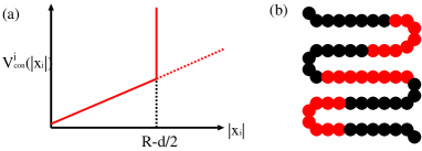
The potential for the container spatial constraints is given by $\displaystyle V_{con}(\{{\bf x}_{i}\})$. In this letter, we consider $\displaystyle V_{con}(\{{\bf x}_{i}\})=\sum_{i}V^{i}_{con}({\bf x}_{i})$, where $V^{i}_{con}$ is given by sum of the potential of the wall at the edge of container $V^{i}_{wall}$ and the linear potential in the bulk $V^{i}_{bulk}$ (see Fig. 1(a)) as

$$V^{i}_{wall}({\bf x}_{i})=\begin{cases}\frac{k_{w}}{2}(|{\bf x}_{i}|-(R-\frac{d}{2}))^{2}\,\,\,\,\,\,(|{\bf x}_{i}|>R-\frac{d}{2})\\ 0\,\,\,\,\,\,(Otherwise)\end{cases}$$ (5)

and

$$V^{i}_{bulk}({\bf x}_{i})=k_{l}|{\bf x}_{i}|$$ (6)

with constants $k_{w}$, $k_{l}$, and container radius $R$.

We now focus on the simplified systems containing only two types of particles: strongly fluctuated particles (S-particles) with $G_{i}=G_{s}$ and weakly fluctuate particles (W-particles) with $G_{i}=G_{w}$. Here, we give the number of S- and W-particles as $N/2$, $G_{s}=1$, $G_{w}=0$, $k_{e}=k_{c}=1024$, $d=1$, and $k_{l}$ holding $G_{s}/k_{l}>>d^{2}$. Even when $G_{w}>0$, we qualitatively obtain the same results as the case when $G_{w}<<G_{s}$ holds. In a hetero-fluctuated polymer, we also assume that the S- and W-particles are periodically connected where the length of each S- and W-particles region is $L/2$ (see Fig. 1).

Figure 1: (Color online) (a) Illustration of the container potential. (b) Illustration of hetero-fluctuated polymers where the black and gray (red) circles indicate weakly and strongly fluctuated particles, respectively.

Figure 2: (Color online) Typical snapshots of the distributions of S-particles (grey (red)) and W-particles (black) of hetero-Brownian particles model (N=512) on the 2-D cross section for (a) $R=10$, (b) $R=5$, and (c) $P(r)$ for typical $R$.

First, we focus on the segregation pattern formations of hetero-Brownian particles in the container. In the case of $k_{l}>0$ and $k_{w}=0$, W-particles (S-particles) tend to locate near (far from) the container center, which may be easily expected by considering the $G_{i}$-dependent distribution of particles affected by the potential. On the other hand, if there exists a hard wall at the edge of the container, the steady state properties of the system changes as follows.

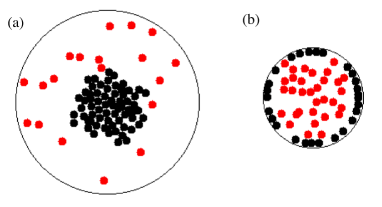
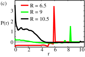
Figures 2(a) and 2(b) show typical snapshots of the S- and W-particle distributions in the 2-D cross section (particles at $-d/2\leq x\leq d/2$ on the $x-y-z$ space are shown) for $R=11$ and $R=6$, respectively. Figure 2(c) shows the relative radial distributions $P(r)$ for some $R$ with $k_{l}=0.01$, $k_{w}=1024$, and $N=512$. Here, $P(r)$ is given as $P_{w}(r)-P_{s}(r)$, where $P_{m}(r)=n_{m}(r)/4\pi r^{2}$ ($m=$ S or W) are the respective radial particle distributions, $r$ is the distance from the origin, and $n_{m}(r)$ is the frequency of $m$-particles in the region between $r$ and $r+dr$ ($dr=0.1$ is employed). As shown in these figures, the distributions of S- and W-particles are highly influenced by $R$: more W-particles are distributed around the center than S-particles for large enough $R$, while the inverted distribution occurs for small $R$.

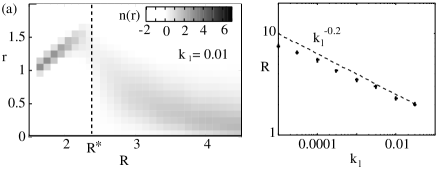
The phase inversions are independent of $k_{l}$, $D_{s}$, and $N$ even though the $R$ value at which phase inversion occurs ($R^{*}$) depends on these values. To understand these dependencies, we study the simplest possible system with $N=2$, which contains one S-particle and one W-particle. Figure 3(a) shows $n(r)=n_{w}(r)-n_{s}(r)$ shuusoku for several $R$ with $k_{l}=0.01$, while Fig. 3(b) shows $R^{*}$ as a function of $k_{l}$. Here, $R^{*}$ is given as the maximum $R$ with the peak of $n(r)$ near the edge of container. As shown in these figures, $R^{*}$ is given by $\sim k_{l}^{-1/5}$.

To consider the mechanism of such results, we first examine the case $k_{l}=0$. In this case, the motions of W-particles are driven only by collisions with S-particles. Then, once W-particles reach the edge wall, the S-particle forces acts only in the direction from the center to the outer wall. Thus, the W-particles tend to stay at the edge wall independent of $R$.

Based on the above fact, $R^{*}$ is roughly estimated as follows. For simplicity, we assume $D_{s}$ is so large compared to $k_{l}R$ that the influence of the linear potential is negligible for S-particles. Basically, the W-particles tend to move to the container center with velocity $k_{l}$ by the influence of the linear potential. However, the W-particles tend to move to the edge of the container if the S- and W-particles collide frequently. The collision rate between S- and W-particles is proportional to two values: the volume fraction of particles (order $(d/R)^{-3}$) and the inverse of the time that the S-particles entire the space (order $G_{s}R^{-2}$). Here, we assume that the average distance of the W-particle’s outward-directed movements during a single collision is $\lambda$. Then, W-particles tend to move to the container edge if the collision rate is so large that $d^{3}G_{s}R^{-5}\lambda>k_{l}$, which indicates $R^{*}\sim(d^{3}G_{s}\lambda/k_{l})^{1/5}$.

We obtained similar results if $V^{i}_{bulk}$ is a harmonic potential. However, if $V^{i}_{bulk}$ is given by $~{}(|{\bf x_{i}}|/R_{o})^{n}$ with a large $n$, more S-particles tend to occupy the interior positions of the container than W-particles independent of $R$ and $R_{o}$ because $V^{i}_{bulk}$ is regarded as the potential indicating a wall exists at $|{\bf x_{i}}|=R_{o}+d/2$.

Figure 3: (a) $n(r)$ for several $R$ with $k_{l}=0.01$, and (b) $R^{*}$ as a function of $k_{l}$ for $N=2$ with dashed curve indicating $R^{*}=k_{l}^{-1/5}$.

Figure 4: (Color online) Typical snapshots of the distributions of S-particles (grey (red)) and W-particles (black) of the hetero-fluctuated polymer model (N=512) on the 2-D cross section for (a) $R=11$ and (b) $R=6$ with $L=64$, and $P(r)$ of this model for typical $R$ with (c) $L=64$ and (d) $L=128$.

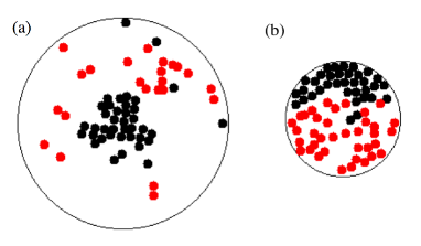
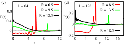
Next, we focus on the segregations of S- and W-particles constructing the hetero-fluctuated polymer in the spherical box ($k_{l}=0$ and $k_{w}=1024$). In the following, we focus on the cases of $L=32,64,128$ for $N=512$, respectively. Figures 4(a) and 4(b) show typical snapshots of the particle distributions on the 2-D cross-section with $L=64$ for $R=11$ and $R=6$, respectively, and Fig. 4(c) and 4(d) show the relative radial distribution functions of steady state S- and W-particles for some $R$ with $L=64$ and $L=128$, respectively. As shown in these figures, more W-particles tend to be distributed at the container center than S-particles for large enough $R$. On the other hand, W-particles tend to be distributed near the edge of the container for small $R$.

In a recent study, the latter type of segregation pattern was observed as ”activity-based segregation” in a similar model ganai . On the other hand, the present result indicates the patterns induced by the segregations generally depends on the container size. We found that phase inversion occurs at $R=9\sim 10$ in the case of $L=64$ and at $R=13\sim 14$ in the case of $L=128$. We also found that the latter segregation pattern does not appear when $L=32$. Then, these results indicate phase inversion occurs at $R\sim(dL/2)^{3/5}+d$ only if $L$ is large enough. We found almost the same results in the cases of $N=256$ and $1024$.

In order to qualitatively explain the present phase inversions, we propose the following scenario. In general, the Brownian motion of a chain induces the entropic force (rubber elasticity), which works on each chain element to promote chain assembly.

In an equilibrium system, the elasticity of effective force is proportional to the temperature. However, the hetero-fluctuated polymer consists of particles with large and small fluctuations with $G_{s}$ and $G_{w}$, respectively, that is equivalent to chains containing parts with high and low temperatures. Then, the effective elasticity for each particle seems to be influenced by both $G_{s}$ and $G_{w}$. Here, it seems natural that the magnitude of the elasticity for $i$th particle is proportional to $G_{i}^{*}$, which depends on $i$ but always holds for $G_{w}<G_{i}^{*}<G_{s}$.

Then, if we can neglect the effects of the excluded particle volume and the edge wall of the container, the radial distribution of the S- and W-particles is approximately obtained by a 3-D Gaussian distribution around the polymer center of the mass with the variance proportional to $G_{s}/G_{i}^{*}$ and $G_{w}/G_{i}^{*}$, respectively. Even when each particle has the finite volume, the diversity of the S- and W-particles distributions highly correlates with $G_{s}/G_{i}^{*}$ and $G_{w}/G_{i}^{*}$, respectively. Thus, if $R$ is large enough, more W-particles are located near the center of the polymer than S-particles since $G_{w}/G_{i}^{*}<1<G_{s}/G_{i}^{*}$ holds for all $i$.

The above arguments indicate that W-particles (S-particles) tend to be distributed near (far from) the container center because the center of mass of the polymer tends to close to the container center. Moreover, when $R$ is sufficiently large, the distance between a particle at the center of S-particle region and that of the neighboring W-particle regions is estimated $\sim(dL/2)^{3/5}$ on average by the arguments of self-avoiding random walk dojan . Then, when $R<(dL/2)^{3/5}$, the S- and neighboring W-particle regions tend to collide excessively with each other while the force assembling the regions becomes weaker. In such cases, the W-particles tend to move to the edge of the container by similar mechanisms with those obtained in the hetero-Brownian particle system.

If the volume fraction of the polymer is close to that of the closed packing, some corrections are needed to this arguments. However, the volume fractions of our simulations ($N=256,512$ and $1024$) are considered small enough when $R\sim(dL/2)^{3/5}$. Thus, the phase inversion $R$ seems insensitive for $N$ in our simulations.

In this letter, we investigated the segregation patterns of strongly and weakly fluctuated Brownian particles confined in a spherical container. We found that the segregation patterns of such systems drastically depend on the container. Thus, in order to uncover the universal and individual aspects of several nonequilibrium particle populations, we should consideration of the effects of several containers.

The size of the cell nucleus depends on the type and the developmental stage of the cell, even though the chromosome volume in each cell is the same. Then, the results of the presented polymer model provide some insights into cell type-dependent chromosome behaviors. On the other hand, for pattern formations of a confined chain, we also note that the elasticity and the heterogeneity of the chain play important roleshermann ; pcook . Then, for more detailed arguments for the intra-nucleus chromosome structures, we will consider the hetero-fluctuated polymer model with further modifications by referencing recent studies.

The author is grateful to T. Sugawara, S. Shinkai, S. Lee, T. Sakaue and H. Nishimori for fruitful discussions and useful information. This research was supported in part by the Platform for Dynamic Approaches to Living System from the Ministry of Education, Culture, Sports, Science and Technology, Japan, and the Grant-in-Aid for Scientific Research on Innovative Areas (Spying minority in biological phenomena (No.3306) (24115515)) of MEXT of Japan.

References

- (1) T. Vicsek and A. Zafeiris, Physics Reports 517, 71 (2012).
- (2) V. Schaller et al., Nature 467, 73 (2010).
- (3) T. Butt et al., J. Biol. Chem. 285, 4964 (2010).
- (4) Y. Sumino et al., Nature 483, 448 (2012).
- (5) P. L. Townes and J. Holtfreter, J. Exp. Zool. 128, 53 (1955).
- (6) M. S. Steinberg, Curr. Opin. Gen. Dev. 17, 281 (2007).
- (7) F. Graner and J. A. Glazier, Phys. Rev. Lett. 69, 2013 (1992).
- (8) R. M. H. Merks and J. A. Glazier, Physica A 352, 113 (2005).
- (9) B. Szabó et al., Phys. Rev. E 74, 061908 (2006).
- (10) A. Awazu, Phys. Rev. E 76, 055101(R) (2007).
- (11) T. Vicsek et al., Phys. Rev. Lett. 75, 1226 (1995).
- (12) N. Shimoyama et al., Phys. Rev. Lett. 76, 3870 (1996).
- (13) C. Becco et al., Physica A 367, 487 (2006).
- (14) M. Ballerini et al., Proc. Natl. Acad. Sci. USA 105, 1232 (2008).
- (15) N. J. Suematsu et al., J. Phys. Soc. Jpn. 80, 06400 (2011).
- (16) N. J. Suematsu et al., Phys. Rev. E 81, 056210 (2010).
- (17) E. Heisler et al., Phys. Rev. E 85, 055201 (2012).
- (18) Y. S. Ikura et al., Phys. Rev. E 88, 012911 (2013).
- (19) A. E. Turgut et al., Swarm Intelligence 2, 97 (2008).
- (20) S. R. McCandlish, A. Baskaran, and M. F. Hagan, Soft Matter 8, 2527 (2012).
- (21) Y. Fily and M. C. Marchetti, Phys. Rev. Lett. 108, 235702 (2012).
- (22) N. Ganai, N. Sengupta, and G. I. Menon, Nuc. Aci. Res. 42, 1 (2014).
- (23) A. Wysocki and H. Lowen, Phys. Rev. E 79, 041408 (2009).
- (24) J. B. Knight et al., Phys. Rev. Lett. 70, 3728 (1993).
- (25) A. Awazu, Phys. Rev. Lett. 84, 4585 (2000).
- (26) A. Awazu, J. Phys. Soc. Jpn. 72, 1832 (2003).
- (27) M. Fujii et al., Phys. Rev. E 85, 041304 (2012).
- (28) F. Takagi et al., Proc. Natl. Acad. Sci. USA 100, 11367 (2003).
- (29) D. Kilburn et al., J. Am. Chem. Soc. 132, 8690 (2010).
- (30) J. Lin et al., Mol. Cell. Biol. 29, 2082 (2009).
- (31) K. Aoki et al., Proc. Natl. Acad. Sci. USA 108, 12675 (2011).
- (32) M. Fujii et al., PLoS ONE 8, e62218 (2013).
- (33) J. Slack, Essential Developmental Biology, 2nd ed. (Blackwell Publishing, Ltd., Oxford, 2006).
- (34) Here, is employed instead of because the convergence of is slow and numerically unstable for small in cases of small .
- (35) P.-G. de Gennes, Scaling Concepts in Polymer Physics (Cornell University Press, London, 1979).
- (36) N. Stoop et al., Phys. Rev. Lett. 106, 214102 (2011).
- (37) K. Finan, P. R. Cook, and D. Marenduzzo, Chromosome Res. 19, 53 (2011).