Derivation of Quantum Theory from Feynman’s Rules
Abstract
Feynman’s formulation of quantum theory is remarkable in its combination of formal simplicity and computational power. However, as a formulation of the abstract structure of quantum theory, it is incomplete as it does not account for most of the fundamental mathematical structure of the standard von Neumann–Dirac formalism such as the unitary evolution of quantum states. In this paper, we show how to reconstruct the entirety of the finite-dimensional quantum formalism starting from Feynman’s rules with the aid of a single new physical postulate, the no-disturbance postulate. This postulate states that a particular class of measurements have no effect on the outcome probabilities of subsequent measurements performed. We also show how it is possible to derive both the amplitude rule for composite systems of distinguishable subsystems and Dirac’s amplitude–action rule, each from a single elementary and natural assumption, by making use of the fact that these assumptions must be consistent with Feynman’s rules.
pacs:
03.65.-w, 03.65.Ta, 03.67.-aI Introduction
The mathematical formalism of quantum theory has numerous structural features, such as its use of complex numbers, whose physical basis has long been regarded as obscure. In recent years, there has been a growing interest in deriving these features from compelling physical principles inspired by an informational perspective on physical processes Wheeler (1990); Zeilinger (1999); Fuchs (2002); Grinbaum (2007). The purpose of such derivation is to better understand the differences between quantum and classical physics, to establish the range of validity of the various parts of the quantum formalism, and to identify physical principles whose validity might extend beyond quantum theory itself. Substantial progress has now been made, both in deriving much of the quantum formalism from physical principles Hardy (2001); Clifton et al. (2003); D’Ariano (2007); Goyal (2010); Reginatto (1998); Goyal et al. (2010); Chiribella et al. (2011); Masanes and Müller (2011); Dakic and Brukner (2011), and in identifying physical principles that account for some of the nonclassical features of quantum physics Barrett (2007); Pawlowski et al. (2009).
Almost without exception, the above-mentioned attempts to understand the quantum formalism have focussed their attention on the standard Dirac–von Neumann formalism. However, Feynman’s formulation of quantum theory provides a strikingly different representation of quantum physics Feynman (1948); Feynman and Hibbs (1965), and this raises the important question of whether we may be able to gain valuable insights by deriving quantum theory from Feynman’s perspective.
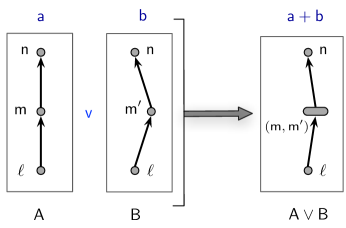
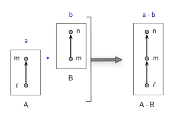
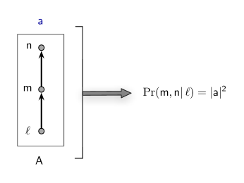
Perhaps the most remarkable feature of Feynman’s formulation is its formal simplicity. The simplicity is achieved by dispensing with the notion of the state of a system and with operators that represent measurements and temporal evolution or symmetry transformations. Instead, the primary notion is that of a transition of a system from one measurement outcome, obtained at some time, to another measurement outcome, obtained at some other time; and a complex-valued amplitude is associated with each transition. Feynman’s abstract formalism for individual systems consists of what we shall refer to as Feynman’s rules Feynman (1948). These rules, summarized in Fig. 3, stipulate how amplitudes associated with given transitions of a system are combined to yield amplitudes of more complex transitions of that system, and how probabilities are computed from amplitudes.
As Feynman observed, the rules for combining amplitudes bear a striking resemblance to the rules of probability theory Feynman (1948); Feynman and Hibbs (1965). In previous work Goyal et al. (2010), we seized on this observation to derive Feynman’s rules using a method similar to that used by Cox to derive the rules of probability theory from Boolean algebra Cox (1946, 1961). Our derivation provides a particularly clear understanding of why complex numbers are such a fundamental part of the mathematical structure of quantum theory, and provides a precise understanding of the relationship between Feynman’s rules and probability theory Goyal and Knuth (2011).
Feynman’s rules, however, do not, by themselves, constitute a complete formulation of quantum theory. Most importantly, they do not account for most of the fundamental mathematical structure of the standard von Neumann–Dirac formalism Dirac (1930); von Neumann (1955). For example, a basic property of the standard formalism is that state evolution is unitary, but this property does not follow from Feynman’s rules. While it is true that Feynman’s rules imply unitarity given the form of the classical action and Dirac’s amplitude–action rule Feynman (1948); Johnson and Lapidus (2000), unitarity does not follow as a direct consequence of Feynman’s rules alone, a problem of which Feynman was aware 111In Ref. Feynman (1948), Sec. 11, Feynman states, “One of the most important characteristics of quantum mechanics is its invariance under unitary transformations…. Of course, the present formulation, being equivalent to ordinary formulations, can be mathematically demonstrated to be invariant under these transformations However, it has not been formulated is such a way that it is physically obvious that it is invariant”.. Not only is this unsatisfactory on a theoretical level, it is particularly problematic since a corresponding classical action does not always exist for a quantum system Feynman and Hibbs (1965), and, even when one does exist, a mathematically rigorous proof of unitarity on the basis of Feynman’s path integral, assuming a general form for the action, is highly nontrivial Johnson and Lapidus (2000).
Even more fundamentally, the notion of a quantum state itself does not follow naturally from Feynman’s rules. Contrary to what is asserted in Refs. Feynman (1948); Feynman and Hibbs (1965), one cannot simply assume that the state of a system consists of the amplitudes to obtain the possible outcomes of a given measurement irrespective of the prior history of the system, for two reasons. First, one cannot exclude the possibility that the system is entangled with another system, and is therefore in a mixed state rather than a pure state. Second, before these amplitudes can be declared to constitute the state of the system, one must establish that these amplitudes suffice to compute the outcome probabilities of not just the given measurement but of any measurement that could be performed on the system.
Thus, in order to complete the derivation of quantum theory from the Feynman perspective, it is essential to discover what physical ideas are needed in order to derive the standard quantum formalism given Feynman’s rules for individual systems. In this paper, we show that a single physical idea, formalized in the no-disturbance postulate, suffices. This postulate states that a particular class of measurements—which we refer to as trivial measurements—have no effect on the outcome probabilities of subsequent measurements. A trivial measurement has a single outcome, this outcome having been obtained by coarse-graining over all of the outcomes of an atomic, repeatable measurement (see Sec. II.1 for definitions of these terms). For example, a Stern-Gerlach measurement with but a single detector which registers all outgoing systems is a trivial measurement.
The no-disturbance postulate formalizes a key difference between classical and quantum physics. In quantum physics, a trivial measurement is non-disturbing. However, in classical physics, a trivial measurement is generally disturbing. For example, consider a trivial Stern-Gerlach measurement with a single coarse-grained outcome obtained by coarse-graining over two atomic outcomes. From a classical point of view, it is a fact of the matter that the system passed through one of the atomic outcomes, even though the coarse-grained outcome was not capable of registering this fact. As we show in Sec. III.1, this classical inference leads to a change in the outcome probabilities of subsequent measurements.
One can understand the no-disturbance postulate quite naturally as follows. From an information-theoretic point of view, it is the gain of information about a quantum system that is ultimately responsible for the disturbance of its state Fuchs and Peres (1996). From this viewpoint, it seems eminently plausible that, conversely, there should exist measurements that provide no useful information which do not disturb the state 222I am grateful to Paulo Perinotti for suggesting this point of view.. Informally, one might say that, if a measurement provides no information, then it need not disturb the state of the system 333One cannot rule out measurements that provide no useful information and yet still disturb the state.. Since a trivial measurement has only one outcome, one gains no information (in the sense of Shannon information) about which outcome was obtained on learning the outcome of the measurement. This is similar to ones predicament on learning that a two-headed coin has landed heads. The no-disturbance postulate asserts that trivial measurements are such non-disturbing, non-informative measurements.
Since the no-disturbance postulate exposes a fundamental difference between classical and quantum physics, it is an excellent candidate to take as a physical postulate in deriving quantum theory. Indeed, we have previously employed a special case of this postulate in our derivation of Feynman’s rules Goyal et al. (2010), and a very similar idea has more recently been employed in Ref. Pfister and Wehner (2013) to derive interesting results regarding the state space of general probabilistic theories.
As mentioned above, Feynman’s rules concern a given quantum system, so that additional rules must be given if one wishes to treat composite systems of distinguishable or indistinguishable subsystems. A particularly attractive feature of these rules is their formal simplicity. In Ref. Feynman and Hibbs (1965), the amplitude rules for such composite systems are simply postulated, presumably having been extracted from the standard formalism. In this paper, we show that the rule for composite systems of distinguishable subsystems can in fact be derived from a simple composition postulate on the condition that Feynman’s rules for individual systems are valid. The composition postulate simply posits that the amplitude of a transition of a composite system consisting of two noninteracting subsystems is a continuous function of the amplitudes of the respective subsystem transitions. Remarkably, the rule for assigning amplitudes to composite systems is uniquely determined by the requirement that the amplitude assignment to the composite system be consistent with Feynman’s rules for assigning amplitudes to individual systems. This rule immediately gives rise to the tensor product rule in the standard quantum formalism. The derivation of the symmetrization postulate, which is needed to describe composite systems consisting of indistinguishable subsystems, is detailed elsewhere Goyal (2013).
Finally, a striking feature of Feynman’s formulation is its remarkably direct connection to the Lagrangian formulation of classical physics. More precisely, when a series of transitions of a quantum system in configuration space is well approximated by a continuous trajectory of the corresponding classical system, Dirac’s amplitude–action rule associates the amplitude to the series of transitions, where is the action of the corresponding classical trajectory Dirac (1933). It is this rule from which much of the computational power of Feynman’s rules derives, allowing, for example, the derivation of the Schroedinger equation Feynman (1948) and quantum electrodynamics Feynman (1949). Dirac obtained this rule on the basis of a detailed analogy between transformations in quantum theory and contact transformations in the Lagrangian formulation of classical mechanics. However, given the fundamental importance of this classical–quantum connection, a simpler and more direct derivation is desirable. Here, using only elementary properties of the action, we provide a simple and direct derivation of this rule on the simple assumption that the amplitude of a path in configuration space is a continuous function of its classical action.
The work described here significantly improves upon previous attempts to address many of the above-mentioned issues. In particular, a previous attempt to derive unitarity from Feynman’s rules makes appeal to the Hilbert space norm, which itself must be independently justified Caticha (2000). In contrast, our derivation rests entirely on the no-disturbance postulate. Similarly, two previous derivations of the rule for composite systems of distinguishable subsystems implicitly assume that the functional relationships involved are complex-analytic, an assumption which significantly detracts from the physical transparency of the derivations Tikochinsky (1988); Caticha (1998). We are able to avoid such assumptions.
The results given here have implications for many issues which have been raised in the literature. For example, a recurrent question is whether linear temporal evolution can be replaced with nonlinear temporal evolution Pearle (1976); Bialynicki-Birula and Mycielski (1976); Shimony (1979); Weinberg (1989a, b). Such replacement has a variety of motivations, such as the desire to incorporate the quantum measurement process into the usual temporal evolution of a quantum state, or to solve the black hole information paradox Giddings (1995). Such work has led to attempts to explore whether, taking certain other parts of the quantum formalism as a given, one can derive linearity or unitarity from a physical principle such as the requirement that there is no instantaneous signaling between separated subsystems Simon et al. (2001); Ferrero et al. (2004, 2006). Our earlier derivation of Feynman’s rules, together with the present derivation of unitarity from the no-disturbance postulate, shows that the linearity and unitarity of temporal evolution is very basic to the structure of quantum theory, and cannot be replaced with nonlinear deterministic evolution, even in a manner that is barely experimentally perceptible, without undermining the entire edifice. Furthermore, since our derivation of unitarity depends only on no-disturbance, and not on any postulate that refers to the behavior (such as no instantaneous signaling) of composite systems, our result shows that such behavior, contrary to that which is suggested by some previous work Simon et al. (2001); Ferrero et al. (2004, 2006), is not necessary to understand unitarity.
The remainder of the paper is organized as follows. In Sec. II, we summarize the experimental framework and notation presented in Ref. Goyal et al. (2010), extend the framework to deal with composite systems, and summarize Feynman’s rules in operational language. In Sec. III, we formulate the no-disturbance postulate, and use this to systematically introduce the notion of a quantum state, show that states evolve unitarily, and show that repeatable measurements are represented by hermitian operators. In Sec. IV, we introduce a composition operator, formulate its symmetry relations, and show, via the composition postulate, that these lead to the amplitude rule for composite systems. Finally, in Sec. V, we derive Dirac’s amplitude–action rule. We conclude in Sec. VI with a discussion of the results and their broader implications.
II Background and Notation
II.1 Experimental Framework
An experimental set-up is defined by specifying a source of physical systems, a sequence of measurements to be performed on a system in each run of the experiment, and the interactions between the system and its environment which occur between the measurements (see example in Fig. 1). In a run of an experiment, a physical system from the source passes through a sequence of measurements , which respectively yield outcomes at times . These outcomes are summarized in the measurement sequence . In between these measurements, the system may undergo interactions with the environment. We shall label the possible outcomes of a measurement as as far as is needed in each case.
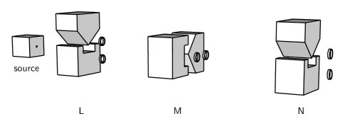
Over many runs of the experiment, the experimenter will observe the frequencies of the various possible measurement sequences, from which the experimenter can estimate the probability associated with each sequence. The probability associated with sequence is defined as the probability of obtaining outcomes conditional upon obtaining ,
| (1) |
A particular outcome of a measurement is either atomic or coarse-grained. An atomic outcome is one that cannot be more finely divided in the sense that the detector whose output corresponds to the outcome cannot be sub-divided into smaller detectors whose outputs correspond to two or more outcomes. An example of atomic outcomes are the two possible outcomes of a Stern-Gerlach measurement performed on a silver atom. A coarse-grained outcome is one that does not differentiate between two or more outcomes, an example being a Stern-Gerlach measurement where a detector’s field of sensitivity encompasses the fields of sensitivity of two detectors, each of which corresponds to a different atomic outcome. Abstractly, if a measurement has an outcome which is a coarse-graining of the outcomes labeled and of measurement , the outcome is labeled , and this notational convention naturally extends to coarse-graining of more than two atomic outcomes. In general, if all of the possible outcomes of a measurement are atomic, we shall call the measurement itself atomic. Otherwise, we say it is a coarse-grained measurement. A coarse-grained measurement with but a single outcome is called a trivial measurement as its outcome provides us with no more information than the fact that the measurement has detected a system at a particular time.
As explained in Refs. Goyal (2008); Goyal et al. (2010), the measurements and interactions which can be employed in a given experiment must satisfy certain conditions if they are to lead to a well-defined theoretical model. The measurements that are employed in an experimental set-up must be repeatable, come from the same measurement set, , or be coarsened versions of measurements drawn from this set; and the first measurement in each experiment must be atomic. These conditions ensure that (i) all the measurements are probing the same aspect (say, the spin behavior) of the system, and (ii) the outcome probabilities of all measurements except the first are independent of the history of the system prior to the experiment, a property we refer to as closure. Similarly, interactions that occur in the period of time between measurements are selected from a set, of possible interactions. These interactions preserve closure when they act on the given system between any two measurements in . For the operational definitions of sets and , and further discussion of the above conditions, we refer the reader to Ref. Goyal et al. (2010).
Composite Systems
Suppose that two distinguishable physical systems, and , simultaneously undergo experiments. Operationally, distinguishability means that there is some measurement which can be performed on each system before and after an experiment which determines the identity of the system passing through the experiment. In particular, suppose that system undergoes an experiment where measurements are performed at successive times , while the other system, , undergoes a separate experiment where measurements are performed at these times.
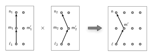
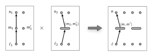
These two experiments can equivalently be viewed as a single experiment performed on a system, , undergoing a sequence of measurements , where each of these measurements is viewed as a composite of the corresponding indexed measurements; for example is viewed as a composite of and . We then say that is a composite system consisting of subsystems and . If, say, measurement yields outcome , and measurement yields , this can be described as measurement yielding an outcome which we symbolize as . The process of composition is illustrated in Fig. 2.
In order that the experiments on and on separately satisfy the experimental conditions stated above, the systems cannot be interacting with one another while the experiments are in progress. If the systems are interacting with one another, then only the two experiments viewed as a whole—as an experiment on —can satisfy these conditions.
II.2 Operationalization of Feynman’s paths and Feynman’s rules
Consider an experimental set-up in which a physical system is subject to successive measurements at successive times , with there possibly being interactions with the system in the intervals between those measurements. Here and subsequently, we assume that the measurements and interactions in any such set-up are selected according to the constraints described above. We summarize the outcomes obtained in a given run of the experiment as the sequence . This is the operational counterpart to a Feynman ‘path’.
We now wish to formalize the idea that set-ups are interrelated in particular ways. In Ref. Goyal et al. (2010), we considered two such relationships. First, the above set-up could be viewed as a series concatenation of two experiments, the first in which measurements and occur at times and , yielding the sequence , and the second in which measurements and occur at times and , yielding . In order to ensure that experimental closure is satisfied in the second experiment, measurement must be atomic. Formally, we express this concatenation as
| (2) |
where is the series combination operator. More generally, the series operator can be used to concatenate two sequences provided their initial and final measurements are atomic, and the final measurement and outcome of the first sequence is the same as the initial measurement and outcome of the second sequence.
Second, one can consider a set-up which is identical to the one above, except that outcomes and of have been coarse-grained, so that one obtains the sequence . Formally, we express the relationship of this sequence to the sequences and as
| (3) |
where is the parallel combination operator. More generally, the parallel operator can combine any two sequences which are identical except for differing in the outcome of a single measurement in the set-up, provided that this measurement is not the initial or final measurement.
Feynman’s Rules in Operational Form
From the above definitions, it follows that the operators and satisfy several symmetry relations, to which we collectively refer to as an experimental logic:
| (4) | ||||
| (5) | ||||
| (6) | ||||
| (7) | ||||
| (8) |
In Ref. Goyal et al. (2010), it is shown that Feynman’s rules are the unique pair-valued representation of this logic consistent with a few additional assumptions. Writing for the complex-valued amplitude that represents sequence , one finds (see Fig. 3):
| (amplitude sum rule) | ||||
| (amplitude product rule) | ||||
| (probability rule) |
These are Feynman’s rules for measurements on individual quantum systems.
III State Formulation of Quantum Theory
In the standard, von Neumann–Dirac formulation of quantum theory, one describes a system by specifying its state at a particular time. Temporal evolution of the system is then represented by a unitary operator, and repeatable measurements made on the system are represented by Hermitian operators. When the states of the subsystems of a composite system are given, the state of the composite system is the tensor product of the subsystem states. In this section, starting from Feynman’s rules and the composite systems rule (derived in Sec. IV), we derive these features with the aid of the no-disturbance postulate.
III.1 No-disturbance postulate
The no-disturbance postulate asserts that a trivial measurement (as defined in Sec. II.1) has no effect on the outcome probabilities of subsequent measurements. For example, in the arrangement shown in Fig. 4, if the trivial measurement , with single outcome , is inserted between measurements and , the probability of outcome given is unaffected.
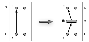
That is,
| (9) |
where in the conditional on the left-hand side indicates that the arrangement containing is the one under consideration.
The no-disturbance postulate can be regarded as capturing the essential departure of quantum physics from the mode of thinking embodied in classical physics. The key point is that, from the classical point of view, if outcome is obtained, one would assert that it is a fact of the matter that the system went either through the field of sensitivity of the detector corresponding to outcome or through that corresponding to , even though neither was, in fact, observed. To see the consequences of this assertion, let us consider the special case where is repeated at time , where is immediately after so that the system undergoes no appreciable temporal evolution in the interim (see Fig. 5).
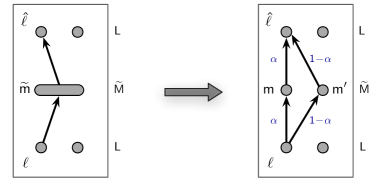
For clarity, we denote outcome of measurement at by . Now, according to the classical assertion,
where we have used the sum and product rules of probability theory in the first two lines, and closure in the third. If we now assume that transition probabilities are symmetric (an assumption that is independently well-supported by experiment), then and . Setting and noting that ,
Since is a repeatable measurement, should be unity. But, for this to be possible, , which cannot hold true unless is or . Therefore, repeatability cannot be preserved by the insertion of except in the special case where one of the outcomes or is certain to occur. That is, on the classical assertion that the occurrence of outcome implies that either outcome or in fact occurs, insertion of will, in general, disturb repeatability of . Conversely, if the no-disturbance postulate is true, one must conclude that the classical assertion is, in general, false.
III.2 Quantum States
We operationally define the mathematical representation of the physical state of a system at any given time as that mathematical object which enables one to compute the outcome probabilities of any measurement (chosen from a given measurement set ) performed upon the system at that time.
First, suppose that a system is prepared at time using measurement , and that measurement is subsequently performed upon it at time . Here, and subsequently, we assume that all measurements belong to the same measurement set, and each have possible outcomes. We label the th outcome of measurement as , where , and the outcomes of other measurements similarly.
Suppose that measurement yields outcome . In order to compute the transition probabilities for every , it suffices to know the amplitude vector whose th component is the amplitude of the sequence . Then, . Since the outcomes of are mutually exclusive and exhaustive, . Insofar as calculating the outcome probabilities of performed at , the object v suffices.
Second, suppose that, at time , instead of , we wish to perform measurement , and to compute its outcome probabilities. To do so, we now make use of the no-disturbance postulate, according to which we can insert the trivial form of measurement , which we denote , prior to measurement , without changing the outcome probabilities of . We insert immediately prior to in order that the system undergo no appreciable temporal evolution between and (see Fig. 6).
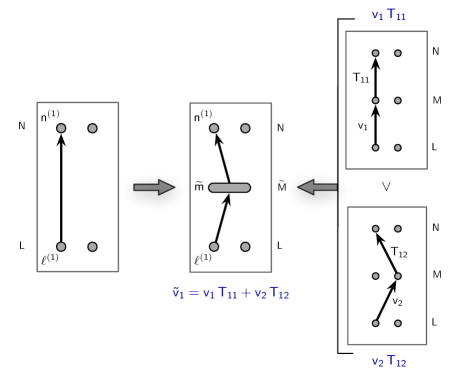
We can now compute the outcome probabilities of in the modified arrangement instead. Now, in this arrangement, the sequence , where , can be decomposed as
| (10) | ||||
| (11) |
Hence, given the amplitudes of the sequences , the amplitude sum and product rules imply that the amplitude of sequence is
| (12) |
where T is a matrix with components . Since the system undergoes no appreciable temporal evolution between measurement and , the matrix T captures precisely the relationship between and . We shall refer to it as the transformation matrix from to . Hence, the transition probability
| (13) |
Using the product rule of probability theory,
| (14) |
and noting that , we obtain
| (15) |
This statement holds for the modified experiment in which occurs. But, by the non-disturbance postulate, it also holds true for the original experiment.
Thus, the object v, which is specified with respect to , not only allows one to compute the outcome probabilities of , but also to compute the outcome probabilities of any other measurement, , provided one is given the transformation matrix, T, from to . Therefore, from the operational point of view stated earlier, v represents the state of the system at time .
III.3 Representation of Measurements
Since the outcomes of are mutually exclusive and exhaustive, Eq. (15) becomes
| (16) |
which implies that . But v can be freely varied by varying the initial measurement , its outcome , and the interaction with the system in the interval . Therefore, the transformation matrix, T, which connects to , is unitary.
To determine the states that can be prepared by measurement , we use the fact that, since is repeatable, if a system is prepared at time using measurement with outcome , the same outcome is obtained when the measurement is immediately repeated. Therefore, using Eq. (15), the state, , that is prepared must be such that
| (17) |
which implies that up to a predictively irrelevant overall phase. In terms of the , one can write , so that Eq. (15) becomes
| (18) |
which is the Born rule with and v specified with respect to . Therefore, measurement can be characterized in terms of the , which form an orthonormal basis of . Alternatively, as is more conventional, we can represent in terms of the Hermitian matrix , where is the value associated with outcome .
In the special case where measurement is the same as , it follows from the repeatability of measurements that . Therefore the transformation matrix that relates to itself has the property that , where the are phases. Now, the states prepared by are predictively relevant only via Eq. (18), whose result is insensitive to the values of the . Therefore, without loss of generality, the can all be set to zero, so that reduces to the identity matrix I. Hence, measurement is represented by a diagonal Hermitian matrix, M.
III.4 Relationship between Representations
Thus far, we have specified the state of the system, v, and the states that are prepared by measurement , with respect to measurement . Suppose that we were instead to represent these states as and with respect to some other measurement . The no-disturbance postulate can then be used to relate the new representation to the old representation by completely coarse-graining measurement and inserting measurement immediately afterwards. If a state is represented by with respect to measurement , and V is the transformation matrix from to , then
| (19) |
so that . Since V is unitary, this can be inverted to give . Similarly , which implies that the Hermitian operator, , that represents with respect to , is given by .
If measurement is represented with respect to by Hermitian matrix with eigenvectors , then the transformation matrix V has components .
III.5 Unitary Representation of Temporal Evolution
Suppose that a system is prepared using measurement at time , and then undergoes measurement at time . Immediately prior to measurement , the system is in state v. Suppose now that measurement is completely coarse-grained, and an additional measurement is performed at time . In this arrangement, the sequence can be decomposed as
| (20) |
The temporal evolution of the system in interval is represented by the amplitudes of the sequences . The amplitude sum and product rules accordingly imply that the amplitude of sequence is
| (21) |
Therefore, the state of the system, , immediately prior to the last measurement is
| (22) |
Now, the initial state v can be arbitrarily varied, but the states v and are normalized. Therefore, U is unitary.
Since temporal evolution from to is represented by U, temporal evolution from to is represented by . Therefore, if we denote the temporal inverse of the sequence as , then
| (23) |
to which we shall refer as the amplitude temporal inversion rule.
III.6 Composite Systems
At time , system is prepared by measurement with outcome , and by measurement with outcome . Suppose that these systems evolve without interacting with one another until time , at which point they are measured, respectively, by and , which respectively have possible outcomes, and , with and . Then the components of the respective states, and , of the systems immediately prior to are given by
| (24) |
Viewed as a single system, , the system is prepared by measurement with outcome , and subsequently undergoes measurement with possible outcomes . With respect to , the components of the state of the system, v, immediately prior to is given by
| (25) |
But, by the composite systems rule, Eq. (44), which we shall derive in Sec. IV,
| (26) |
so that . Hence,
| (27) |
III.7 Summary
In summary, we have derived the following:
-
(i)
If a system is prepared by some measurement at time , then its state at time immediately prior to measurement is given by vector v with respect to reference measurement .
-
(ii)
Measurement is represented by Hermitian operator , where the , also specified with respect to , are the states prepared by . When performed on the system in state v, the probability of the th outcome of is given by
-
(iii)
If the reference measurement is changed to , then the state of the system with respect to is given by , where V is the unitary transformation matrix from to .
-
(iv)
The state v evolves unitarily in the time between measurements.
-
(v)
If the two subsystems of a composite system are in states and , then the composite system is in state .
Collectively, this set of statements is equivalent to von Neumann’s postulates for finite-dimensional quantum systems.
IV Composite Systems
IV.1 Composition Operator and its Symmetries
Suppose that one physical system, denoted , undergoes an experiment involving measurements at successive times , while another system, , undergoes an experiment where the measurements at these same times. The measurements on yield the outcome sequence , while the measurements on yield . As described earlier, in Sec. II.1, one can also describe the situation by saying that measurements and are performed on the composite system , yielding the sequence . We now symbolize the relationship between and by defining a binary operator , the composition operator, which here acts on and to generate the sequence
| (28) |
Generally, the operator combines any two sequences of the same length, each obtained from a different experiments on different physical systems where each measurement in one experiment occurs at the same time as one measurement in the other experiment.
From the definition just given, it follows that is associative. To see this, consider the three sequences , and , obtained from three different experiments satisfying the condition just stated above. We can then combine these to yield the sequence in two different ways, either as or as . Hence,
| (29) |
Similar considerations show that also satisfies the following symmetry relations involving the operators and :
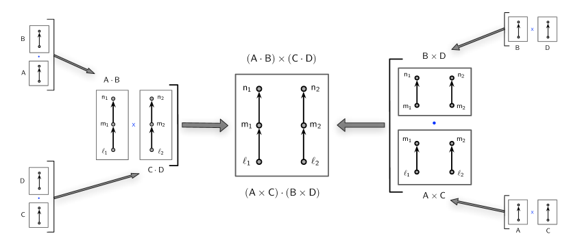
| (30) | ||||
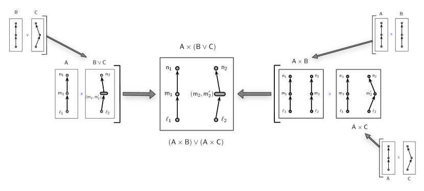
| (31) | ||||
| (32) |
The cross-multiplicativity and left-distributivity properties expressed in Eqs. (30) and (31) are illustrated in Figs. 7 and 8, respectively.
IV.2 Composite Systems Rule
If systems and are noninteracting, we postulate that, in Eq. (28), the amplitude, , of sequence is determined by the amplitudes of the sequences , so that
| (33) |
where is some continuous complex-valued function to be determined. This is the composition postulate, given which Eqs. (29), (30), (31) and (32) respectively imply
| (34) | ||||
| (35) | ||||
| (36) | ||||
| (37) |
We can now solve these for . Due to the cross-multiplicativity equation, Eq. (35),
| (38) |
To determine form of , we use the right-distributivity and cross-multiplicativity equations, Eqs. (37) and (35), respectively, to obtain
Writing , these two equations can be written as a pair of functional equations,
| (40a) | ||||
| (40b) | ||||
whose continuous solutions in the domain are , or (see Appendix A). The zero solution implies for all , and is therefore inadmissible. Therefore,
| (41a) | |||||
| (41b) |
To eliminate the possibility we make use of the associativity equation, Eq. (34), which implies
| (42) |
Now, from the cross-multiplicativity equation, Eq. (35), , which implies since the zero solution for is inadmissible. Therefore, Eq. (42) becomes
| (43) |
But this is incompatible with since . We are therefore left with , which is compatible with Eq. (43). A parallel argument establishes that . Therefore, from Eq. (38),
| (44) |
This is the amplitude rule for distinguishable, noninteracting composite systems. We refer to it as the composite system rule.
V Derivation of Dirac’s amplitude–action rule
Consider a quantum system that is subject to position measurements at a successive times. Suppose that the intervals between these successive times are sufficiently small that the resulting measurement sequence is well approximated by a continuous classical trajectory (or simply ‘path’) of the same system as treated according to the framework of classical physics. Dirac’s amplitude–action rule asserts that the amplitude associated with the measurement sequence is given by , where is the classical action associated with the corresponding classical path. We now derive the form of this rule up to from two elementary properties of the classical action, namely:
-
Additivity. If sequence , then , where is the classical action of the path corresponding to sequence .
-
Inversion. The action associated with sequence is .
Our assumption is that the amplitude, , of sequence , with corresponding classical action is , is given by , where is a continuous, complex-valued function.
The additivity and inversion properties of the classical action induce two functional equations in . First, the amplitude of sequence can be computed in two ways (see Fig. 9),
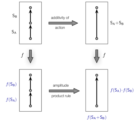
either using the action additivity property,
or using the amplitude product rule,
so that
| (45) |
Second, the amplitude of sequence can be computed either using the amplitude temporal inversion rule, Eq. (23),
or using the action inversion property,
so that
| (46) |
We can solve Eq. (45) by writing , with real, to obtain, for integer ,
| (47) | ||||
| (48) |
The second equation can be transformed via to give
| (49) |
Equations (47) and (49) are two of Cauchy’s standard function equations, with general solutions and , where Aczél (1966). Hence, , and
| (50) |
But Eq. (46) then implies that . Therefore,
| (51) |
where the constant has dimensions of . This is Dirac’s amplitude–action rule up to .
VI Discussion
In this paper, we have shown that it is possible to systematically build Feynman’s rules into a complete formulation of finite-dimensional quantum theory. The key physical ingredient in this process has been the no-disturbance postulate, which expresses the singularly non-classical fact that a trivial measurement does not disturb the outcome probabilities of subsequent measurements on the system. This postulate allows us to introduce the concept of the state of a system in a systematic way, and to prove the unitarity of temporal evolution and the hermiticity of measurement operators. We have also derived the composite system rule and Dirac’s amplitude–action rule, each from a single elementary and natural assumption, by making use of the fact that these assumptions must be consistent with Feynman’s rules.
The work described here, in concert with our earlier derivation of Feynman’s rules, constitutes a complete derivation of the finite-dimensional quantum formalism. The derivation has a number of important implications for our understanding of quantum theory in addition to those mentioned in the Introduction.
First, most other attempts to derive the quantum formalism from physically-motivated postulates (such as Hardy (2001, 2013); Chiribella et al. (2011)) depend upon postulates (such as purifiability Chiribella et al. (2011) or local tomography Hardy (2001, 2013)) that concern the behavior of composite systems in order to derive the quantum formalism for individual systems. This tends to suggest that the behavior of composite systems is in some sense fundamental to the structure of the quantum formalism. However, in the present derivation, there is no such dependency. Instead, we have shown that it is possible to derive the formalism for individual systems without assumptions that overtly concern composite systems, and then to derive the rule for composite systems on the basis of a simple assumption merely by requiring consistency with the formalism for individual systems. Therefore, the present derivation strongly implies that the behavior of composite systems is a secondary feature of quantum theory, not a primary one.
Second, one of the most remarkable features of Feynman’s formulation of quantum theory is the absence of a state concept, and the absence of any distinction between dynamics, on the one hand, and the relationship between measurements, on the other. We have shown here that these features can be recovered, but at the cost of an additional physical postulate which has non-trivial physical content.
Finally, we have shown that Dirac’s amplitude–action rule follows from elementary properties of the classical action via the simple assumption that the amplitude of a sequence is determined by the corresponding action. In contrast with Dirac’s argument, our approach does not depend on the particular form of the classical Lagrangian or on the existence or form of Lagrange’s equations of motion, but only on two elementary properties (additivity, inversion) of the action. Hence, we have shown that Dirac’s rule has a very general validity, and arises as soon as one attempts to establish a quantitative connection between the notion of action in the Lagrangian formulation of classical mechanics, and the notion of amplitude in Feynman’s formulation of quantum theory.
We conclude with two open questions. First, is the no-disturbance postulate related in any way with other informational ideas that have been proposed, such as in Refs. Č. Brukner and Zeilinger (1999); Brukner and Zeilinger (2009); Chiribella et al. (2011)? Second, is there a direct, general path from Dirac’s amplitude–action rule to the unitary form, , of the temporal evolution operator?
Acknowledgements.
This publication was, in part, made possible through the support of a grant from the John Templeton Foundation.References
- Wheeler (1990) J. A. Wheeler, in Foundations of quantum mechanics in the light of new technology: Proceedings of the 3rd international symposium (Physical Society of Japan, Tokyo, 1990).
- Zeilinger (1999) A. Zeilinger, Found. Phys. 29, 631 (1999).
- Fuchs (2002) C. A. Fuchs (2002), quant-ph/0205039.
- Grinbaum (2007) A. Grinbaum, British Journal for the Philosophy of Science 58, 387 (2007).
- Hardy (2001) L. Hardy (2001), eprint quant-ph/0101012.
- Clifton et al. (2003) R. Clifton, J. Bub, and H. Halvorson, Found. Phys. 33, 1561 (2003).
- D’Ariano (2007) G. M. D’Ariano, in Foundations of Probability and Physics, 4, edited by A. Y. K. G. Adenier, C. A. Fuchs (AIP, New York, 2007), p. 79.
- Goyal (2010) P. Goyal, New J. Phys. 12, 023012 (2010), eprint arXiv:0805.2770.
- Reginatto (1998) M. Reginatto, Phys. Rev. A 58, 1775 (1998).
- Goyal et al. (2010) P. Goyal, K. H. Knuth, and J. Skilling, Phys. Rev. A 81, 022109 (2010).
- Chiribella et al. (2011) G. Chiribella, P. Perinotti, and G. M. D’Ariano, Phys. Rev. A 84, 012311 (2011).
- Masanes and Müller (2011) L. Masanes and M. Müller, New J. Phys. 13, 063001 (2011).
- Dakic and Brukner (2011) B. Dakic and C. Brukner, in Deep Beauty: Understanding the Quantum World through Mathematical Innovation, edited by H. Halvorson (Cambridge Univ. Press, 2011), pp. 365–392.
- Barrett (2007) J. Barrett, Phys. Rev. A 75, 032304 (2007), arXiv:quant-ph/0508211v3.
- Pawlowski et al. (2009) M. Pawlowski, T. Paterek, D. Kaszlikowski, V. Scarani, A. Winter, and M. Zukowski, Nature 461, 1101 (2009), arXiv:0905.2292v3.
- Feynman (1948) R. P. Feynman, Rev. Mod. Phys. 20, 367 (1948).
- Feynman and Hibbs (1965) R. P. Feynman and A. R. Hibbs, Quantum Mechanics and Path Integrals (McGraw-Hill, 1965), 1st ed.
- Cox (1946) R. T. Cox, Am. J. Phys. 14, 1 (1946).
- Cox (1961) R. T. Cox, The Algebra of Probable Inference (The Johns Hopkins Press, 1961).
- Goyal and Knuth (2011) P. Goyal and K. H. Knuth, Symmetry 3, 171 (2011).
- Dirac (1930) P. A. M. Dirac, Principles of Quantum Mechanics (Oxford University Press, 1930), 1st ed.
- von Neumann (1955) J. von Neumann, Mathematical Foundations of Quantum Mechanics (Princeton University Press, 1955).
- Johnson and Lapidus (2000) G. Johnson and M. L. Lapidus, The Feynman Integral and Feynman’s operational calculus (Oxford University Press, 2000).
- Fuchs and Peres (1996) C. A. Fuchs and A. Peres, Phys. Rev. A 53, 2038 (1996).
- Pfister and Wehner (2013) C. Pfister and S. Wehner, Nature Comm. 4, 1851 (2013).
- Goyal (2013) P. Goyal, arxiv:1309.0478 (2013).
- Dirac (1933) P. A. M. Dirac, Physikalische Z. der Sowjetunion 3, 64 (1933).
- Feynman (1949) R. P. Feynman, Phys. Rev. 76, 769 (1949).
- Caticha (2000) A. Caticha, Found. Phys. 30, 227 (2000), eprint quant-ph/9810074v2.
- Tikochinsky (1988) Y. Tikochinsky, Phys. Rev. A 37, 3553 (1988).
- Caticha (1998) A. Caticha, Phys. Rev. A 57, 1572 (1998).
- Pearle (1976) P. Pearle, Phys. Rev. D 13, 857 (1976).
- Bialynicki-Birula and Mycielski (1976) I. Bialynicki-Birula and J. Mycielski, Ann. Phys. 100, 62 (1976).
- Shimony (1979) A. Shimony, Phys. Rev. A 20, 394 (1979).
- Weinberg (1989a) S. Weinberg, Phys. Rev. Lett. 62, 485 (1989a).
- Weinberg (1989b) S. Weinberg, Ann. Phys. (N.Y.) 194, 336 (1989b).
- Giddings (1995) S. B. Giddings, hep-th/9508151 (1995).
- Simon et al. (2001) C. Simon, V. Buzek, and N. Gisin, Phys. Rev. Lett. 87, 170405 (2001).
- Ferrero et al. (2004) M. Ferrero, D. Salgado, and J. L. Sánchez-Gómez, Phys. Rev. A 70, 014101 (2004).
- Ferrero et al. (2006) M. Ferrero, D. Salgado, and J. L. Sánchez-Gómez, Phys. Rev. A 73, 034304 (2006).
- Goyal (2008) P. Goyal, Phys. Rev. A 78, 052120 (2008).
- Aczél (1966) J. Aczél, Lectures on Functional Equations and their Application (Academic Press, 1966).
- Hardy (2013) L. Hardy, arxiv:1303.1538 (2013).
- Č. Brukner and Zeilinger (1999) Č. Brukner and A. Zeilinger, Phys. Rev. Lett. 83, 3354 (1999).
- Brukner and Zeilinger (2009) C. Brukner and A. Zeilinger, Found. Phys. 39, 677 (2009).
Appendix A Solution of a pair of functional equations.
We solve Eqs. (40a) and (40b) with the aid of one of Cauchy’s standard functional equations,
| (52) |
where is a real function and . Its continuous solution is with Aczél (1966).