The Picard integral formulation of weighted essentially non-oscillatory schemes
Abstract
High-order temporal discretizations for hyperbolic conservation laws have historically been formulated as either a method of lines (MOL) or a Lax-Wendroff method. In the MOL viewpoint, the partial differential equation is treated as a large system of ordinary differential equations (ODEs), where an ODE tailored time-integrator is applied. In contrast, Lax-Wendroff discretizations immediately convert Taylor series in time to discrete spatial derivatives. In this work, we propose the Picard integral formulation (PIF), which is based on the method of modified fluxes, and is used to derive new Taylor and Runge-Kutta (RK) methods. In particular, we construct a new class of conservative finite difference methods by applying WENO reconstructions to the so-called “time-averaged” fluxes. Our schemes are automatically conservative under any modification of the fluxes, which is attributed to the fact that classical WENO reconstructions conserve mass when coupled with forward Euler time steps. The proposed Lax-Wendroff discretization is constructed by taking Taylor series of the flux function as opposed to Taylor series of the conserved variables. The RK discretization differs from classical MOL formulations because we apply WENO reconstructions to time-averaged fluxes rather than taking linear combinations of spatial derivatives of the flux. In both cases, we only need one projection onto the characteristic variables per time step. The PIF is generic, and lends itself to a multitude of options for further investigation. At present, we present two canonical examples: one based on Taylor, and the other based on the classical RK method. Stability analyses are presented for each method. The proposed schemes are applied to hyperbolic conservation laws in one- and two-dimensions and the results are in good agreement with current state of the art methods.
keywords:
finite difference methods, weighted essentially non-oscillatory, Lax-Wendroff, hyperbolic conservation lawsDepartment of Mathematics, Michigan State University,
East Lansing, Michigan, 48824, USA.
33footnotemark: 3
Department of Electrical and Computer Engineering, Michigan State University,
East Lansing, Michigan, 48824, USA.
44footnotemark: 4 This work was supported in part by AFOSR grants
FA9550-11-1-0281, FA9550-12-1-0343, and FA9550-12-1-0455, NSF grant
DMS-1115709, and MSU
Foundation grant SPG-RG100059.
1 Introduction
We begin our discussion with a 1D system of conservation laws defined by
| (1) |
where is the unknown vector of conserved quantities and is a prescribed flux function. The starting point for this body of work is to perform formal integration of (1) over a single interval , which defines the Picard integral formulation (PIF) of the 1D conservation law as
| (2a) | |||
| where the time-averaged flux is defined as | |||
| (2b) | |||
We use the term Picard to emphasize that we propose solving, at least in spirit, an integral, as opposed to a differential equation in time. Our goal is to construct explicit time-stepping schemes that do not require an iterative procedure. The purpose of defining (2) is that a new class of conservative finite difference methods can be constructed by following the two step process:
-
1.
Approximate the time-averaged fluxes in (2b) with any temporal discretization. We offer the third-order Taylor and the classical fourth-order Runge-Kutta method as two canonical examples.
-
2.
Insert the result into the non-linear finite difference WENO reconstruction procedure, which provides a conservative high-order approximation to the spatial derivative in (2a). We present results that are fifth-order in space.
The combination of these two steps will be called the Picard integral formulation of WENO (PIF-WENO), and we remark that the methods presented here can be extended to arbitrary order in space and time. Some advantages that this formulation provide include:
-
•
Methods that are constructed from this framework are automatically mass conservative, independent upon how the time averaged fluxes are defined.
-
•
A variety of time stepping methods including Runge-Kutta (RK), Taylor, multistep or even multiderivative methods [1] can be constructed from this framework. Currently, we present two methods, one based on a Taylor formulation, and one based on an RK formulation.
-
•
The Picard integral formulation has the capacity to reduce computational complexity, including i) smaller stencils, and ii) a reduction in the number of characteristic variable projections. Both methods presented in this work only require a single projection onto characteristic variables per time step.
The outline of this paper is as follows. In §2 we present background material and in §3, we define two 1D formulations of PIF-WENO, including a third-order Taylor and a fourth-order Runge-Kutta discretization. We continue in §4 with an analysis of the linear stability properties of the proposed methods, and in §5 we extend the results to 2D. Finally, numerical results and conclusions are presented in §6 and §7.
2 Background
Temporal discretizations for hyperbolic conservation laws are oftentimes presented as falling into one of two categories: a method of lines (MOL) or a Taylor/Lax-Wendroff method. In a MOL formulation, one first discretizes in space, and then applies an appropriate time integrator to the problem. Popular high-order methods for hyperbolic conservation laws include finite difference and finite volume weighted essentially non-oscillatory (WENO) methods, discontinuous- and Petrov-Galerkin as well as piecewise parabolic methods (PPMs). The spatial discretizations defines a large system of ordinary differential equations (ODEs), that is then integrated in time by a suitable ODE solver, which is usually an explicit Runge-Kutta method. MOL methods treat spatial and temporal discretizations as separate operations, and therefore miss out on coupling opportunities. In this work, one of the two examples we present includes a new MOL approach that can be derived from the Picard integral formulation. Additionally, we derive Lax-Wendroff type methods from the vantage the Picard integral formulation provides.
The basic procedure in a Lax-Wendroff (Taylor) method is to first discretize in time, and then immediately convert the temporal derivatives to discrete spatial derivatives via the Cauchy-Kowalewski procedure. In doing so, space and time is coupled through the PDE, as opposed to through relying on a system of ODEs. The original Lax-Wendroff method [2] is likely the first numerical method based on this procedure, where second-order accuracy was obtained by including the evaluation of flux Jacobians. The coupling of arbitrarily high order Lax-Wendroff discretizations to finite volume methods was investigated in the 1980’s with the original ENO methods of Harten [3], and starting in the early 2000’s, the so-called Arbitrary DERivative (ADER) methods [4, 5, 6, 7, 8, 9, 10, 11] have grown tremendously in popularity. Recent work also includes coupling the Lax-Wendroff discretization to high-order finite difference WENO [12, 13, 14, 15] and discontinuous Galerkin [16, 17, 18, 19, 20] methods. All high-order Lax-Wendroff discretizations rely on the evaluation of Jacobians, Hessians and higher derivatives that inevitably show up for all high-order single-step methods. The finite difference WENO methods that fall into this category typically compute the first derivative with a single non-linear WENO reconstruction, and then use (centered) finite differences to compute higher derivatives. The finite volume flavored methods including the discontinuous Galerkin and ADER methods [21, 20] rely on high-order solutions to generalized Riemann problems [9]. The common thread in these methods is that the time dependence is immediately removed in the process of converting temporal to spatial derivatives. When compared with Runge-Kutta methods, there are no degrees of freedom to work with because each coefficient in a Taylor series expansion is unique.
The purpose of this work is to define a new class of non-linear methods for hyperbolic conservation laws based on the Picard integral formulation, to which many existing methods can be derived. For example, many finite volume formulations including the original Godunov scheme, “high-order” variations of the scheme [22, 23, 24, 3, 25, 26], Harten’s original ENO method [3], and modern ADER methods [7, 8, 10, 11] work with time-averaged fluxes approximated through Taylor series. In these formulations, one takes the further step of integrating (2a) over a control element and then applying the divergence theorem. This defines an evolution equation for the unknown cell averages, which is based on integrating (2b) over the boundaries of each control element. The differences in the methods primarily come from the choice in discretization of the time-averaged fluxes, as well as how each Riemann problem is solved. For example, in 1959 Godunov discretized the time-average fluxes with constants; his insight was to leverage exact Riemann solvers for piecewise constant functions. In 1979 Van Leer [22] introduced piecewise linear approximations to the solution, and therefore was able to define a second-order version of Godunov’s method. A decade later, Harten, Engquist, Osher and Chakravarthy [3] defined an essentially non-oscillatory method that used piecewise polynomial reconstructions of the solution from cell averages, and therefore were able to extend Godunov’s method to arbitrary order. In their seminal paper, time was discretized via the Cauchy-Kowalewski/Lax-Wendroff procedure, which resulted in a single-stage, single-step method [3]. A further decade later, the now classical ADER formulation was defined [4], where additional Arbitrary DERivative Riemann problems were introduced in order to define an arbitrary order, single-step finite volume method. Our focus is not on finite volume methods, nor their discontinuous Galerkin cousins, but on conservative finite difference methods.
The vantage the Picard integral formulation provides allows one to produce a variety of conservative finite difference schemes. To the authors’ knowledge, the first conservative finite difference scheme that can be cast under this light is the 1D semi-Lagrangian solver created by J-M Qiu and Shu in 2011 [27]. There, the authors solve with semi-Lagrangian technology, which converts temporal integrals into spatial integrals. Results are extended to 2D incompressible flows by applying operator splitting techniques. In order to maintain mass conservation, they make use of a time-averaged version of the usual discrete implicit flux function, which is not explicitly stated in their work. We elaborate and extend this idea in §3.1.
Our contribution is the development of time-averaged fluxes for conservative finite difference methods, which include non-linear scalar, and systems of equations for single and multidimensional systems of hyperbolic conservation laws. Furthermore, we introduce an entirely new interpretation of time-averaged fluxes that can be applied to a large class of Runge-Kutta methods. Both the Taylor and Runge-Kutta interpretation only require a single projection onto characterstic variables per time step. We make use of time-averaged discrete implicit flux functions in order to retain mass conservation. We refer the reader to the references for details on the essentially non-oscillatory method [3, 28, 29], as well as the weighted essentially non-oscillatory method [30, 31, 32, 33]. The Picard integral formulation is agnostic towards the choice of time discretization, and therefore we begin by presenting the conservative finite difference reconstruction procedure based upon time-averaged fluxes. Two examples of time discretizations are presented in §§3.3-3.4, a stability analysis is presented in §4, and the extension to 2D is presented in §5.
3 The 1D Picard integral formulation
3.1 1D conservative finite differences with time-averaged fluxes
Consider a uniform grid of equidistant points in :
| (3) |
In a finite difference method, one enforces some approximation to (1) to hold on a finite set of points , and seeks point value approximations to hold at discrete time levels .
The classical conservative finite difference WENO method implicitly defines a function , whose sliding average111The term ‘sliding average’ was borrowed from the high-order finite volume methods of Harten and collaborators [3] before being imported to conservative finite difference methods [28, 29]. agrees with via
| (4) |
We consider a time-averaged version of this implicit function, defined by
| (5) |
After integrating (4) in time, we see
| (6) |
We remark that (6) is similar to the usual averaging property found in finite difference methods, but the primary departure is that we have chosen to integrate both the flux and the primitive of the flux function in time, which differs from what is typically done in a finite difference WENO method, where the reconstruction procedure is carried out at discrete “frozen in time” levels. We now point out two important properties concerning the implicitly defined function, which are in common with any classical MOL formulation:
-
•
High-order reconstruction algorithms can produce high-order interface values by identifying cell averages as known point values: , where , and therefore need never be computed.
- •
Once (7) has been defined, the complete finite difference PIF-WENO method is given by inserting the result into (2), which results in a single-step update
| (8) |
where . Before providing the description of how the are constructed, we point out a single remark followed by an important theorem.
Remark 1.
In the case where the time-averaged fluxes are approximated as constants through , the PIF-WENO formulation reduces to a single Euler step of a classical WENO method.
Theorem 1.
No matter how the quantities are approximated, on an infinite or periodic domain, the update defined by (8) satisfies the conservation property
| (9) |
Proof.
Sum equation (8) over all . ∎
This theorem is a consequence of the deliberate choice of the order of operations used to carry out (2). Its significance means that the time-averaged fluxes can be discretized in any manner without violating mass conservation. Under the assumption that the have been approximated at each grid point, we are now ready to describe the finite difference WENO procedure for systems. A Taylor discretization will be presented in §3.3, and a Runge-Kutta discretization will be presented in §3.4.
3.2 The finite difference WENO method with time-averaged fluxes
- 1.
-
2.
Compute the left and right eigenvalue decomposition of at the half-grid points
Compute the fastest (scalar) local wave speed
Our definition of is nominally different than other definitions that have been used for local wave speeds in finite difference WENO methods [35, 36]. For stability, we follow the common practice of increasing this speed by exactly 10% and define , which helps to guarantee that the approximate wave speeds encompass the exact solution to a Riemann problem.
-
3.
For each , determine the weighted ENO stencil surrounding . In fifth-order WENO, the full stencil is given by . Project each and each time-averaged flux value onto the characteristic variables using the linear mapping
(11a) (11b) Apply a (local) Lax-Friedrichs flux splitting to (11)
(12) As an alternative, one could use a global wave speed.
-
4.
Perform a WENO reconstruction on each of the characteristic variables separately. Use the stencil that uses an extra point on the upwind direction for defining :
See Appendix A for a description of this function. Define .
-
5.
Using the same projection matrix, , project characteristic variables back onto the conserved variables
To summarize, given any modified flux function , we compute with WENO reconstructions applied to flux-split characteristic decompositions. The result is inserted into (8) to update the solution. This procedure can be carried out independent of the choice of how the temporal integrals are discretized. As pointed out in Remark 1, this formulation reduces to classical WENO with forward Euler time-discretization if the time-averaged fluxes are approximated with constants. We present two methods of increasing the temporal accuracy: a Taylor and a Runge-Kutta example.
3.3 A Taylor series discretization of the 1D Picard integral formulation
Consider a Taylor expansion of centered at , and define an approximation to the time-averaged flux as
| (13) |
These temporal derivatives can be computed via the Cauchy-Kowalewski procedure. For example, in 1D the first two derivatives are
| (14) | ||||
| (15) | ||||
where is the Jacobian matrix of , and is the Hessian tensor222Given two vectors , the Hessian product is defined as the vector whose -component is .. Further derivatives produce tensors that grow exponentially in size. We compute point values using the following finite difference formulas on a single 5-point stencil:
| (16a) | ||||
| (16b) | ||||
Higher derivatives can be included using the same stencil. They will start to lose single orders of accuracy, but because those derivatives are multiplied by increasing powers of the overall order of accuracy is retained. This is consistent with previous results in the literature [12, 16, 15, 37]. This defines a single value for each , and therefore any stencil can be used without violating mass conservation.
It bears notice to compare the present Taylor discretization with similar finite difference Lax-Wendroff discretizations for the same problem. For example, similar to Jiang, Shu and Zhang’s recent work [15], we have taken care to expand the second spatial derivative involving because this allows us to compute the first, second and possibly high-order derivatives on the same stencil by differentiating the same interpolating polynomial. Without expansion, one could compose a first-derivative finite difference stencil with itself, but that increases the size of the computational stencil. Indeed, in Qiu and Shu’s earlier work [12], the authors perform compositions of finite differences that creates a rather large effective stencil. Moreover, their method requires the use of central finite differences in order to retain mass conservation, whereas our scheme could have used any approximation to the time-averaged flux. The primary difference that the Taylor discretization of the Picard integral formulation carries is its generality.
In §5 we follow the direct extension of this method to the two-dimensional case, but first we present an alternative MOL type of method that can be derived from the Picard integral formulation.
3.4 A Runge-Kutta discretization of the 1D Picard integral formulation
As an alternative to the single-stage, single-step multiderivative Taylor method from the previous section, one could pursue a high-order collocation type of method to discretize the time-averaged fluxes. For example, an application of the fourth-order Simpson’s rule to (2b) would define
| (17) |
where . Given the prohibitively expensive cost of this implicit scheme, we would prefer an explicit reinterpretation of (17). For example, it is well known that when the classical four-stage, fourth-order Runge-Kutta method (RK4) is applied to an ODE whose right hand side depends on time only, then Simpson’s rule and RK4 are identical. Therefore, we will interpret the final step in a Runge-Kutta scheme as the approximation to an integral, which allows us to derive a new class of Runge-Kutta type methods from the Picard integral formulation.
We begin our discussion with a focus on the temporal discretization. For example, the RK4 method applied to (1) defines the first stage as . Further stages are given by
| (18a) | |||
| (18b) | |||
| (18c) | |||
and the final update is given by
| (19) |
Equations (18) and (19) define the classical MOL temporal discretization of finite difference, finite volume or discontinuous Galerkin methods, where each continuous spatial differentiation constitutes a linear (in some cases of DG), or non-linear (in the case of FD or FV-WENO) discrete differentiation operator. In any case, the Picard integral formulation will allow us to view (19) from a new angle.
For example, in place of updating our solution with (19), we define
| (20) |
which is a high-order approximation to the exact time-averaged flux. After inserting (20) into (2a), we apply the conservative finite difference WENO method as described in §3.2 to the result, which updates our solution after each stage value has been computed. It remains to define how each stage value is computed.
If each stage value in (18), were computed with the full FD-WENO procedure, then the method described so far would be computationally equivalent to applying a standard MOL discretization. However, in the Picard integral formulation, we have the leeway to modify the fluxes and therefore can reduce the computational cost of the method. For example, we find that for each stage in Eqn. (18), there is no need to project onto the characteristic variables in Step 3 of §3.2, and therefore Steps 1,2 and 5 of §3.2 can be skipped. The end result is that we can construct a method that requires only one characteristic projection per time step in place of a total of four characteristic projections. This is a large savings for systems of equations, given that matrices for each flux interface as well as the multiplication of each of these matrices over the footprint of each interface value can be avoided. Additionally, one could consider replacing the non-linear fifth-order reconstruction procedure in Step 4 with other methods. However, after numerical experimentation, we have found that further limiting in the form of a non-linear reconstruction is necessary in order to obtain non-oscillatory behavior for methods with sufficiently large time steps.
We repeat that many variations of the methods presented thus far can be derived from the Picard integral formulation. We simply advocate the use of constructing discretizations for time-averaged fluxes in place of the usual “frozen-in-time” approximations. Extensions to 2D are straightforward, and will be presented in §5.
4 Linear stability analysis
Linear stability analysis for finite difference WENO methods is difficult given that the WENO reconstruction procedure is a non-linear operator. In this section, we follow the common convention of assuming the so-called linear weights [38, 39], which are valid in smooth regions. Additionally, we assume the ideal wave speed case where we do not increase the value of in Step 2 of §3.2.
A typical stability analysis usually relies on the two step procedure: i) determine the eigen-spectrum of the spatial discretization operator, followed by ii) consider the test problem and verify that the region of absolute stability for the ODE solver contains each eigenvalue from the spectrum of the spatial discretization operator. At first glance, it is not readily obvious that the RK formulations derived from the Picard integral follow this same recipe. However, it will be shown in this section that they have identical stability regions to their MOL counterparts, under the assumption of linear reconstruction weights. However, the Taylor formulations derived from the Picard integral formulation carry an added difficulty which will be addressed at the end of this section.
4.1 Linear stability analysis for the Runge-Kutta discretization
In this section, we will show that Runge-Kutta methods constructed from the Picard integral formulation have identical stability regions to their classical MOL counterparts. Without much added difficulty, we show the generic case in place of focusing on fourth-order Runge-Kutta, and in turn, this defines the extension of the method already presented in §3.4.
To begin, consider scalar advection,
| (21) |
whose flux function is defined as , with being a constant. The application of a Runge-Kutta method in a classical MOL formulation produces a final update of the form
| (22) |
where is the current approximation to the vector of conserved variables, is the discrete derivative of the flux function, and are the coefficients from the Butcher tableau of the method. The RK discretization of the PIF formulation computes stage values that are identical to those computed from the MOL discretization. This is because the RK discretization of PIF neglects characteristic projections, and (21) is a scalar problem. Therefore, the only possible difference would be the final update, which we now show is identical.
The proposed RK methods derived from the Picard integral formulation update the solution with
| (23) |
in place of (22). The derivative in (23) would normally be interpreted as a non-linear operator, but under the assumption of linear weights, we may proceed further with the analysis. Now, consider the linear discrete spatial discretization operator that approximates the derivative of the function. After inserting into (23), the discrete update for the proposed class of methods becomes
| (24) |
This is identical to (22) after inserting , and therefore the two schemes have identical stability limits. The primary difference is that the second equality in (24) is only valid under the assumption of linear weights. The non-linear WENO reconstruction procedure that computes the derivatives of the solution will make the methods different in the presence of shocks. A complete analysis of the non-linear method is beyond the scope of the present work, but would follow according to recent results [38, 39], which first requires an analysis of the linear weights.
4.2 Linear stability analysis for the Taylor discretization
The Taylor series methods that discretize time with the Lax-Wendroff procedure require a deeper analysis. To see the added difficulty, recall that the semi-discrete version of (25) is given by
| (25) |
If a third-order Taylor method were to be directly applied to the semi-discrete ODE in (25), then the update would look like
| (26) |
However, when performing the Lax-Wendroff procedure, higher derivatives do not come from (25), but from approximating higher derivatives of the PDE. Moreover, the Taylor discretization of the Picard integral formation operates on the fluxes, and not on the conserved variables. To see the difference, we factor out a single term from (26), and rewrite it as
| (27a) | ||||
| (27b) | ||||
The outermost derivative is approximated with the difference operator , but the interior derivatives are approximated with Equation (16) as opposed to composing the conservative reconstruction procedure with itself multiple times. The purpose of doing this was to retain a compact stencil. As is common with all Lax-Wendroff type of methods, we cannot simply study the eigen-spectrum of (25) in our analysis, and we therefore turn to a fully discrete von Neumann analysis.
To begin, we assume the solution to Eqn. 21 has the form , where , , is the grid spacing, and is a a single wave number [40]. If we insert this into our Taylor method, a single update can be written as , where the amplification factor is given by
| (28) |
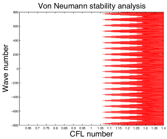
and the CFL number is defined as . Details on deriving the amplification factor were computed using the open-source symbolic toolkit SymPy and have been omitted for brevity. The method is stable for a given time step and grid spacing provided that for all wave numbers .
Note that the amplification factor is a polynomial in and . The degree of represents the temporal order, and the degree of represents the footprint of the stencil. Indeed, the fourth-order Taylor version of our method would contain a term involving , and assuming we restrict our attention to the identical stencil used to compute each derivative in Eqn. 16, the polynomial multiplying will have terms ranging from down to .
In light of attempting to find the roots of , in Fig. 1 we plot the absolute value of as a function of the CFL number, and wave number.
5 The 2D Picard integral formulation
A 2D conservation law is given by
| (29) |
Similar to the 1D case, we define the 2D Picard integral formulation as
| (30a) | |||
| where the time-averaged fluxes are defined by | |||
| (30b) | |||
We again propose an application of the finite difference WENO method to the time-averaged fluxes in place of the usual “frozen in time” approximation to the physical fluxes. We repeat that many options for discretizing (30b) exist. We begin with a description of how the 2D finite difference WENO method can be applied under the assumption that one such time-averaged approximation has been made.
5.1 2D conservative finite differences with time-averaged fluxes
We start with a discretization of the domain given by
| (31a) | ||||||
| (31b) | ||||||
The finite difference method seeks pointwise approximations to hold at each of these grid points.
In the hyperbolic 2D case, one has two eigen-decompositions for and , to which the procedure described in §3.1 is applied on a dimension by dimension fashion. In place of the instantaneous point-wise values such as and , we propose using suitable approximations of and to the time-averaged fluxes in (30b). That is, we will define an update of the form
| (32) |
where the differences in and approximate discrete derivatives of and , respectively, via the non-linear WENO reconstruction procedure. Similar to Remark 1, we point out the following special case.
Remark 2.
If and , then (32) is identical to a single Euler step of a classical RK-WENO method. It is the inclusion of higher-order terms in the approximation of the time-averaged fluxes that increases the temporal order of accuracy.
Remark 3.
This method is automatically mass conservative given any time-averaged flux. This follows from the 2D extension of Theorm 1.
We repeat that many options exist for constructing the time-averaged fluxes. At present, we offer Taylor methods and Runge-Kutta methods; additional methods are currently under investigation, and will be presented in a follow up work.
5.2 A Taylor series discretization of the 2D Picard integral formulation
We define Taylor discretizations of the time-averaged fluxes with
| (33a) | |||
| (33b) | |||
Similar to the 1D case, analytical temporal derivatives can be computed via the Cauchy-Kowalewski procedure. Derivatives of the first component in the flux function are given by
| (34) | ||||
| (35) |
where an expansion of the final time derivative is given by
| (36) | ||||
Note that third-order accuracy requires an approximation to the mixed derivatives and . Similarly, the temporal derivatives of can be expressed with
| (37) | ||||
| (38) |
We compute the first- and second-derivatives of and on a dimension by dimension fashion, with the coefficients prescribed by equations (16a)-(16b). The singular departure from the 1D case is that we require an approximation for the cross-derivative terms. These could be computed through a composition of finite differences or inclusion of off diagonal terms in the stencil. In order to retain a compact stencil, we choose the latter approach, to which we apply the finite difference formula
| (39) |
Given that they are eventually multiplied by a factor of , we only compute these to second-order. In the past, these cross-derivatives have been computed by applying a single finite difference stencil multiple times [12], which results in a large effective stencil.
The complete scheme is given by inserting
| (40) |
into the conservative finite difference reconstruction procedure.
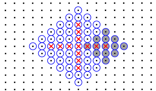
This current proposal provides an additional departure from previous finite difference Lax-Wendroff works [12, 15], because we use a single inexpensive stencil to compute the time-averaged fluxes everywhere in the domain, and then follow that with a single WENO reconstruction. Moreover, from the 2D extension of Theorem 1, further limiting in the form of non-conservative WENO differentiation is an option for us to compute higher derivatives of the flux function. The overall effective stencil is presented in Fig. 2, and is much smaller than Qiu and Shu’s original method [12], and similar in size but different in shape to Jiang Shu and Zhang’s recent proposal [15]. The shaded cells indicate the size of the stencil used in the first pass, and the red ‘X’ terms indicate the stencil required for the WENO reconstruction. An implementation that uses a single loop over the domain would require access to every circled element to update the solution at one point.
5.2.1 A brief note on implementing the Taylor method
One simple implementation of the proposed Taylor method that requires minimal modification to existing codes uses two loops over the computational domain:
-
1.
Compute the time-averaged fluxes and with finite differences on the conserved variables. The benefit is that no characteristic projections or non-linear reconstructions are necessary. However, Taylor methods in particular require additional algebraic operations and therefore the computational expense comes from the need to evaluate high-derivatives using Jacobians and Hessians that increase in size.
-
2.
Use the time-averaged fluxes and to perform the usual WENO reconstruction with an existing sub-routine. The cost of this step is equivalent to that of a single WENO reconstruction.
We remark that the storage required for this particular implementation of the Taylor method is competitive with low-storage Runge-Kutta methods [41, 42, 43, 44]. In particular, any three-stage Runge-Kutta method applied to the classical MOL formulation will require a total of three WENO reconstructions, whereas we make a first pass with an inexpensive linear finite difference stencil, and then follow that up with a single WENO reconstruction. In addition, because it is a single-step Taylor method, this method is amenable to adding adaptive mesh refinement, which is a non-trivial task for multistage methods.
5.3 A Runge-Kutta discretization of the 2D Picard integral formulation
The extension of the RK formulated PIF-WENO method to 2D is straightforward. For example, the 2D analogue of Eqn. (20) from §3.4 is to define the time-averaged fluxes as
| (41a) | ||||
| (41b) | ||||
which are high-order approximations to the exact time-integrated flux functions, and in (30b). Again, the values , for are computed from the RK stages, which do not require characteristic projections. Identical to the 1D case, the complete WENO reconstruction procedure is only applied to the final stage. Similar to classical finite difference WENO methods, this reconstruction procedure is applied in a dimension by dimension fashion, which requires projections onto the characteristic variables. The difference here is that we operate on time-averaged fluxes, and , as opposed to “frozen in time” flux values.
When comparing the two methods presented in this work, the primary difference the RK method has from the Taylor method is that the integral for the time-averaged flux is computed through a collocation type of procedure, which requires computing approximate stage value for the flux functions. Again, we find that it is not necessary to perform characteristic projections of the fluxes and conserved variables for each intermediate stage value.
6 Numerical Results
6.1 1D Burger’s equation
We begin our numerical results section with a convergence study on smooth solutions to inviscid Burger’s equation:
| (42) |
We take the computational domain to be and apply periodic boundary conditions. The initial conditions are prescribed by . For our convergence study, we choose a final time of before any shocks develop.
Exact solutions to this problem can be found implicitly by applying the method of characteristics [40]. With initial conditions defined by , the exact solution is
| (43) |
where is an implicit solution to . To construct exact solutions, we solve (43) at each grid point using Newton iteration with a tolerance of .
In 1D, we use relative errors with the norm defined by point-wise values
| (44) |
and we define the CFL number as the dimensionless quantity
| (45) |
A convergence study for the Taylor discretization of PIF-WENO is presented in Table 1, and a convergence study for the RK discretization of PIF-WENO is presented in Table 2.
In Jiang, Shu and Zhang [15], the authors compare results of their finite difference WENO method in a side-by-side table against the older Qiu and Shu method [12]. However, the new simulations use a smaller CFL number of as opposed to the value of reported in the earlier paper. For completeness, in Table 1 we present results of our method for both CFL numbers. We make two brief observations:
-
•
Large CFL numbers bring out the temporal error faster, and therefore high-order in time is likely more important to reduce error if a user wishes to take large time steps.
-
•
For coarse grids, the difference in errors between the two CFL numbers is quite small, indicating that in this case, high-order spatial accuracy is more important than a high temporal order of accuracy.
Similar to past investigations, for coarse meshes the spatial error dominates, and therefore the algebraic order is higher than expected. This practice is commonplace in the WENO literature, where authors often use lower order time-integrators such as SSP-RK3 [28, 45], and present results indicating fifth or higher order convergence rates. We observe this with the Runge-Kutta discretization presented in Table 2. In this work, we refine our mesh until the temporal error is observable.
| Mesh | Error () | Order | Error () | Order |
|---|---|---|---|---|
| — | — | |||
| Mesh | Error () | Order | Error () | Order |
|---|---|---|---|---|
| — | — | |||
6.2 The 1D Euler equations
The Euler equations describe the evolution of density , momentum and energy of an ideal gas:
| (46) |
where is the pressure. The energy is related to the primitive variables , and by , and is the ratio of specific heats. For all of our simulations, we take .
6.2.1 The 1D Euler equations: a Riemann problem
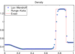
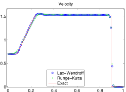
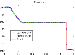
We present a difficult test case. This is commonly referred to as the Lax shock tube, however, the initial conditions are those defined by Harten [46, 3]:
| (47) |
We select for the final time of our simulation [12], and we use a computational domain of with outflow boundary conditions. Results for our method applied to this problem are presented in Fig. 3.
6.2.2 The 1D Euler equations: shock entropy
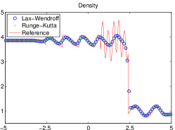
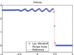
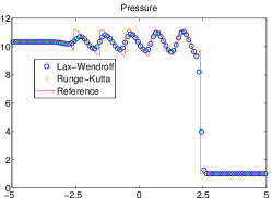
Our final 1D test case is another problem that is popular in the literature [29]. The initial conditions are
with a computational domain of . The final time for this simulation is . With , this is a pure Mach 3 shock moving to the right. We follow the common practice of setting . Results for the new method are presented in Fig. 4.
6.3 The 2D Euler equations
In 2D the Euler equations become
| (48) |
where is the -component of velocity, and is the -component of velocity. Now, the total energy relies on both components of the velocity: .
6.3.1 The 2D Euler equations: a smooth solution
We present convergence results for a smooth solution proposed elsewhere in the literature [12, 16]. The initial conditions are prescribed by
and we compute the solution on a periodic domain . The exact solution has an evolving density, , and constant velocities and pressure . A convergence study for this 2D problem is presented in Table 3. In 2D, we define the relative error as
| (49) |
and the CFL number is defined by
| (50) |
| Mesh | PIF-Taylor | Order | SSP-RK3 | Order | PIF-RK4 | Order |
|---|---|---|---|---|---|---|
| — | — | — | ||||
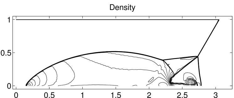
6.3.2 The 2D Euler equations: double mach reflection
We now present results for the so-called double mach reflection originally proposed by Woodward and Colella [47] that was intended to serve as a test problem to compare numerical methods. This problem has since become ubiquitous in the literature [31, 35, 48, 49, 7]. The initial conditions describe a Mach-10 shock incident upon a single wedge (c.f. Fig. in [48]). The computational domain is tilted, so that the wedge is positioned along the bottom of the grid. The shock forms an oblique angle with the mesh, where it starts at the front of the wedge located at , and continues up to the top of the computational domain located at . The initial conditions describe two constant values, one to the left and one to right of the shock as
| (51) |
Reflective boundary conditions are applied along the bottom edge when , and the exact pre- and post-shock values are padded everywhere else. In order to pad the correct boundary conditions along the top, we require the exact location of the shock at time along the line , which is given by . Results for this problem are presented in Fig. 5. Given that a consensus concerning what contour lines to plot has not been reached, we plot the 30 equally spaced contours from to , as reported in one of the many simulations presented by the original authors [47].
7 Conclusions
We have formulated and presented results for the Picard integral formulation of the finite difference WENO method. The new formulation allows us to step back from the classical formulations and include the spatial discretization as part of the temporal discretizations. We have demonstrated how Taylor and Runge-Kutta methods can be developed from this new vantage, and have introduced results for the proposed formulation in one- and two-dimensions, that indicate the new methods compete with current state of the art technology. Future work will include investigating positivity-preserving limiters for finite difference methods, as well as other temporal discretizations of the time-averaged fluxes including multiderivative and alternative flux modifications.
Acknowledgments We would like to thank the anonymous reviewers for their thoughtful comments and encouragement to include more extensive results. In addition, we would like to thank Gwendolyn Miller Seal for creating one of the figures used in this manuscript, and Nathan Collins for aid in manipulating the symbolic expressions used to generate source code for the simulations. Finally, we would like to thank Scott Moe for providing feedback on the revised manuscript.
Appendix A WENO reconstruction
For completeness, we present the coefficients required to reproduce the results in this paper. We restrict our attention to the fifth-order case, which uses a five point stencil shifted to the left or right of each cell interface:
Here, the known values are the cell averages
for some scalar function . The purpose of having a “” and “” value is to define upwind stencils that are numerically stable [40]. We define coefficients for the function , and by symmetry, we define
| (52) |
Three sub-stencils define quadratic polynomials that offer competing third-order accurate values for :
| (53a) | ||||
| (53b) | ||||
| (53c) | ||||
A linear combination of (53a)-(53c) yields a fifth-order accurate approximation with linear weights . The WENO procedure replaces the linear weights with nonlinear weights based on the smoothness indicators . In fifth-order WENO, the indicators are
| (54) |
The Jiang and Shu weights [31] are defined by
| (55) |
We use the power parameter and regularization parameter for all of our simulations. With these definitions in place, the final reconstructed value is defined as
| (56) |
References
- [1] E. Hairer and G. Wanner, “Multistep-multistage-multiderivative methods of ordinary differential equations,” Computing (Arch. Elektron. Rechnen), vol. 11, no. 3, pp. 287–303, 1973.
- [2] P. Lax and B. Wendroff, “Systems of conservation laws,” Comm. Pure Appl. Math., vol. 13, pp. 217–237, 1960.
- [3] A. Harten, B. Engquist, S. Osher, and S. R. Chakravarthy, “Uniformly high-order accurate essentially nonoscillatory schemes. III,” J. Comput. Phys., vol. 71, no. 2, pp. 231–303, 1987.
- [4] E. F. Toro and V. A. Titarev, “ADER: Arbitrary high order Godunov approach,” Journal of Scientific Computing, vol. 17, no. 1-4, pp. 609–618, 2002.
- [5] E. F. Toro and V. A. Titarev, “Solution of the generalized Riemann problem for advection-reaction equations,” R. Soc. Lond. Proc. Ser. A Math. Phys. Eng. Sci., vol. 458, no. 2018, pp. 271–281, 2002.
- [6] E. F. Toro and V. A. Titarev, “TVD fluxes for the high-order ADER schemes,” J. Sci. Comput., vol. 24, no. 3, pp. 285–309, 2005.
- [7] V. A. Titarev and E. F. Toro, “ADER schemes for three-dimensional non-linear hyperbolic systems,” J. Comput. Phys., vol. 204, no. 2, pp. 715–736, 2005.
- [8] M. Dumbser and M. Käser, “Arbitrary high order non-oscillatory finite volume schemes on unstructured meshes for linear hyperbolic systems,” J. Comput. Phys., vol. 221, no. 2, pp. 693–723, 2007.
- [9] E. F. Toro and V. A. Titarev, “Derivative Riemann solvers for systems of conservation laws and ADER methods,” J. Comput. Phys., vol. 212, no. 1, pp. 150–165, 2006.
- [10] M. R. Norman and H. Finkel, “Multi-moment ADER-Taylor methods for systems of conservation laws with source terms in one dimension,” J. Comput. Phys., vol. 231, no. 20, pp. 6622–6642, 2012.
- [11] D. S. Balsara, C. Meyer, M. Dumbser, H. Du, and Z. Xu, “Efficient implementation of ADER schemes for Euler and magnetohydrodynamical flows on structured meshes—speed comparisons with Runge-Kutta methods,” J. Comput. Phys., vol. 235, pp. 934–969, 2013.
- [12] J. Qiu and C.-W. Shu, “Finite difference WENO schemes with Lax-Wendroff-type time discretizations,” SIAM J. Sci. Comput., vol. 24, no. 6, pp. 2185–2198, 2003.
- [13] W. Liu, J. Cheng, and C.-W. Shu, “High order conservative Lagrangian schemes with Lax-Wendroff type time discretization for the compressible Euler equations,” J. Comput. Phys., vol. 228, no. 23, pp. 8872–8891, 2009.
- [14] C. Lu and J. Qiu, “Simulations of shallow water equations with finite difference Lax-Wendroff weighted essentially non-oscillatory schemes,” J. Sci. Comput., vol. 47, no. 3, pp. 281–302, 2011.
- [15] Y. Jiang, C.-W. Shu, and M. Zhang, “An alternative formulation of finite difference weighted ENO schemes with Lax-Wendroff time discretization for conservation laws,” SIAM J. Sci. Comput., vol. 35, no. 2, pp. A1137–A1160, 2013.
- [16] J. Qiu, M. Dumbser, and C.-W. Shu, “The discontinuous Galerkin method with Lax-Wendroff type time discretizations,” Comput. Methods Appl. Mech. Eng., vol. 194, no. 42-44, pp. 4528–4543, 2005.
- [17] M. Dumbser and C.-D. Munz, “Building blocks for arbitrary high order discontinuous Galerkin schemes,” J. Sci. Comput., vol. 27, no. 1-3, pp. 215–230, 2006.
- [18] A. Taube, M. Dumbser, D. S. Balsara, and C.-D. Munz, “Arbitrary high-order discontinuous Galerkin schemes for the magnetohydrodynamic equations,” J. Sci. Comput., vol. 30, no. 3, pp. 441–464, 2007.
- [19] J. Qiu, “A numerical comparison of the Lax-Wendroff discontinuous Galerkin method based on different numerical fluxes,” J. Sci. Comput., vol. 30, no. 3, pp. 345–367, 2007.
- [20] G. Gassner, M. Dumbser, F. Hindenlang, and C.-D. Munz, “Explicit one-step time discretizations for discontinuous Galerkin and finite volume schemes based on local predictors,” J. Comput. Phys., vol. 230, no. 11, pp. 4232–4247, 2011.
- [21] M. Dumbser, D. S. Balsara, E. F. Toro, and C.-D. Munz, “A unified framework for the construction of one-step finite volume and discontinuous Galerkin schemes on unstructured meshes,” J. Comput. Phys., vol. 227, no. 18, pp. 8209–8253, 2008.
- [22] B. van Leer, “Towards the ultimate conservative difference scheme. V. A second-order sequel to Godunov’s method,” J. Comput. Phys., vol. 32, no. 1, pp. 101–136, 1979.
- [23] A. Harten, “On a class of high resolution total-variation-stable finite-difference schemes,” SIAM J. Numer. Anal., vol. 21, no. 1, pp. 1–23, 1984.
- [24] A. Rodionov, “Methods of increasing the accuracy in Godunov’s scheme,” USSR Computational Mathematics and Mathematical Physics, vol. 27, no. 6, pp. 164 – 169, 1987.
- [25] J. B. Bell, P. Colella, and J. A. Trangenstein, “Higher order Godunov methods for general systems of hyperbolic conservation laws,” J. Comput. Phys., vol. 82, no. 2, pp. 362–397, 1989.
- [26] I. Men’shov, “Increasing the order of approximation of Godunov’s scheme using solutions of the generalized Riemann problem,” USSR Computational Mathematics and Mathematical Physics, vol. 30, no. 5, pp. 54 – 65, 1990.
- [27] J.-M. Qiu and C.-W. Shu, “Conservative high order semi-Lagrangian finite difference WENO methods for advection in incompressible flow,” J. Comput. Phys., vol. 230, no. 4, pp. 863–889, 2011.
- [28] C.-W. Shu and S. Osher, “Efficient implementation of essentially nonoscillatory shock-capturing schemes,” J. Comput. Phys., vol. 77, no. 2, pp. 439–471, 1988.
- [29] C.-W. Shu and S. Osher, “Efficient implementation of essentially nonoscillatory shock-capturing schemes. II,” J. Comput. Phys., vol. 83, no. 1, pp. 32–78, 1989.
- [30] X.-D. Liu, S. Osher, and T. Chan, “Weighted essentially non-oscillatory schemes,” J. Comput. Phys., vol. 115, no. 1, pp. 200–212, 1994.
- [31] G.-S. Jiang and C.-W. Shu, “Efficient implementation of weighted ENO schemes,” J. Comput. Phys., vol. 126, no. 1, pp. 202–228, 1996.
- [32] C.-W. Shu, “Essentially non-oscillatory and weighted essentially non-oscillatory schemes for hyperbolic conservation laws,” in Advanced numerical approximation of nonlinear hyperbolic equations (Cetraro, 1997), vol. 1697 of Lecture Notes in Math., pp. 325–432, Berlin: Springer, 1998.
- [33] C.-W. Shu, “High order weighted essentially nonoscillatory schemes for convection dominated problems,” SIAM Rev., vol. 51, no. 1, pp. 82–126, 2009.
- [34] P. L. Roe, “Approximate Riemann solvers, parameter vectors, and difference schemes,” J. Comput. Phys., vol. 43, no. 2, pp. 357–372, 1981.
- [35] D. S. Balsara and C.-W. Shu, “Monotonicity preserving weighted essentially non-oscillatory schemes with increasingly high order of accuracy,” J. Comput. Phys., vol. 160, no. 2, pp. 405–452, 2000.
- [36] S. Vukovic and L. Sopta, “ENO and WENO schemes with the exact conservation property for one-dimensional shallow water equations,” J. Comput. Phys., vol. 179, no. 2, pp. 593–621, 2002.
- [37] D. C. Seal, Y. Güçlü, and A. J. Christlieb, “High-order multiderivative time integrators for hyperbolic conservation laws,” J. Sci. Comput., pp. 1–40, 2013.
- [38] R. Wang and R. J. Spiteri, “Linear instability of the fifth-order WENO method,” SIAM J. Numer. Anal., vol. 45, no. 5, pp. 1871–1901 (electronic), 2007.
- [39] M. Motamed, C. B. Macdonald, and S. J. Ruuth, “On the linear stability of the fifth-order WENO discretization,” J. Sci. Comput., vol. 47, no. 2, pp. 127–149, 2011.
- [40] R. LeVeque, Finite Volume Methods for Hyperbolic Problems. Cambridge University Press, 2002.
- [41] J. H. Williamson, “Low-storage Runge-Kutta schemes,” J. Comput. Phys., vol. 35, no. 1, pp. 48–56, 1980.
- [42] D. I. Ketcheson, “Highly efficient strong stability-preserving Runge-Kutta methods with low-storage implementations,” SIAM J. Sci. Comput., vol. 30, no. 4, pp. 2113–2136, 2008.
- [43] D. I. Ketcheson, “Runge-Kutta methods with minimum storage implementations,” J. Comput. Phys., vol. 229, no. 5, pp. 1763–1773, 2010.
- [44] J. Niegemann, R. Diehl, and K. Busch, “Efficient low-storage Runge-Kutta schemes with optimized stability regions,” J. Comput. Phys., vol. 231, no. 2, pp. 364–372, 2012.
- [45] S. Gottlieb and C.-W. Shu, “Total variation diminishing Runge-Kutta schemes,” Math. Comp., vol. 67, no. 221, pp. 73–85, 1998.
- [46] A. Harten, “The artificial compression method for computation of shocks and contact discontinuities. III. Self-adjusting hybrid schemes,” Math. Comp., vol. 32, no. 142, pp. 363–389, 1978.
- [47] P. Woodward and P. Colella, “The numerical simulation of two-dimensional fluid flow with strong shocks,” J. Comput. Phys., vol. 54, no. 1, pp. 115–173, 1984.
- [48] J.-F. Remacle, J. E. Flaherty, and M. S. Shephard, “An adaptive discontinuous Galerkin technique with an orthogonal basis applied to compressible flow problems,” SIAM Rev., vol. 45, no. 1, pp. 53–72 (electronic), 2003.
- [49] J. Shi, Y.-T. Zhang, and C.-W. Shu, “Resolution of high order WENO schemes for complicated flow structures,” J. Comput. Phys., vol. 186, no. 2, pp. 690–696, 2003.