Atmospheric Parameters and Metallicities
for 2191 stars in the Globular Cluster M 4

Abstract

We report new metallicities for stars of Galactic globular cluster M 4 using the largest number of stars ever observed at high spectral resolution in any cluster. We analyzed 7250 spectra for 2771 cluster stars gathered with the VLT FLAMES+GIRAFFE spectrograph at VLT. These medium resolution spectra cover by a small wavelength range, and often have very low signal-to-noise ratios. We attacked this dataset by reconsidering the whole method of abundance analysis of large stellar samples from beginning to end. We developed a new algorithm that automatically determines the atmospheric parameters of a star. Nearly all data preparation steps for spectroscopic analyses are processed on the syntheses, not the observed spectra. For 322 Red Giant Branch stars with $V\leq 14.7$ we obtain a nearly constant metallicity, $<\textrm{\mbox{$[{\rm Fe}/{\rm H}]$}}>=-1.07$ ($\sigma$ = 0.02). No difference in the metallicity at the level of $0.01\textrm{dex}$ is observed between the two RGB sequences identified by Monelli et al. (2013). For 1869 Subgiant and Main Sequence Stars $V>14.7$ we obtain $<\textrm{\mbox{$[{\rm Fe}/{\rm H}]$}}>=-1.16$ ($\sigma$ = 0.09) after fixing the microturbulent velocity. These values are consistent with previous studies that have performed detailed analyses of brighter RGB stars at higher spectroscopic resolution and wavelength coverage. It is not clear if the small mean metallicity difference between brighter and fainter M 4 members is real or is the result of the low signal-to-noise characteristics of the fainter stars. The strength of our approach is shown by recovering a metallicity close to a single value for more than two thousand stars, using a dataset that is non-optimal for atmospheric analyses. This technique is particularly suitable for noisy data taken in difficult observing conditions.

1. Introduction

Galactic globular clusters contain $10^{4}-10^{6}$ stars, yet until the 1970’s they generally were considered to be simple systems with members born at one epoch from chemically homogeneous gas. Their actual complexity has been revealed as photometric and spectroscopic data have steadily increased in quality and quantity. We now know that in most (all?) globular clusters (GCs) there are large star-to-star variations in all light elements that are susceptible to proton-capture fusion reactions (Li, C, N, O, Na, Mg, Al). Several clusters have internal variations in the heavy neutron-capture elements (e. g., Y, Zr, Ba, La, Eu). The large number of papers that have contributed to these conclusions have been discussed in several major reviews, e. g., Kraft (1979), Freeman & Norris (1981), Kraft (1994), Gratton et al. (2004), Piotto (2010), Gratton et al. (2012).

Recently attention has been drawn to the discovery of multiple color-magnitude sequences in several GCs, for example $\omega$ Centauri (Anderson, 1997; Bedin et al., 2004), NGC 2808 (Piotto et al., 2007), NGC 1851 (Milone et al., 2009), 47 Tuc (Anderson et al., 2009; Milone et al., 2012b), NGC 6397 (Milone et al., 2012a), and many others where we find evidence of multiple populations in the SGBs (Piotto et al., 2012). In followup spectroscopic studies these split evolutionary sequences have been interpreted in to be due to metallicity variations (e. g., M22, Marino et al. 2011) and helium abundance variations (e. g., $\omega$ Cen, Piotto et al. 2005; NGC 2808, Bragaglia et al. 2010). An increasingly popular interpretation of the metallicity and abundance ratio inhomogeneities is in terms of multiple stellar generations with individual clusters (e. g., Carretta et al. 2010, Gratton et al. 2012). To determine whether the derived abundance variations are statistically significant or not, it is essential to attack these questions with large spectroscopic samples of high quality.

Several years ago our group targeted several clusters in spectroscopic surveys with the Very Large Telescope (VLT), in order to study their internal velocity dispersions ($71.D-0205(A)$ and $72.D-0742(A)$ ESO Proposal, P.I. Piotto). The spectra for these surveys were taken specifically to measure radial velocities, and at first glance they may seem not suitable for chemical composition analysis: the wavelength range is short ($\leq$ 214 Å), the spectra often are noisy (SNR$\geq 10$) in this spectral region (centered at 5250 Å) many lines are intrinsically blended or suffer for the limited resolving power of the instrument ($R\simeq 24000$)

However, the spectra still contain much more information than just velocities. Given the large number of stars observed (several thousand per cluster) and their great luminosity range (from the Upper Red Giant Branch down to the Main Sequence) we have tried a fresh approach to see what other spectroscopic information might be extracted in these clusters. We decided to concentrate only on our M 4 dataset to develop the new analytical methods.

M 4 (NGC 6121) is a bright, well-populated, mildly metal-poor Galactic GC. It is usually regarded as the GC nearest to the Sun: $d$ = 1.8 kpc (Dixon & Longmore, 1993), 1.7 kpc (Peterson et al., 1995) and 2.2 kpc (Harris, 1996). The closeness of M 4 makes its upper red-giant branch (RGB) accessible to high-resolution spectroscopy with medium-large telescopes: at the red-giant tip, $V$ $\approx$ 11.8, and at the horizontal branch (HB) $V$ $\approx$ 13.5. However, M 4 lies between the Sun and Galactic center and consequently suffers significant interstellar extinction, $A_{V}$ $\sim$ 1.3 mag. Additionally, this extinction is variable over the cluster face (Cudworth & Rees 1990, Ivans et al. 1999, Marino et al. 2008, Hendricks et al. 2012), and so transformations of colors and magnitudes into luminosities and temperatures are not straightforward. Evidences of multiple generations have been found in the RGB (Marino et al., 2008) and HB (Marino et al., 2011), and the presence of two distinct sequences in the RGB has been confirmed by Monelli et al. (2013).

Comprehensive high-resolution spectroscopic investigations of atmospheric parameters, metallicities, and abundance ratios in M 4 red giants have been conducted for several decades by several author groups, including Geisler (1984), Gratton et al. (1986), Brown & Wallerstein (1992), Drake et al. (1994), Ivans et al. (1999), and Marino et al. (2008). The metallicity of M 4 now appears to be well determined at [Fe/H] $\approx$ $-$1.15 with a range from individual studies of $\approx\pm$ 0.15 (Kraft & Ivans 2003, Gratton et al. 2004, and references therein). This cluster has been studied extensively in an attempt to understand its blue CN bandstrength bi-modality (Norris 1981, Smith & Briley 2005 and references therein). There also have been several high-resolution spectroscopic studies that have focused on star-to-star the behavior of more limited element groups: Na, Al, and O, Drake et al. (1992); Li, D’Orazi & Marino (2010), Monaco et al. (2012); Na in HB stars, Marino et al. (2011); K, Takeda et al. (2009); neutron-capture elements, Yong et al. (2008a, b); He, Villanova et al. (2012). Recent efforts have been concentrated in systematic abundances analysis of large sample of stars with comparison with the theoretical yelds of elements to identify the origins of the multiple populations, Villanova & Geisler (2011), Carretta et al. (2013), D’Orazi et al. (2013). Here is a partial list of questions we hoped to answer with our M 4 spectroscopic data.

• Can temperatures and gravities derived from spectra be mapped reliably onto the color-magnitude quantities? Are the scatters in these relationships readily understood in terms of the uncertainties in both sets of quantities?

• Is the derived metallicity the same at the RGB tip and the MS? Is the star-to-star metallicity scatter compatible with the uncertainties, or is there evidence for a genuine variation such as seen in M 22?

• Can efficient, physically defensible, and automated algorithms be developed for these data that have general applicability to other cluster data sets?

• Is it possible to get interesting abundance ratios from these spectra?

• Can the velocity information (stellar binarity, overall velocity dispersion, cluster rotation) derived by Sommariva et al. (2009) be improved?

In this work, we will focus on the parameter atmosphere determination of M 4 stars. A companion paper (Malavolta et al., in preparation) will discuss derivation of new, very precise radial velocities in this cluster.

2. Observations and Data Reduction

The spectra analyzed in this study were originally presented by Sommariva et al. (2009) for an investigation of the internal velocity dispersion and binary fraction of M 4. The data were gathered with the VLT Fibre Large Array Multi Element Spectrograph (FLAMES; Pasquini et al. (2000)) employed with the GIRAFFE medium-high resolution spectrograph in MEDUSA multi-fiber mode. In this configuration one can obtain single-order spectra for 132 objects (target stars and sky) in each integration.

The GIRAFFE HR9 setup was chosen, which produces spectroscopic dispersion of 0.05 Å/pixel and measured 4-pixel resolving power R $\equiv$ $\lambda/\Delta\lambda\simeq 25.800$, in the wavelength range 5143 Å $<\lambda<$ 5356 Å. This spectral region is characterized by a large number of lines, many of them blended, and the presence of the strong Mg I b triplet.

The M 4 target stars were selected from an astrometric and photometric catalog based on Wide Field Imager (WFI) data from the ESO/MPIA 2.2m telescope (Sommariva et al., 2009). The original selection criterion was that each star had no neighbors with $V_{neighbor}<V_{target}+2.5$ within an angular distance of $1.2\,\textrm{arcsec}$ (the fiber radius is $0.6\,\textrm{arcsec}$). Since the original radial velocity survey goal was to search for spectroscopic binaries, almost all the stars have multi-epoch observations.

For our analysis, extensive photometric data for M 4 have been kindly provided by Peter Stetson (private communication) from his comprehensive catalog of homogeneous broadband photometry for Milky Way clusters and dwarf spheroidals. The basic description of that project is reported in Stetson (2000) and Stetson (2005). Photometry for over 70,000 M 4 stars in broadband $U$, $B$, $V$, $R$, and $I$ was obtained in a multi-year effort involving many telescope/instrument combinations, as summarized in D’Antona et al. (2009). Nearly all of the stars have both $B$ and $V$ measurements, about 76% also have $R$ measurements, but only about 43% were observed in the $I$ passband. Photometry of a subset of nearly 800 M 4 stars has been made publicly available as part of Stetson’s “Photometric Standard Fields”, and most of those stars are included in our large catalog. The magnitudes given in the public database are consistent with those that we are using.

Figure 1.— The spatial distribution of our targets. The whole sample is inside the tidal radius of the cluster (not shown in the plot). Targeted stars are color coded according to the number of available spectra. Black points are stars from the Stetson (private communication) M4 database that were not observed in our survey.

Figure 2.— Photometric characteristics of our target stars, superimposed to the Color-Magnitude Diagram of the cluster. Stars are color-coded using the same criteria of Figure 1.

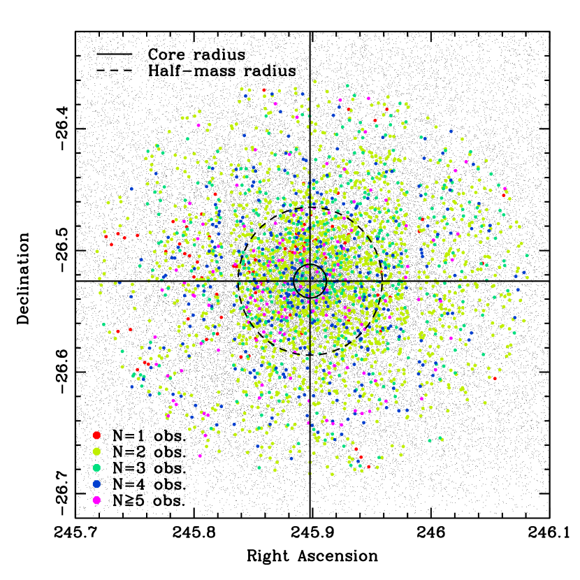
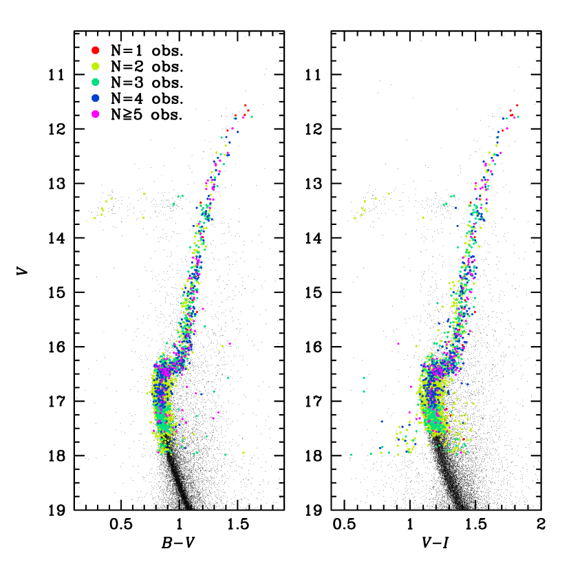
Spatial properties of our target stars are illustrated in Figure 1, where the targets are color-coded according to the number of spectra available for a given star. The cluster core radius (where the surface luminosity has decreased by a factor of two from the center) and the half-light radius are also drawn in this figure, indicating that essentially all regions of M 4 has been sampled spectroscopically. All the observed stars are inside the tidal radius of the cluster (not shown in the figures). Photometric characteristics of the stars are shown in Figure 2, here again color-coded depending on the number of observations as in Fig. 1. The two panels show the color-magnitude diagram in $V/B-V$ (left-hand panel) and $V/V-I$ (right-hand panel) before any correction for reddening. The limiting magnitude of the targets, $V~{}\lesssim$ 17.5, has been set by the requirement that a single M 4 integration had $\textrm{\mbox{SNR}}>10$ for each star in a single observation. Although Horizontal Branch stars are present in our dataset, they have been excluded from the analysis. We think that their higher temperature respect to the rest of the sample and their evolved status requires a more careful analysis that is beyond the goal of this paper.

A total of 2771 stars covering color-magnitude diagram positions from the upper red-giant branch to about one magnitude fainter than the main-sequence (MS) turnoff (TO) luminosity have been observed. The spectra span a temporal period of six years, and we refer to Sommariva et al. (2009) for a description of the observation strategy. We added 306 new spectra obtained in 2009 that targeted MS stars already observed in the previous epochs. Since these data originally were gathered to determine the M 4 velocity dispersion and to assess the binary-star fraction, nearly all stars have been observed at least twice, and three or more spectra have been obtained for nearly 40% of the sample. We summarize the observation numbers in Table 1; a total of 7250 individual spectra have been used in our study.

Sommariva et al. (2009) used the ESO GIRAFFE standard reduction pipeline (Blecha et al., 2000) to reduce the M 4 data from raw CCD exposures to final extracted, flat-fielded, wavelength-calibrated spectra. In order to maximize the information content of these spectra, we decided to revisit the reductions, paying particular attention to spectral extraction and wavelength calibration. We adapted the empirical Point Spread Function concept from photometry (Anderson & King, 2000; Anderson et al., 2006) to spectroscopy to obtain a more accurate determination of the cross-dispersion spread function of the fibres. The use of a more accurate profile results in a reduction of the noise for spectra at low SNR when using the optimal spectral extraction algorithm, as shown by Horne (1986). Wavelength calibration has been performed with an alternative technique as well. Precise RV determination from GIRAFFE data is the subject of a forthcoming paper, and it will not be discussed here.

Figure 3.— Degradation of the SNR with magnitude is shown by displaying four example spectra of stars with different magnitudes. These spectra have been chosen among the best exposed during observing runs with good atmospheric conditions and without Moon illumination.

Degradation of the SNR  with magnitude is demonstrted in Figure 3 by showing representative spectra of stars with different magnitudes. These spectra have been chosen, among target stars of similar magnitude, to be the best exposed during observing runs without Moon illumination. Other spectra at the same magnitude can have lower SNR depending on exposure times and observational conditions.

3. Overview of the Spectrum Analyses

M 4 GIRAFFE spectra have been gathered in such a way that each individual exposure has a minimum SNRgreater than 10, since this value is considered the lower limit to obtain radial velocity with a precision of a few hundreds m/s with this instrument (Sommariva et al., 2009). However, atmospheric stellar parameter and abundance derivation at stellar fluxes that are comparable to the noise level requires very careful handling of the spectra. The usual procedure is to process the observed stellar flux as much as possible in order to be comparable with the synthesis: sky contribution is subtracted, spectra are corrected by flat-fielding, normalized and finally rebinned in a linear wavelength scale. Every step in this procedure will produce an increase or an unintended correlation in the noise level of the observed spectrum. Fortunately, this problem is usually negligible when working on spectra with good SNR, but it can lead to a significant loss in precision in stellar atmospheric parameter determination when the SNR is very low This is exactly the situation we face with the majority of our observed spectra.

After many numerical experiments with our data, we adopted a new approach to handle the spectrum preparations. Specifically, after extraction and wavelength calibration of the raw spectra, we decided not to perform any subsequent data corrections. We made this choice in order to avoid introduction of any false correlations into the spectrum noise. All the steps that usually lead to sky-corrected, rest-frame, continuum-normalized stellar spectra were instead performed in the opposite direction: deliberate degradation of the “perfect” synthetic spectra to best match the real extracted spectra. Each of these steps is described in detail in the next few sections. However, application to each spectrum was done in a near-simultaneous fashion, so here we give an outline of our overall procedure, referring to the sections in which each procedure is developed.

In the following, we use the term exposure to refer to a single observation for a given star. For every exposure of the star under study, the synthesis to be compared is subject to these transformations:

• the synthesis is moved in the radial velocity space to match the measured total radial velocity shift of the exposure (i. e., star heliocentric motion plus the Earth motion);

• the level of sky flux, composed of a scattered solar (moonlight) spectrum and a gray continuum are determined (Section 4);

• the appropriate continuum slope function for the exposure is derived (Section 5):

• preliminary stellar atmospheric parameters are deduced from photometric data (Section 6):

• synthetic spectra appropriate to these parameters are computed (Section 7).

• both synthetic and solar spectra are degraded to the resolution of the instrument, determined from the Th-Ar exposures, using a Gaussian kernel;

• the synthetic spectrum, solar spectrum and gray continuum are rebinned in the wavelength scale of the exposure, keeping constant the amount of flux for unitary wavelength;

• the rebinned synthesis and sky spectra are multiplied for their continuum function, and together with the rebinned gray continuum they are linearly combined using as coefficient the corresponding flux constants, as determined in Section 4 and Section 5.

• the resulting spectrum is multiplied for the flat-field of the fiber used to gather the data to include instrumental effects, such as the characteristic efficiency curve along an order (blaze function) in echelle spectrograph.

We call the result of these operations the processed synthesis to distinguish it from the raw synthesis described in Section 7. Since every exposure differs from the others due to different observational conditions, variations in the instrument response, Moon illumination etc. this process must be performed for every exposure of a star, and any exposure can be compared only with the relative processed synthesis. As a final comment here, stars in GCs are known to be slow rotators, so the effects of possible rapid rotation are not considered in computing the the processed synthetic spectra. Nevertheless it would be very easy to incorporate this effect in the analysis, as well as determining the best fitting $v$ sin $i$ value during the $\chi^{2}$ minimization.

4. Sky flux determination

For every GIRAFFE exposure on the M 4 targets, about 5-10 fibers have been allocated to empty sky regions. Sky subtraction is usually performed by coadding the spectra from these fibers and subtracting the result from the observed spectrum of the star. There are several drawbacks when doing so:

• These spectra are intrinsically very noisy, having the sky a maximum brightness of $\simeq 17.5\,\textrm{mag}/\textrm{arcsec}^{2}$ at $30\,\mathrm{\SIUnitSymbolDegree}$ from full Moon. Even when coadded, the resulting spectrum is still very noisy, then increasing significantly the noise of the sky-subtracted spectra especially in those cases where star and sky fluxes are comparable.

• Each fiber has a different transmission efficiency. The error in its determination is propagated when the sky spectra have to be coadded, and when the coadded spectrum is subtracted from the star spectra.

• Sky spectra must be rebinned to a common wavelength scale to be coadded, then either the science spectra must be rebinned to this common scale or the coadded sky spectrum must be rebinned in the science spectra wavelength scale, in order to perform the sky subtraction correctly. The rebinning of a low SNR spectrum can introduce correlated noise and should be avoided.

• several fibers must be allocated for the sky spectra, reducing the efficiency of a multiplexing instrument such as GIRAFFE.

• even if the allocated sky fibers are scattered around the field of view, the coadded spectrum wil not be sensitive to any spatial variability of the sky and the individual spectra are too noisy and their number too low to determine it over the $\simeq 500\,\textrm{arcmin}^{2}$ covered by a MEDUSA plate.

Figure 4.— Observed spectrum of a star with $V=17.73$, obtained a few days before full Moon. The synthetic sky spectrum (red line), stellar spectrum (blue line) and a grey continuum (green line) here shown with instrumental effects already applied, are combined (magenta line) and compared to the observed stellar spectrum (black points). The upper panel shows the entire wavelength range of our spectra, while lower panel shows the Mg I b triplet region, to highlight the contribution of the sky spectrum to the observed total star+sky spectrum.

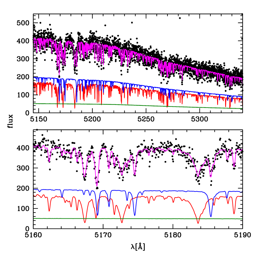
Since many of the observing runs occurred in gray/bright Moon time, the sky spectrum constitutes a significant part of the flux. An example is given in Figure 4 where the observed spectrum of a relatively faint program star ($V=17.73$) is decomposed into the stellar (blue line) and the sky (red line) contributions. The spectrum in the figure was taken on 2006 September 04, $\simeq 5$ days before full Moon and at a distance of $\simeq 40\,\textrm{deg}$. In analyzing the coadded sky spectrum we discovered that the sky light was composed of two distinct parts: one resembling the solar spectrum, due manly to the presence of the Moon, and another featureless gray one (green line).

This gray feature was first noticed in sky spectra taken during dark time, i. e.  without Moon illumination, and confirmed to be necessary when trying to fit the coadded sky spectra from Moon-illuminated nights with the solar spectrum. Intrinsic sky brightness due to zodiacal light and human light pollution (see Patat, 2008) or the presence of scattered light inside the dome are both plausible explanations. We limit ourselves to taking account of this feature, without investigating its origin.

One can see clear evidence in Figure 4 of sky contamination in the star’s low SNR spectrum, especially in the strong Mg I b lines (lower panel). We note that fortunately in our spectral range no telluric absorption lines are present, so no correction for that potential problem is needed.

The inclusion of the sky in the correct proportion with respect to the stellar flux is a fundamental part of a good synthesis match of the data. To determine the sky flux level, we proceed in the following way. The extracted and wavelength-calibrated sky spectra are corrected for fiber transmission and flat-field normalization. Then the amount of sky flux per unit wavelength is determined by integrating the sky spectra over 2 Å intervals; this value has been chosen as a good compromise between reducing the noise and preserving the main spectral features of the spectra.

In order to account for the loss of flux due to solar spectral lines, we employed the U.S. National Solar Observatory (NSO) flux atlas (Kurucz et al. 1984, Wallace et al. 2011), smoothing it to the spectral resolution of our data. This solar model is integrated in the same way as described in the preceding paragraph.

The values determined from the observed sky spectrum are fitted with a linear combination of two functions: a low-order polynomial multiplied by the values from the solar model, to take into account the Moon illumination, and a constant for the gray continuum. The resulting functions represent the continuum flux per unit wavelength as a function of the wavelength of the moon illumination and the gray continuum level, respectively. The former function is split in two parts: a constant representing the average flux of the sky, and a normalized function for the shape. We will refer to them as flux constant and continuum function respectively. Since the gray continuum is a constant, its continuum function is simply a unitary constant value (before including instrumental effects)

The coefficients of the functions as derived above represent only the first step in the sky flux derivation. During the continuum determination process, described in the next section, the flux constants are refined using the sky lines in the spectrum as a proxy, to take into account the sky variability and fiber transmission differences.

Precautions to ensure that the extra absorptions in a faint stellar spectrum are truly sky contributions and not accidental inclusion of some faint non-cluster member star in the fiber apertures have been taken. Not only must the mean sky radial velocities are consistent with a rest velocity system, but their fluxes positively must correlate with lunar phase. We have also rejected individual sky spectra that had anomalously high flux, indicative of accidental pointing at a faint star. These procedures convinced us of the real nature of the sky contaminations to our stellar spectra.

5. Continuum Normalization

Continuum rectification proved to be challenging due to the restricted total wavelength range (5140$-$5360 Å) of our spectra and to the presence of the strong Mg I b absorption lines in the first 50 Å of the spectra. The GIRAFFE HR9 setting was deliberately chosen for the original Sommariva et al. (2009) study to take advantage of the line richness in this spectral region. In addition to the Mg I b lines there are many strong Fe I lines, which makes this wavelength domain particularly attractive for radial velocity studies. But this wealth of absorption lines creates many wavelength intervals of overlapping spectral features, so defining an adequate number of points for a global continuum normalization is a very difficult task. Local normalization, usually determined by visual inspection when measuring equivalent widths, is also unsuitable for two reasons: the large number of spectra in our sample; and the subjectivity in manually selecting the continuum (which probably would have introduced a systematic bias in our lower SNR spectra). Spectral synthesis requires good normalization in the whole wavelength range of interest, and while is still feasible to manually adjust the continuum to match the synthesis when the number of stars is low, for our very large sample we had to find an alternative way.

A first estimate of the continuum stellar flux per unit wavelength is determined in a similar way as done for the sky flux. The sky and grey continuum contributions are removed from the observed spectra. Then for each star we adopt a synthetic spectrum with photometric atmosphere parameters (Section 6) and provisional metallicity $\textrm{\mbox{$[{\rm Fe}/{\rm H}]$}}=-1.15$ (Section 1) to calculate the flux constant and continuum function relative to the stellar component of the spectrum, following the same steps described in Section 4 for the sky continuum.

The synthetic stellar spectra and the solar spectra are degraded to match the spectral resolution of the instrument and together with the unitary function for the gray continuum they are rebinned into the wavelength scale of the science spectrum, keeping constant the flux per wavelength unit. All spectra are then multiplied for the corresponding continuum function and the resulting spectra are linearly combined, using the flux constants as coefficients. The instrumental effects (e. g. multiplication for flat-field) are finally applied to make the comparison with the observed spectrum possible.

The flux constants are determined by fitting the resulting model spectrum to the observed one by $\chi^{2}$ minimization (Equation 4), in the same way as we do to determine the atmosphere stellar parameters (Section 8). Small adjustments in the continuum functions also are allowed, to deal with spectral regions affected by the wings of strong spectral lines, e. g. in the proximity of the Mg I b triplet.

A binary mask is included in the $\chi^{2}$ determination to exclude points too sensitive to variations of temperature, gravity, microturbulence and metallicity. This mask is derived by taking two boundary values for each stellar parameter (i. e.  the photometric value $\pm$ its estimated error; see Section 6) and flagging those points that show a percentage variation over a fixed threshold. A detailed explanation is given in Section 8. Points that have normalized flux lower than $0.8$ in the stellar synthesis are excluded too, while the lines in the sky spectrum are retained to allow a better determination of the sky flux level.

The flux continuum functions and the flux constants are adjusted as described above for each set of stellar atmosphere parameters used during the $\chi^{2}$ determination, so that the derived values will not be influenced by the initial choice in the photometric parameters for the continuum determination. A good starting point however allows a quick recalibration of this function.

Radial velocity shifts due to the intrinsic velocity of the star and the Earth motion are applied to the stellar synthetic spectrum. No rebinning of the observed spectra is necessary, and no noise is introduced since all the operations are performed on noise-free high-resolution synthetic spectra.

6. Stellar Atmospheric Parameters from Photometry

In every minimization algorithm, a good starting point always results in a faster determination of the variable of interest. Spectral synthesis is a very lengthy process by itself, and with four parameters to be determined by $\chi^{2}$ minimization and several thousands of stars to be analyzed, this task can be excessively time-consuming. Greater speed in this process can be provided through initialization of the process with photometrically derived stellar parameters, but some precautions are necessary.

M 4 is known to have both a large mean reddening, $E(B-V)=0.34$ (Harris, 1996), and large differential reddening across its surface. We have adopded the latest determination of overall M 4 parameters derived by Hendricks et al. (2012); these are listed in Table 2.

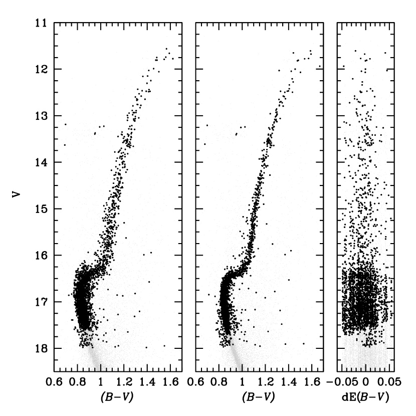
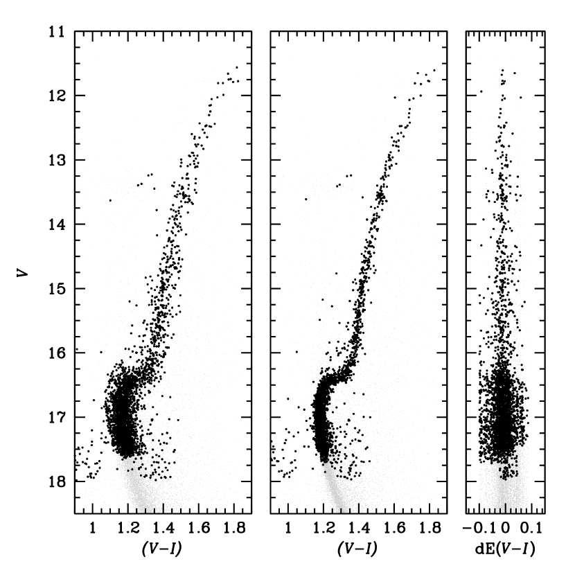
We have corrected the $B/(B-V)$ CMD for differential reddening using the technique described in Milone et al. (2012a); Here we summarize their method. The reddening direction in the CMD is defined as $\theta={\rm atan}{(A_{V}/E(B-V))}$. A subsample of the photometric catalog is identified by manually excluding those stars that lie clearly outside the cluster sequences, and including only those stars in the RGB, SGB and TO, since the angle between the reddening direction and the sequences is maximum (the reddening direction is almost parallel to the MS). A fiducial line along the RGB, SGB and TO is manually determined and then for every star in the catalog the median shift in the reddening direction with respect to the fiducial line of the 35 closest stars of the subsample is computed. This value is taken as indicative of the amount of the differential reddening, taking advantage of the fact that stars in a local spatial region (a few $\mathrm{\SIUnitSymbolArcminute}$) of M 4 all should be shifted by the same amount.

Then the $R_{V}$ value from Table 2 is used to convert dE($B-V$) to d$A_{V}$. In the same way the $V/(V-I)$ diagram has been corrected for differential reddening, to obtain a second color index whose correction is independent from the first one. Although one photometric band is in common, the two reddening corrections can still be considered independent since we are correcting an effect in color. The differential reddening-corrected CMDs in the two color combinations for our target stars are shown in Figure 5 and Figure 6, along with the amount of correction as a function of magnitude. The overall cluster reddening correction (Table 2) has not been applied here yet.

Figure 5.— The $V/(B-V)$ diagram before (first panel) and after (second panel) the differential reddening correction, with the cluster stars in gray and target stars highlighted in black. The third panel shows the amount of the correction. The overall mean reddening correction has not been applied yet.

Figure 6.— As in Figure 5, for the $V/(V-I)$ plane.

The two color indices have been used to obtain two estimates of the (photometric) stellar atmosphere parameters, using the calibrations described in the next subsections. Although very precise, we must keep in mind that these value will be used only as input values for our spectroscopic determination.

6.1. Effective Temperatures

For every star two independent values for effective temperatures are obtained from $(B-V)$ and $(V-I)$ colors using the relations from Ramírez & Meléndez (2005) for giant stars and Casagrande et al. (2010) for subgiants and dwarfs stars. The switch between the two relations has been set at $V^{switch}=16.1$, as described below.

Figure 7.— Differences in derived effective temperature using the colors $(B-V)_{0}$ and $(V-I)_{0}$. The upper panels show the temperature differences when using the calibration for giant (left-hand panel) and dwarf (right-hand panel) stars. Equality of temperatures is represented by the green lines. Switching the calibration at $V=16.1$ provides the lower scatter in the difference when considering giant (red points) and dwarf (blue points) stars together (lower panel).

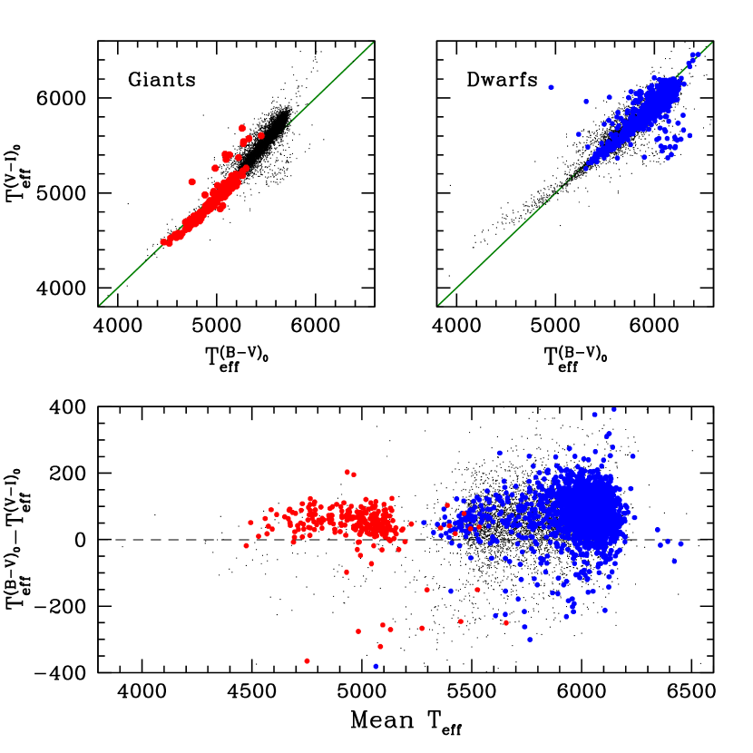
The differences in derived effective temperature using the two colors are shown in Figure 7. The two upper panels show direct comparisons between the derived temperatures using the two colors, for giants stars in the left-hand panel and dwarfs/subgiants in the right-hand one. The threshold of the switch has been chosen by looking where the two temperatures begin to differs systematically, i. e.  the points start to deviate from the green lines. The lower panel shows the difference of the color-derived temperatures with respect to their mean, which is the value that will be used to derive the other stellar parameters. A gap around $\textrm{$T_{{\rm eff}}$}\simeq 5200\,\mathrm{K}$ is clearly visible: Casagrande et al. (2010) report a systematic difference of $\simeq+100\,\mathrm{K}$ with the calibration of Ramírez & Meléndez (2005) for dwarf stars, and probably such difference is affecting also the calibrations for giant stars. We did not attempt to correct this difference, letting the parameter determination algorithm solve it.

Figure 8.— The variations in temperature as a function of dE($B-V$) and dE($V-I$) can be used as the corrections in temperature due to the differential reddening correction, or as the error in temperature for a given error in color. Values have been determined using a metallicity of $\textrm{\mbox{$[{\rm Fe}/{\rm H}]$}}=-1.15$.

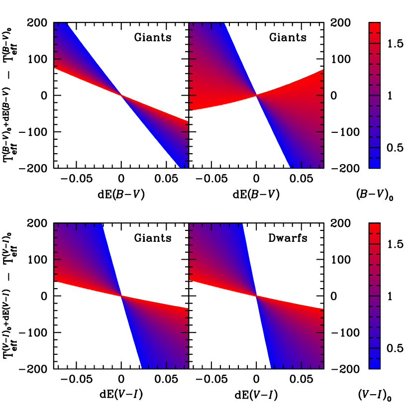
It is interesting to see the dependence of temperature on small variations of colors, as given by the calibration. Figure 8 shows the difference between the temperature derived from the cited calibrations when using a given input color (color-coded according to the bar on the right) and the temperature obtained after including some color excess (horizontal axis of the plots) to the considered color. Calculations have been performed for both giant and dwarf stars, using respectively Ramírez & Meléndez (2005) and Casagrande et al. (2010) calibrations, for the two colors at our disposal and a metallicity of $\textrm{\mbox{$[{\rm Fe}/{\rm H}]$}}=-1.15$. The variations in temperature as a function of dE($B-V$) and dE($V-I$) can be used as the correction in temperature due to the differential reddening correction, or as the error associated to temperature for a given error in color. Note that for a given star the temperature derived using the $(V-I)$ color is in general more sensitive to small variations than using $(B-V)$, but usually the reddening correction is more reliable when using passbands close to the infrared. These two effects counterbalance to give similar errors in the temperatures derived from the two colors. From the scatter in the difference between the temperatures derived using the two colors , we estimate an average error of $\textrm{$T_{{\rm eff}}$}=150\,\mathrm{K}$ for photometric derived temperatures.

6.2. Surface Gravities

Photometric gravities are calculated from the classical relation:

$$\begin{split}\textrm{\mbox{log~{}{\it g}}}^{\star}&=\textrm{\mbox{log~{}{\it g}}}^{\odot}+4\log\frac{\textrm{$T_{{\rm eff}}$}^{\star}}{\textrm{$T_{{\rm eff}}$}^{\odot}}\\ &+0.4(M_{V,*}+\textrm{BC}-M_{\rm bol,\odot})+\log\frac{M_{*}}{M_{\odot}}\end{split}$$ (1)

where we have adopted a distance of $1.8\,\mathrm{k}pc$ (Table 2) to relate the reddening-corrected relative magnitudes to absolute $V$ magnitudes $M_{V,*}$. A mean mass of $M_{\star}=0.85M_{\odot}$ has been assumed. For every star the bolometric correction is obtained interpolating the table from Houdashelt et al. (2000) for the values of temperature and gravity of the star and iterating over $\textrm{\mbox{log~{}{\it g}}}_{*}$ until convergence is reached. Canonical solar values $\textrm{$T_{{\rm eff}}$}^{\odot}=5770K$, $\textrm{\mbox{log~{}{\it g}}}^{\odot}=4.44$, $M_{\rm bol,\odot}=4.75$ (see for example Cox & Pilachowski 2000) have been adopted.

6.3. Microturbulent Velocities

Initial values of microturbulent velocities for stars cooler than $5000\,\mathrm{K}$ are derived using the relation from Marino et al. (2008):

$$\textrm{\mbox{$\xi_{\rm t}$}}=-0.254*\textrm{\mbox{log~{}{\it g}}}+1.930$$ (2)

This relationship has been derived from giants stars in M 4, but it might not be suitable for dwarf stars. For dwarf stars we initially used the relation from Gratton et al. (1996):

$$\textrm{\mbox{$\xi_{\rm t}$}}=1.190*10^{-3}*\textrm{$T_{{\rm eff}}$}-0.900*\textrm{\mbox{log~{}{\it g}}}-2.00$$ (3)

The two calibrations have similar values at $\simeq 5100K$, or $\textrm{\mbox{log~{}{\it g}}}=3.1~{}\textrm{dex}$

Figure 9.— Calibration of microturbulence as a function of gravity from Gratton et al. (1996) (black points) and Marino et al. (2008) (red points) for our target stars. The first calibration is also dependent on temperature, hence the spread in the plot.

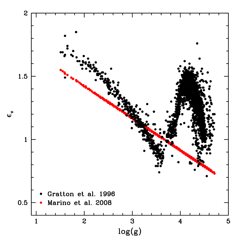
As discussed later, several problems have been encountered while determining the microturbulent velocities of dwarf stars. We finally decided to use the velocities computed by Equation 2, given the fact that these values are used only for the first iteration of stellar atmosphere parameters determination.

7. Spectral synthesis

The first ingredient for a good spectral synthesis is a list of spectral lines as accurate and complete as possible. All the atomic lines in the spectral range 5140$-$5360 Å have been collected from several sources in literature, see Kurucz (1995), Sobeck et al. (2007), Lawler et al. (2007), Lawler et al. (2009), Biémont et al. (2011), Roederer & Sneden (2011) and references therein. The listed values for the oscillator strength log gf of each line are usually the results of laboratory experiments or semi-empirical estimates. Calculated log gf’s from theory may be subject to large uncertainties, which fortunately can be corrected in numeric experiments with astrophysical spectra.

We have used the NSO Solar Atlas (Kurucz et al. 1984, Wallace et al. 2011) and the Atlas of Arcturus Spectrum (Hinkle et al. 2000) to improve the transition probabilities in our line list. For the Sun we have assumed the standard atmospheric parameters $\textrm{$T_{{\rm eff}}$}=5777\,\mathrm{K}$ , $\textrm{\mbox{log~{}{\it g}}}=4.44$, $\textrm{\mbox{$\xi_{\rm t}$}}=1.5\,\mathrm{k}\mathrm{m}/\mathrm{s}$ , $\textrm{\mbox{$[{\rm Fe}/{\rm H}]$}}=0.00$. For Arcturus there is no general consensus on the atmospheric parameters. We have decided to use the values listed by Massarotti et al. (2008) which are $\textrm{$T_{{\rm eff}}$}=4325\,\mathrm{K}$, $\textrm{\mbox{log~{}{\it g}}}=2.1$, $\textrm{\mbox{$\xi_{\rm t}$}}=2.0\,\mathrm{k}\mathrm{m}/\mathrm{s}$ , $\textrm{\mbox{$[{\rm Fe}/{\rm H}]$}}=-0.60$. The model atmospheres are generated by interpolation in the Kurucz (1992) model atmosphere grid calculated with the “New Opacity Distribution Function” (ODFNEW, Castelli & Kurucz 2004). The syntheses are generated using the current version of the Local Thermodynamic Equilibrium (LTE) code MOOG (Sneden, 1973). Oscillator strength values have been modified iteratively until synthetic spectra produced satisfactory matches with the observed solar and Arcturus spectra. When it was not possible to find a value to match both spectra satisfactorily, priority has been given to the Solar one, given the uncertainty in the stellar parameters and chemical composition of Arcturus. In some cases it has been necessary to add some atomic lines with arbitrary parameters in order to reproduce the solar spectra in places where there is no known atomic or molecular identification. These fake lines have been chosen to be Fe I transitions with excitation energies of 3.5 eV and gf-values adjusted to match the observed spectral features. While these lines have been excluded in the atmospheric parameter determination, their inclusion in the synthesis ensure a more reliable determination of the continuum.

Figure 10.— The improvement on spectral synthesis from before (red line) and after (blu line) the refinement of the log gf values in the input line list, compared with high SNR spectrum of the Sun (upper panel) and Arcturus (lower panel).

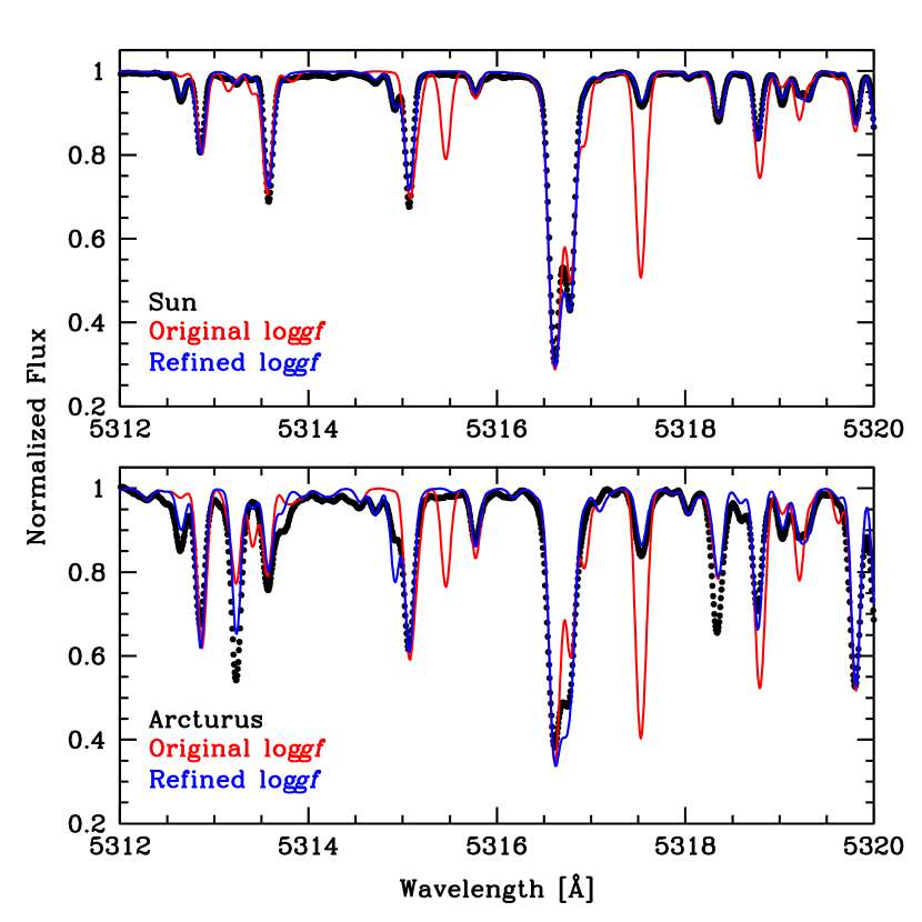
Figure 10 shows the improvement in the synthesis from before (red line) and after (blue lines) the refinement of log gf values. For the Sun the improved line list causes a reduction of the dispersion of the synthesis respect to observed points from $\sigma=0.0507$ to $\sigma=0.0147$, while for Arcturus we have a reduction from $\sigma=0.0688$ to $\sigma=0.0336$. Further improvement in the dispersion can be achieved by noting that Arcturus has a non-solar abundance distribution (e. g., Peterson et al. 1993, Ramírez & Allende Prieto 2011). In Figure 10 it is clear that the observed spectrum depths exceed the computed ones for transitions near 5313.2 Å and 5318.3 Å. The species responsible for these absorption features are Ti I at 5313.24 Å and Sc II at 5318.36 Å. Both Ti and Sc are overabundant by 0.2$-$0.3 dex with respect to Fe in Arcturus (Ramírez & Allende Prieto 2011), while the synthesis have been generated using solar-scaled abundances. Accounting for those overabundances would essentially erase the observed/synthesized mismatches at these wavelengths.

The syntheses for M 4 stars have been generated again using the Castelli-Kurucz (Kurucz, 1992) model atmospheres based on opacity distribution functions, this time with $\alpha$-element abundance enhancements (AODFNEW, Castelli & Kurucz 2004). The interpolator code was kindly provided to us by Andy McWilliam and Inese Ivans. We modified this code so that the synthesis program automatically set the abundance of the $\alpha$ elements to the ones measured by Ivans et al. (1999), namely $\log\epsilon(\mathrm{O})=7.68$, $\log\epsilon(\mathrm{Mg})=6.52$, $\log\epsilon(\mathrm{Si})=6.60$, $\log\epsilon(\mathrm{Ca})=5.12$, $\log\epsilon(\mathrm{Ti})=3.79$ for $\textrm{\mbox{$[{\rm Fe}/{\rm H}]$}}=-1.15$, with those values scaled accordingly with $[{\rm Fe}/{\rm H}]$.

Since many stars in our sample share similar temperatures, gravities and microturbulent velocities, to speed up the determination of the atmosphere parameters we have created a grid of synthetic spectra with a spacing of $100\,\mathrm{K}$ in temperature, $0.1$ in gravity, $0.1\,\mathrm{k}\mathrm{m}/\mathrm{s}$ in microturbulent velocity and $0.05$ in metallicity. The grid is built on the photometric atmospheric parameters derived for all the stars in the sample. For a specific set of parameters, the synthesis is computed by linear interpolation of the syntheses with the closest parameters within the spacings of the grid.

8. Stellar parameters and abundance analysis

In this section we discuss the algorithms used to iteratively determine $T_{{\rm eff}}$, log g, $\xi_{\rm t}$, and $[{\rm Fe}/{\rm H}]$ for each M 4 target star.

Suppose that we have a star with $n_{obs}$ exposures, each one with $n_{pixel}$ flux points $F(n,i)$ for the exposure $n$ at the pixel $i$ and its associated wavelength value. For each set of atmosphere parameters we can calculate the $\chi^{2}$ as given in Equation 4:

$$\chi^{2}=\frac{\sum_{n=1}^{n_{obs}}\sum_{i=1}^{n_{pixels}}\frac{(F(n,i)-S_{o}(n,i))^{2}}{S_{o}(n,i)}p(n,i)w(n,i)}{\sum_{n=1}^{n_{obs}}\sum_{i=1}^{n_{pixels}}p(n,i)w(n,i)}$$ (4)

where $p(n,i)$ is a binary mask to include only points sensitive to the atmospheric parameter of interest, $w(n,i)$ is a weight function and $S_{o}(n,i)$ is the value of the processed synthesis, each of them relative to exposure $n$ at the pixel $i$. $S_{o}$ is a function not only of the stellar parameters, but also of the polynomial coefficients for the flux continuum, which are determined uniquely for each set of stellar parameters. The final set of atmosphere parameters will be the one that minimizes the $\chi^{2}$. The masks and weights need to be discussed now in more detail.

Atmosphere parameter masks

Although there are no lines affected only by a single parameter, every line reacts differently to a change of one of them. To determine which pixels are more sensitive to a specific parameter compared to the others, we created several masks, applying sequentially the following scheme for each stellar parameter:

• two extreme values based roughly on the expected photometric errors are chosen for the atmospheric parameter under analysis;

• two syntheses with the extreme values of this parameter are calculated, with the other parameters kept fixed to the photometric values;

• when the difference between the two synthesis is more than 5% (10% for metallicity), the binary mask is assigned a positive value, otherwise it is declared to be null.

The ranges used for masks creation are $\Delta\textrm{$T_{{\rm eff}}$}=\pm 150\,\mathrm{K}$, $\Delta\textrm{\mbox{log~{}{\it g}}}=\pm 0.5$, $\textrm{\mbox{$\xi_{\rm t}$}}=\pm 0.5\,\mbox{km s${}^{-1}$}$, and $\textrm{\mbox{$[{\rm Fe}/{\rm H}]$}}=\pm 0.5$.

The metallicity mask is actually used only to exclude from the continumm the points that are affected by a change in the overall metallicity (i. e. spectral lines). Although the continuum is being determined as a part of every synthesis/observation comparison, we want to minimize as much as possible the influence of spectral features. The continuum mask has positive value only when all the other masks have corresponding null values.

An additional mask is created using the Fe I lines from the line-list provided by Ivans et al. (2006) and Sousa et al. (2011). These lines have been selected for Equivalent Width measurements in high resolution spectra (respectively HIRES and HARPS), and their astronomical log gf values have been carefully determined. This mask is the one used in the determination of the $[{\rm Fe}/{\rm H}]$ value.

Since the phometric values of the atmospheric parameters are reasonably close to the ones finally derived in our analyses, we do not expect any significant change between the mask obtained with the photometric value and the one that we would obtain if the real atmosphere parameters were already known.

Weight function

The weight function $w(n,i)$ is basically a correction factor to give more importance to the stellar lines with respect to the sky ones in the $\chi^{2}$ determination. For every atmospheric parameter two extreme values are selected around the photometric value (namely, $\Delta\textrm{$T_{{\rm eff}}$}=\pm 200\,\mathrm{K}$, $\Delta\textrm{\mbox{log~{}{\it g}}}=\pm 0.5$, $\Delta\textrm{\mbox{$\xi_{\rm t}$}}=\pm 0.5km/s$), a synthesis is generated for every combination of the parameters, and for every wavelength point in the synthesis the lowest and highest values from all the syntheses are saved. Hereafter we refer to these two spectra simply as minimum and maximum spectra.

The two spectra are translated to the observational space as explained earlier, including the addition of the sky background. We define a selection strip by adding the expected Poissonian noise multiplied by two to the processed maximum spectrum, and subtracting the Poissonian noise multiplied by three to the processed minimum one. We use a lower factor for the upper limit because the range of variation of a spectrum is set by its continuum, so outliers are easier to identify and a tighter constraint can be used. The Poissonian noise is computed using the overall (sky and star) continuum level.

All the points outside the strip are excluded from the $\chi^{2}$ computation, as well as data points flagged as unusable during spectral extraction, by giving them null weight.

With this procedure, we are able to safely exclude undetected lines, anomalous pixel values (e. g. due to anomalous measurement of flux or inaccurate flat-field correction) and cosmic rays that survived to the optimal extraction or have not been flagged properly.

The weight is determined using Equation 5:

$$w(i,n)=\sqrt{2-(S_{syn}^{max}(i,n)-S_{syn}^{min}(i,n))/2}$$ (5)

where $S_{syn}^{max}$ and $S_{syn}^{min}$ are respectively the maximum and the minimum spectra before being processed. With the weight defined in this way, more importance is given to the line belonging only to the stellar spectrum while the global fit is preserved, resulting in an improved atmosphere parameter determination.

Figure 11.— The same spectrum in Figure 4 is shown (black points for the observed spectrum and magenta for the synthesis), with the upper boundary (blue line) and the lower one (red) highlighted. Points that have been excluded from the $\chi^{2}$ determination are flagged in orange. The green line represents the weight function $w(i,n)$, multiplied by a factor of 50.

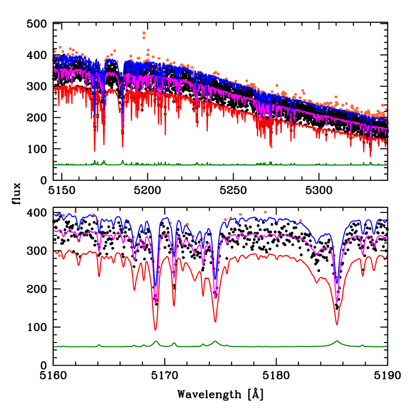
In Figure 11 the selection strip is shown. Points excluded from the $\chi^{2}$ determination have been flagged in orange. A green line shows the weight function resulting from Equation 5, multiplied of a factor of 50.

We decided to perform this selection before the $\chi^{2}$ determination and not during the synthesis-observation comparison, i. e. using the photometric values as reference instead of the actual synthesis as a proxy, since the inclusion or exclusion of different points or a change of the value of the weights during the $\chi^{2}$ determination can affect the final results.

$\chi^{2}$ minimization and atmosphere parameters determination

Due to the complex interdependence of the atmosphere parameters, we have opted for a simple but robust method for the $\chi^{2}$. Each iteration is characterized by a set of input values of $T_{{\rm eff}}$, log g, $\xi_{\rm t}$  and $[{\rm Fe}/{\rm H}]$; in the first iteration the inputs are the photometric values. Each parameter is varied individually while the other are kept fixed at their input values, and the value that minimize the $\chi^{2}$ of the variable parameter is saved in the output set. A new set is generated by adding to each of the parameters of the input set half of the difference between output and input set parameters, and the resulting values are taken as the new input value for the next iteration. The cycle is broken when the difference input and output set parameters are $<15\,\mathrm{K}$ for temperature, $<0.05\,\mathrm{k}\mathrm{m}/\mathrm{s}$ for microturbulent velocity and $<0.05~{}\textrm{dex}$ for the other parameters, with all these conditions to be satisfied simultaneously. If convergence is not reached, determination is considered unsuccessful and the star is dropped.

At every iteration of the algorithm a new set of atmosphere parameters is generated, and a synthesis with these parameters must be obtained to proceed with the $\chi^{2}$ minimization. The synthesis is calculated by linear interpolation of the pre-existing grid of spectra introduced in Section 7. If the required syntheses are not included in the grid, they are generated at run-time and included in the grid. With this expedient only the synthesis needed by the program are created, optimizing the coverage of the parameters space against the time spent to create such grid.

9. Results

9.1. Stellar atmosphere parameters and average metallicity

The techniques described above are applied to determine the stellar atmosphere parameters $T_{{\rm eff}}$, log g, $\xi_{\rm t}$ and $[{\rm Fe}/{\rm H}]$ of our initial set of 2771 program stars. Of these stars, 2570 have reliable radial velocities, and 1910 have spectra of sufficient quality to determine the atmosphere parameters without any arbitrary constraints.

Figure 12.— Metallicity as a function of $V_{0}$ magnitude is shown here. The average derived metallicity for RGB stars, i. e. stars with magnitude $V_{0}<14.7$ and color $(B-V)_{0}>0.70$, is nearly constant. However, fainter/bluer SGB and MS/TO stars have significantly lower metallicities with higher star-to-star metallicity dispersion. See text for discussion.

Figure 13.— The trend of effective temperature (upper plot), gravity (middle plot) and microturbulent velocity (lower plot) as a function of color $(B-V)_{0}$. The jump at $(B-V)_{0}\simeq 0.70$ is probably due to the unreliable determination of $\xi_{\rm t}$, which in turn is affecting the other parameters during the $\chi^{2}$ minimization

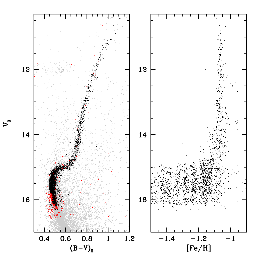
The color-magnitude of the stars with successful determinations is shown in Figure 12 (left-hand panel). Stars for which the algorithm failed in finding the atmosphere parameters are marked as red. The trend of derived metallicity is shown in the right-hand panel. For stars with $V_{0}<14.7$ we have an average value for metallicity of $\textrm{\mbox{$[{\rm Fe}/{\rm H}]$}}=-1.068\pm 0.001~{}\textrm{dex}$ and a dispersion around the mean of $\sigma=0.025~{}\textrm{dex}$, with the quoted values referring to internal random errors only (systematics can be as high as $0.1~{}\textrm{dex}$). This value, derived using 322 stars along the RGB, is in good agreement with $\textrm{\mbox{$[{\rm Fe}/{\rm H}]$}}=-1.07\pm 0.01~{}\textrm{dex}$ determined by Marino et al. (2008) (M08). That study derived metallicities of 105 M 4 RGB stars ($V_{0}\geq 12.6$) from high-resolution UVES spectra, using EW-based abundance analyses. A more detailed comparison of the atmospheric parameters for the 100 stars in common with M08 is shown in Fig. 14. The main difference (in the sense M08 minus this study) and the relative dispersion for each atmospheric parameter are $\Delta\textrm{$T_{{\rm eff}}$}=-54\ \mathrm{K}$, $\sigma_{\Delta\textrm{$T_{{\rm eff}}$}}=62\ \mathrm{K}$; $\Delta\textrm{\mbox{log~{}{\it g}}}=0.45$, $\sigma_{\Delta\textrm{\mbox{log~{}{\it g}}}}=0.16$; $\Delta\textrm{\mbox{$\xi_{\rm t}$}}=-0.003\mathrm{k}\mathrm{m}/\mathrm{s}$, $\sigma_{\Delta\textrm{\mbox{$\xi_{\rm t}$}}}=0.088\mathrm{k}\mathrm{m}/\mathrm{s}$; $\Delta\textrm{\mbox{$[{\rm Fe}/{\rm H}]$}}=-0.025$, $\sigma_{\Delta\textrm{\mbox{$[{\rm Fe}/{\rm H}]$}}}=0.090$.

Figure 14.— Comparison between the atmospheric parameters and metallicities obtained in (Marino et al., 2008) with the one obtained in this work, for the 100 stars in common between the two samples.

Gravity is the only parameter that differs significantly from M08; this could be explained by the lack of Fe II lines in our wavelength range. The main driver for the gravity determination in our technique are the wings of the Mg I b triplet, which could be affected by an incorrect value assumed for the Mg abundance. Gravity however seems to have a little influence on the determination of the other parameters; in fact assuming for gravity a value derived with different assumed stellar masses or distances in Equation 1 does not produce different results for the other parameters. This is likely due to the high number of spectral lines belonging to neutral elements (mostly Fe I and Ti I) which are insensitive to gravity in our temperature range.

This overall concordance suggests that our approach to continuum determination and parameter estimation is reliable.

For 1588 stars fainter than $V_{0}=14.7$ (bluer than $(B-V)_{0}\simeq 0.70$) the derived mean metallicity decreases fairly abruptly to $\textrm{\mbox{$[{\rm Fe}/{\rm H}]$}}=-1.162\pm 0.002~{}\textrm{dex}$, and the dispersion in metallicity increases just as quickly to $\sigma=0.18~{}\textrm{dex}$. This behavior can be better understood by analyzing the trend of the other stellar parameters with color.

In Figure 13 we have plotted derived values of $T_{{\rm eff}}$, log g, and $\xi_{\rm t}$ as functions of $(B-V)_{0}$. It can be seen that at bluer colors (higher $T_{{\rm eff}}$ values, larger magnitudes), i. e. at lower SNR, the derivation of microturbulent velocity becomes unreliable, with a huge dispersion that is not easily explainable from a physical point of view. It is intrinsically difficult to derive $\xi_{\rm t}$ in M 4 MS/TO and SGB stars because (a) the weak lines that were on the linear part of the curve-of-growth in RGB stars now disappear into the higher spectroscopic noise (Fig. 3), and (b) the lines that were strong in RGB stars now often weaken toward the linear power curve-of-growth, losing their sensitivity to $\xi_{\rm t}$. The combination of these two effects causes a reduction of independent data points, i. e., points that are more sensitive to one stellar atmospheric parameter than the others. The fitting procedure is not able to break the degeneracy between $\xi_{\rm t}$ velocity and the other parameters, settling down to a set of values dependent on their initial values and the path followed by the $\chi^{2}$ minimization algorithm. This effect can be seen also in the jump in $T_{{\rm eff}}$ in conjunction with the point where $\xi_{\rm t}$ stops following a defined trend at $(B-V)_{0}\simeq 0.70$. Indeed that point corresponds to the points where the SGB joins the RGB.

Figure 15.— Correlations of $[{\rm Fe}/{\rm H}]$ as function of $\xi_{\rm t}$ for stars with $(B-V)_{0}<0.7$ and $V_{<}14.7$. A strong trend of metallicity with microturbulent velocity is present for these MS/TO and SGB stars.

Incorrect derivations of stellar parameters of course affects the determination of metallicity, and Figure 15 shows the clear correlation of $[{\rm Fe}/{\rm H}]$ with the microturbulence velocity for MS/TO and SGB stars. Unfortunately there appears to be no reliable calibration in the literature of $\xi_{\rm t}$ as a function of colors and magnitude for these kinds of stars.

Figure 16.— Atmospheric parameters after combining giants with $\xi_{\rm t}$ as a free parameter and dwarfs with fixed $\xi_{\rm t}$. The transition between the two groups in temperature and gravity is now smoother.

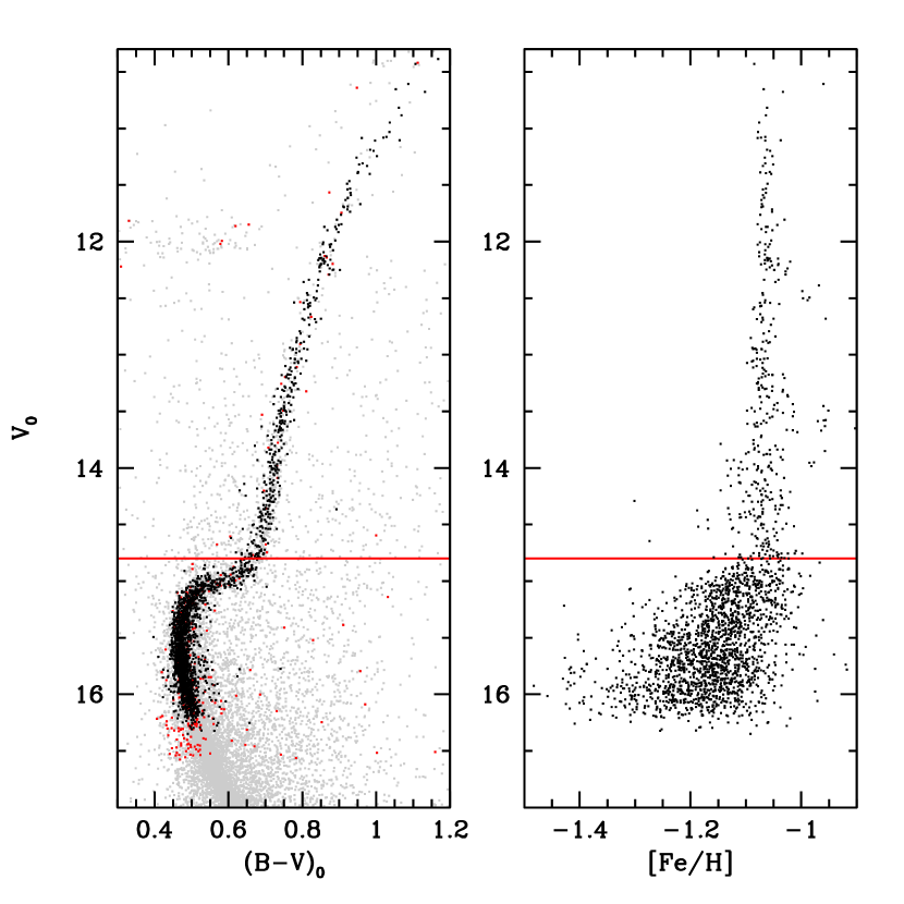
We decided to fix at $\textrm{\mbox{$\xi_{\rm t}$}}=0.7\,\mathrm{k}\mathrm{m}/\mathrm{s}$ the microturbulence for stars with $V_{0}>14.7$. This value has been derived according to the trend of $\xi_{\rm t}$ defined by the RGB stars, extrapolated to the SGB and MS/TO regime. With this constraint, the number of stars successfully analyzed grows from 1910 stars to 2191, of which there are 322 RGB and 1869 SGB and MS/TO stars. The resulting atmosphere parameters are shown in Figure 16. The transition between the two groups is now smooth.

Figure 17.— Metallicity as a function of $V_{0}$ magnitude is shown here. For MS/TO and SGB stars a microturbulent velocity of $\textrm{\mbox{$\xi_{\rm t}$}}=0.7\,\mathrm{k}\mathrm{m}/\mathrm{s}$ has been assumed (stars under the red line). The average metallicity for MS and SGB stars, $\textrm{\mbox{$[{\rm Fe}/{\rm H}]$}}=-1.16~{}\textrm{dex}$, is significantly lower than RGB stars. Assuming different values for $\xi_{\rm t}$ does not reduce significantly this difference.

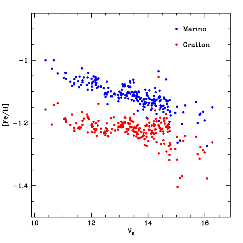
Before opting to use a fixed value for microturbulent velocity, we have checked if Equations  2 or  3 could be used to fix this parameter for all the stars in the sample. Figure18 shows that when using Equation 2 (blue points) the derived metallicities have a marked trend with magnitude already at the level of RGB stars, while the metallicities derived by using Equation 3 (red points) are systematically lower than the ones obtained either from equivalent width analysis or when leaving the microturbulent velocity as a free parameter for giant stars.

Figure 18.— Resulting metallicities when using Equations  2 (blue points) and  3 (red points). The presence of trends and systematics offsets with literature values convinced us to leave the microturbulent velocity as a free parameter for giant stars

Finally the trend of metallicity with magnitude is shown in Figure 17. The mean metallicity measured from MS and SGB stars is significantly lower than the one measured from RGB stars. From 1869 stars with $V_{0}>14.7$, we have an average metallicity of $\textrm{\mbox{$[{\rm Fe}/{\rm H}]$}}=-1.162\pm 0.002~{}\textrm{dex}$, with a dispersion of $\sigma=0.09~{}\textrm{dex}$. We have tested several values for the microturbulence velocity and we find that a positive variation of $0.1$ dex in $\xi_{\rm t}$ causes a net change of $\simeq-0.01$ dex in the derived metallicity. Thus it cannot explain the $0.10$ difference between the S/SGB and the RGB samples.

Whether this metallicity trend is a consequence of the difficulties we have in extracting abundances at these very low SNR levels, or a real result (as suggested for other clusters, see, e.g., Lind et al. 2008) shall be further investigated.

Our overall metallcity scale for M4 is dependent on a large number of choices that we have made in reduction of observed spectra, generation of synthetic spectra, and the matching of them. In earlier sections of this paper we have discussed our analytical decisions in detail. However, as emphasized in, e. g., Kraft & Ivans (2003), all abundance analyses are tied to their adopted methodologies. In Table 3 we gather many of the M 4 metallicity estimates from the literature. This list is probably not complete, and concentrates on more recent $[{\rm Fe}/{\rm H}]$ values. Neglecting the early small-sample study of Geisler (1984), the mean of the remaining 18 literature values is $<$$[{\rm Fe}/{\rm H}]$$>=-1.18$, with $\sigma=0.08$; the extreme values range from $-1.05$ to $-1.32$. Our derived values of $-$1.07 (SGB/RGB stars) and $-1.16$ (MS/SGB stars) are consistent with the literature. Note that Monaco et al. (2012) derive metallicities for their M4 MS stars that are 0.14 dex smaller than those of their SGB/RGB sample. This is in the same sense and about the same magnitude as we find between our MS/SGB and SGB/RGB stars.

Although we still suspect that analytical difficulties attend the derivation of reliable metallicites for our low SNR spectra of the MS/SGB group, it is possible that other factors may be contributing to the small mean $[{\rm Fe}/{\rm H}]$ shift seen here. More investigations on this point are required.

9.2. $\alpha$-elements and metallicity

To test the influence of $\alpha$-elements on the determination of metallicity, we have varied all the abundances listed in section 7 by $\pm 0.1~{}\textrm{dex}$ and performed again our analysis on a subset of stars randomly selected along the sequences in the CMD.

Figure 19.— The influence of the assumed abundances for $\alpha$-elements (section 7) on the determination of metallicity is tested by varying the quoted values of $\pm 0.1~{}\textrm{dex}$ and determining again the atmospheric parameters and metallicity.

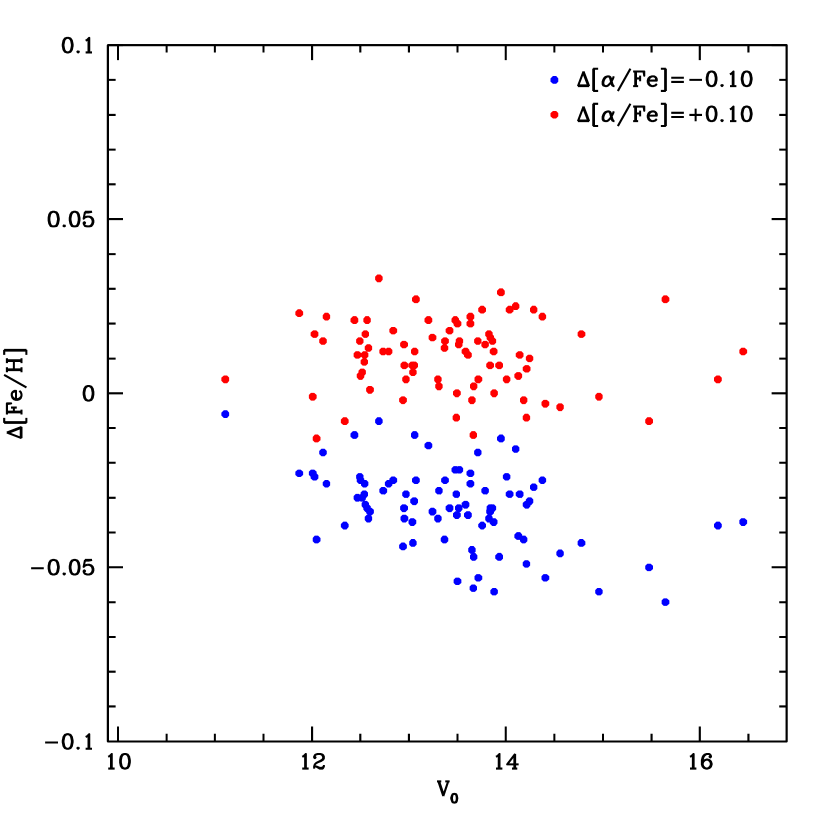
Figure 19 shows that a $+0.1\textrm{dex}$ variation in alpha elements corresponds to an average increase in $[{\rm Fe}/{\rm H}]$of $0.01~{}\textrm{dex}$, while the same variation of $\alpha$-elements in the opposite direction is causing a decrease in metallicity of $\pm 0.03~{}\textrm{dex}$. Since the difference between the true abundances of $\alpha$-elements and the ones derived by Ivans et al. (1999) is likely smaller than the variation we have used to test their influence on metallicity, and being this difference one order of magnitude smaller than other systematics effects, we can safely state that our results are independent of the exact choice of $\alpha$-elements abundances.

9.3. Metallicity of the multiple sequences

The existence of two sequences in the RGB of M 4 has been demonstrated spectroscopically by M08 and subsequently observed photometrically by Monelli et al. (2013) (MO13) on a larger sample of stars by using an appropriate combination of photometric filters. To determine if there is any difference in metallicity between the two sequences, we have cross-matched their selection (upper panels of Figure 4 in MO13) with our catalogue. Here we are retaining the same color code and naming convention used in MO13 to distinguish the two sequences, i. e.green for RGBa and magenta for RGBb. The cross-match results in 99 stars for RGBa and 207 stars for RGBb.

Before determining the mean metallicity of each sequences, we have decide to empirically correct for linear trends of $[{\rm Fe}/{\rm H}]$ with magnitude to better highlights systematic differences between the two sequences. By fitting all the stars in the RGB (blue line in the left panel of Figure 20) we have found a linear trend of $-0.0044~{}\textrm{dex}/\textrm{mag}$ with the zero point at $V_{0}=13.0,~{}\textrm{\mbox{$[{\rm Fe}/{\rm H}]$}}=-1.0677$. Both RGBa and RGBb stars have been corrected for the same trend before the determination of the mean metallicity. From our data it is not possible to determine if this trend is caused by a systematic effect of model atmosphere with temperature or by our analysis technique, e. g.a non-perfect continuum normalization. This trend however is so tiny that it does not influence our previous discussion.

Figure 20.— Left Color-magnitude diagram resulting from the cross-match of our sample with Monelli et al. (2013) database for the two RGB sequences. We used the same color code and naming convention (green for RGBa and magenta for RGBb) as in Monelli et al. (2013). The blu line represents the slope use to empirically remove the trend of metallicity with magnitude. Right. Normalized distribution in $[{\rm Fe}/{\rm H}]$for the two stellar populations. The gray lines represent the median of each distribution.

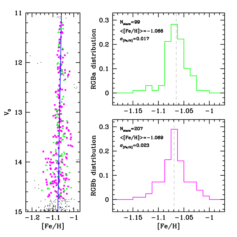
The histograms of the two normalized distributions are shown in the left panels of Figure 20. We find a median metallicity of $\textrm{\mbox{$[{\rm Fe}/{\rm H}]$}}^{RGBa}=-1.066$ with a dispersion (determined as the 68^st of the residuals from the median) of $\sigma^{RGBa}_{\textrm{\mbox{$[{\rm Fe}/{\rm H}]$}}}=0.017$ for the sequence RGBa, and $\textrm{\mbox{$[{\rm Fe}/{\rm H}]$}}^{RGBb}=-1.069$ with $\sigma^{RGBb}_{\textrm{\mbox{$[{\rm Fe}/{\rm H}]$}}}=0.023$ for the second sequence. With a Spearman’s rank correlation coefficient of $-0.19$ and an error on the mean metallicity of each sequence lower than $0.002~{}\textrm{dex}$, we conclude that no difference in metallicity between the two sequences is visibile at a level of $0.01~{}\textrm{dex}$.

10. Conclusions

We have presented here a new algorithm to automatically determine the continuum normalization level for spectra characterized by a very short and almost continuum-less wavelength range, very low SNR and strong contamination from sky background. We have coupled this algorithm with a modified $\chi^{2}$ minimization algorithm for the derivation of stellar parameters by comparison with spectral syntheses. Data points have been weighted according to the sensitivity of spectral features with respect to variations in the atmosphere parameters.

The robustness of our algorithm has been tested over 322 RGB stars down to $V\simeq 16$ resulting in an almost constant metallicity along the entire RGB and an average value of $\textrm{\mbox{$[{\rm Fe}/{\rm H}]$}}=-1.068\pm 0.001~{}\textrm{dex}$, consistent with the one derived in Marino et al. (2008) from 105 high-resolution UVES spectra of bright stars ($V<14$) and using Equivalent Width analysis. We stress the fact that not only the same results are recovered despite using observations with lower spectral resolution and a wavelength range that is almost ten times shorter, but we are able to extend the analysis to stars that are two magnitudes fainter than the ones in the high-resolution sample. We have not found any significant difference in metallicity at the level of $0.01~{}\textrm{dex}$ between the two RGB sequences identified by M08 and MO13.

At lower magnitudes atmosphere parameter determination has proven to be more difficult due to the faintness of the stars. We fixed the microturbulent velocity at $\textrm{\mbox{$\xi_{\rm t}$}}=0.7\,\mathrm{k}\mathrm{m}/\mathrm{s}$ to remove one degree of freedom in the $\chi^{2}$ minimization. From 1869 stars in the Sub Giant Branch and Main Sequence we have an average metallicity of $\textrm{\mbox{$[{\rm Fe}/{\rm H}]$}}=-1.162\pm 0.002~{}\textrm{dex}$, with a dispersion of $\sigma=0.09~{}\textrm{dex}$. Assuming slightly different values of microturbulent velocity does not remove the observed difference in metallicity. A decrease in surface metallicity around the Turn-Off has been already observed in other globular clusters and attributed to diffusive processes (sedimentation, levitation) coupled with turbulent mixing below the outer convection, see ad example Lind et al. 2008. Due to the tricky characteristics of the spectra in this temperature range and the low SNR involved, we have decided to perform more tests before confirming this result.

M4 is known to have a nearly constant [Fe/H] metallicity along the RGB (Ivans et al., 1999; Marino et al., 2008; Carretta et al., 2009b). Thus it has proved to be the best candidate to identify systematic effects introduced by our technique in its initial development phase. Now that many critical issues have been identified and solved, we are planning to apply our method to other GCs that show interesting features in their upper RGB or that have multiple sequences in their CMD. NGC 6752 has been targeted for an RV survey similar to the one of M4 (Milone et al., 2006) so it represents the next natural target. Other GCs like M 22, NGC 6397, 47 Tuc and $\omega$ Centauri have a wealth of data in the GIRAFFE archive; they present interesting targets for analysis in the future.

Table 1Spectroscopic Observation Statistics

No. Observations	No. Stars	Total Spectra
1	83	83
2	1722	3444
3	501	1503
4	321	1284
5	72	360
6	20	120
7	1	7
8	27	216
9	10	90
10	12	120
11	1	11
12	1	12
Total	2771	7250

Table 2Reddening Parameters for M 4

Quantity	Value
Distance	$1.80\pm 0.05\mathrm{k}\textrm{pc}$
$A_{V}$	$1.39\pm 0.01$
$(M-m)_{0}$	$11.18\pm 0.06$
$E(B-V)$	$0.37\pm 0.01$
$E(V-I)$	$0.53\pm 0.01$
$R_{V}$	$3.76\pm 0.07$

Table 3Metallicity Results for M 4

Reference	No. Stars	$[{\rm Fe}/{\rm H}]$	Sample
Geisler (1984)	$-0.94$	2	RGB
Zinn & West (1984)	$-1.28$	$-$	metallicity scale
Gratton et al. (1986)	$-1.32$	3	RGB
Zinn & West (1984)	$-1.20$	4	RGB
Lambert et al. (1992)	$-1.11$	2	BHB
Brown & Wallerstein (1992)	$-1.21$	3	RGB
Drake et al. (1994)	$-1.05$	4	RGB
Carretta & Gratton (1997)	$-1.19$	3	RGB
Ivans et al. (1999)	$-1.18$	36	RGB
Kraft & Ivans (2003)	$-1.18$	$-$	metallicity scale
Yong et al. (2008b)	$-1.24$	14	RGB
Marino et al. (2008)	$-1.07$	105	RGB
Carretta et al. (2009b)	$-1.20$	103	RGB
Carretta et al. (2009a)	$-1.17$	14	RGB
Mucciarelli et al. (2011)	$-1.10$	87	MS to RGB
Villanova & Geisler (2011)	$-1.14$	23	RGB
Monaco et al. (2012)	$-1.31$	71	MS
Monaco et al. (2012)	$-1.17$	10	SGB/RGB
Villanova et al. (2012)	$-1.06$	6	BHB
this study	$-1.07$	332	SGB/RGB
this study	$-1.16$	1869	MS/SGB

References

- Cox & Pilachowski (2000) Cox, A. N. & Pilachowski, C. A. 2000, Physics Today, 53, 100000
- Anderson (1997) Anderson, A. J. 1997, Thesis (PHD). UNIVERSITY OF CALIFORNIA, 8
- Anderson et al. (2006) Anderson, J., Bedin, R. R., Piotto, G., Yadav, R. S., & Bellini, A. 2006, A&A, 454, 1029
- Anderson & King (2000) Anderson, J. & King, I. R. 2000, PASP, 112, 1360
- Anderson et al. (2009) Anderson, J., Piotto, G., King, I. R., Bedin, R. R., & Guhathakurta, P. 2009, ApJL, 697, L58
- Bedin et al. (2004) Bedin, R. R., Piotto, G., Anderson, J., et al. 2004, ApJ, 605, L125
- Biémont et al. (2011) Biémont, É., Blagoev, K., Engström, L., et al. 2011, Monthly Notice of the Royal Astronomical Society, 414, 3350
- Blecha et al. (2000) Blecha, A., Cayatte, V., North, P., Royer, F., & Simond, G. 2000, Proc. SPIE Vol. 4008, 4008, 467
- Bragaglia et al. (2010) Bragaglia, A., Carretta, E., Gratton, R., et al. 2010, ApJL, 720, L41
- Brown & Wallerstein (1992) Brown, J. A. & Wallerstein, G. 1992, AJ, 104, 1818
- Carretta et al. (2009a) Carretta, E., Bragaglia, A., Gratton, R., & Lucatello, S. 2009a, A&A, 505, 139
- Carretta et al. (2009b) Carretta, E., Bragaglia, A., Gratton, R., et al. 2009b, A&A, 505, 117
- Carretta et al. (2010) Carretta, E., Bragaglia, A., Gratton, R., et al. 2010, A&A, 516, 55
- Carretta & Gratton (1997) Carretta, E. & Gratton, R. 1997, A & A Supplement series, 121, 95
- Carretta et al. (2013) Carretta, E., Gratton, R., Bragaglia, A., D’Orazi, V., & Lucatello, S. 2013, A&A, 550, 34
- D’Orazi et al. (2013) D’Orazi, V., Campbell, S. W., Lugaro, M., et al. 2013, Monthly Notice of the Royal Astronomical Society, 433, 366
- Monaco et al. (2012) Monaco, L., Villanova, S., Bonifacio, P., et al. 2012, A&A, 539, 157
- Villanova & Geisler (2011) Villanova, S. & Geisler, D. 2011, A&A, 535, 31
- Casagrande et al. (2010) Casagrande, L., Ramírez, I., Meléndez, J., Bessell, M., & Asplund, M. 2010, A&A, 512, 54
- Castelli & Kurucz (2004) Castelli, F. & Kurucz, R. L. 2004, arXiv, astro-ph
- Cudworth & Rees (1990) Cudworth, K. M. & Rees, R. 1990, AJ, 99, 1491
- D’Antona et al. (2009) D’Antona, F., Stetson, P. B., Ventura, P., et al. 2009, Monthly Notices of the Royal Astronomical Society: Letters, L319
- Dixon & Longmore (1993) Dixon, R. I. & Longmore, A. J. 1993, Monthly Notice of the Royal Astronomical Society, 265, 395
- D’Orazi & Marino (2010) D’Orazi, V. & Marino, A. F. 2010, ApJL, 716, L166
- Drake et al. (1992) Drake, J. J., Smith, V. V., & Suntzeff, N. B. 1992, ApJ, 395, L95
- Drake et al. (1994) Drake, J. J., Smith, V. V., & Suntzeff, N. B. 1994, ApJ, 430, 610
- Freeman & Norris (1981) Freeman, K. C. & Norris, J. E. 1981, Annual Reviews in Astronomy and Astrophysics, 19, 319
- Geisler (1984) Geisler, D. 1984, ApJ, 287, L85
- Gratton et al. (2012) Gratton, R., Carretta, E., & Bragaglia, A. 2012, Astron Astrophys Rev, 20, 50
- Gratton et al. (1996) Gratton, R., Carretta, E., & Castelli, F. 1996, A&A, 314, 191
- Gratton et al. (1986) Gratton, R., Quarta, M. L., & Ortolani, S. 1986, Astronomy and Astrophysics (ISSN 0004-6361), 169, 208
- Gratton et al. (2004) Gratton, R., Sneden, C., & Carretta, E. 2004, Annual Review of Astronomy &Astrophysics, 42, 385
- Harris (1996) Harris, W. E. 1996, AJ, 112, 1487
- Hendricks et al. (2012) Hendricks, B., Stetson, P. B., Vandenberg, D. A., & Dall’Ora, M. 2012, AJ, 144, 25
- Hinkle et al. (2000) Hinkle, K., Wallace, L., Valenti, J., & Harmer, D. 2000, Visible and Near Infrared Atlas of the Arcturus Spectrum 3727-9300 A (Not Available)
- Horne (1986) Horne, K. 1986, PASP, 98, 609
- Houdashelt et al. (2000) Houdashelt, M. L., Bell, R. A., & Sweigart, A. V. 2000, AJ, 119, 1448
- Ivans et al. (2006) Ivans, I. I., Simmerer, J., Sneden, C., et al. 2006, ApJ, 645, 613
- Ivans et al. (1999) Ivans, I. I., Sneden, C., Kraft, R. P., et al. 1999, AJ, 118, 1273
- Kraft (1979) Kraft, R. P. 1979, Annual Reviews in Astronomy and Astrophysics, 17, 309
- Kraft (1994) Kraft, R. P. 1994, PASP, 106, 553
- Kraft & Ivans (2003) Kraft, R. P. & Ivans, I. I. 2003, PASP, 115, 143
- Kurucz (1992) Kurucz, R. L. 1992, in The Stellar Populations of Galaxies: Proceedings of the 149th Symposium of the International Astronomical Union, 225
- Kurucz (1995) Kurucz, R. L. 1995, Astrophysical Applications of Powerful New Databases. Joint Discussion No. 16 of the 22nd. General Assembly of the I.A.U., 78, 205
- Kurucz et al. (1984) Kurucz, R. L., Furenlid, I., Brault, J., & Testerman, L. 1984, Solar flux atlas from 296 to 1300 nm (National Solar Observatory)
- Lambert et al. (1992) Lambert, D. L., Mcwilliam, A., & Smith, V. V. 1992, ApJ, 386, 685
- Lawler et al. (2007) Lawler, J. E., den Hartog, E. A., Labby, Z. E., et al. 2007, ApJS, 169, 120
- Lawler et al. (2009) Lawler, J. E., Sneden, C., Cowan, J. J., Ivans, I. I., & den Hartog, E. A. 2009, The Astrophysical Journal Supplement, 182, 51
- Lind et al. (2008) Lind, K., Korn, A. J., Barklem, P. S., & Grundahl, F. 2008, A&A, 490, 777
- Marino et al. (2008) Marino, A. F., Villanova, S., Piotto, G., et al. 2008, A&A, 490, 625, [M08]
- Marino et al. (2011) Marino, A. F., Villanova, S., Milone, A. P., et al. 2011, ApJL, 730, L16
- Massarotti et al. (2008) Massarotti, A., Latham, D. W., Stefanik, R. P., & Fogel, J. 2008, AJ, 135, 209
- Milone et al. (2012a) Milone, A. P., Piotto, G., Bedin, R. R., et al. 2012a, A&A, 540, 16
- Milone et al. (2012b) Milone, A. P., Piotto, G., Bedin, R. R., et al. 2012b, ApJ, 744, 58
- Milone et al. (2009) Milone, A. P., Stetson, P. B., Piotto, G., et al. 2009, A&A, 503, 755
- Milone et al. (2006) Milone, A. P., Villanova, S., Bedin, R. R., et al. 2006, A&A, 456, 517
- Monelli et al. (2013) Monelli, M., Milone, A. P., Stetson, P. B., et al. 2013, Monthly Notice of the Royal Astronomical Society, 1005, [MO13]
- Mucciarelli et al. (2011) Mucciarelli, A., Salaris, M., Lovisi, L., et al. 2011, Monthly Notice of the Royal Astronomical Society, 412, 81
- Norris (1981) Norris, J. E. 1981, ApJ, 248, 177
- Pasquini et al. (2000) Pasquini, L., Avila, G., Allaert, E., et al. 2000, Society of Photo-Optical Instrumentation Engineers (SPIE) Conference Series, 4008, 129
- Patat (2008) Patat, F. 2008, A&A, 481, 575
- Peterson et al. (1993) Peterson, R. C., Ore, M. M. D., & Kurucz, R. L. 1993, ApJ, 404, 333
- Peterson et al. (1995) Peterson, R. C., Rees, R. F., & Cudworth, K. M. 1995, ApJ, 443, 124
- Piotto (2010) Piotto, G. 2010, Publications of The Korean Astronomical Society, 25, 91
- Piotto et al. (2007) Piotto, G., Bedin, R. R., Anderson, J., et al. 2007, ApJ, 661, L53
- Piotto et al. (2012) Piotto, G., Milone, A. P., Anderson, J., et al. 2012, ApJ, 760, 39
- Piotto et al. (2005) Piotto, G., Villanova, S., Bedin, R. R., et al. 2005, ApJ, 621, 777
- Ramírez & Allende Prieto (2011) Ramírez, I. & Allende Prieto, C. 2011, ApJ, 743, 135
- Ramírez & Meléndez (2005) Ramírez, I. & Meléndez, J. 2005, ApJ, 626, 465
- Roederer & Sneden (2011) Roederer, I. U. & Sneden, C. 2011, AJ, 142, 22
- Smith & Briley (2005) Smith, G. H. & Briley, M. M. 2005, PASP, 117, 895
- Sneden (1973) Sneden, C. 1973, Astrophysical Journal, 184, 839
- Sobeck et al. (2007) Sobeck, J. S., Lawler, J. E., & Sneden, C. 2007, ApJ, 667, 1267
- Sommariva et al. (2009) Sommariva, V., Piotto, G., Rejkuba, M., et al. 2009, A&A, 493, 947
- Sousa et al. (2011) Sousa, S. G., Santos, N. C., Israelian, G., Mayor, M., & Udry, S. 2011, A&A, 533, A141
- Stetson (2000) Stetson, P. B. 2000, PASP, 112, 925
- Stetson (2005) Stetson, P. B. 2005, PASP, 117, 563
- Takeda et al. (2009) Takeda, Y., Kaneko, H., Matsumoto, N., et al. 2009, Publications of the Astronomical Society of Japan, 61, 563
- Villanova et al. (2012) Villanova, S., Geisler, D., Piotto, G., & Gratton, R. 2012, ApJ, 748, 62
- Wallace et al. (2011) Wallace, L., Hinkle, K. H., Livingston, W. C., & Davis, S. P. 2011, The Astrophysical Journal Supplement, 195, 6
- Yong et al. (2008a) Yong, D., Karakas, A. I., Lambert, D. L., Chieffi, A., & Limongi, M. 2008a, ApJ, 689, 1031
- Yong et al. (2008b) Yong, D., Lambert, D. L., Paulson, D. B., & Carney, B. W. 2008b, ApJ, 673, 854
- Zinn & West (1984) Zinn, R. & West, M. J. 1984, ApJS, 55, 45