MadMax, or Where Boosted Significances Come From

Abstract

In an era of increasingly advanced experimental analysis techniques it is crucial to understand which phase space regions contribute a signal extraction from backgrounds. Based on the Neyman-Pearson lemma we compute the maximum significance for a signal extraction as an integral over phase space regions. We then study to what degree boosted Higgs strategies benefit $ZH$ and $t\bar{t}H$ searches and which transverse momenta of the Higgs are most promising. We find that Higgs and top taggers are the appropriate tools, but would profit from a targeted optimization towards smaller transverse momenta. MadMax is available as an add-on to Madgraph5.

I Maximum significance

The recent Higgs discovery has shown that modern analysis techniques have become standard in high energy physics. Such techniques go beyond simple event counting in phase space regions which have been identified as signal–rich ahead of time. Multi-variate strategies with ten or more kinematic observables seem to make it impossible for the experimental collaborations to provide sufficient information on the behavior of each individual observable and their correlation in the signal and background phase spaces. This means that our research field would benefit from a compact tool to study the leading effects in the computation of quoted significances from multi–variate analyses orig .

More specifically, when analyses like Higgs coupling measurements start to be limited by theory uncertainties we need to clearly identify the phase space regions which carry the analysis result sfitter . Moreover, recent progress in boosted Higgs and top studies bdrs ; tth ; buckets has shown that identifying the appropriate phase space patterns can trigger the development of entirely new, specialized analysis objects like fat jets top_tagger or deconstructed parton showers deconstruction . Again, this points to the need of a fast Monte–Carlo tool which can reliably identify those phase space regimes which are critical to separating a given signal from backgrounds orig .

In MadMax we will not attempt include all detector effects, because matrix element techniques including appropriate transfer functions are hugely computer intensive. For the same reason, we will limit ourselves to the parton level, assuming that the key phase space patterns of signal and background processes are defined by the hard processes. This allows us to use the Madgraph madgraph framework for most of our event generation. On the other hand, these two approximations should have a clearly defined mathematical effect on the bottom line, in our case stating that our result gives an upper limit on the significance any full analysis can reach.

The setup of such a tool has been developed for the example process of Higgs production in weak boson fusion with a subsequent decay to muons many years ago orig . It allows us to compute the maximal significance with which we can separate a signal–plus–background hypothesis from the background only based on Monte–Carlo event generation. It has the key feature that it allows for cuts on the contributing phase space and computes this maximum significance as a strictly increasing function when we add more phase space regions. We will rely on this feature to answer the key physics question of this paper: how much boost should we target in boosted Higgs and top searches?

Mathematically, our computation is inspired by the Neyman–Pearson lemma, stating that the likelihood ratio is the most powerful variable to distinguish between a background hypothesis and the signal–plus–background hypothesis proof . This is formally defined as the minimum probability for a false negative outcome given a fixed probability for the false positive signal outcome. If we assume that the signal–plus–background hypothesis is true this implies the lowest probability of mistaking the signal for a background fluctuation.

In experiment we have to measure any multi-dimensional probability density function. In our approach we use the parton–level transition amplitude for signal and background processes to compute the probability density over the full phase space at a given order in perturbation theory early_mem . We use a similar notation to the so-called matrix element method mem , but emphasize that within Madgraph the experimental matrix element approach is already supported by MadWeight madweight .

For now limiting ourselves to irreducible backgrounds, i.e.  signal and background processes with identical degrees of freedom in the final state, we can simultaneously probe the signal and background phase space using a vector of random numbers $r$, with or without acceptance cuts,

$$\sigma_{\text{tot}}=\int_{\text{cuts}}dr\;M(r)\;d\sigma(r)\;.$$ (1)

The phase space boundaries are included in the integral, and the differential cross section $d\sigma(r)$ includes all phase space factors and the Jacobian for transforming the integration to the random number basis. The integration over the parton distribution momentum fractions $x_{1,2}$ is included in the phase space integral. A measurement function $M$ can parameterize additional cuts or detector efficiencies. Because $r$ is a basis vector, cuts on observable quantities consistently remove these phase space regions from all processes. All potentially available information is included in the array of event weights $M(r)\,d\sigma(r)$.

A cut analysis defines a signal–rich region and then counts events in that region. The variable that discriminates between signal and background is the number of events ($s,b$) in this region. For counting analyses the likelihood of observing $n$ events assuming the background-only hypothesis is given by the Poisson distribution $\text{Pois}(n|b)=e^{-b}\,b^{n}/n!$. We can generalize this number counting by introducing a discriminating observables vector $x$. We assume that the background–only hypothesis $H_{b}$ is described by the normalized distribution $f_{b}(x)$, while the signal–plus–background hypothesis $H_{s+b}$, assuming no interference, is described by $f_{s+b}(x)=[sf_{s}(x)+bf_{b}(x)]/(s+b)$. Following the Neyman–Pearson lemma, the most powerful test statistic is the likelihood ratio. The total likelihood for the full vector $x=\{x_{j}\}$ can be factorized into the Poisson likelihood to observe $n$ events, and the product of the individual event’s likelihood $f(x_{j})$,

$$q(x) =\log\;\frac{L(x|H_{s})}{L(x|H_{b})}=\log\;\frac{\text{Pois}(n|s+b)\;\prod_{j=1}^{n}f_{s+b}(x_{j})}{\text{Pois}(n|b)\;\prod_{j=1}^{n}f_{b}(x_{j})}$$

$$=\log\left[e^{-s}\;\left(\frac{s+b}{b}\right)^{n}\;\frac{\prod_{j=1}^{n}f_{s+b}(x_{j})}{\prod_{j=1}^{n}f_{b}(x_{j})}\right]$$

$$={-s}+\sum_{j=1}^{n}\log\left(1+\frac{sf_{s}(x_{j})}{bf_{b}(x_{j})}\right)\;.$$ (2)

The key step of our description is to generalize the observables vector $x$ to all individual phase space points $r$. Following Eq.(1) they are probed by the Monte Carlo generation, which means that we can compute the normalized probability distributions $f(x)$ from the parton–level matrix elements and construct a log–likelihood ratio map of all final state configurations using the normalized probability distributions $d\sigma(r)/\sigma_{\text{tot}}$ for the signal and background,

$$q(r)=-\sigma_{\text{tot},s}\;\mathcal{L}\;+\,\log\left(1+\frac{d\sigma_{s}(r)}{d\sigma_{b}(r)}\right)\;.$$ (3)

${\cal L}$ denotes the integrated luminosity. To construct the single–event probability distribution $\rho_{1,b}(q)$ we combine the background event weight with the log–likelihood ratio map $q(r)$,

$$\rho_{1,b}(q_{0})=\int dr\;\frac{d\sigma_{b}(r)}{\sigma_{\text{tot},b}}\;\delta\left(q(r)-q_{0}\right)\;.$$ (4)

For multiple events, the distribution of the log–likelihood ratio $\rho_{n,b}$ can be computed by repeated convolutions of the single event distribution. This convolution we can evaluate using a Fourier transform clfft . The expected log–likelihood ratio distribution for a background including Poisson fluctuations in the number of events $n$ is

$$\rho_{b}(q)=\sum_{n}\text{Pois}(n|b)\times\rho_{n,b}(q)\;.$$ (5)

To compute it from the single–event likelihood $\rho_{1,b}(q)$ we first Fourier transform all functions $\rho(q)$ into complex–valued functions of the Fourier–transformed likelihood ratio $\overline{\rho_{1,b}}(\overline{q})$. The convolution in $q$ space becomes a multiplication in Fourier space, namely $\overline{\rho_{n,b}}=(\overline{\rho_{1,b}})^{n}$. The sum over $n$ in Eq.(5) has the closed form $\overline{\rho_{b}}=\exp[b\;(\overline{\rho_{1,b}}-1)]$. For the signal–plus–background hypothesis we expect $s$ events from the $\rho_{1,s}$ distribution and $b$ events from the $\rho_{1,b}$ distribution. Similar to the above formula we have $\overline{\rho_{s+b}}=\exp[b(\overline{\rho_{1,b}}-1)+s(\overline{\rho_{1,s}}-1)]$. A transformation back into $q$ space gives us log–likelihood ratio distributions $\rho_{b}(q)$ and $\rho_{s+b}(q)$ lepstats . Finally, given a value $q$ we can calculate the background–only confidence level

$$\text{CL}_{b}(q)=\int_{q}^{\infty}dq^{\prime}\;\rho_{b}(q^{\prime})\;.$$ (6)

To estimate the discovery potential of a future experiment we assume the signal–plus–background hypothesis to be true and compute $\text{ CL}_{b}$ for the median of the signal–plus–background distribution $q^{*}_{s+b}$. This expected background confidence level can be converted into an equivalent number of $Z$ Gaussian standard deviations by implicitly solving $\text{CL}_{b}(q^{*}_{s+b})=\left(1-\text{erf}(Z/\sqrt{2})\right)/2$.

In general it is clear how to include detector effects in our simulation. However, to determine the maximal significance in a strict sense we should not include detector effects, because they always decrease the significance. In our case lepton and jet directions are usually well measured. The jet energy scale can be an issue for the detailed analysis, but we do not expect it to have a great effect on our results, either. Combinatorics will eventually be an issue, but again it will not be critical for the analyses we present in this paper. In contrast, the experimental resolution of $m_{bb}$ is nowhere close to the physical Higgs width in the Standard Model. We therefore introduce a Gaussian smearing for this one observable. The convolution of the physical Higgs width with this Gaussian we can safely approximate as the Gaussian detector resolution alone orig .

We will discuss two specific analyses in this paper, boosted Higgs searches in $ZH$ production bdrs and in $t\bar{t}H$ production tth . They are crucial for a model–independent determination of the heavy quark Yukawa couplings at the LHC, i.e.  for the measurement of the most sensitive probes for new physics in the Higgs sector 2hdm ; lecture . In both cases we limit ourselves to the irreducible backgrounds, i.e.  the processes where the $H\to b\bar{b}$ decay is replaced by $Z\to b\bar{b}$ and QCD $b\bar{b}$ continuum production. The additional final state particles we assume to be fully reconstructed. For the case of the $Z$ boson discussed in Section II this is clearly realistic, as long as we rely on leptonic $Z$ decays. Since our analysis focuses on the kinematics on the $b\bar{b}$ system our findings can be generalized to other $W$ and $Z$ analysis channels. For the $t\bar{t}H$ analysis presented in Section III this approach requires an brief motivation: we know that all backgrounds except for the $t\bar{t}b\bar{b}$ continuum can be targeted with global kinematic cuts tth ; buckets . For the irreducible continuum background we can ideally reconstruct the top momenta using a top tagger heptop ; top_tagger . Because we are mostly interested in different phase space regions for the $b\bar{b}$ pair the assumption of measured top momenta is appropriate, as long as we do not consider the strictly maximum significance a realistic estimate.

II Boosted $\mathbf{ZH}$ production

The first channel for which we would like to quantify the benefits of specific, boosted phase space regions is $ZH$ production at 14 TeV with a Higgs decay to $b$-quarks bdrs . For the Higgs mass of 126 GeV the corresponding branching ratio ranges around 58% hdecay . Both Higgs decay jets are $b$-tagged. Since $p_{T,bb}$ hardly exceeds 250 GeV for the relevant events, approximately shared between the two tagged $b$-jets, we assume a constant single $b$-tagging efficiency of 60%.

For our statistical analysis we assume the $Z$ decays to $\ell=e,\mu$ to be reconstructed perfectly. Because all the leading backgrounds also include this $Z$ decay, possible small detector effects will hardly impact our results. As detector efficiencies we include a rough factor 60% for the lepton pair, approximately correcting for the fact that we would probably only use leptons close to the $Z$ pole and that not all leptons end up in the central detector with $p_{T,\ell}>10$ GeV and $|\eta_{\ell}|<2.5$. These global efficiencies mainly ensure that our integrated maximum significance is not completely unrealistic; they hardly impact our study of the phase space distribution of this significance. For the signal event generation we replace the Breit–Wigner shape of $m_{bb}$ by a Gaussian with the experimental resolution of $\pm 12$ GeV. The strictly speaking appropriate convolution of the Breit–Wigner shape with the physical Higgs width and the Gaussian shape based on the experimental resolution is very well approximated by the Gaussian alone orig . Higher–order corrections to the $ZH$ production rate zh_nnlo are included as a variable global scaling factor of the signal rate.

The main background is continuum $Zb\bar{b}$ production at the (leading) order $\alpha\alpha_{s}$. A second background is the same final state at (leading) order $\alpha^{2}$, which includes $ZZ$ production with one decay $Z\to b\bar{b}$. Fake-$b$ backgrounds are negligible in comparison and have no unique phase space features which would force us to consider them beyond a correction to the $b$-tagged continuum QCD backgrounds. A major issue of the QCD continuum background, partly related to the invariant mass of the $b$-jets, is the poor convergence of the total cross section as a series in $\alpha_{s}$. First, to avoid issues with gluon splitting into two $b$-quarks versus $t$-channel production of two widely separated $b$-jets we require a mass window of $m_{bb}=114-138$ GeV all through our analysis. In terms of the maximum likelihood this mass window might appear overly conservative, but on the other hand we expect experimental analyses to apply such a window to define clear side bands. Technically, it is trivial to extend this mass window to two or three standard deviation within MadMax. For the signal our window captures 68% of the total cross section. We show the corresponding $m_{bb}$ distributions in the left panel of Fig. 1, illustrating a rather depressing signal–to–background ratio.

Figure 1: Left: $m_{bb}$ of signal and backgrounds in the range we are considering. Center: transverse momentum of the $b\bar{b}$ system for $m_{bb}=114-138$ GeV. For the QCD background the solid line approximates the merged results by using the $p_{T,bb}$-dependent correction factor of Eq.(7). Right: angular separation $R_{bb}$ for the signal and background, including the $p_{T,bb}$ correction for the QCD background. The merged multi–jet simulation are shown as dotted lines.

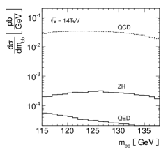
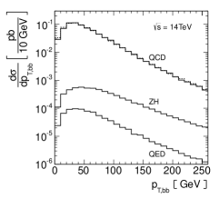
To simplify the MadMax analysis we generate events for the QCD continuum background using the irreducible $Zb\bar{b}$ process. To get a handle on the perturbative accuracy of this simulation we also compute a $Zb\bar{b}$ event sample with up to two hard additional jets, consistently combined between the hard matrix element and the parton shower using Madgraph madgraph with Mlm multi–jet merging mlm . While such an event sample is not formally improved in fixed–order perturbation theory, it should capture the leading effects from large logarithms as well as from initial states opening only in combination with additional jets in the final state zbb_nlo . The difference between the total leading–order $Zb\bar{b}$ rate to the merged prediction implies correction factors around 2.1. For the continuum QCD background the distribution of the merged sample including up to two hard jets is indeed harder than for the fixed–order $Zb\bar{b}$ process. While we use the simpler, fixed–order event sample in our MadMax analysis, we reweight it to the merged $p_{T,bb}$ distribution using the $p_{T,bb}$-dependent correction factor

$$\log\frac{d\sigma_{\text{ME+PS}}}{d\sigma_{\text{LO}}}=0.65+1.1\times 10^{-3}\,p_{T,bb}+4.0\times 10^{-6}\,p_{T,bb}^{2}\;.$$ (7)

The increasing form as a function of $p_{T,bb}$ we limit by fixing the cross section ratio for all values above $p_{T,bb}>350$ GeV to the maximum value, even though the number of events in this phase space is too small to observe any effects from such a cut-off.

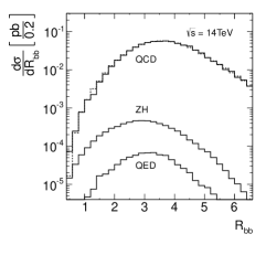
We illustrate the $p_{T,bb}$ distributions for the signal and the backgrounds in the center panel Fig. 1. The $p_{T,H}$ distribution for the signal is slightly less steep than the corresponding background distributions, owing to the gluon parton densities and a general QCD preference for small invariant masses between jets. Nevertheless, the Poisson factor in our statistical analysis will essentially remove the few events with $p_{T,H}>250$ GeV for an integrated luminosity in the $50-100~{}{\rm fb^{-1}}$ range. As a test, we also show the geometric separation of the two $b$-jets in the right panel of Fig. 1. The $p_{T,bb}$-dependent correction perfectly reproduces the multi-jet merged distribution for this observable.

Figure 2: Maximum significance for the $ZH$ signal for slices in the reconstructed $p_{T,bb}$ (left) and the geometric separation of the $b$-jets, $R_{bb}$ (right). We only consider events inside the mass window $m_{bb}=114-138$ GeV. The significance is computed for an integrated luminosity of $50~{}{\rm fb^{-1}}$.

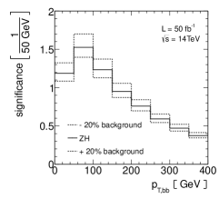
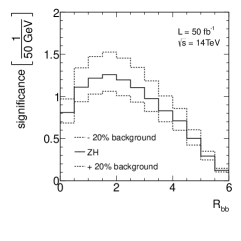
As an estimate of the maximum significance over the entire phase space we obtain $2.7\pm 0.3~{}\sigma$ for an integrated luminosity of $50~{}{\rm fb^{-1}}$. The error bar is given by a $\pm 20\%$ variation in the normalization of the signal rate. The total maximum significance at higher integrated luminosities can be approximately computed by a Gaussian scaling. In the left panel of Fig. 2 we show how this maximum significance is shared between slices of $p_{T,bb}$. The phase space regime best suited to distinguish signal from background events at this limited luminosity is

$$p_{T,H}=50-100~{}{\rm GeV}\;.$$ (8)

Boosted Higgs analyses in the $ZH$ channel indeed significantly reduce the QCD continuum background, but Higgs taggers should be optimized for as low $p_{T,H}$ values as possible. The reason for this finite transverse momentum range is on the one hand that for the background there does not exist a large mass scale in the process, which means that a sizeable $b\bar{b}$ invariant mass has to be generated through a geometric separation, namely $m_{bb}^{2}\simeq 2E_{1}E_{2}(1-\cos\theta)$. In contrast, if we require the $H\to b\bar{b}$ decay to be boosted, the $b$-jets in the signal will move closer together, making it harder for the QCD background to fake the Higgs signal. On the other hand, while we would naively expect higher transverse momenta to carry more and more weight in the analysis, the number of signal events in this range is strongly limited. Asking for $p_{T,bb}>150$ already drives us into a strongly statistics limited phase space regime.

In the right panel of Fig. 2 we show how the maximum significance is composed by slices in the geometric separation $R_{bb}$. This example illustrates how MadMax can be used to analyze the maximum significance distribution in terms of any phase space observable. The separation of the two $b$-tagged jets is crucial for the definition of the fat jet as the starting point of any Higgs tagger. From Fig. 1 it is clear that hardly any signal events lie in the range $R_{bb}\lesssim 1.0$. To optimize a boosted Higgs analysis it appears to be beneficial to extend the fat jet size towards $R_{bb}\sim 2.0$.

Additional effects can still modify the outcome of our study. First, we assume that the detector performance does not depend on the boost of the $b\bar{b}$ system. This is clearly only true up to a certain $p_{T,bb}$ range, where the two bottom jets start overlapping. Second, we assume theory uncertainties to be independent of $p_{T,bb}$. It is not clear if this statement holds for QCD effects, and it is clearly not true in the electroweak sector, once we include electroweak Sudakov logarithms. Finally, we did not actually study dangerous observables, for example, defined in the pre-jet stage of the analysis or at odds with the assumed factorization properties of the signal and background predictions. In that sense MadMax clearly does not deliver a realistic estimate of systematic and theoretical uncertainties. It is merely a first step which allows us to study phase space patterns easily and reliably. For example the question to what degree the estimated uncertainties are realistic and what the effect of shape uncertainties in the background might be will be left to possible further studies.

III Boosted $\mathbf{t\bar{t}H}$ production

The second process for which we want to ask the question where the main distinguishing phase space features exist is $t\bar{t}H$ production with a Higgs decay to $b$-quarks. Two studies indicate that boosted top and Higgs configurations might be promising to extract the signal from the background: for purely hadronic events the buckets methods successfully targets moderate transverse momenta around $p_{T,t}\gtrsim 150$ GeV buckets . For semileptonic top pairs the HEPTopTagger study shows that slightly larger boosts $p_{T,t}\gtrsim 200-250$ GeV can be successfully probed tth . Purely leptonic top pairs have recently been shown to lead to promising results based on a MadWeight study tth_lep . In the semi–leptonic and hadronic cases it is obvious that the boosted kinematics is an excellent way to resolve combinatorial issues tth ; tth_comb . The open question is to what degree the arguments presented in the last section also point to a boosted $t\bar{t}H$ search in terms of the signal and background matrix elements.

To answer this question we will first assume that the continuum $t\bar{t}b\bar{b}$ background is the most relevant issue. For the semileptonic analysis this has been shown, once we require at least three $b$-tags tth . For the purely hadronic channel the removal of the QCD backgrounds is considerably more tedious, but appears to be possible buckets . We follow this study and as a first step require four $b$-tagged jets with an efficiency of 60% each. In addition, we assume a set of global cuts or other ways to reduce the multi–jet backgrounds with a conservatively estimated efficiency around 10% for the $t\bar{t}H$ signal and the irreducible $t\bar{t}b\bar{b}$ background.

To study the combinatorics of the $b$-jets identified as Higgs decay we would have to simulate top decays. However, this is precisely the issue which we want to separate from our significance study over phase space. Therefore, we can assume the top quarks to be fully reconstructed. For hadronic top decays a major part of the buckets buckets and HEPTopTagger studies heptop have been devoted to quantifying the quality of this momentum reconstruction. Moreover, in the absence of additional missing energy from the hard process one hadronic top tag can be combined with an efficient approximate reconstruction of the boosted leptonic top decay leptonic_top . The efficiency of actually reconstructing a hadronic top decay using a top tagger is strongly dependent on the transverse momentum. We roughly estimate it to 33% per top quark, in addition to the branching ratio of 68%. This way we should obtain at least a semi-realistic number for the integrated maximum significance. As mentioned before, such global efficiencies will not affect the main outcome of our study, i.e.  the distribution of the maximum significance over the transverse momentum range of the heavy particles.

For the Higgs decay to bottoms we again include a branching ratio of 58% hdecay . To approximately include detector effects we evaluate the Higgs propagator with a Gaussian width of $\pm 12$ GeV. The mass window of $m_{bb}=114-138$ GeV with a signal efficiency of 68% we carry through the entire analysis, both for the signal and for the background. As discussed in the previous section this ensures that we avoid gluon splitting issues in the background simulation and at the same time allows for side bands in the obvious $m_{bb}$ distribution tth .

Figure 3: Left: $p_{T,bb}$ for signal and backgrounds inside the mass window $m_{bb}=114-138$ GeV. Center and right: transverse momenta of the two tops. For the signal and the QCD background the solid lines approximate the merged results by using the $p_{T}$-dependent correction factors of Eqs.(9) and (10). The merged multi–jet simulation are shown as dotted lines.

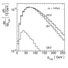
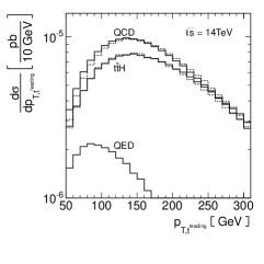
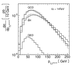
For the $t\bar{t}H$ signal the next-to-leading order corrections are known tth_nlo . Since our study is focused on the phase space structure, we approximately include them by correcting the $p_{T,H}$ distribution to agree with a matched $t\bar{t}H$ plus zero and one jet simulation in the Mlm scheme mlm the same way as we do with the $Zb\bar{b}$ background in Eq.(7). We find a correction factor for the $t\bar{t}H$ signal,

$$\log\frac{d\sigma_{\text{ME+PS}}}{d\sigma_{\text{LO}}}=0.53-2.5\times 10^{-3}\,p_{T,H}+2.0\times 10^{-5}\,p_{T,H}^{2}-3.9\times 10^{-8}\,p_{T,H}^{3}\;.$$ (9)

For a $t\bar{t}b\bar{b}$ background study in the boosted Higgs regime it is absolutely crucial that we correctly simulate the transverse momentum of the $b\bar{b}$ system. While the events entering the MadMax analysis are generated as $t\bar{t}b\bar{b}$ production in Madgraph, we can correct the $p_{T,bb}$ distribution to agree with matched $t\bar{t}b\bar{b}$ plus zero and one jet simulation using

$$\log\frac{d\sigma_{\text{ME+PS}}}{d\sigma_{\text{LO}}}=0.98-6.7\times 10^{-3}\,p_{T,bb}+3.8\times 10^{-5}\,p_{T,bb}^{2}-7.6\times 10^{-8}\,p_{T,bb}^{3}\;.$$ (10)

As for the $ZH$ case we cut off both correction factors using a constant value above $p_{T,bb}=350$ GeV. This reweighting of the differential cross section should account for the leading logarithmic higher–order corrections tth_nlo ; ttbb_nlo , in particular linked to different partons in the initial state. In the left panel of Fig. 3 we show the corresponding distributions, after including the two $p_{T}$-dependent correction factors.

Figure 4: Maximum significance for the $t\bar{t}H$ signal for slices in the reconstructed $p_{T,bb}$ (left), the geometric separation of the two $b$-jets, $R_{bb}$ (center), and the leading top transverse momentum $p_{T,t^{\text{leading}}}$ (right). We only consider events inside the mass window $m_{bb}=114-138$ GeV. The significance is computed for an integrated luminosity of $50~{}{\rm fb^{-1}}$.

For the $t\bar{t}H$ analysis not only the boost of the Higgs candidate, but also the boost of each top is relevant for the analyses tth ; buckets . Therefore, we need to test to what degree the reweighting in Eqs.(9) and (10) affects the top kinematics. In the center and right panels of Fig. 3 we compare the background $p_{T,t}$ distributions for the fully merged event sample with the $p_{T,bb}$-reweighted $t\bar{t}b\bar{b}$ sample. We see that the only phase space region not perfectly described by the $p_{T,bb}$-dependent correction factor is the low-$p_{T}$ range of the two tops. However, the difference is a mere 5%, covered by the theory uncertainty, in a phase space region which will turn out relatively unimportant.

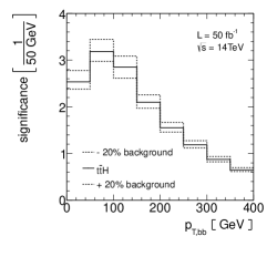
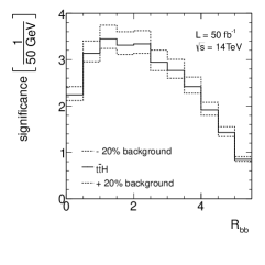
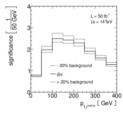
For the set of approximate efficiencies listed above we estimate the maximum significance of the $t\bar{t}H$ to $5.3\pm 0.5~{}\sigma$ for an integrated luminosity of $50~{}{\rm fb^{-1}}$ at a collider energy of 14 TeV. The quoted error bar is again defined by a $\pm 20\%$ variation of the signal rate. Again, values for higher luminosities can be inferred by Gaussian scaling. In Fig.4 we show this maximum significance in slices of the transverse momentum of the reconstructed Higgs system, the separation of the Higgs decay jets, and the transverse momentum of the leading top. For the Higgs boost we find a similar range as for the $ZH$ channel, while the most promising transverse momentum range for the heavier top roughly scales with $m_{t}/m_{H}$,

$$p_{T,H} =\;50-100~{}{\rm GeV}$$

$$p_{T,t} =100-250~{}{\rm GeV}\;.$$ (11)

This result indicates that the requirements for the Higgs tagger bdrs in the $ZH$ and $t\bar{t}H$ analyses are very similar. The only difference between these two channels is that for the $t\bar{t}H$ process the Higgs tagger has to be adapted to higher jet multiplicities, as done in Ref. tth . For the top tagger it is crucial that we gain access to transverse momenta well below $p_{T,t}=300$ GeV, ruling out most of the currently available analysis tools optimized for heavy $t\bar{t}$ resonance searches top_tagger .

IV Conclusions

In this paper we have introduced MadMax as a novel approach to studying the composition of a signal significance in terms of the signal and background phase space. It allows us to determine those phase regions which are best suited for the extraction of a signal process from irreducible backgrounds in an efficient and mathematically well–defined manner orig .

Relying on MadMax we have studied the two Higgs search channels involving a hadronic $H\to b\bar{b}$ decay, namely associated $ZH$ and $t\bar{t}H$ production. In both cases the central question is to what degree boosted Higgs configurations benefit the signal extraction and what range in transverse Higgs momenta we should target. Unlike in the original study orig , we specifically did not focus on predicting the integrated maximum significance for each of these processes, so detector effects as well as global efficiencies are only adjusted to obtain a semi-realistic number.

For the $ZH$ channel we find that for integrated luminosities in the $50-100~{}{\rm fb^{-1}}$ range the most promising phase space regime is around or below $p_{T,H}=100$ GeV, challenging the development of Higgs taggers. For the $t\bar{t}H$ analysis the first reason to rely on boosted top and Higgs decay topologies is the otherwise overwhelming combinatorial background. In this study we estimated the additional motivation for using these topologies based on the matrix element structure of the signal and the irreducible background. The most promising range in the transverse momentum of the reconstructed Higgs boson again came out as $p_{T,H}=50-100$ GeV, indicating that the same Higgs tagger should suit both analyses. To include as many of the relevant signal events as possible the size of the fat jet could be extended towards $R_{bb}\sim 2$, if possible. For the transverse momentum of the leading top quark the significance is mostly collected for $p_{T,t}=100-250$ GeV, seriously challenging the development of hadronic top taggers.

We note that MadMax is an automized tool which can be used in the Madgraph5 framework to produce multi–dimensional differential distributions adding to the maximum significance in any kinematic observable. Some of its current limitations, like the focus on irreducible backgrounds can be overcome easily. Likewise, simple transfer functions can be included in a straightforward manner. Once these effects are taken into account, we should be able to also give a more reliable estimate of the integrated maximum significance for a signal–background combination.

Acknowledgments

First of all, we would like to thank Kyle Cranmer for supporting this extension of the original work of Ref.orig . PS would like to thank the IMPRS Precision studies of fundamental symmetries for their never–ending support. TP would like to thank the CCPP at New York University for their hospitality in a crucial phase of this paper. DW is grateful to the University of Pittsburgh and to Ayres Freitas for supporting him while writing this paper, as well as to Jan Pawlowski for agreeing to co-referee his rather technical thesis. Finally, all of us would like to thank Fabio Maltoni for suggesting the name MadMax.

Appendix A MadMax in Madgraph

To understand how MadMax works together with Madgraph5 madgraph we first describe some of the main Madgraph features. To construct the log–likelihood map of Eq.(3) we need the squared matrix elements for the signal and background, which Madgraph5 computes using a modified version of Helas helas . These matrix elements are integrated using the so-called single diagram enhanced method madevent to account for the propagator structure. A good example process is $pp\to\mu^{+}\mu^{-}$, where we compute the cross–section via

$$\sigma_{\text{tot}}=\int dx_{1}\,dx_{2}\,d\text{LIPS}\;f_{p}(x_{1},\mu_{F})\,f_{p}(x_{2},\mu_{F})\;\left|\sum\limits_{n}\mathcal{M}_{n}\right|^{2}\;.$$ (12)

The phase space is described by a random number vector $r$ and transforms the integral into a sum over phase space cells $\Delta r$. The parton densities are evaluated together with the matrix elements, so in the following we implicitly include them in $\mathcal{M}$. We can improve the convergence if we know the leading behavior of the individual matrix elements,

$$\sigma_{\text{tot}}=\sum\limits_{r}\;\Delta r\;\left|\sum\limits_{n}\mathcal{M}_{n}(r)\right|^{2}=\sum\limits_{r,i}\Delta r\,\frac{\left|\mathcal{M}_{i}(r)\right|^{2}}{\sum\limits_{n}\left|\mathcal{M}_{n}(r)\right|^{2}}\times\left|\sum\limits_{n}\mathcal{M}_{n}(r)\right|^{2}\;.$$ (13)

The optimized phase space mapping is different for each diagram $i$. For our example we optimize for a $1/s$ scaling in the photon exchange and for a Breit–Wigner propagator in the $Z$ exchange. In addition, the sum over diagrams is decomposed into incoherent partial sums for different incoming partons, so an additional weight accounts for the parton densities,

$$\sigma_{\text{tot}}=\sum\limits_{r,i,p}\Delta r\,\frac{\left|\mathcal{M}_{i_{p}}(r)\right|^{2}}{\sum\limits_{n_{p}}\left|\mathcal{M}_{n_{p}}(r)\right|^{2}}\times\left|\sum\limits_{n_{p}}\mathcal{M}_{n_{p}}(r)\right|^{2}\times\omega_{p}^{\text{pdf}}(r)\;.$$ (14)

In this framework MadMax computes the maximum significance using a log–likelihood ratio integration. It starts from the single event likelihood for signal and background. For each phase space point we need to know simultaneously

$$d\sigma_{s}(r) =\left|\sum\limits_{n_{s}}\mathcal{M}_{n_{s}}(r)\right|^{2}\qquad\qquad\qquad d\sigma_{b}(r)=\left|\sum\limits_{n_{b}}\mathcal{M}_{n_{b}}(r)\right|^{2}$$

$$q(r) =-\sigma_{\text{tot,s}}\,\mathcal{L}+\log\left(1+\frac{d\sigma_{s}(r)}{d\sigma_{b}(r)}\right)\;,$$ (15)

as quoted in Eq.(3). From the logarithm in the log–likelihood ratio it is clear that the we cannot use the single enhanced diagram method. Instead, we will use a modified version closer to the original proposal madevent : let us assume our signal process consists of $a_{s}\in[1,\ldots,n_{s}]$ sub-processes, with different partons in the initial and final state. Each sub-process will be computed using $i_{a_{s}}\in[1,\ldots,n_{a_{s}}]$ matrix elements. The same is true for the background, namely $a_{b}\in[1,\ldots,n_{b}]$ subprocesses with $i_{a_{b}}\in[1,\ldots,n_{a_{b}}]$ matrix elements. Any function $f(r)$ we can construct using the basis elements

$$\frac{\left|\mathcal{M}_{i}(r)\right|^{2}}{\sum\limits_{\begin{subarray}{c}a_{s},i_{a_{s}}\\ a_{b},i_{a_{b}}\end{subarray}}\left|\mathcal{M}_{n}(r)\right|^{2}}\times f(r)\;.$$ (16)

In this basis we can integrate all signal and background rates. Furthermore, the points $q(r)$ defining the single event probability have the correct weight as well. The only remaining issue is that events in Madgraph5 are usually computed with a dynamical factorization and renormalization scale choice. In MadMax we add, divide, and combine matrix elements from signal as well as background processes. In the current implementation of MadMax we use fixed factorization and renormalization scales, to simplify the interface to Madgraph5. The implementation of a general scale choice would be straightforward.

Figure 5: Example MadMax output for the $ZH$ channel. We give the computed signal and background cross–sections as well as the corresponding standard Madgraph results. In addition, we give all constant efficiencies and $K$-factors included in the statistical analysis.

We test and validate our implementation in two ways. First, we have compared our findings for weak–boson–fusion Higgs production with a Higgs decay to muons with the original results orig . Second, for each set of signal and background processes we can compare our signal and background cross–sections with the Madgraph5 results obtained in parallel, an example output is shown in Fig. 5. The numbers always agree within the numerical uncertainties. An extensive validation study as well as more information on the implementation of MadMax can be found in Ref. daniel .

References

- (1) K. Cranmer and T. Plehn, Eur. Phys. J. C 51, 415 (2007).
- (2) M. Klute, R. Lafaye, T. Plehn, M. Rauch and D. Zerwas, Europhys. Lett. 101, 51001 (2013).
- (3) J. M. Butterworth, A. R. Davison, M. Rubin, G. P. Salam, Phys. Rev. Lett. 100, 242001 (2008); ATLAS note, ATL-PHYS-PUB-2009-088.
- (4) T. Plehn, G. P. Salam and M. Spannowsky, Phys. Rev. Lett. 104, 111801 (2010).
- (5) M. R. Buckley, T. Plehn and M. Takeuchi, JHEP 1308, 086 (2013); M. R. Buckley, T. Plehn, T. Schell and M. Takeuchi, arXiv:1310.6034 [hep-ph].
- (6) for recent overviews see e.g. A. Altheimer, S. Arora, L. Asquith, G. Brooijmans, J. Butterworth, M. Campanelli, B. Chapleau and A. E. Cholakian et al., J. Phys. G 39, 063001 (2012); T. Plehn and M. Spannowsky, J. Phys. G 39, 083001 (2012).
- (7) D. E. Soper and M. Spannowsky, Phys. Rev. D 84, 074002 (2011); D. E. Soper and M. Spannowsky, Phys. Rev. D 87, no. 5, 054012 (2013).
- (8) J. Alwall, P. Demin, S. de Visscher, R. Frederix, M. Herquet, F. Maltoni, T. Plehn and D. L. Rainwater et al., JHEP 0709, 028 (2007); J. Alwall, M. Herquet, F. Maltoni, O. Mattelaer and T. Stelzer, JHEP 1106, 128 (2011).
- (9) for a proof and corresponding definitions, see e.g. J. Stuart, A. Ord and S. Arnold, Kendall’s Advanced Theory of Statistics, Vol 2A (6th Ed.) (Oxford University Press, New York, 1994); for a pedagogical introduction in the context of high-energy physics, see A. Read, in ‘1st Workshop on Confidence Limits’, CERN Report No. CERN-2000-005 (2000).
- (10) for some early examples see e.g. K. Kondo, J. Phys. Soc. Jap. 57, 4126 (1988); D. Atwood and A. Soni, Phys. Rev. D 45, 2405 (1992); M. Diehl and O. Nachtmann, Eur. Phys. J. C 1, 177 (1998).
- (11) see some early examples see e.g. V. M. Abazov et al. [D0 Collaboration], Phys. Lett. B 617, 1 (2005); A. Abulencia et al. [CDF Collaboration], Phys. Rev. D73, 092002 (2006); V.M Abazov et. al. [D0 Collaboration], Nature 429, 638 (2004).
- (12) P. Artoisenet, V. Lemaitre, F. Maltoni and O. Mattelaer, JHEP 1012, 068 (2010).
- (13) H. Hu and J. Nielsen, in ‘1st Workshop on Confidence Limits’, CERN 2000-005 (2000) [arXiv:physics/9906010].
- (14) K. Cranmer, LEPStats4LHC, https://plone4.fnal.gov/P0/phystat/packages/0703002
- (15) D. Lopez-Val, T. Plehn and M. Rauch, JHEP 1310, 134 (2013).
- (16) for a pedagogical introduction see e.g. T. Plehn, Lect. Notes Phys. 844, 1 (2012); [arXiv:0910.4182 [hep-ph]].
- (17) T. Plehn, M. Spannowsky, M. Takeuchi and D. Zerwas, JHEP 1010, 078 (2010); T. Plehn, M. Spannowsky and M. Takeuchi, Phys. Rev. D 85, 034029 (2012); G. Aad et al. [ATLAS Collaboration], JHEP 1301, 116 (2013); http://www.physi.uni-heidelberg.de//Publications/Kasieczka-Doktor.pdf
- (18) A. Djouadi, J. Kalinowski and M. Spira, Comput. Phys. Commun. 108, 56 (1998).
- (19) O. Brein, A. Djouadi and R. Harlander, Phys. Lett. B 579, 149 (2004); S. Dawson, T. Han, W. K. Lai, A. K. Leibovich and I. Lewis, Phys. Rev. D 86, 074007 (2012).
- (20) M. L. Mangano, M. Moretti, F. Piccinini and M. Treccani, JHEP 0701, 013 (2007).
- (21) J. M. Campbell and R. K. Ellis, Phys. Rev. D 62, 114012 (2000); F. Febres Cordero, L. Reina and D. Wackeroth, Phys. Rev. D 80, 034015 (2009).
- (22) P. Artoisenet, P. de Aquino, F. Maltoni and O. Mattelaer, arXiv:1304.6414 [hep-ph].
- (23) J. Cammin and M. Schumacher, ATL-PHYS-2003-024; for an experimental update see e.g. S. Allwood-Spiers, ATL-PHYS-PROC-2011-280.
- (24) J. Thaler and L. -T. Wang, JHEP 0807, 092 (2008); K. Rehermann and B. Tweedie, JHEP 1103, 059 (2011); T. Plehn, M. Spannowsky and M. Takeuchi, JHEP 1105, 135 (2011).
- (25) W. Beenakker, S. Dittmaier, M. Krämer, B. Plümper, M. Spira and P. M. Zerwas, Nucl. Phys. B 653, 151 (2003); S. Dawson, C. Jackson, L. H. Orr, L. Reina and D. Wackeroth, Phys. Rev. D 68, 034022 (2003).
- (26) A. Bredenstein, A. Denner, S. Dittmaier and S. Pozzorini, Phys. Rev. Lett. 103, 012002 (2009); A. Bredenstein, A. Denner, S. Dittmaier and S. Pozzorini, JHEP 1003, 021 (2010); G. Bevilacqua, M. Czakon, C. G. Papadopoulos, R. Pittau and M. Worek, JHEP 0909, 109 (2009).
- (27) H. Murayama, I. Watanabe and K. Hagiwara, KEK-91-11, http://madgraph.kek.jp/~kanzaki/Tutorial/helas.pdf
- (28) F. Maltoni and T. Stelzer, JHEP 0302, 027 (2003).
- (29) D. Wiegand, master thesis (2013), http://www.thphys.uni-heidelberg.de/~plehn/includes/theses/wiegand.pdf