A New Dynamic Pricing Method Based on
Convex Hull Pricing

Abstract

This paper presents a new dynamic pricing model (a.k.a. real-time pricing) that reflects startup costs of generators. Dynamic pricing, which is a method to control demand by pricing electricity at hourly (or more often) intervals, has been studied by many researchers. They assume that the cost functions of suppliers are convex, although they may be nonconvex because of the startup costs of generators in practice. We provide a dynamic pricing model that takes into account such cost functions within the settings of unit commitment problems (UCPs). Our model gives convex hull price (CHP), which has not been used in the context of dynamic pricing, though it is known that the CHP minimizes the uplift payment which is disadvantageous to suppliers for a given demand. In addition, we apply an iterative algorithm based on the subgradient method to solve our model. Numerical experiments show the efficiency of our model on reducing uplift payments. The prices determined by our algorithm give sufficiently small uplift payments in a realistic computational time.

I Introduction

Dynamic pricing (a.k.a. real-time pricing) is a method of invoking a response in demand by pricing electricity at hourly (or more often) intervals. There are many studies about dynamic pricing. For example, Roozbehani et al. [2] proposed a nonlinear control model in a real-time market, in which prices are updated on moment-to-moment basis. They focused on the stability of the market, and analyzed stabilizing effects of their model by using volatility measures of the prices. On the other hand, Miyano and Namerikawa [3] proposed a dynamic pricing model in a day-ahead market, in which a market operator sets next day’s hourly (or more often) prices. Their price is given by the Lagrange multiplier of a social welfare maximization problem. They studied an algorithm based on a steepest descent method to control the load levels, and showed its convergence. Their numerical results show the efficiency of their algorithm.

These studies assume that the cost functions of suppliers are convex, although they may be nonconvex because of the startup costs of generators in practice (in fact, there are many studies that deal such cost functions within the settings of unit commitment problems (UCPs)). Thus, these models do not fully reflect the startup costs to the prices, and would be disadvantageous to the suppliers. One of the measures showing the disadvantages is the uplift payment which is the gap between the suppliers’ optimal profit and actual profit. If the cost functions are truly convex, a marginal cost price can make the uplift payments zero. However, if not, none of pricing models may make the uplift payments zero. The uplift payments for owners of many generators tend to be relatively small and can often be ignored. However, this may not be true for small producers since startup costs occupy a large portion of the total cost of electricity generation.

Recently, under the assumption that the demand is given (i.e., out of the context of the dynamic pricing), several pricing models [4, 5, 6, 7, 8] have been proposed in order to reduce the uplift payments. The most successful pricing model is the convex hull pricing (CHP) model (a.k.a. extended locational marginal pricing model) proposed by Gribik et al. [5]. The authors theoretically showed that the CHP is given by the Lagrange multiplier for the UCP, and the CHP minimizes the uplift payment for a given demand. Many researchers have studied algorithms to calculate the CHP, e.g., [9, 10]. However, they have not been used in the context of dynamic pricing.

This paper presents a new dynamic pricing model based on the CHP. First, we formulate a social welfare maximization problem, which maximizes the sum of the consumers’ utility and the suppliers’ profit under the condition that supply and demand are equal, with nonconvex cost functions of the suppliers within the settings of the UCP. Then we applied a CHP approach, which is invented for the UCP, to the social welfare maximization problem; our model takes into account both the startup costs and dynamic demand. We prove that the CHP is given by a solution of its dual problem, i.e., the Lagrange multiplier for the social welfare maximization problem. This implies that our price minimizes the uplift payment for the equilibrium demand. Since our pricing model has a nonsmooth objective function including 0-1 integer variables, it is difficult to be solved by exact optimization algorithms. Thus we provide an approximate pricing algorithm based on the subgradient method. Numerical results show that our pricing model leads to smaller uplift payments compared with standard dynamic pricing models. Moreover, our algorithm achieves sufficiently small uplift payments in a realistic number of iterations and computational time.

The rest of this paper is organized as follows. Section II presents the setting of a dynamic electricity market. Section III presents the definition of the UCP and the CHP. Section IV introduces a new dynamic pricing model based on a social welfare maximization that includes the UCP. In addition, we theoretically show that our pricing model leads to the CHPs. We also provide a pricing algorithm based on the subgradient method. Numerical results are reported in Section V. We give conclusions and list possible directions for research in Section VI.

In what follows, we denote column vectors in boldface, e.g., $\bm{x}\in\mathbb{R}^{n}$ whose $i$-th element is $x_{i}\in\mathbb{R}~{}(i=1,2,\dots,n)$.

II Market Model

We will begin by describing the electricity market model and existing pricing models. Assumptions in this section are made along the lines of [2, 3]. There are three kinds of participants in an electricity market: consumers, suppliers, and an independent system operator (ISO). The suppliers (or consumers) decide their electric power production (or consumption) so as to maximize their profit (or utility, respectively) at a given electricity price. The ISO is a non-profit institution that is independent of the suppliers and the consumers. The ISO makes hourly (or more often) pricing decisions to balance supply and demand. We assume that resistive losses can be ignored. Further, there are no line capacity constraints and reserve capacity constraints.

II-A Supply and demand models

To make our model simple, we suppose a single representative supplier (or consumer) whose response represents the macro behavior of all suppliers (or consumers), and focus on a single-period model that deals with each period independently (i.e., a model with that does not take into account dynamical changes). Our model and algorithm can be extended to a multi-agent and multi-period model, as is shown in [4]. Let $u:~{}[0,\infty)\rightarrow[0,\infty)$ be the utility function of the representative consumer, which represents the dollar value of consuming electricity. Let $v:~{}[0,\infty)\rightarrow[0,\infty]$ be the cost function of the representative supplier, which represents the dollar cost of producing electricity. For a given price $p>0$, the consumer (or supplier) makes their demand $d(p)$ (or supply $s(p)$) to maximize their utility (or profit, respectively), i.e.,

$$d(p) \in\mathop{\rm arg~{}max}\limits_{d\geq 0}~{}u(d)-pd,$$ (1)

$$s(p) \in\mathop{\rm arg~{}max}\limits_{y\geq 0}~{}py-v(y).$$ (2)

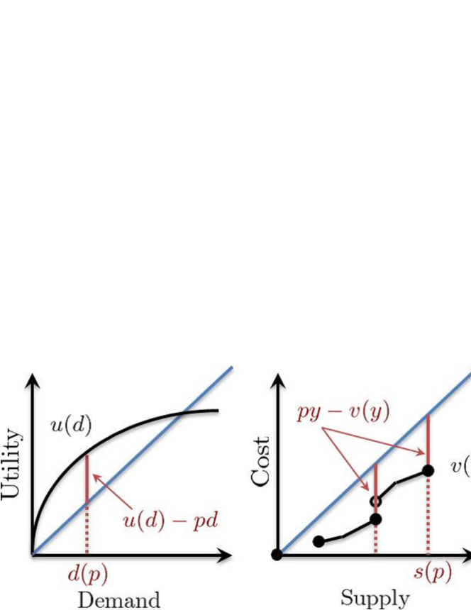
Figure 1: Illustration of supply and demand models. The left panel illustrates the consumer’s problem (1), and the right panel illustrates the supplier’s problem (2). The vertical solid lines represent optimal utility and profit for each agent. In this case, the supplier has two optimal solutions. The cost function $v$ in the right panel is nonconvex and discontinuous. We deal with such cost functions in this paper.

A conceptual illustration is given in Fig. 1. The existing works [2, 3] assume the following assumption:

Assumption 1 ([2, 3]).

The utility function $u$ is class-$\mathcal{C}^{2}$, monotonically increasing, and strictly concave on $[0,\infty)$. The cost function $v$ is class-$\mathcal{C}^{2}$, monotonically increasing, and strictly convex on $[0,\infty)$.

Note that if there exist a solution of (1) (or (2)), it is unique under Assumption 1.

II-B Pricing model

The ISO is a non-profit institution and independent from the consumer and the supplier. The objective of the ISO is to manage the electricity market, especially, to balance demand and supply. In the electricity market, neither the consumer and the supplier do not bid. Thus, the ISO should match the levels of demand $d(p)$ and supply $s(p)$ by making an appropriate pricing decision $p$. Here, it is natural to assume that the utility function $u$ of the consumer is unknown to the ISO, while the cost function $v$ of the supplier is not necessarily known to the ISO. Accordingly, an electricity price $p$ is determined through the following procedure:

Algorithm 1.

1. The ISO sets the initial price $p^{0}$, and sends it to the consumer and supplier. $k\leftarrow 0$.

2. The consumer and supplier respectively determine the demand $d(p^{k})$ and the supply $s(p^{k})$, and send them to the ISO.

3. If there is a gap between the demand $d(p^{k})$ and supply $s(p^{k})$, the ISO reassign a new price $p^{k+1}$ to manage the balance of supply and demand, and send it to the consumer and supplier again. $k\leftarrow k+1$.

4. Step 2 and 3 are repeated.

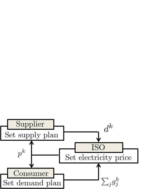
Figure 2: Schematic views of the electricity market model.

Miyano and Namerikawa [3] proposed a pricing model based on social welfare maximization problem with the supply-demand balance constraint. The social welfare is represented as the sum of the consumer’s utility and supplier’s profit:

$$\{u(d)-pd\}+\{py-v(y)\}.$$ (3)

Since we assumed that the resistive losses can be ignored, the supply-demand balance constraint is $d=y$. Consequently, we obtain the following social welfare maximization problem:

$$\max_{d\geq 0,y\geq 0}u(d)-v(y)\quad\text{s.t.}\quad d=y.$$ (4)

Or more simply,

$$\max_{d\geq 0}~{}u(d)-v(d).$$ (5)

However, the ISO cannot solve (4) (or (5)) directly since the utility function $u$ is unknown to the ISO. Therefore, the following partial Lagrangian dual problem of (4) is alternatively considered in [3]:

$$\min_{\lambda}~{}\varphi(\lambda),$$ (6)

where

$$\varphi(\lambda) =\max_{d\geq 0,y\geq 0}u(d)-v(y)+\lambda(y-d)$$

$$=\max_{d\geq 0}\{u(d)-\lambda d\}+\max_{y\geq 0}\{\lambda y-v(y)\}.$$ (7)

Since the maximization problems in (7) correspond to (1) and (2), the ISO can make the consumer and supplier solve them by sending $\lambda$ as a price. This mechanism allows the ISO to solve (6) by using the steepest descent method (See [3] for details). The following lemma is well known (e.g. [3, 11]).

Lemma 1.

Suppose that $(d^{*},y^{*})$ is an optimal solution of (4), and $\lambda^{*}$ is an optimal solution of (6). If Assumption 1 is satisfied, $d^{*}=d(\lambda^{*})$ and $y^{*}=s(\lambda^{*})$ hold.

$\lambda^{*}$ is called the Lagrange multiplier for (4). Lemma 1 states that the demand $d(\lambda^{*})$ and the supply $s(\lambda^{*})$ maximize the social welfare (3), and therefore, the Lagrange multiplier $\lambda^{*}$ can be regarded as an optimal price.

These results hold under the assumption that the cost function $v$ is convex. Here, we consider an electricity market model with a nonconvex cost function within the setting of the unit commitment problem (UCP) and provide an efficient pricing model for it.

III Convex hull pricing model

In this section, we will introduce the convex hull pricing (CHP) model (a.k.a. extended locational marginal pricing model) proposed by Gribik et al. [5]. Note that the models in this section do not take into account dynamic demand; We assume that the demand is given.

III-A Unit commitment problem

First, we consider the supplier’s cost function.

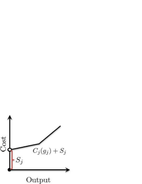
Figure 3: Example of a cost function of generator $j$. $S_{j}$ denotes the startup cost and $C_{j}(g_{j})$ denotes the lower semicontinuous variable cost for an output $g_{j}$.

We assume that the supplier has several types of generators that might have different variable cost functions and startup costs as shown in Fig. 3. The supplier would like to minimize the generating cost for a given demand $y$. Then, the cost function $v:[0,\infty)\rightarrow[0,\infty]$ for the supplier can be represented as the optimal value of the following optimization problem:

$$v(y):=\left|\begin{aligned} \inf_{\bm{g},\bm{z}}~{}&{\textstyle\sum_{j}}C_{j}(g_{j})+{\textstyle\sum_{j}}S_{j}z_{j}\\ \text{s.t. }~{}&{\textstyle\sum_{j}}g_{j}=y\\ &m_{j}z_{j}\leq g_{j}\leq M_{j}z_{j},\quad z_{j}\in\{0,1\},~{}\forall j,\end{aligned}\right.$$ (8)

where $C_{j}(g_{j})$ is a lower semicontinuous generating cost function for an output $g_{j}$; $S_{j}$ denotes the startup cost; $m_{j}$ and $M_{j}$ denote the minimum and maximum outputs; and $z_{j}$ represents a decision to commit generator $j$. Problem (8) is called a unit commitment problem (UCP). The optimal value function $v$ of the UCP is characterized by lower semicontinuity, and it may be nonconvex and discontinuous.

III-B Convex hull price

A number of studies have proposed pricing models in the settings of UCP. Some of them (e.g. [4, 5, 6, 7]) have tried to reduce the uplift payment which is defined as follow.

Definition 1 (Uplift payment).

Suppose that a demand $y$ is given. The uplift payment $\Pi(p;y)$ for a price $p$ is defined as follows:

$$\Pi(p;y):=\sup_{x}\{px-v(x)\}-\{py-v(y)\}.$$ (9)

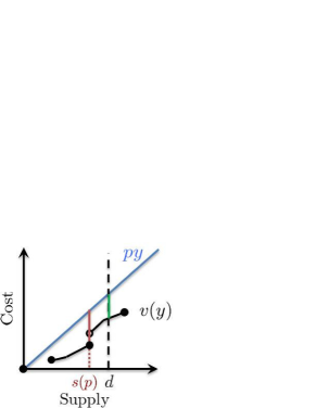
Figure 4: Illustration of the uplift payment. In this picture, $py$ represents net sales. The margin between $py$ and $v(y)$ represents the profit for the supplier. In this case, the optimal profit for the supplier is obtained at $s(p)$. However, demand $d$ is given and the supplier has to supply $d$. Thus, the actual profit for the supplier is obtained at $d$. The gap between the optimal profit and the actual profit is called the uplift payment. It is formulated as (9).

A conceptual illustration is given in Fig. 4. The first term of (9) represents the maximum profit for the supplier, that is realizable under a price $p$. The second term of (9) represents the actual profit for the supplier under a price $p$ and the given demand $y$. The uplift payment can be regarded as a measure of disadvantage for the supplier, or as a cost for the ISO to incentive the supplier to supply the given demand $y$ under the price $p$. Therefore, it is natural to find the price that minimizes the uplift payment.

Such a price can be obtained by the convex hull pricing (CHP) model (a.k.a. extended locational marginal pricing model) proposed by Gribik et al. [5]. Before introducing the CHP, we define the convex hull of the cost function $v(y)$:

Definition 2 (Convex hull of the cost function $v$).

The convex hull $v^{h}$ of the cost function $v$ is defined as

$$v^{h}(y):=\inf_{\mu}\{\mu\mid(y,\mu)\in\text{conv}(\text{epi}(v))\},$$

where $conv(A)$ is the convex hull of a set $A$, and $epi(v)$ denotes the epigraph of $v$.

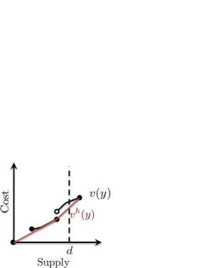
Figure 5: Illustration of the convex hull $v^{h}$ of the cost function $v$. The CHP model uses the subgradient of $v^{h}$ at the given demand $d$ as a price $p^{h}$.

We illustrate the convex hull $v^{h}$ of the cost function $v$ in Fig. 5. The convex hull $v^{h}$ can be seen as the largest convex function that is bounded above by $v$ at any point in its domain. In addition, it is known that $v^{h}$ is coincide with biconjugate (i.e., convex conjugate of convex conjugate) of $v$, if $v$ is lower semicontinuous (see [12]). Note that $v^{h}$ may be a nonsmooth function. Now, we can define the CHP.

Definition 3 (Convex hull price).

The convex hull price $p^{h}$ is defined as the subgradient of the convex hull $v^{h}$ of the cost function $v$ at a given demand $y$ , i.e.,

$$p^{h}\in\partial v^{h}(y).$$

It is difficult to calculate the CHP according to the definition because the explicit function form of $v(\cdot)$ and its convex hull $v^{h}(\cdot)$ are generally too complicated to compute. To address this issue, Gribik et al. investigated the following important properties of the CHP in connection with duality theory.

Proposition 1 ([5]).

Suppose that $\lambda^{*}$ be an optimal solution of the following partial Lagrangian dual problem of (8):

$$\max_{\lambda}\left|\begin{aligned} \min_{\bm{g},\bm{z}}~{}&{\textstyle\sum_{j}}C_{j}(g_{j})+{\textstyle\sum_{j}}S_{j}z_{j}+\lambda(y-{\textstyle\sum_{j}}g_{j})\\ \text{s.t. }~{}&m_{j}z_{j}\leq g_{j}\leq M_{j}z_{j},\quad z_{j}\in\{0,1\},~{}\forall j.\end{aligned}\right.$$ (10)

Then, $\lambda^{*}$ is a convex hull price, i.e.,

$$\lambda^{*}\in\partial v^{h}(y).$$

Moreover, $\lambda^{*}$ minimizes the uplift payment $\Pi(\cdot;y)$, i.e.,

$$\lambda^{*}\in\mathop{\rm arg~{}min}\limits_{p\geq 0}~{}\Pi(p;y).$$

Proposition 1 states that the Lagrangian multiplier for (8) gives the CHP, and the CHP is the best price in the sense of reducing the uplift payment $\Pi(\cdot;y)$. Many researcher have studied algorithms for (10), e.g., [9, 10]. However, there still remains a difficulty to solve a mixed integer programming problem in (10).

IV Pricing Model and Algorithm

In this section, we present a new dynamic pricing model and algorithm that deals with the nonconvex cost function $v$ of (8). Here, we assume that the consumer’s utility function $u$ is concave, non-decreasing, $\lim_{d\rightarrow 0}\dot{u}(d)=0$.

IV-A Pricing model

By adding $v$ of (8) to (4), we derive a new social welfare maximization problem as follows:

$$\max_{\bm{g},\bm{z},d}~{} u(d)-\left\{{\textstyle\sum_{j}}C_{j}(g_{j})+{\textstyle\sum_{j}}S_{j}z_{j}\right\}$$

s.t. $${\textstyle\sum_{j}}g_{j}=d,\quad d\geq 0$$ (11)

$$z_{j}m_{j}\leq g_{j}\leq z_{j}M_{j},\quad z_{j}\in\{0,1\}.\quad\forall j,$$

Since the ISO does not know the utility function $u$, it cannot solve (11). Therefore, we alternatively consider a partial Lagrangian dual problem of (11). For notational simplicity, let $X$ denotes the feasible set for outputs $\bm{g}$ and commitment decisions $\bm{z}$, i.e.,

$$X:=\{(\bm{g},\bm{z})~{}|~{}m_{j}z_{j}\leq g_{j}\leq M_{j}z_{j},~{}z_{j}\in\{0,1\},\forall j\}.$$

The partial Lagrangian dual problem of (11) is formulated by adding $v$ of the UCP (8) to (6) as follows:

$$\min_{\lambda}~{}\varphi(\lambda),$$ (12)

where

$$\varphi(\lambda): =\max_{d\geq 0}\{u(d)-\lambda d\}$$

$$~{}~{}~{}+\max_{(\bm{g},\bm{z})\in X}\left\{\lambda{\textstyle\sum_{j}}g_{j}-{\left\{{\textstyle\sum_{j}}C_{j}(g_{j})+{\textstyle\sum_{j}}S_{j}z_{j}\right\}}\right\}.$$ (13)

The objective function $\varphi$ may be nonsmooth because of the nonsmoothness of the cost function $v$. Note that the problems (11) and (12) take into account price-sensitive demands. Hence they are different from existing CHP models such as those in [5, 9, 10]. Now we have reached the following result.

Proposition 2.

The following statements hold:

1. The partial Lagrangian dual problem (12) has an optimal solution $(\lambda^{*},\bm{g}^{*},\bm{z}^{*},d^{*})$.

2. The problem (12) is equivalent to

   $$\max_{d\geq 0}~{}u(d)-v^{h}(d),$$

3. $\lambda^{*}$ is a convex hull price, i.e.,

   $$\lambda^{*}\in\partial v^{h}(d^{*}).$$

Proof.

The idea behind the proof of 1) is to use the general version of Weierstrass’ Theorem [12], which states that $\varphi$ has a minimum point if $\varphi$ is a closed proper function and has a nonempty and bounded level set. From duality theory it is known that $\varphi$ is lower semicontinuous, and this guarantees the closedness of $\varphi$. For all $\lambda<0$, $\varphi(\lambda)=\infty$ holds since the first term in (13) is infinite, $\infty$. For all $\lambda\geq 0$, the first term in (13) is finite, and an optimal solution exists. The second term in (13) is also finite, and an optimal solution exists because of the compactness of $X$. Thus, if $\lambda^{*}$ exists, $\lambda^{*}$ is a nonnegative number and $(\bm{g}^{*},\bm{z}^{*},d^{*})$ also exists (This implies that $d\leq\sum_{j}g_{j}$ is an effective constraint). Let us choose $\gamma\in\mathbb{R}$ so that the level set $L=\{\lambda~{}|~{}\varphi(\lambda)\leq\gamma\}\in(0,\infty)$ is non-empty. From (13), we have

$$\varphi(\lambda)\geq u(0)+\lambda{\textstyle\sum_{j}}M_{j}-({\textstyle\sum_{j}}C_{j}(M_{j})+{\textstyle\sum_{j}}S_{j})$$

for any $\lambda$. The right-hand side of the inequality is derived by setting $d=0$, $g_{j}=M_{j}$, and $z_{j}=1$ to (13). There exists a sufficiently large $\hat{\lambda}>0$ such that $\varphi(\hat{\lambda})>\gamma$. Hence, $L$ is bounded, and the conditions on the existence of a minimum point of $\varphi$ are satisfied.

The remaining parts can be obtained by mimicking the argument in [5]. The second term in (13) is written as

$$\max_{\eta,(\bm{g},\bm{z})\in X}\left\{\lambda\eta-{\left\{{\textstyle\sum_{j}}C_{j}(g_{j})+{\textstyle\sum_{j}}S_{j}z_{j}\right\}}~{}|~{}\eta={\textstyle\sum_{j}}g_{j}\right\}$$

$$=\max_{\eta}\{\lambda\eta-v(\eta)\}=v^{c}(\lambda),$$

where $v^{c}$ is the convex conjugate function of $v$. Problem (12) can be expressed as

$$\min_{\lambda}\varphi(\lambda) =\min_{\lambda}\max_{d\geq 0}\{u(d)-\lambda d+v^{c}(\lambda)\}$$

$$=\max_{d\geq 0}\min_{\lambda}\{u(d)-\lambda d+v^{c}(\lambda)\}$$

$$=\max_{d\geq 0}\{u(d)-v^{cc}(d)\},$$

where $v^{cc}$ is the biconjugate function of $v$, i.e., the convex conjugate function of $v^{c}$. The second equality holds from [12, Prop. 2.6.4]. To prove 3), we obtain the following result for all $d\geq 0$:

$$v^{cc}(d) =\sup_{\lambda}\{d\lambda-v^{c}(\lambda)\}$$

$$\geq d\lambda^{*}-v^{c}(\lambda^{*})$$

$$=d\lambda^{*}-v^{c}(\lambda^{*})+\lambda^{*}d^{*}-\lambda^{*}d^{*}$$

$$=v^{cc}(d^{*})+\lambda^{*}(d-d^{*}).$$

This implies that $\lambda^{*}$ is a subgradient of $v^{cc}$ at $d^{*}$. Since $v^{cc}=v^{h}$ holds (see [12]), this completes the proof. ∎

Proposition 2 states that the Lagrange multiplier $\lambda^{*}$ for the social welfare maximization problem (11) gives a CHP. This implies that $\lambda^{*}$ minimizes the uplift payment at the equilibrium demand $d^{*}$. Thus, it is reasonable to set $\lambda^{*}$ as a price.

IV-B Subgradient algorithm

The fact that the dual function $\varphi$ in (12) is convex and lower semicontinuous is known from duality theory. Using a basic optimization method, the dual problem (12) can be solved in the electricity market model. Here we provide the following subgradient algorithm for (12).

Algorithm 2.

Set the step size $\gamma^{k}>0$ $(k=1,2,...,N)$.

1. The ISO sets the initial price $\lambda^{0}$. $k\leftarrow 1$.

2. According to the given price $\lambda^{k}$, the consumer and supplier adjust their respective demand $d^{k}$ and supply ${\textstyle\sum_{j}}g_{j}^{k}$ by solving the following utility and profit maximization problems:

   $$d^{k} \in\mathop{\rm arg~{}max}\limits_{d\geq 0}~{}u(d)-\lambda^{k}d,$$

   $$(\bm{g}^{k},\bm{z}^{k}) \in$$

   $$\mathop{\rm arg~{}max}\limits_{(\bm{g},\bm{z})\in X}~{}\lambda^{k}{\textstyle\sum_{j}}g_{j}-\{{\textstyle\sum_{j}}C_{j}(g_{j})+{\textstyle\sum_{j}}S_{j}z_{j}\}.$$

3. The ISO updates the price $\lambda^{k+1}$ as

   $$\lambda^{k+1}=\lambda^{k}-\gamma^{k}({\textstyle\sum_{j}}g_{j}^{k}-d^{k}).$$

   $k\leftarrow k+1$.

4. Repeat steps 2 and 3 $N$ times. The ISO then accepts the price $\lambda^{N}$. The scheduled levels of production and load are both $d^{N}$.

It is known that ${\textstyle\sum_{j}}g_{j}^{k}-d^{k}$ is a subgradient of $\varphi$ at $\lambda^{k}$. The subgradient algorithm for convex optimization with appropriate step sizes is proven to converge to a minimum (see [12]). Note that Algorithm 2 is an approximation algorithm because the stopping criterion is defined by the number of iterations. In the electricity market model that we assumed, the ISO has to send the information to the supplier and the consumer at each iteration, and vice versa. Therefore, it is unrealistic to iterate many times. Moreover, although the necessary and sufficient optimality conditions for (12) can be obtained by modifying [9, eq.(9)], we have to solve an additional convex quadratic program [9, eq.(12)] at each iteration in order to check the conditions. These calculation may cost high. The numerical results in the next section show that Algorithm 2 reduces the uplift payment enough small in a few iterations. Thus it would not be a big disadvantage to define the stopping criterion by the number of iteration.

V Numerical Experiments

Here, we present numerical experiments that confirm the efficiency of our pricing model and algorithm in reducing uplift payments. We assume that the ISO makes the next day’s pricing decision hourly, i.e., a day-ahead market. We did the numerical experiments on a Intel Core i5 M540 processor (2.53 GHz) and 4GB of physical memory with Windows 7 Professional 64bit Service Pack 1. Numerical algorithms were written in R language version 3.0.1. The GNU Linear Programming Kit package of version 0.3-10 was used for solving linear programming and mixed integer programming problems.

V-A Cost functions

First, we shall consider cost functions of the supplier. We used the examples from Gribik et al. [5] and Hogan et al. [4] (shown in TABLEs I and II). The example from [4] is the modification of Scarf example [13]. The generators of the examples have piece-wise linear variable cost functions.

TABLE I: Gribik Example [5]

	Generators
	A		B		C
	Var1	Var2	Var1	Var2	Var1	Var2
Capacity (MW)	100	100	100	100	100	100
Minimum output (MW)	0		0		0
Startup cost ($)	0		6000		8000
Var cost 1 ($/MW)	65		40		25
Var cost 2 ($/MW)	110		90		35
Number of units	1		1		1

TABLE II: Modified Scarf Example [4]

	Generators
	Smokestack	High Tech	MedTech
Capacity	16	7	6
Minimum Output	0	0	2
Startup Cost	53	30	0
Var cost	3	2	7
Number of Units	6	5	5

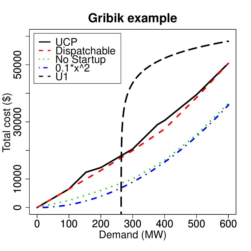
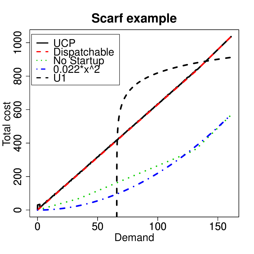
Figure 6: Cost and utility functions

The four different cost functions with the two examples are illustrated in Fig. 6. ‘UCP’ means the optimal value function $v(y)$ of the UCP (8), i.e., the actual cost function for the supplier. ‘Dispatchable’ means the optimal value function of the continuous relaxation model of (8); i.e., the model replaces the 0-1 integer constraints $z_{j}\in\{0,1\}$ in (8) by $0\leq z_{j}\leq 1$ for all $j$. The dispatchable pricing model in [5] uses a subgradient of ‘Dispatchable’ as a price. We used this model for comparison of the uplift payments. ‘No Startup’ means the optimal value function of (8) that ignores the startup cost of the generators, i.e., (8) with $S_{j}=0$ for all $j$. We also used a quadratic cost function that approximates ‘No Startup’ and that satisfies the assumption of existing convex cost models [2, 3] (i.e., Assumption 1).

We can use a smooth and convex function approximating ‘UCP’ in the existing models. However, the use of such function is unrealistic since the explicit function form of ‘UCP’ is generally too complicated to compute as we noted in Section III. Note that our model doesn’t need to calculate ‘UCP’, although our model sets a subgradient of the convex hull of ‘UCP’ as a price.

V-B Demand function

Following [3], we used the hourly demand function,

$$D_{t}(\lambda)=\mu_{1}\nu d_{1,t}+\mu_{2}(1+\delta_{2,t})d(\lambda),$$ (14)

where $\mu_{1},\mu_{2},\nu$ are positive parameters, $d_{1,t}$ is a positive constant, and $\delta_{2,t}$ is a random variable distributed with $\mathcal{N}(0,0.01^{2})$ $(t=1,2,\dots,24)$. The first term in (14) represents the minimum necessary demand, and the second term in (14) represents the swing in demand depending on prices. We used actual hourly demand data of the Tokyo Electric Power Company from 0:00 to 23:00 August 30, 2012 [14] as $d_{1,t}$ $(t=1,2,...,24)$. $\nu$ is a scale parameter to adapt the demand to the examples’ size. We defined $d(\lambda)$ as a solution of the following utility maximization problem:

$$d(\lambda):=\mathop{\rm arg~{}max}\limits_{d\geq 0}\{u(d)-\lambda d\},$$

where $u(d)$ is a logarithmic utility function $a\log(d)$ with a positive parameter $a$. Positive parameters $a$, $\mu_{1}$, $\mu_{2}$ are adjusted so that the sum of simulated hourly demands $D_{t}(\lambda_{t}^{N})$ remained nearly equal to the sum of the scaled actual hourly demands $\nu d_{1,t}$, i.e.,

$$\sum\nolimits_{t=1}^{24}D_{t}(\lambda_{t}^{N})\approx\nu\sum\nolimits_{t=1}^{24}d_{1,t}.$$

Parameter settings for the demand function (14) are shown in the TABLE III.

TABLE III: Parameter Settings for demand function (14)

	$N$	$a$	$\nu$	$\mu_{1}$	$\mu_{2}$
Gribik	100	$3.9\times 10^{4}$	0.01	0.8	0.2
Scarf	100	455	0.0025	0.8	0.2

TABLE IV: Summary of $d_{1,t}$

	min	mean	max
$d_{1,t}$	28340.0	41086.7	50780.0

V-C Utility function

In Section II, we assumed that the consumer determines their demand $D_{t}$ to maximize their utility, i.e.,

$$D_{t}(\lambda)=\mathop{\rm arg~{}max}\limits_{D\geq 0}\{U_{t}(D)-\lambda D\},$$

where $U_{t}$ is a utility function. In the case that the demand function $D_{t}$ is given by (14), $U_{t}$ can be represented as follows:

$$U_{t}(D)=a\mu_{2}(1+\delta_{2,t})\log(D-\mu_{1}\nu d_{1})+C,$$

where $C$ is a constant. The concave lines in Fig. 6 illustrate $U_{1}(D)$ with $C=20000$ for Gribik example and $C=500$ for Scarf example. The margin between $U_{1}(D)$ and ‘UCP’ represents the social welfare (3) under the condition that the supply and demand are equal.

V-D Comparison of pricing models

V-D1 Uplift payments

First, let us compare the uplift payments of our model with the convex cost model in [2, 3]. The convex cost model uses the quadratic functions in Fig. 6 as cost functions. Its electricity price is given by a locational marginal price (LMP) (see [2, 3] for details). On the other hand, our electricity price is given by the CHP. The hourly optimal prices $\lambda^{*}_{t}~{}(t=1,2,\dots,24)$ for our model were calculated with (12), whereas optimal prices for the existing convex cost model were calculated with [3, eq.(7)].

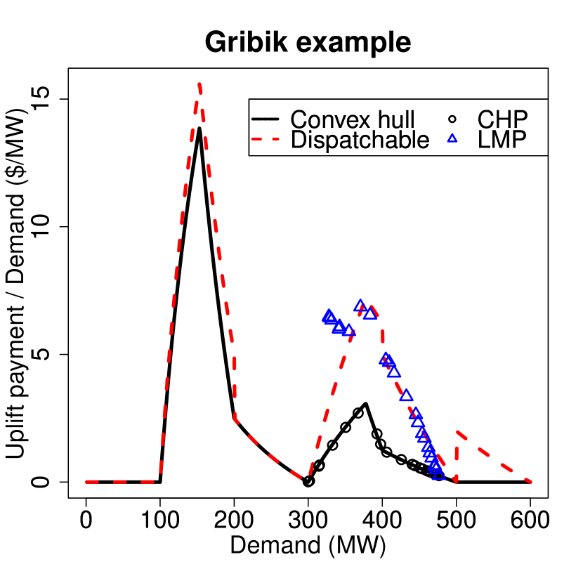
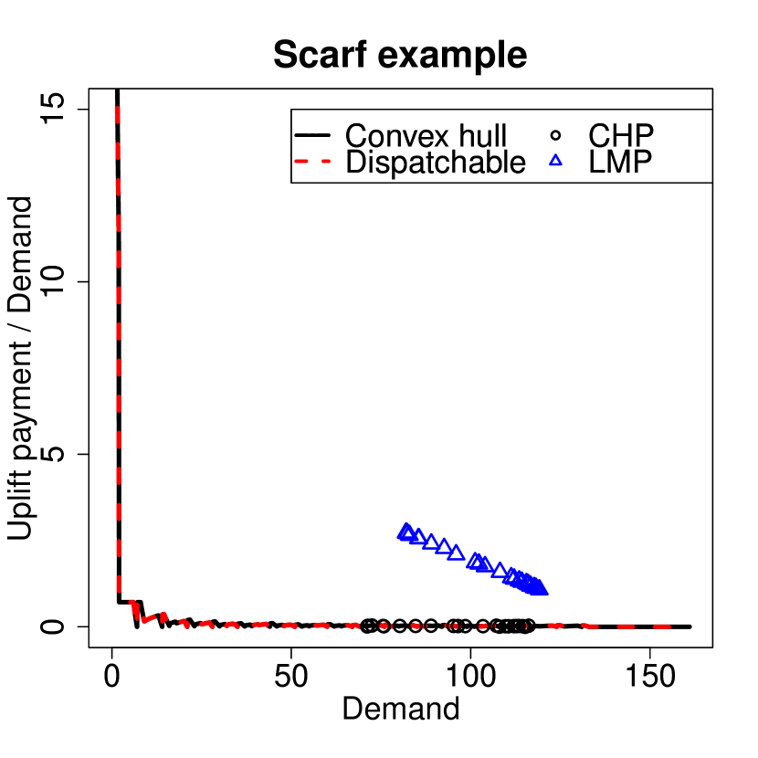
Figure 7: Comparison of uplift payments of CHPs and LMPs

Each point in Fig. 7 shows the relation between the equilibrium demand $D_{t}(\lambda_{t}^{*})$ and the uplift payments $\Pi(\lambda_{t}^{*},D_{t}(\lambda_{t}^{*}))$ for the hourly optimal prices $\lambda^{*}_{t}~{}(t=1,2,\dots,24)$. The solid (dashed) line illustrates the uplift payments with the CHP (dispatchable pricing) model in [5] at each fixed demand. Note that the solid line shows the theoretical lower bound of the uplift payments at each demand. In our model, the uplift payments accrue less than half that of the convex cost model.

V-D2 Demand, utility, and profit

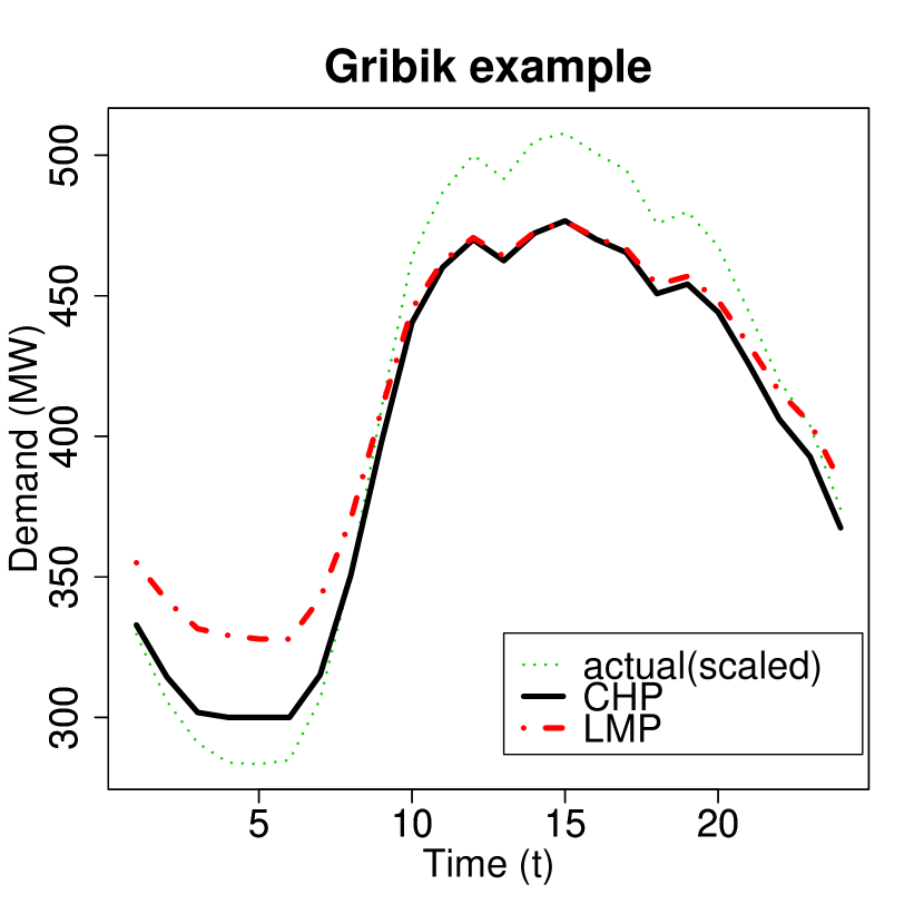
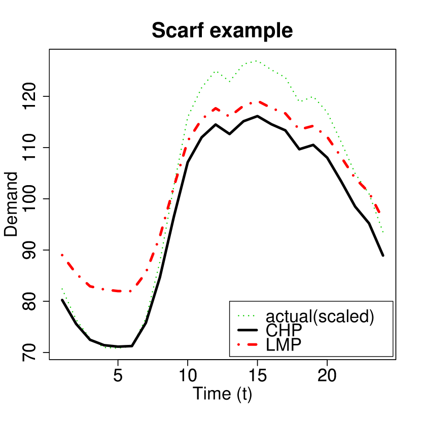
Figure 8: Hourly equilibrium demand.

Fig. 8 illustrates the hourly equilibrium demand $D_{t}(\lambda^{*}_{t})$. In each example, our model tends to lead less demand than that of the convex cost model, especially in the early morning. It is because our model tends to set higher prices than that of the existing model due to the startup costs (as shown in TABLE V); Especially at an early hour, the startup costs occupy largely in total cost.

TABLE V: Summary of simulated prices

		min	mean	max
Gribik	CHP	87.1	94.0	95.2
	LMP	65.6	82.2	95.3
Scarf	CHP	6.3	6.3	6.4
	LMP	3.6	4.5	5.2

TABLE VI: Sum of simulated results with Gribik example

	$\nu\sum d_{1,t}$	LMP	CHP
Demand	9860.8	9860.4	9570.7
Consumer’s utility	NA	354572.9	249772.4
Supplier’s profit	NA	70362.1	181574.5
Social welfare	NA	424935.0	431346.9

TABLE VII: Sum of simulated results with Scarf example

	$\nu\sum d_{1,t}$	LMP	CHP
Demand	2465.2	2465.368	2318.659
Consumer’s utility	NA	7248.106	3203.201
Supplier’s profit	NA	-4253.82	-31.5361
Social welfare	NA	2375.12	1802.465

The sum of hourly results are summarized in TABLE VI and VII. Since our model tends to set the price higher, demand and consumer’s utility would be lower and supplier’s profit would be higher. On Scarf example, the supplier’s profit takes negative value. Because it is difficult to reap profit under the price using a subgradient (or the gradient) in the case that a cost function is almost linear (even in such a case, our model achieves more preferable results for the supplier than the convex cost model). If the ISO sets higher prices than LMPs and CHPs, the supplier may make positive profit. However, such prices would increase the uplift payments.

V-D3 Social welfare

While the social welfare of our model is larger than that of the convex cost model for Gribik example, it comes out opposite results for Scarf example (see TABLEs VI and VII). Although our model minimizes the uplift payments, we cannot say that our model leads larger social welfare.

V-E Comparison of pricing algorithms

Next, let us investigate the performance of pricing algorithms. The algorithm based on the steepest descent method [3] was used for the convex cost model. We choose the step sizes, which are used in Algorithm 1 in [3] and Algorithm 2 in this paper, as $\gamma^{k}=1/10k$ for Gribik example and as $\gamma^{k}=1/100k$ for Scarf example $(k=1,2,\dots,N)$. The initial price was $\lambda^{0}_{t}=100$ for Gribik example and $\lambda^{0}_{t}=10$ for Scarf example $(t=1,2,\dots,24)$.

V-E1 Change of uplift payments with respect to iterations.

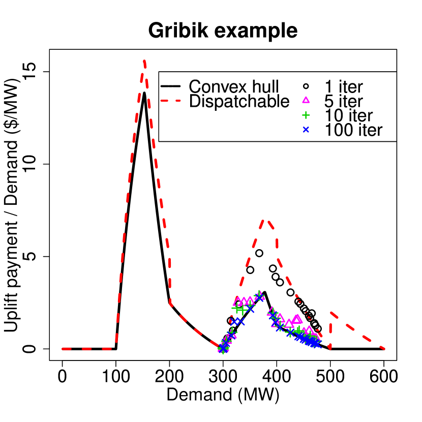
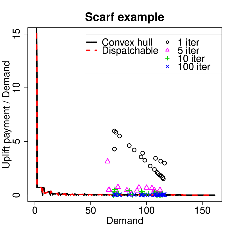
Figure 9: Uplift payments at each iteration.

Fig. 9 shows the uplift payments on the price after the $k$-th iteration $\lambda^{k}_{t}~{}(t=1,2,\dots,24,~{}k=1,5,10,100)$ of our algorithm (i.e., Algorithm 2). We can see that the prices of our algorithm achieve lower uplift payments than those of the convex cost model (i.e., ‘LMP’ in Fig. 7) in a few iteration. Furthermore, after about $10$ iterations, the uplift payments reach sufficiently close to the solid line. This implies that the prices $\lambda_{t}^{k}$ are almost the same as CHPs. Under the pricing scheme that we assumed, the market participants have to show prices or levels of consumption and production to each other at each iteration. Therefore, it is unrealistic to iterate many times. Our model shows smaller uplift payments than the convex cost model within a realistic number of iterations.

V-E2 Change of the uplift payments with respect to computational time

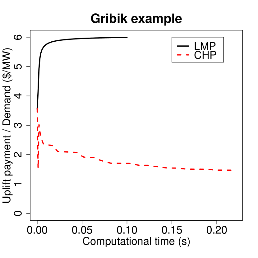
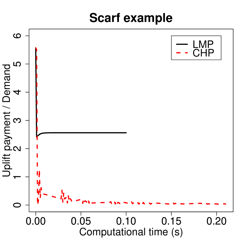
Figure 10: Change of the uplift payments with respect to computational time for 100 iterations.

While we only show the results at 1:00 (i.e., $t=2$) in Fig. 10 for lack of space, remaining time has similar numerical results. On Gribik example, the convex cost model increases the uplift payments with computational time, since the uplift payments for the initial price $\lambda^{0}_{t}$ are smaller than ones for the LMPs. By contrast, our model decreases the uplift payments with computational time. On Scarf example, the both algorithms decrease the uplift payments. The algorithm for the convex cost model (i.e., Algorithm 1 in [3]) reduces the uplift payments faster than one for our model (i.e., Algorithm 2 in this paper) at first, since it takes less computational time for an iteration. However, we can see that the algorithm for our model leads less uplift payments than one for the convex cost model a short time later.

VI Conclusion

This paper provided a new dynamic pricing model based on the CHP approach which has not been used in the context of dynamic pricing. We first considered a nonconvex cost function within the settings of the UCP, and added it to a social welfare maximization problem. We proved that a solution of its dual problem (i.e., Lagrange multiplier) gives the CHP. This implies that our model minimizes the uplift payment for an equilibrium demand. Since our model itself is formulated as a mixed integer programming problem, and moreover, the objective function of our model would be nonsmooth, it is difficult to solve our model exactly. Therefore, we provided an iterative approximation algorithm based on the subgradient method. Numerical experiment showed our pricing model led to smaller uplift payment compared with existing LMP models with convex cost functions. In addition, our pricing algorithm reduced the uplift payments in a few iterations and a little computational time.

In our numerical experiment, we used examples where generators have piece-wise linear cost functions. Thus we could use a mixed integer programming solver. We are planning to investigate ways to deal general nonlinear variable cost functions. We are also planning to extend our model to a multi-agent and multi-period one with network constraints as in [4].

Naoki Ito received his B.E. degree in Administration Engineering from Keio University, Yokohama, Japan, in 2013. He is currently working toward the M.E. degree at Keio University, Yokohama, Japan. His research interests include optimization methods for nonconvex optimization problems.

Akiko Takeda received the B.E. and M.E. degrees in Administration Engineering from Keio University, Yokohama, Japan, in 1996 and 1998, respectively, and the Dr.Sc. degree in Information Science from Tokyo Institute of Technology, Tokyo, Japan, in 2001. She is currently an Associate Professor at the Department of Mathematical Informatics at the University of Tokyo, Japan. Her research interests include solution methods for decision making problems under uncertainty and nonconvex optimization problems, which appear in financial engineering, machine learning, energy systems, etc.

Toru Namerikawa received the B.E., M.E and Ph. D of Engineering degrees in Electrical and Computer Engineering from Kanazawa University, Japan, in 1991, 1993 and 1997, respectively. He is currently an Associate Professor at Department of System Design Engineering, Keio University, Yokohama, Japan. He held visiting positions at Swiss Federal Institute of Technology in Zurich in 1998, University of California, Santa Barbara in 2001, University of Stuttgart in 2008 and Lund University in 2010. His main research interests are robust control, distributed and cooperative control and their application to power network systems.

References

- [1] N. Ito, A. Takeda, and T. Namerikawa, “Convex hull pricing for demand response in electricity markets,” in 4th IEEE Conference on Smart Grid Communications (SmartGridComm). IEEE, Oct. 2013, to appear.
- [2] M. Roozbehani, M. A. Dahleh, and S. K. Mitter, “Volatility of power grids under real-time pricing,” IEEE Transactions on Power Systems, vol. 27, no. 4, pp. 1926–1940, Nov. 2012.
- [3] Y. Miyano and T. Namerikawa, “Load leveling control by real-time dynamical pricing based on steepest descent method,” in SICE Annual Conference, Akita University, Akita, Japan, 2012, pp. 131–136.
- [4] W. Hogan and B. Ring, “On minimum-uplift pricing for electricity markets,” Harvard University, Tech. Rep., 2003. [Online]. Available: http://www.hks.harvard.edu/fs/whogan/minuplift_031903.pdf
- [5] P. R. Gribik, W. W. Hogan, and S. L. Pope, “Market-clearing electricity prices and energy uplift,” Tech. Rep., 2007. [Online]. Available: http://www.hks.harvard.edu/fs/whogan/Gribik_Hogan_Pope_Price_Uplift_123107.pdf
- [6] M. Bjørndal and K. Jörnsten, “Equilibrium prices supported by dual price functions in markets with non-convexities,” European Journal of Operational Research, vol. 190, no. 3, pp. 768–789, Nov. 2008.
- [7] B. Zhang, P. B. Luh, and E. Litvinov, “On reducing uplift payment in electricity markets,” in Power Systems Conference and Exposition, 2009. PSCE ’09. IEEE/PES, Mar. 2009.
- [8] R. P. O’Neill, P. M. Sotkiewicz, B. F. Hobbs, M. H. Rothkopf, and W. R. Stewart, “Efficient market-clearing prices in markets with nonconvexities,” European Journal of Operational Research, vol. 164, no. 1, pp. 269–285, Jul. 2005.
- [9] G. Wang, U. V. Shanbhag, T. Zheng, E. Litvinov, and S. Meyn, “An extreme-point subdifferential method for convex hull pricing in energy and reserve markets–Part I: Algorithm structure,” IEEE Transactions on Power Systems, vol. PP, no. 99, 2013, early access articles, DOI: 10.1109/TPWRS.2012.2229302.
- [10] C. Wang, P. B. Luh, G. Paul, L. Zhang, and T. Peng, “The subgradient-simplex based cutting plane method for convex hull pricing,” in Power and Energy Society General Meeting, 2010 IEEE, Jul. 2010.
- [11] M. Roozbehani, M. Dahleh, and S. Mitter, “On the stability of wholesale electricity markets under real-time pricing,” in 49th IEEE Conference on Decision and Control (CDC). IEEE, Dec. 2010, pp. 1911–1918.
- [12] D. P. Bertsekas, A. Nedic, and A. E. Ozdaglar, Convex Analysis and Optimization, ser. Optimization and Computation Series. Athena Scientific, 2003.
- [13] H. E. Scarf, “The allocation of resources in the presence of indivisibilities,” Journal of Economic Perspectives, vol. 8, no. 4, pp. 111–128, Nov. 1994. [Online]. Available: http://pubs.aeaweb.org/doi/abs/10.1257/jep.8.4.111
- [14] Tokyo Electric Power Company (TEPCO), “TEPCO electricity forecast,” http://www.tepco.co.jp/en/forecast/html/index-e.html, accessed: 2013-04-29.