Neel temperature

Phase diagram of spin-$\frac{1}{2}$ quantum Heisenberg $J_{1}-J_{2}$ antiferromagnet on the body-centered-cubic lattice in random phase approximation

Abstract

Magnetic properties of spin $\frac{1}{2}$ $J_{1}-J_{2}$ Heisenberg antiferromagnet on body centered cubic lattice are investigated. By using two-time temperature Green’s functions, sublattice magnetization and critical temperature depending on the frustration ratio $p=J_{2}/J_{1}$ are obtained in both stripe and Néel phase. The analysis of ground state sublattice magnetization and phase diagram indicates the critical end point at $J_{2}/J_{1}=0.714$, in agreement with previous studies.

1 Introduction

We are witnessing the increased interest in the study of quantum phase transitions [1, 2] in magnetic systems [3], which can be triggered by varying some of the system’s parameters. These include exchange integrals, external magnetic field, or the doping concentration in the case of high- Tc superconductors.

The motivation for studying the quantum phase transitions comes in part from closely related problem of strongly correlated systems at low temperatures. They display transition between ground state ($T=0$ K) phases as a combination of the quantum fluctuations and the competition between interactions, i.e. frustration [4]. Nowdays, a frustrated spin systems are among the most interesting and challenging topics in theoretical magnetism, including even frustrated 2D Ising model [5]. Competition between exchange interactions in magnetic materials can lead to a variety of the magnetic ordering states, and even to induce a phase transitions between them. Consequently, the frustrated quantum Heisenberg magnets with competing nearest - neighbour (NN) and next - nearest - neighbour (NNN) antriferromagnetic (AF) exchange interactions ($J_{1}$ and $J_{2}$, respectively) have become extremely active field of research.

The early works focused on the square lattice Heisenberg model, and it was investigated in detail by different methods [6, 7, 8, 9, 10, 11, 12, 13, 14, 15, 16, 17, 18]. With vanishing NNN interaction ($J_{2}=0$), the ground is state known to be antiferromagnetic (AF) for $S\geq 1$ [19]. A nonzero NNN interaction leads to the frustration and the ”crash” of simple AF ordering. For large enough $J_{2}$, the ”stripe phase” emerges [18], with possible spin-liquid phase at $J_{2}/J_{1}\approx 0.5$. (See [20] and references therein). We shall be interested in 3D version of the problem, with localized spins arranged on a body-centered-cubic (bcc) lattice. The mean field calculation [21] indicates existence of two phases, represented with different spin orderings on the Figure 1. Néel state (AF1) can be described by a standard two-sublattice system, while the proper treatment of the stripe phase (AF2) can be accomplished by the introduction of four sublattices.

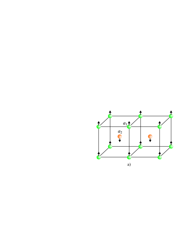
Figure 1: (Color online) a) Néel ordering denoted as AF1 phase in further text. b) stripe ordering denoted as AF2 phase in further text (after [21]).

The transition between two phases is governed by the frustration ratio $p=J_{2}/J_{1}$ and the mean-field calculation gives $p_{\mathrm{MF}}=2/3$ for its critical value [22]. Numerous sophisticated methods were subsequently used to obtain more reliable value of the critical frustration ratio. Schmidt et al. [23] carried out exact diagonalization of finite 3D lattices with periodic boundary conditions. Ground state energy was found to have a discontinuity at $p=0.693$ indicating a first order quantum transition between two phases. This was confirmed by calculation of magnetization and extrapolation to infinite lattice. J. Oitmaa and W. Zhang [22] performed high-order linked-cluster expansion at $T=0K$ and obtained that two branches of ground state energy for AF1 and AF2 phases cross at $J_{2}/J_{1}=0.705\pm 0.005$. Majumdar and Datta [24] presented a non-linear spin wave theory (up to quartic terms in Bose-operators) giving quite similar results. Majumdar [25] also extended this problem to the antiferromanget on stacked square lattices with different exchange in vertical direction.

The aim of this paper is to present, up to the our knowledge, the first application of spin operator Green’s functions on spin-$\frac{1}{2}$ bcc lattice $J_{1}-J_{2}$ Heisenberg antiferromagnet. It will be shown that spin operator temperature Green function (TGF) method, in combination with random phase approximation (RPA), yields reliable results both at $T=0$K and at critical temperature. The paper is organized as follows. The RPA magnon spectrum in both AF1 and AF2 phase is determined in the Section 2. The calculation of ground state sublattice magnetization is presented in Section 3, while Section 4 contains discussion on the Néel temperature and phase diagram. Finally, Section 5 concludes the paper.

2 Magnon Spectrum

2.1 AF1 (Néel) phase

We start with the spin-$\frac{1}{2}$ Hamiltonian of the system with two sublattices $a_{1}$ and $a_{2}$ (See Figure 1 a)):

$$\hat{H}_{\mathrm{AF1}} = J_{1}\sum_{\bm{n},\bm{\lambda}}\hat{{\color[rgb]{0.3,0.7,0.345}\bm{S}}}_{\bm{n}}^{(a_{1})}\cdot\hat{{\color[rgb]{1,0.49,0}\bm{S}}}_{\bm{n}+\bm{\lambda}}^{(a_{2})}+\frac{J_{2}}{2}\sum_{\bm{n},\bm{\delta}}\hat{{\color[rgb]{0.3,0.7,0.345}\bm{S}}}_{\bm{n}}^{(a_{1})}\cdot\hat{{\color[rgb]{0.3,0.7,0.345}\bm{S}}}_{\bm{n}+\bm{\delta}}^{(a_{1})}$$ (1)

$$+ \frac{J_{2}}{2}\sum_{\bm{n},\bm{\delta}}\hat{{\color[rgb]{1,0.49,0}\bm{S}}}_{\bm{n}}^{(a_{2})}\cdot\hat{{\color[rgb]{1,0.49,0}\bm{S}}}_{\bm{n}+\bm{\delta}}^{(a_{2})}.$$

Here $\bm{n}$ denotes the site in the given sublattice, each having $N_{\mathrm{N}}=N/2$ sites and both exchange parameters $(J_{1},J_{2})$ are assumed to be positive. $\bm{\lambda}$ connects first neighbours from sublattices $a_{1}$ and $a_{2}$, while $\bm{\delta}$ relates corresponding second neighbours. It is seen from Figure 1 that every site has $z_{1}=8$ nearest neighbours and that the number of second neighbours is $z_{2}=6$. To simplify calculations we rotate operators from $a_{2}$ sublattice about $S^{x}$ axis by $\pi$ as in [26, 27].

Writing down four equations of motion for Green’s functions $G_{1}\equiv\langle\langle{\color[rgb]{0.3,0.7,0.345}S}^{+(a_{1})}|{\color[rgb]{0.3,0.7,0.345}S}^{-(a_{1})}\rangle\rangle,\;\;G_{2}\equiv\langle\langle{\color[rgb]{1,0.49,0}S}^{-(a_{2})}|{\color[rgb]{0.3,0.7,0.345}S}^{-(a_{1})}\rangle\rangle$, and employing RPA decoupling procedure [26, 28, 29, 30, 31, 32], we find one-magnon energies

$$E(\bm{k})=z_{1}J_{1}\langle S^{z}\rangle\sqrt{\left[1-p\;\frac{z_{2}}{z_{1}}(1-\gamma_{2}(\bm{k}))\right]^{2}-\gamma_{1}(\bm{k})^{2}},$$ (2)

where

$$\gamma_{1}(\bm{k})=\frac{1}{z_{1}}\sum_{\bm{\lambda}}\mbox{e}^{i\bm{k}\cdot\bm{\lambda}},\;\;\;\gamma_{2}(\bm{k})=\frac{1}{z_{2}}\sum_{\bm{\delta}}\mbox{e}^{i\bm{k}\cdot\bm{\delta}}.$$ (3)

In the absence of external magnetic field, the magnon spectrum is doubly degenerate as there are two types of magnons with energies given in (2). Figure 2 shows the $k_{z}=0$ intersection of reduced magnon energies $\omega(\bm{k})=E(\bm{k})/(J_{1}z_{1}\langle S^{z}\rangle)$. It can be clearly seen that the spectrum contains the Goldstone mode. An important feature of RPA decoupling scheme is magnon energy renormalization. Compared to LSW results [23], RPA magnon energies are renormalized by a factor of $\langle S^{z}\rangle/S$, which includes the effects of magnon-magnon interactions in RPA. As a consequence, the plot of sublattice magnetization from Figure 4 suggests that elementary excitations are not well defined starting at $p\sim 0.7$.

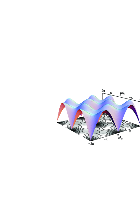
Figure 2: (Color online) Reduced magnon energies $\omega(\bm{k})=E(\bm{k})/(J_{1}z_{1}\langle S^{z}\rangle)$ for $k_{z}=0$, $p=0.5$ in AF1 phase.

2.2 AF2 (stripe) phase

Next we turn to the AF2 phase. The spin Hamiltonian is

$$\hat{H}_{\mathrm{AF2}} = J_{1}\sum_{\bm{n},\bm{\lambda}_{13}}\hat{{\color[rgb]{0.55,0.14,1}\bm{S}}}_{\bm{n}}^{(a_{1})}\cdot\hat{{\color[rgb]{1,0,0}\bm{S}}}_{\bm{n}+\bm{\lambda}_{13}}^{(a_{3})}+J_{1}\sum_{\bm{n},\bm{\lambda}_{14}}\hat{{\color[rgb]{0.55,0.14,1}\bm{S}}}_{\bm{n}}^{(a_{1})}\cdot\hat{{\color[rgb]{0.3,0.7,0.345}\bm{S}}}_{\bm{n}+\bm{\lambda}_{14}}^{(a_{4})}$$ (4)

$$+ J_{1}\sum_{\bm{n},\bm{\lambda}_{23}}\hat{{\color[rgb]{1,0.49,0}\bm{S}}}_{\bm{n}}^{(a_{2})}\cdot\hat{{\color[rgb]{1,0,0}\bm{S}}}_{\bm{n}+\bm{\lambda}_{23}}^{(a_{3})}+J_{1}\sum_{\bm{n},\bm{\lambda}_{24}}\hat{{\color[rgb]{1,0.49,0}\bm{S}}}_{\bm{n}}^{(a_{2})}\cdot\hat{{\color[rgb]{0.3,0.7,0.345}\bm{S}}}_{\bm{n}+\bm{\lambda}_{24}}^{(a_{4})}$$

$$+ J_{2}\sum_{\bm{n},\bm{\delta}}\hat{{\color[rgb]{0.55,0.14,1}\bm{S}}}_{\bm{n}}^{(a_{1})}\cdot\hat{{\color[rgb]{1,0.49,0}\bm{S}}}_{\bm{n}+\bm{\delta}}^{(a_{2})}\;\;\;+J_{2}\sum_{\bm{n},\bm{\delta}}\hat{{\color[rgb]{1,0,0}\bm{S}}}_{\bm{n}}^{(a_{3})}\cdot\hat{{\color[rgb]{0.3,0.7,0.345}\bm{S}}}_{\bm{n}+\bm{\delta}}^{(a_{4})}.$$

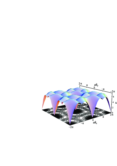
Figure 3: (Color online) Reduced magnon energies $\omega_{1}(\bm{k})=E_{1}(\bm{k})/(J_{2}z_{2}\langle S^{z}\rangle)$ for $k_{z}=0$, $p=1$ in AF2 phase.

Each of the sublattices in AF2 phase consists of $N_{\mathrm{S}}=N/4$ sites so that $\{\bm{\lambda}_{ij}\}$ connects first neighbours from sublattices $a_{i}$ and $a_{j}$ and $\{\bm{\delta}\}$ are the same vectors as in AF1 phase. Also, it is seen from Figure 1 that all lattice sites in AF2 phase have equal number ($z_{1}=4$) of nearest neighbours in two different sublattices.

Using equations of motion for the Green’s functions $\mathcal{G}_{1}\equiv\langle\langle{\color[rgb]{0.55,0.14,1}S}^{{\color[rgb]{0.55,0.14,1}+}(a_{1})}|{\color[rgb]{0.55,0.14,1}S}^{{\color[rgb]{0.55,0.14,1}-}(a_{1})}\rangle\rangle,\;\;\mathcal{G}_{2}\equiv\langle\langle{\color[rgb]{1,0.49,0}S}^{{\color[rgb]{1,0.49,0}-}(a_{2})}|{\color[rgb]{0.55,0.14,1}S}^{{\color[rgb]{0.55,0.14,1}-}(a_{1})}\rangle\rangle,\;\;\mathcal{G}_{3}\equiv\langle\langle{\color[rgb]{1,0,0}S}^{{\color[rgb]{1,0,0}+}(a_{3})}|{\color[rgb]{0.55,0.14,1}S}^{{\color[rgb]{0.55,0.14,1}-}(a_{1})}\rangle\rangle$, $\mathcal{G}_{4}\equiv\langle\langle{\color[rgb]{0.3,0.7,0.345}S}^{{\color[rgb]{0.3,0.7,0.345}-}(a_{4})}|{\color[rgb]{0.55,0.14,1}S}^{{\color[rgb]{0.55,0.14,1}-}(a_{1})}\rangle\rangle$, together with RPA linearization, we find renormalized one-magnon energies

$$E_{1,2}(\bm{k})=z_{2}J_{2}\langle S^{z}\rangle\sqrt{\left[1-\gamma_{2}(\bm{k})^{2}\right]\pm\left(\frac{z_{1}}{z_{2}p}\right)^{2}K(\bm{k})},$$ (5)

where $K(\bm{k})$ is the positive square root of

$$\left[\Gamma_{1}(\bm{k})^{2}-\Gamma_{1}^{*}(\bm{k})^{2}\right]^{2}+4\left(\frac{pz_{2}}{z_{1}}\right)^{2}|\Gamma_{1}^{*}(\bm{k})-\Gamma_{1}(\bm{k})\gamma_{2}(\bm{k})|^{2}.$$ (6)

Also

$$\Gamma_{1}(\bm{k}) = \frac{1}{z_{1}}\sum_{\bm{\lambda}_{14}}\mbox{e}^{i\bm{k}\cdot\bm{\lambda}_{14}}=\frac{1}{z_{1}}\sum_{\bm{\lambda}_{23}}\mbox{e}^{i\bm{k}\cdot\bm{\lambda}_{23}}$$

$$\Gamma_{1}^{*}(\bm{k}) = \frac{1}{z_{1}}\sum_{\bm{\lambda}_{13}}\mbox{e}^{i\bm{k}\cdot\bm{\lambda}_{13}}=\frac{1}{z_{1}}\sum_{\bm{\lambda}_{24}}\mbox{e}^{i\bm{k}\cdot\bm{\lambda}_{24}}$$ (7)

while $\gamma_{2}(\bm{k})$ is defined in (3). Each of magnon energies from (5) is doubly degenerate so that the total number of magnon flavours in the stripe phase is four. All four magnon branches survive in the limit $J_{1}\rightarrow 0$ (i.e. $p\rightarrow\infty$) when system described by (4) reduces to the two decoupled antiferromagnets with Néel order on simple cubic lattices. The magnon spectrum (5) then simplifies to $E(\bm{k})=J_{2}z_{2}\langle S^{z}\rangle\sqrt{1-\gamma_{2}(\bm{k})^{2}}$ so that all four flavours have the same dispersion. As an illustration of the magnon spectrum in the stripe phase, we plot $\omega(\bm{k})=E_{1}(\bm{k})/(J_{1}z_{2}\langle S^{z}\rangle)$ for $k_{z}=0$ and $p=1$ on Figure 3. As in the AF1 phase, magnon-magnon interactions induced by RPA renormalize the magnon energies. It is seen from Figure 4 that instability of AF2 phase starts at $p\lesssim 0.7$.

Now that the renormalized magnon spectrum is determined, including effects of frustration, we can examine its influence on thermodynamics of spin $\frac{1}{2}$ bcc lattice $J_{1}-J_{2}$ Heisenberg antiferromagnet. We have to bear in mind, however, that for correct calculation of thermodynamic properties in RPA, one must take the full set of the poles of Green’s functions from single system of equations [33]. These are $\{E(\bm{k}),-E(\bm{k})\}$ in the Néel phase and $\{E_{1}(\bm{k}),-E_{1}(\bm{k}),E_{2}(\bm{k}),-E_{2}(\bm{k})\}$ in the stripe phase. We stress once again that only positive poles of the Green’s functions represent energies of physical magnons.

3 Sublattice magnetization

Standard spectral theorem enable us to find the ground state sublattice magnetization in AF1 phase

$$\langle S^{z}\rangle_{0} = \frac{1}{2}\left(\frac{1}{N_{\mathrm{N}}}\sum_{\bm{k}}\frac{\varepsilon_{1}(\bm{k})}{E(\bm{k})}\right)^{-1},$$ (8)

where

$$\varepsilon_{1}(\bm{k}) = \langle S^{z}\rangle\left[z_{1}J_{1}-z_{2}J_{2}+z_{2}J_{2}\gamma_{2}(\bm{k})\right],$$ (9)

and in AF2 phase

$$\langle S^{z}\rangle^{-1}_{0}=\frac{p}{N_{\mathrm{S}}}\sum_{\bm{k}}\frac{1}{K(\bm{k})K_{1}(\bm{k})K_{2}(\bm{k})}$$ (11)

$$\times \left\{\left[6[K(\bm{k})+2|\Gamma_{1}(\bm{k})|^{2}]-[\Gamma_{1}(\bm{k})^{2}+\Gamma_{1}^{*}(\bm{k})^{2}]\gamma_{2}(\bm{k})\right]K_{2}(\bm{k})\right.$$

$$+ \left.\left[6[K(\bm{k})-2|\Gamma_{1}(\bm{k})|^{2}]+[\Gamma_{1}(\bm{k})^{2}+\Gamma_{1}^{*}(\bm{k})^{2}]\gamma_{2}(\bm{k})\right]K_{1}(\bm{k})\right\},$$

$$K_{i}(\bm{k})=\frac{E_{i}(\bm{k})}{z_{2}J_{2}\langle S^{z}\rangle},\hskip 28.45274pti=1,2.$$

the plot of which is given at at Figure 4. As noted earlier in the text, the behaviour of antiferromagnetic order parameter suggest the phase transition between AF1 and AF2 phase at $p\approx 0.7$.

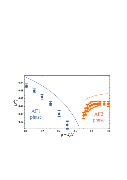
Figure 4: (Color online) Sublattice magnetization at $T=0$K in AF1 and AF2 phase (Equations (8) and (11)). The curves represent RPA result, while dots are linked-cluster values expansions taken from [22]

We also observe that RPA results for sublattice magnetization are in agreement with high-order linked-cluster expansions at $T=0$ of Oitmaa and Zheng [22], since relative difference between these methods is $\approx 2\%$. Similarly, our values for the order parameter in AF1 and AF2 phase are quite close to the ones obtained from self-consistent non-linear spin wave theory [24]. For example, it can be shown [34] that for $J_{2}=0$, equation (8) gives $\langle S^{z}\rangle_{0}=\frac{1}{2}\left[{}_{4}F_{3}\left(\frac{1}{2},\frac{1}{2},\frac{1}{2},\frac{1}{2};1,1,1;1\right)\right]^{-1}\approx 0.446973$, while non-linear self-consistent spin-wave theory yields $\langle S^{z}\rangle_{0}=1-(1/2)\;_{4}F_{3}\left(\frac{1}{2},\frac{1}{2},\frac{1}{2},\frac{1}{2};1,1,1;1\right)\approx 0.440682$. Here, ${}_{4}F_{3}\left(\frac{1}{2},\frac{1}{2},\frac{1}{2},\frac{1}{2};1,1,1;1\right)$ denotes the hypergeometric function.

4 Néel Temperature and Phase Diagram

Following [26, 28, 29], we find the critical temperature in the Néel phase

$$T_{\mathrm{N}}^{\mathrm{AF1}}(p) = \frac{2J_{1}}{I(p)}$$ (12)

$$I(p) = \frac{1}{N_{\mathrm{N}}}\sum_{\bm{k}}\frac{1-p[z_{2}/z_{1}][1-\gamma_{2}(\bm{k})]}{\{1-p[z_{2}/z_{1}][1-\gamma_{2}(\bm{k})]\}^{2}-\gamma_{1}(\bm{k})^{2}}.$$

The general RPA expression for critical temperature remains the same, but in the stripe phase integral $I(p)$ gets replaced by $\mathcal{I}(p)$, defined by

$$\frac{p}{N_{\mathrm{S}}}\sum_{\bm{k}}\frac{6[K(\bm{k})+2|\Gamma_{1}(\bm{k})|^{2}]-[\Gamma_{1}(\bm{k})^{2}+\Gamma_{1}^{*}(\bm{k})^{2}]\gamma_{2}(\bm{k})}{K(\bm{k})K_{1}(\bm{k})^{2}}$$

$$+ \frac{p}{N_{\mathrm{S}}}\sum_{\bm{k}}\frac{6[K(\bm{k})-2|\Gamma_{1}(\bm{k})|^{2}]+[\Gamma_{1}(\bm{k})^{2}+\Gamma_{1}^{*}(\bm{k})^{2}]\gamma_{2}(\bm{k})}{K(\bm{k})K_{2}(\bm{k})^{2}}.$$

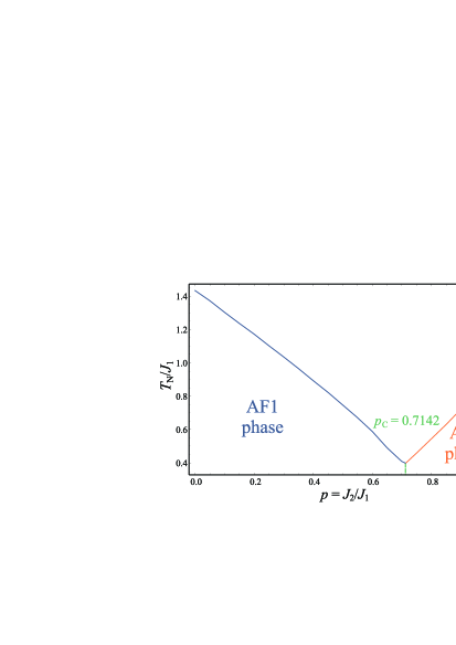
Figure 5: (Color online) The phase diagram of spin-$\frac{1}{2}$ bcc lattice $J_{1}-J_{2}$ Heisenberg model

Figure 5 shows our results for reduced critical temperature ($T_{N}/J_{1}$) in terms of frustration ratio $J_{2}/J_{1}$. The indication of first-order transition at $T=0$K and $p_{c}\approx 0.7$ from Figure 4 is further justified by inspection of the phase diagram (see Figure 5), giving $p_{c}=0.714$. The blue and orange lines represent AF1-paramagnetic and AF2-paramagnetic transition, respectively, while the vertical (green) line shows AF1-AF2 transition line connecting the critical end point and the phase transition at $T=0$K. RPA phase diagram agrees rather well with the one obtain by high-temperature series expansion [22]. The relative difference between high-temperature series expansion and RPA values for the critical frustration ratio illustrates this nicely, since it is $\approx 1.27\%$.

5 Conclusion

In summary, we investigated the magnetic properties of spin $\frac{1}{2}$ bcc lattice $J_{1}-J_{2}$ Heisenberg antiferromagnet . Using the method of TGF’s, we obtained the phase diagram as a function of the frustration ratio $p=J_{2}/J_{1}$. Our calculations indicate instability of the long range order in AF1 and AF2 phase for $p_{c}=0.714$. This is in good agreement with previous results found by high-temperature series expansion [22]. Also, the RPA predictions for sublattice magnetization are very close to high-order linked-cluster expansions at $T=0$ [22] and non-linear self-consistent spin wave theory [24]. The main advantage of RPA TGF method over previously quoted ones is its successful applicability on both low and high temperatures.

Acknowledgment

This work was supported by the Serbian Ministry of Education and Science: Grant No 171009.

References

- [1] S. Sachdev, Quantum Phase Transitions, Canbridge University Press, 2011.
- [2] X. G. Wen, Quantum Field Theory of Many Body Systems, Oxford University Press, 2007.
- [3] T.H. Diep, Frustrated Spin Systems, 1st ed. World Scientific, Singapore, 2004.
- [4] Introduction to Frustrated Magnetism, edited by C. Lacroix, P. Mendels and F. Mila, Springer, New York, 2011.
- [5] S. Jin, A. Sen, A.W. Sandvik, Phys. Rev. Lett. 108 (2012) 045702.
- [6] H.J. Schulz and T.A.L. Ziman, Europhys. Lett. 18 (1992) 355.
- [7] H.J. Schulz, T.A.L. Ziman, and D. Poilblanc, J. Phys. I 6 (1996) 675.
- [8] J. Richter, Phys. Rev. B 47, (1993) 5794.
- [9] K. Retzlaff, J. Richter, and N.B. Ivanov, Z. Phys. B: Condens. Matter 93 (1993) 21.
- [10] J. Richter, N.B. Ivanov, and K. Retzlaff, Europhys. Lett. 25 (1994) 545.
- [11] R.F. Bishop, D.J.J. Farnell, and J.B. Parkinson, Phys. Rev. B 58 (1998) 6394.
- [12] R.R.P. Singh, Zheng Weihong, C.J. Hamer, and J. Oitmaa, Phys. Rev. B 60 (1999) 7278.
- [13] V.N. Kotov and O.P. Sushkov, Phys. Rev. B 61 (2000) 11820.
- [14] L. Capriotti and S. Sorella, Phys. Rev. Lett. 84 (2000) 3173.
- [15] O.P. Sushkov, J. Oitmaa, and Zheng Weihong, Phys. Rev. B 63 (2001) 104420.
- [16] L. Capriotti, F. Becca, A. Parola, and S. Sorella, Phys. Rev. Lett. 87 (2001) 097201.
- [17] Wang H.-Y., Phys. Rev. B 86 (2013) 144411.
- [18] N. Read, S. Sachdev, Phys. Rev. Lett. 66 (1991) 1773.
- [19] E. Manousakis, Rev. Mod. Phys. 63 (1991) 1.
- [20] E. Fradkin, Field Theories of Condensed Matter Physics, Canbridge University Press, 2013.
- [21] J.S. Smart, Effective Field Theories of Magnetism, Saunders, Philadelphia, 1966.
- [22] J. Oitmaa and W. Zhang, Phys. Rev. B 69 (2004) 064416.
- [23] R. Schmidt, J. Schulenburg, J. Richter, and D.D. Betts, Phys.Rev. B 66 (2002) 224406.
- [24] K. Majumdar and T.Datta, J. Phys. Cond. Matt. 21 (2009) 406004.
- [25] K. Majumdar, J. Phys. Cond. Matt. 23 (2011) 116004.
- [26] S. Radošević, M. Pantić, M. Rutonjski, D. Kapor, M. Škrinjar, Eur. Phys. J. B 68 (2009) 511.
- [27] S. Radošević, M. Rutonjski, , M. Pantić, M. Pavkov-Hrvojević, D. Kapor, M. Škrinjar, Solid State Commun., 151 (2011) 1753.
- [28] P. Fröbrich, P.J. Kuntz, Many-body Green’s function theory of Heisenberg films, Physics Reports, 432 (2006) 223.
- [29] W. Nolting, A. Ramakanth, Quantum Theory of Magnetism, Springer-Verlag, Berlin, 2009.
- [30] M. Manojlović, M.P. Hrvojević, M. Škrinjar, M. Pantić, D. Kapor, S. Stojanović, Phys. Rev. B 68 (2003) 014435.
- [31] M. Rutonjski, S. Radoševic, M. Škrinjar, M. Pavkov-Hrvojević, D. Kapor, M. Pantić, Phys. Rev. B, 76 (2007) 172506.
- [32] M. Rutonjski, S. Radošević, M. Pantić, M. Pavkov-Hrvojević, D. Kapor, M. Škrinjar, Solid State Commun., 151 (2011) 518.
- [33] M. Pantić, M. Škrinjar, D. Kapor, Physica A 387 (2008) 5786.
- [34] S. Radošević, M. Pantić, D. Kapor, M. Pavkov-Hrvojević and M. Škrinjar, J. Phys. A: Math. Theor. 43 (2010) 155206.