A direct dynamical measurement of the Milky Way’s disk surface density profile, disk scale length, and dark matter profile at
Abstract
We present and apply rigorous dynamical modeling with which we infer unprecedented constraints on the stellar and dark matter mass distribution within our Milky Way (MW), based on large sets of phase-space data on individual stars. Specifically, we model the dynamics of 16,269 G-type dwarfs from SEGUE, which sample and . We independently fit a parameterized MW potential and a three-integral, action-based distribution function (DF) to the phase-space data of 43 separate abundance-selected sub-populations (MAPs), accounting for the complex selection effects affecting the data. We robustly measure the total surface density within of the mid-plane to over . Using metal-poor MAPs with small radial scale lengths as dynamical tracers probes , while MAPs with longer radial scale lengths sample . We measure the mass-weighted Galactic disk scale length to be , in agreement with the photometrically inferred spatial distribution of stellar mass. We thereby measure dynamically the mass of the Galactic stellar disk to unprecedented accuracy: and a total local surface density of of which is contributed by stars and stellar remnants. By combining our surface density measurements with the terminal velocity curve, we find that the MW’s disk is maximal in the sense that at . We also constrain for the first time the radial profile of the dark halo at such small Galactocentric radii, finding that with at 95 % confidence. Our results show that action-based distribution-function modeling of complex stellar data sets is now a feasible approach that will be fruitful for interpreting Gaia data.
Subject headings:
Galaxy: abundances — Galaxy: disk — Galaxy: fundamental parameters — Galaxy: kinematics and dynamics — Galaxy: structure — solar neighborhood1. Introduction
The mass distribution of the Milky Way inside is uncertain in many respects. While good measurements exist of the rotation curve, these do not allow the separation of the major Galactic components: bulge, halo, and stellar and gas disks. Hence the relative contributions as well as the density profiles of these components are still very uncertain. Determining these is fundamental to our understanding of the Milky Way’s formation and evolution and to evaluating the importance of dark matter within the visible extent of galaxies. Because the Milky Way is in many ways an anchor point for empirical relations used to determine the physical properties of external galaxies, this ultimately has a large impact on the study of the low-redshift Universe (Rix & Bovy, 2013).
The structure, size, and mass of the Milky Way’s disk in particular are poorly known. Measurements of the radial scale length of the disk over the last few decades have produced values anywhere in between and (see, e.g., Sackett 1997 for an overview). While photometric measurements have improved with the advent of wide-area surveys with accurate photometry, systematic uncertainties in the distance scale significantly limit the precision and accuracy of photometrically measured scale lengths (e.g., Jurić et al., 2008), and such measurements only trace the radial luminosity profile of the tracer stars rather than the mass profile of the disk. This is especially problematic as it has recently become clear that the stellar disk contains abundance-distinct subcomponents with scale lengths ranging from to (Bovy et al., 2012d), and in particular that the thicker disk components in the Milky Way have a much shorter scale length than the thin disk (Bensby et al., 2011; Bovy et al., 2012d; Cheng et al., 2012). Thus, more than ever it is important to measure the mass-weighted radial profile, which can be achieved using the dynamics of tracer populations. There are currently no plausible dynamical measurements of the scale length of the disk. While there are global potential fits to a variety of dynamical data (e.g., McMillan, 2011), these cannot measure the scale length without strong prior assumptions as there have been no dynamical data and models that constrain the disk scale length to date; because of this, the disk’s scale length is the most important unknown in disentangling the contributions from the disk and the dark halo to the mass distribution near the disk (Dehnen & Binney, 1998).
In external galaxies, rotation curves are often decomposed into disk and halo contributions using the maximum-disk hypothesis (van Albada & Sancisi, 1986): the disk component is assumed to contribute the maximum amount possible without exceeding the rotation curve anywhere; in practice this means that such maximal disks contribute of the rotation velocity at the peak of the disk rotation curve, allowing for the contribution of a bulge and a cored halo (Sackett, 1997). Observational evidence for or against the maximum-disk hypothesis is scant: e.g., Courteau & Rix (1999) argues against spiral galaxy disks being generically maximal based on the residuals from the Tully-Fisher relation, while detailed gas kinematics shows that some disks, particularly fast rotators, are maximal (e.g., Weiner et al., 2001; Kranz et al., 2003) (see 6.3 for more discussion of this). Ultimately, this is due to the fact that directly measuring and decomposing the mass profile of external disks is close to impossible. However, because mass-to-light ratios for external spiral galaxies are calibrated using the maximum-disk hypothesis (e.g., Bell & de Jong, 2001), the fate of the maximum-disk hypothesis is intimately connected with many conclusions regarding the stellar-mass content of the low-redshift Universe (e.g., Bell et al., 2003; Li & White, 2009). Whether the Milky Way has a maximum disk is unknown (Sackett, 1997) and determining whether it does is important since it can provide a robust data point for the discussion of the maximum-disk hypothesis and because it could be used to calibrate dynamical measurements of the radial profile of external galaxies. Because the local midplane density and the local surface density are reasonably well measured (e.g., Kuijken & Gilmore, 1989b; Holmberg & Flynn, 2000), whether the Milky Way’s disk is maximal hinges on whether it has a short stellar disk mass scale length.
Because the rotation curve reflects the sum of the radial in-plane accelerations contributed by the various Galactic components, precise measurements of the radial profile and mass of only the disk also allows the radial profile of the dark-matter halo to be constrained. Measurements of the local density of dark matter have significantly improved recently (Bovy & Tremaine, 2012; Zhang et al., 2013), but there are no dynamical constraints on the radial profile of dark matter at . The large microlensing optical depth measured toward the bulge argues for a relatively shallow halo profile (Binney & Evans, 2001), although this constraint has been relaxed compared to Binney & Evans (2001) due to the downward revision of the optical depth (e.g., Popowski et al., 2005) and of the local dark matter density since 2001 (Bovy & Tremaine, 2012; Zhang et al., 2013). Measuring the radial profile of dark matter in the inner Milky Way would be invaluable for analyses of dark-matter indirect detection toward the Galactic center and for comparing the Milky Way to the predictions from cosmological simulations: A Milky-Way-like galaxy is presumed to have an inner dark-matter profile close to the Navarro-Frenk-White (NFW; Navarro et al. 1997) profile seen in simulations or steeper due to the adiabatic contraction that is expected to occur when the Milky Way’s massive disk forms within the dark matter halo.
In this paper, we constrain the mass distribution in the inner Milky Way by measuring the vertical force at as a function of radius between and . Because the vertical force and the surface density are approximately proportional near the disk (Kuijken & Gilmore, 1989a; Bovy & Tremaine, 2012), this quite directly measures the radial surface-density profile near the disk, allowing the mass-weighted scale length of the disk to be obtained without any prior assumptions derived from stellar number counts; we measure the radial profile of the mass rather than that of the luminosity.
We measure the vertical force as a function of radius using modeling based on simple, parameterized, six-dimensional (phase-space), three-action distribution-functions (DFs), developed by Binney (2010, 2012b) and McMillan & Binney (2013). In Ting et al. (2013) we showed that this approach should work well when applied to subsets of Galactic disk stars with very similar elemental abundances, so called mono-abundance populations (MAPs). In a recent series of papers, we (Bovy et al., 2012c, d) demonstrated that these constitute structurally-simple disk populations. Such populations can hence be described well by few-parameter families of distribution functions, which allows a full likelihood-based exploration of the joint posterior distribution function (PDF) of dynamical (gravitational potential) and DF parameters. In this paper, we apply this methodology for the first time to a real data set, G-type dwarfs from the SDSS/SEGUE survey (Yanny et al., 2009). Each MAP, i.e., each distinct, abundance-selected stellar subset, can act as a separate tracer population of the gravitational potential. We focus our efforts in this paper on measuring the dynamical quantity of interest that is most robustly determined for each MAP. This turns out to be the vertical force at at a single Galactocentric radius for each MAP, where the radius is determined directly from the dynamical PDF for each MAP; because the MAPs span a wide range in orbital distributions, this leads to measurements between and for 43 MAPs.
We use these new measurements in combination with constraints on the rotation curve, primarily from terminal-velocity measurements, and with measurements of the local vertical profile of the vertical force to constrain the mass distribution at and its decomposition into disk and dark halo contributions. Because our measurements are at , we strongly constrain the properties of the Milky Way’s disk, finding a relatively short mass scale length of and deriving precise measurements of the local column density of stars and of the total mass in the disk. We find that the Milky Way’s disk is maximal, providing about of the rotational support at 2.2 radial scale lengths (; the rotational support is ). As the halo contributes very little to the rotation curve and the vertical force at , we only weakly constrain the radial profile of the dark matter, but we nevertheless obtain a first constraint: at 95 % confidence for a model in which .
The outline of this paper is as follows. We describe the SEGUE G-dwarf data in 2. In 3 we explain in detail the various steps involved in the dynamical modeling of abundance-selected populations of stars using a DF model. We present the results from this modeling in 4.1 and discuss how we turn these results into a measurement of the surface density to at a single radius for each MAP. We show the resulting surface-density and vertical-force profiles in 4.2 and discuss systematics associated with this measurement in 4.3. In 5, we use these new measurements together with additional dynamical data to fit mass models of the inner Milky Way. We discuss the implications of these new measurements in 6. We recapitulate our main conclusions in 7 and look ahead to the dynamical analysis of Gaia data. Appendix A gives technical details of the calculation of the effective survey volume required in the dynamical modeling, and Appendix B presents various detailed comparisons between the spatial and kinematical distribution of the data and that of our best-fit dynamical models. We recommend that readers not interested in the technical details of the dynamical models read the introduction of 3, which briefly summarizes the main ingredients of the modeling, and then 4.2 for the measurement of the vertical-force profile, and 5 and following Sections for the implications of these new measurements for the mass distribution in the inner Milky Way. In this paper, we use BO12 to collectively refer to the set of Bovy et al. (2012b, c, d) papers, appending b,c, or d to indicate specific papers in that series.
2. SDSS/SEGUE data
The data used in this paper are largely the same as the SEGUE G-dwarf data used in BO12. We summarize the main properties of these data with a focus on what is new. We refer the reader to BO12cd for a full description of the G-star data used here.
2.1. G-dwarf data
The G-star sample used in this analysis is identical to the one used in BO12d, but we now also use the stars’ line-of-sight velocities and proper motions explicitly to calculate the vertical velocities and errors, as in BO12c. For a detailed description of the sample, we refer to BO12d, BO12c, Yanny et al. (2009), and Lee et al. (2011b). The G-dwarf sample is the largest of the systematically targeted sub-samples in SEGUE to explore the Galactic disk; they are the brightest tracers whose main-sequence lifetime is larger than the expected disk age () for all but the most metal-rich stars with . Their rich metal-line spectrum affords velocity determinations good to to 10 (Yanny et al., 2009), as well as good abundance () determinations ( dex, dex111In this paper, we use to indicate observational uncertainties and reserve for the velocity dispersion of stellar populations., Lee et al. 2008a, b; Allende Prieto et al. 2008; Schlesinger et al. 2010; Lee et al. 2011a; Smolinski et al. 2011;BO12c). The distances to the sample stars range from kpc to nearly 4 kpc, with stars somewhat closer to the disk plane being sampled by the lines of sight at lower Galactic latitudes. The effective minimal distance limit of the stars (600 pc) implies that the vertical heights below one scale height () of the thinner disk components is not well sampled by the G-dwarf data. As in BO12, we employ a signal-to-noise ratio cut of S/N .
We transform distances and velocities to the Galactocentric rest-frame by assuming that the Sun’s displacement from the midplane is 25 pc toward the north Galactic pole (Chen et al., 2001; Jurić et al., 2008), that the Sun is located at 8 kpc from the Galactic center (e.g., Ghez et al., 2008; Gillessen et al., 2009; Bovy et al., 2009), and that the Sun’s vertical peculiar velocity with respect to the Galactic center is (Schönrich et al., 2010). In particular, we note that none of the results in this paper are affected by the details of the Sun’s peculiar motion in the plane of the Galaxy. We use the uncertainties on the distances, line-of-sight velocities, and proper motions to calculate the uncertainty in the vertical velocities, but otherwise we assume that distance uncertainties are negligible (which is a good approximation because the typical distance uncertainty of is much smaller than any Galactic spatial gradient). Uncertainties are typically 10 % in distance, mas yr-1 in proper motion (Munn et al., 2004), and to in line-of-sight velocity. The distance errors are obtained by marginalizing over the color and apparent-magnitude errors that enter the photometric distance relation (Equation (A7) of Ivezić et al. 2008, I08 hereafter, see also BO12d), which is assumed to have an intrinsic scatter of 0.1 mag in the distance modulus. These uncertainties lead to tangential velocity uncertainties that are at and a smaller contribution than that to the vertical velocity uncertainty (depending on Galactic latitude). Stars in our sample at such large distances are either far from the plane as part of a population with a large velocity dispersion, or closer to the Galactic center, where the velocity dispersion is larger by because it rises exponentially with a scale length of (BO12c). Therefore, the intrinsic dispersion is larger than the typical velocity-measurement uncertainty for all populations analyzed below.
Motivated by the analysis in BO12 and Ting et al. (2013), we treat in what follows MAPs as independent tracer populations of the Galactic potential, whose fits provide independent constraints on the potential. Operationally MAPs are defined here as stars whose and lie within bins and wide, as in BO12.
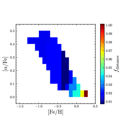
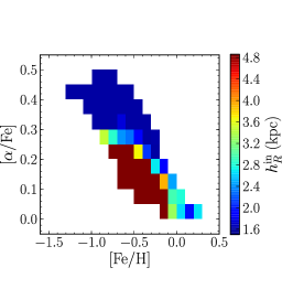
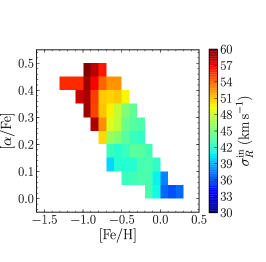
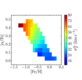
One significant change to the distances that we made for the current analysis is that we have placed the distances on the scale of An et al. (2009), An09 hereafter, which was used in many other analyses of the SEGUE G and K-dwarf samples (e.g., Schlesinger et al., 2012; Zhang et al., 2013), and which appears to provide more accurate distances from the kinematical tests of Schönrich et al. (2012). These distances are typically smaller than the distances calculated using the I08 relation. Because our method for correcting for color and metallicity biases in the sample selection requires a simple photometric distance relation (see 3 and Appendix A below), we apply a single distance factor to the stars in each MAP calculated as the mean distance modulus offset between the I08 and An09 relations for the stars in the MAP, taking into account the MAP’s and distributions (see Figure 1 of BO12d for the difference between the I08 and An09 distance scales as a function of and ). These distance factors are shown in Figure 1. As discussed below, we have checked that our measurements of the surface density as a function of radius are affected by only a few percent by the difference between these two distance scales and are therefore much less sensitive to distance systematics than might be assumed (but we stress that the An09 distances are more accurate and therefore the correct distances to use).
Because dynamical modeling such as that performed in this paper essentially succeeds by finding the gravitational potential that makes the observed velocities consistent with their observed spatial distribution in a dynamical steady state, the detailed understanding of the data sampling function that was crucial for BO12b and BO12d is again an important ingredient for the present analysis. We refer the reader to Appendix A of BO12d for a full description of the SEGUE G-star selection function.
We begin with a SEGUE G-dwarf sample that has about 28,000 stars with acceptably well-determined measurements, but here we only use those 23,767 stars that fall within well-populated ‘mono-abundance’ bins in the (,) plane (BO12d; a bin is well-populated when it contains more than 100 stars; the maximum number of stars in a bin is 789). Furthermore, we exclude MAPs whose best-fit scale length in BO12d was larger than . We exclude these MAPs because their radial profile cannot be well-fit with the simple DF ansatz that we make below. These MAPs are all -poor and have close to solar; they are primarily associated with the outer disk (see Figure 7 in BO12d). This removes 17 MAPs and leaves 16,653 stars in 45 MAPs. For reasons discussed below, we remove 2 MAPs from this sample, such that the final data sample consists of 16,269 stars in 43 MAPs.
3. Analysis method
While stellar dynamics overall is a long- and well-established field (Binney & Tremaine, 2008), the best ways to model large discrete data sets with full phase-space information are still being developed (cf. McMillan & Binney 2012; Rix & Bovy 2013). In what follows, we analyze each MAP separately and independently with the end goal of constraining the total surface density to —, abbreviated as —at a single Galactocentric radius for each MAP. In this and the following Section we describe all of the steps involved in fitting each MAP as a population in a dynamical steady state in order to measure the gravitational potential and how we translate this into a single, robust measurement of at a single radius for each MAP. Our measurements of assume that the rotation curve is flat; if this is not the case, then we show in 4.3 that we still robustly measure the vertical force at .
The basic ingredients of the fitting procedure are:
-
•
Each MAP is fit as a population of stars drawn from a quasi-isothermal DF (; Binney 2010; Binney & McMillan 2011; Ting et al. 2013). This form for the DF has a number of free parameters related to the radial density profile of the tracer population and the radial and vertical velocity dispersions and how they change with . The qDF is described in detail in 3.1.
-
•
The is a function of the orbital actions . For the fit we only need the transformation, which for the disk orbits in our sample can be efficiently, accurately, and precisely computed using a Stäckel approximation of the potential for any reasonable form of the potential near the Galactic plane (Binney, 2012a). This procedure is briefly summarized in 3.1.
-
•
To calculate the orbital actions we require a full 3D model for the Milky Way’s potential. We use a bulge + stellar disk + gas disk + dark halo model that a priori has many free parameters. For the present application we fix at fiducial values all but two of these parameters, the stellar disk scale length and the relative halo-to-disk contribution to the radial force (= circular velocity squared) at . These two parameters are varied to scan through a wide range of , including all a priori reasonable values for the range of Galactocentric radii that we are interested in (). In 4.3 we show explicitly that changing the parameters that are held fixed in the fiducial fit does not significantly impact our measurement of and our measurement of the vertical force at at a single Galactocentric radius is particularly free from systematics. Our model for the Milky Way’s potential is described in detail in 3.2.
-
•
We determine the probability of the position–velocity data (the likelihood) for each set of DF + potential parameters using an expanded version of the methodology described in 3.1 of BO12d, carefully accounting for the sample selection. The calculation of the effective survey volume consists of a nine-dimensional integral, whose fast computation is discussed in Appendix A. We only use the vertical velocity component of the data and marginalize the six-dimensional qDF over the velocity components in the plane, because the planar motions do not constrain the vertical force and they may be affected by non-axisymmetric streaming motions. The fitting procedure is discussed in 3.3.
-
•
For each MAP we determine the full joint PDF for the DF and the potential parameters. By marginalizing this over the DF parameters we obtain constraints on the potential that include uncertainties in the determination of the correct DF. The details on how we explore the PDF are given in 3.4. From the properties of the DF we determine the Galactocentric radius at which is best constrained for each MAP and we calculate and its uncertainty from the PDF. This is described in 4.1.
We now describe these various steps in more detail.
3.1. Distribution function model
We use the quasi-isothermal DF first proposed by Binney (2010) and later refined by Binney & McMillan (2011) to fit the dynamics of a single MAP. BO12 found that the radial and vertical density profiles of individual MAPs are well represented by single exponentials and that the vertical velocity distribution is isothermal, i.e., the vertical velocity dispersion is constant with height above the plane. Further investigation of the Galactocentric radial velocities showed that the radial velocity dispersion is also isothermal (unpublished). As shown in Ting et al. (2013), these properties of MAPs can be reproduced by assuming that the DF is a quasi-isothermal DF of the form of Binney & McMillan (2011). Therefore, in what follows we fit each MAP as a single qDF. This is a simple way of including abundance information to separate different populations into the general approach followed by Binney (2012b), where disk stars with any abundance were fit using a superposition of a large number of qDFs. In the current application, abundances are used to group stars that presumably can be fit using just a single qDF. The requirement that a MAP can be modeled using a single qDF drives our fine-grained pixelization of the (,) plane.
The form for the qDF as it is used here is that of Binney & McMillan (2011)
| (1) |
where is given by
| (2) |
Here , , and are the epicycle, circular, and vertical frequencies (Binney & Tremaine, 2008); is the radius of the circular orbit with angular momentum . We include the factor in equation (2) containing the to eliminate stars on counter-rotating orbits following Binney & McMillan (2011), but we also explicitly set the DF to zero for counter-rotating orbits. , , and are free functions of , which indirectly determine the radial profiles of the tracer density, the radial velocity dispersion, and the vertical dispersion. However, it should be noted that these are merely scale profiles, as opposed to the actual, physical profiles that can be calculated by taking the appropriate moments of the DF. In principle these three functions can take any form, but based on observations of the Milky Way and external galaxies (e.g., Lewis & Freeman 1989; BO12c) we assume that each of these functions is an exponential
| (3) | ||||
| (4) | ||||
| (5) |
To evaluate the qDF for a given position and velocity we need to calculate the actions for that position and velocity, , given . We calculate the actions using the approximate algorithm of Binney (2012a), where the actions are calculated using an (implicit) approximation of the potential as a Stäckel potential. For the sake of a self-contained description, we summarize the relevant parts of the algorithm here. This algorithm proceeds by introducing prolate confocal coordinates
| (6) |
Binney (2012a) discusses how the choice of influences the precision with which the actions are calculated. Based on this discussion, we fix to for all potentials. The momenta in this new coordinate system are given by
| (7) | ||||
| (8) |
If the potential is of the Stäckel form then these momenta are functions of their associated coordinate only
| (9) | ||||
| (10) |
where is the energy and is a constant of the motion (the third integral). This allows one to calculate the actions through a single integration
| (11) |
The crucial ingredient of Binney (2012a)’s algorithm is that although it appears from equations (9-10) that we require an explicit form for and —and thus an explicit representation of the potential in Stäckel form, as in Sanders (2012)—if the potential is close to a Stäckel potential then can be re-written as , where and is a reference value for that does not affect the calculated actions, and similarly can be re-written as . These and can be calculated directly from the potential as
| (12) | ||||
| (13) | ||||
| (14) |
since for a Stäckel potential. If the potential is close to a Stäckel potential, then the dependence of on and that of on is small, so they can be calculated for a chosen reference value of and , respectively.
While we cannot calculate and directly without an explicit representation of the potential in Stäckel form, we can compute the combinations and from the current position and velocity of the orbit (the position and velocity at which the actions are required) if we set to the value corresponding to the given position
| (15) | ||||
| (16) |
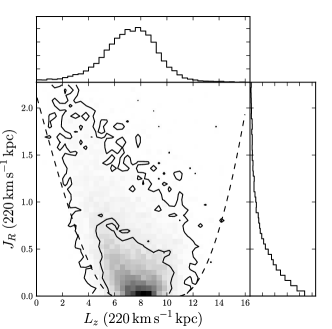
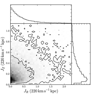
In what follows we always use this algorithm to calculate the actions rather than constructing an interpolation look-up table for a grid of integrals of the motion. The range of the integrals in equations (11) is determined using Brent (1973)’s method for finding the zeros of the integrands and the integrals are then calculated using 10-th order Gauss-Legendre quadrature.
The distribution of the actions of the 16,269 sample stars calculated in a fiducial potential is shown in Figure 2. The diagonal edges in the distribution of and (the radial action and the angular momentum, see below) are due to the fact that circular orbits far from the solar neighborhood (i.e., outside of the bounds of our sample) are not represented in our data set. Similarly, in the distribution of the vertical action , stars with small vertical actions (small vertical energies) are missing in our sample because of the effective lower limit on the vertical height of the stars in our sample; stars with low vertical action do not reach high enough above the plane of the disk to be included in our sample.
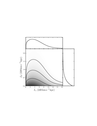
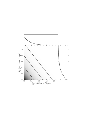
The DF as a function of the actions for a fiducial set of parameters is shown in Figure 3. A comparison between this distribution and the distribution of the data actions in Figure 2 shows that the data’s action distribution is heavily affected by selection biases related to the spatial sampling of the data.
The density, mean velocity, velocity dispersions, etc. of the qDF can be calculated as velocity moments of the 6D qDF:
| (17) | ||||
| (18) | ||||
| (19) |
these can be straightforwardly transformed into the velocity dispersions. In what follows these velocity moments are calculated using 20-th order Gauss-Legendre quadrature between and in the radial velocity , and in the vertical velocity , and and in the rotational velocity ; the dispersions and in these expressions for the ranges are calculated using the scale dispersion profiles from equations (3-5). We use actions calculated using the adiabatic approximation in a few instances below; in this case we use 20-th order Gauss-Legendre quadrature between and , because in the adiabatic approximation the qDF is perfectly symmetric in and separately, which is not the case when using the more correct Stäckel actions (see below).
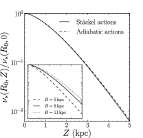
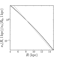
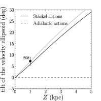
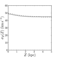
In Figure 4 we show the vertical and radial tracer density profile for a fiducial set of qDF parameters, as well as the tilt of the velocity profile and the vertical velocity dispersion as a function of height. We calculate these using the Stäckel approximation for the actions as well as the simpler, but less precise, adiabatic approximation (e.g.. Binney, 2010). The vertical and radial density profiles are close to exponential, but the vertical profile gradually flattens closer to the plane of the disk. The inset in the leftmost panel shows that the tracer density flares slightly. The right panel shows that the qDF is indeed close to isothermal as the vertical velocity dispersion only increases by a few over ; the same holds for the radial velocity dispersion (see also Ting et al., 2013).
The difference between the Stäckel and adiabatic approximations is small for most observables, except for the tilt of the velocity ellipsoid. The tilt is equal to zero when using the adiabatic approximation because this assumes that vertical and planar motions are close to decoupled, implying that there is no correlation between vertical and radial oscillations along the orbit. The Stäckel approximation does not make this assumption and it correctly captures the correlation between the radial and vertical oscillations for stars that reach large heights above the plane (); the gray line shows the tilt if the velocity ellipsoid is pointing toward the Galactic center and the tilt included in the qDF falls only slightly short of this. Also shown in the third panel of Figure 4 is the measurement of the tilt of the velocity ellipsoid from Siebert et al. (2008), which agrees well with the tilt that results from the qDF if the actions are calculated in the Stäckel approximation.
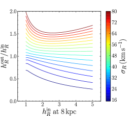
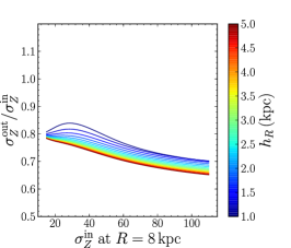
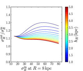
As discussed before, the density and dispersion scale profiles in equations (3-5) are not the physical profiles and the actual density and dispersion profiles as calculated using equations (17) are slightly different. In what follows we use the results from BO12 for the dispersions at to determine a likely range for the qDF parameters for each MAP used in a grid-based exploration of the joint DF–potential PDF. Therefore, we need to determine how the scale profiles relate to the physical profiles. In Figure 5 we show these relations calculated in a potential similar to potential II in Binney & Tremaine (2008). We use this relation to calculate the approximate scale profiles that give physical profiles similar to the best-fit profiles found in BO12 for the radial density and the radial and vertical velocity dispersion at . These estimates are shown in Figure 6.
3.2. Milky Way potential model
While for the present paper we are primarily interested in , the modeling of each MAP using the qDF requires a full 3D model for the Galactic potential. We use a four-component model consisting of a Hernquist bulge with a mass of and a scale radius of 222The details of the bulge model do not matter for the analysis that follows; we use a slightly lower bulge mass than typically found from dynamical considerations, e.g., McMillan (2011), because we use the Hernquist model rather than an exponentially cut-off model as is customary. The rotation curve at , which is the only thing that matters in the analysis below, is similar for our bulge model and that of Binney & Tremaine (2008) and McMillan (2011)., a stellar exponential disk component characterized by a (single, effective) scale height and scale length , a spherical power-law dark halo, and a gas disk modeled as an exponential disk with a local surface density of , a scale height of , and a scale length fixed to be twice that of the stellar disk (following Binney & Tremaine 2008). We do not include a stellar halo component, as the mass of the stellar halo is negligible compared to the other components.
In the qDF fits to data of individual MAPs, the circular velocity curve, the epicycle, and the vertical frequencies are calculated for each potential on a logarithmic grid in between and . The potential is calculated on the same radial grid and on a linear grid in between and . These values are interpolated using two and one-dimensional cubic B-splines and the interpolating functions are used to first calculate the actions for a given and then to evaluate the qDF.
The calculation of the bulge and halo potential and frequencies is straightforward. The potential and forces of an exponential disk with density are calculated using the expressions in Appendix A of Kuijken & Gilmore (1989a), which we repeat here for completeness
| (20) | ||||
| (21) | ||||
| (22) |
and similar expressions for the second derivative of the potential. The integrals in these expressions contain strongly oscillating Bessel functions , especially when evaluating them near the Galactic plane. We calculate these integrals using 10-point Gauss-Legendre integration between each of the zeros of the relevant Bessel function out to ( for the radial force) for and ( for the radial force) for . At large radii () the exponential disk potential is approximated as Keplerian.
The free parameters of the model for the gravitational potential are parameterized using: (1 & 2) the stellar disk mass scale length and mass scale height , (3) the relative contribution of the halo to the stellar-disk+halo contribution to the radial force at , (4) the circular velocity at (this sets the overall amplitude of the potential), and (5) the logarithmic derivative of the circular velocity at with respect to , (i.e., the “flatness” of the rotation curve). All of the other parameters of the potential can be calculated in terms of these basic parameters. We perform all the calculations involving the actions and qDF by first re-scaling the potential such that at ; this requires re-scaling the data positions by and velocities by and re-scaling the input parameters of the qDF similarly. The PDF (see below) then needs to be divided by appropriate factors of and to have the correct units.
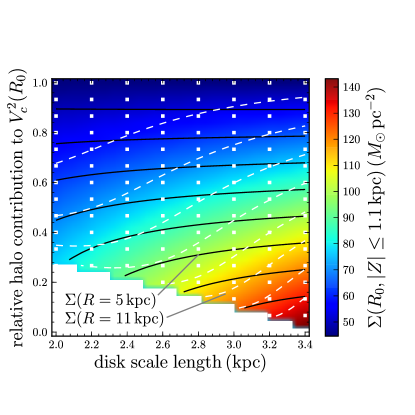
In the fits of a qDF to individual MAPs below we fix all of the five basic parameters except for the stellar disk scale length and the relative halo-to-disk contribution to the radial force at . This proved necessary because exploring the joint qDF+potential parameters PDF for each MAP is computationally expensive such that two potential parameters is the maximum that can currently be efficiently explored (see below for more discussion of this). In our fiducial model we set the stellar disk mass scale height to (this is the mass-weighted mean scale height calculated based on the star-count decomposition of BO12b, i.e., it is the mean of the histogram shown in Figure 2 of BO12b), we fix the potential amplitude to be such that , and we fix the rotation curve to be flat at , i.e., . While these may appear to be strong assumptions, we stress that the main goal of the MAP fits is to measure the surface density at at the Galactocentric radius where this is best determined for each MAP. As such, the range of allowed is what really matters. Figure 7 shows the range of in the fiducial model; it is clear that any reasonable (cf. Bovy & Tremaine 2012; Zhang et al. 2013) is included in the fiducial model. Figure 8 shows the range of between and included in the fiducial model, and this is wide enough to encompass all a priori reasonable . We illustrate below that changing the potential parameters that we keep fixed in the fiducial model does not significantly change our results.
3.3. Fitting procedure
In 3.1 of BO12d we described a method for fitting the density profiles of a sample of stars using the individual positions of the stars in a likelihood-based approach and correcting for the effects of various selection biases. Here we expand this methodology to fitting both the positions and velocities to a 6D DF. As described in 3.1, we model the DF with a dynamical equilibrium model specified by the qDF, which is a function of the actions only, that is . We work in the approximation that the selection function has only a spatial (or magnitude) dependence, which is the case for the G-dwarf sample used in this paper.
We fit a qDF to the various MAPs by taking into account the fact that the observed stellar number counts do not reflect the underlying (volume-complete) stellar distribution, but are instead strongly shaped by (a) the strongly position-dependent selection fraction of stars with spectra (see Figure 11 in BO12d), (b) the need to use photometric distances to relate the underlying phase-space model to the observed magnitude distribution (as the magnitude-limited SEGUE sample corresponds to a color- and metallicity-dependent distance-limited sample), and (c) the pencil-beam nature of the survey. As in BO12d, we model the observed distribution of stars as a Poisson sampling of the underlying population. The details of this method are the same as that described in 3.1 of BO12d and we refer the reader to that paper for a detailed discussion.
Since the photometric distance estimates depend on the color, metallicity , and apparent -band magnitude, and because the selection function is a function of position, , and , we need to model the observed density of stars in color–magnitude–metallicity–phase (position–velocity) space, . This density of stars can be written as
| (23) |
Here, are Galactocentric cylindrical coordinates corresponding to rectangular coordinates , which can be calculated from . The factor is the number density in magnitude–color–metallicity space as a function of position (see further discussion in Appendix B of BO12d). The is a Jacobian term because of the coordinate transformation; the factor is the selection function as given in equation (A2) of BO12d. Finally, is the underlying DF of the sample. While we model this DF as being a function of the actions only, we stress that the DF always remains a density in –space333This caveat may seem unnecessary as the Jacobian of the canonical transformation is unity. However, because we cannot calculate the actions exactly, the Jacobian will not be exactly equal to one.. The parameters of the gravitational potential enter the observed density through the dependence of on . We denote the parameters of the DF using .
The likelihood of a given model for the DF and potential is given by that of a Poisson process with rate parameter . After marginalizing over the amplitude of the DF with a logarithmically-flat prior (which effectively normalizes the DF), the likelihood of a single data point given by
| (24) |
The second term normalizes the density over the observed volume. In Appendix A we describe how we calculate the 9-dimensional normalization integral efficiently. For comparison with observed velocities, we convolve the likelihood in equation (24) with the observational velocity uncertainties.
Because we are primarily interested in measuring the surface density , the dynamics of MAPs in the plane of the Milky Way is mostly irrelevant as it does not contain much information about the vertical surface density. Moreover, non-axisymmetric perturbations to the Galactic potential (e.g., those from spiral structure or the bar) strongly affect the kinematics in the plane of the Galaxy, such that non-axisymmetric planar kinematics ( and ) could bias the fit of an axisymmetric model to the MAP data. Practically, discarding the planar kinematics also allows us to fix the parameters of the qDF related to the radial velocity dispersion, as they only affect the distribution of velocities in the plane; this reduces the number of qDF parameters from five to three, thus significantly reducing the computations involved in evaluating the likelihood (see 3.4 below). Therefore, we do not consider the planar kinematics and marginalize the likelihood over and for each star. Thus, we only need to convolve the likelihood with the observational uncertainty in the vertical velocity (since we assume that distance uncertainties are only important as far as the velocity is concerned). We perform this convolution using 20-th order Gauss-Legendre quadrature over the range , where and are the observed velocity and its uncertainty. Thus, the likelihood for a single data point becomes
| (25) |
We also add an outlier model consisting of a constant spatial density and a Gaussian velocity distribution with a dispersion of ; for MAPs with best-fit scale heights from BO12d larger than 500 pc, this outlier velocity dispersion is multiplied by two. This outlier model mimics a halo population. The outlier fraction is added as a free parameter. In the analysis below, the outlier fraction is small for most MAPs; only the most -old, -poor MAPs have outlier fractions of , because their intrinsic dispersions are large. Most importantly, there is no correlation between the outlier fraction and the inferred value of , such that it does not affect our results. The full likelihood is then given by
| (26) |
where is the likelihood contribution from the outlier model.
3.4. Further implementation details
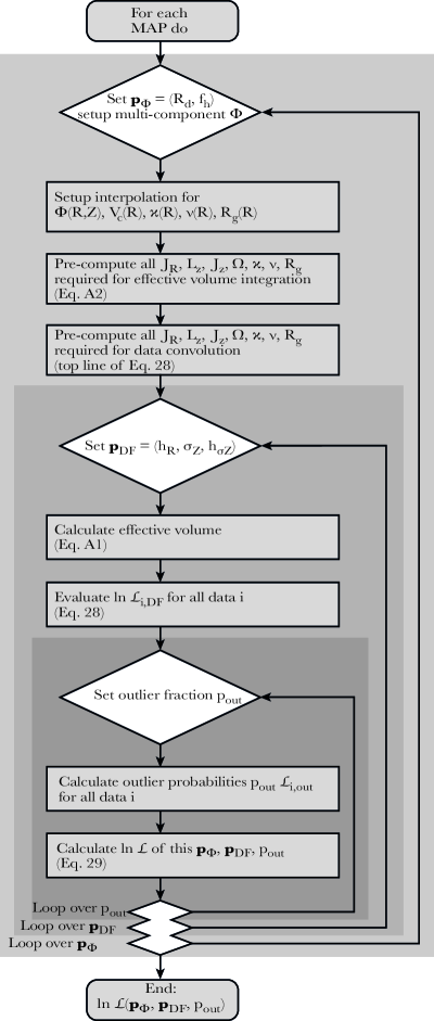
Using the methodology described in the previous Section, we explore the joint PDF of the potential and qDF parameters for each MAP separately. We do this by calculating the PDF on a fixed grid specified below. This Section gives the details of the specific implementation choices made to explore the joint PDF of potential and qDF parameters in a computationally efficient manner. The main steps of the implementation are shown graphically in Figure 9.
| fiducial model | 8 values from to | 16 values from to | |||
| systematics: high | 8 values from to | 16 values from to | |||
| systematics: low | 8 values from to | 16 values from to | |||
| systematics: low | 8 values from to | 16 values from to | |||
| systematics: falling rot. curve | 8 values from to | 16 values from to | |||
| systematics: rising rot. curve | 8 values from to | 16 values from to |
The potential grid consists of 8 stellar disk scale lengths ranging from to and 16 relative halo-to-disk contributions to , ranging from to . We do not consider models in which the halo power-law is smaller than 0 or larger than 3; these regions are blank in Figure 7. The list of potential parameters, the range over which the two basic parameters are varied, and the values at which the other potential parameters are fixed are given in Table 2 for all of the potential models considered below.
| Parameter | Range considered |
|---|---|
| 8 values log.-spaced between and | |
| 16 values log.-spaced over range of width 0.36 around estimate in Figure 6 | |
| 8 values log.-spaced between and | |
| fixed at estimate in Figure 6 | |
| fixed at |
The qDF as described in 3.1 has nominally five free parameters. However, as discussed in the previous Section, we marginalize the likelihood over the radial and azimuthal velocity components and , such that the parameters describing the radial dispersion profile— and —are not important for the data modeling. Therefore, we fix at the values estimated based on fits of the radial dispersion similar to those performed in BO12c (see Figure 6) and we set . This leaves three free qDF parameters for each MAP: , , and . Table 4 lists all five qDF parameters and the range over which they are varied in the analysis, as described below.
For each MAP we consider the same range of : 8 values from to . The range of the vertical dispersion scale length is also the same for each MAP: 8 values logarithmically spaced between and . The range of is set individually for each MAP based on the estimates for from Figure 6. 16 values are logarithmically spaced over a range of width around the estimated . The central values were slightly adjusted based on visual inspection of the PDFs such that the best-fit does not occur at the edge of the parameter range; these adjustments are typically less than .
In practice, for computational speed reasons, the likelihood calculation is structured as shown in Figure 9. We first setup an interpolation grid for the potential and the rotational, epicycle, and vertical frequencies as well as the guiding-star radii. These grids are then used to quickly evaluate the gravitational potential when calculating the actions and the interpolated frequencies and guiding-star radii are used in the fast evaluation of the qDF (see below). This step is necessary because directly evaluating the contribution to the potential coming from the stellar and gas exponential disks would be prohibitively computationally expensive. The explored parameters for each MAP are then separated in three classes: (1) the potential parameters , (2) the 3 qDF parameters, and (3) the outlier fraction.
Once the parameters of the potential are specified, all of the actions that are involved in evaluating the likelihood in equation (25) are pre-computed. This includes all of the actions involved in the calculation of the effective survey volume (equation [A2]) and the actions for the data that are used to convolve the likelihood with the vertical velocity uncertainty (equation [25]). As discussed above, these integrals over the velocities are performed over a range specified by the model dispersions (those that are explicit parameters of the qDF). In order to be able to re-use the actions for multiple qDF parameter sets, we calculate the integrals over the velocity, always using ranges based on the estimated dispersions from Figure 6. As the dispersions that are considered during the PDF exploration are typically within of these estimates and we integrate out to , this procedure works well for all of the considered qDF parameters. It also makes sure that there is no stochastic noise in the likelihood evaluation, which could be large if the velocity and/or spatial integrals are performed using Monte Carlo integration (see discussion in McMillan & Binney 2013 and Ting et al. 2013). We also pre-calculate the rotational, epicycle, and vertical frequencies as well as the guiding star radii associated with all of the points at which the qDF has to be evaluated in the course of a single likelihood evaluation (cf. the definition of the qDF in equation [1]). Once the actions, frequencies, and guiding star radii are calculated, the likelihood can be quickly evaluated for different sets of qDF parameters, by evaluating the qDF using the pre-calculated values and re-summing the integrals.
With all of the actions etc. pre-calculated we then vary the qDF parameters (second loop in Figure 9). For any given qDF parameter set we calculate the effective survey volume and evaluate the likelihood related to the qDF for all of the data points. The outlier fraction can then be varied very quickly and we use a grid of 25 outlier fractions ranging from to (innermost loop in Figure 9).
We find that by using Gauss-Legendre quadrature to perform the velocity integrals, we can evaluate the effective survey volume accurately enough (that is, to an accuracy , sufficiently small such that this is not a source of noise in the likelihood) using action evaluations. This is less than the evaluations required by McMillan & Binney (2013) and this leads to a significant reduction in the time required for a single likelihood evaluation, as setting up the grid of actions takes up a significant amount of time. The reason Gauss-Legendre quadrature works well is that the qDF is a very smooth function and it is easy to estimate the range over which it is non-zero. Similarly, we have found that Gauss-Legendre quadrature is far superior to Monte Carlo sampling for convolving the likelihood with the velocity uncertainty: we can accurately calculate the convolved likelihood with 20-th order Gauss-Legendre quadrature, whereas when even using thousands of Monte Carlo samples the convolution was not well-behaved (even though we used the same Monte Carlo samples for all different parameter settings, to remove numerical noise as advocated in Ting et al. 2013). Future analyses of Gaia data will still be mostly in the regime where distance uncertainties are only important through their influence on the velocity uncertainties. As 3D Gauss-Legendre quadrature could be adequately performed using evaluations of the integrand, Gauss-Legendre quadrature will likely still be superior to Monte Carlo integration.
The computational time is dominated both by setting up the grid of actions and frequencies for a given potential and calculating the effective survey volume for a given set of qDF parameters. Using all of the speed-ups described in this Section, the exploration of the PDF still requires using 8 cpus for a single MAP. Each MAP’s PDF can be explored independently and all of the steps involved in the likelihood evaluation can be easily parallelized such that the availability of sufficient computational resources is the main limitation for exploring a wider range of potential models. The combined computational cost for all steps of the analysis described in this paper was cpu-hours, or cpu-hour per datapoint.
4. Results
In this Section we present the results of fitting each MAP with a qDF model to measure at the Galactocentric radius at which this quantity is best constrained for each MAP. In 4.1 we discuss the joint constraints on the dynamical parameters of the gravitational potential model and on the qDF parameters for each MAP individually. We then describe how we determine the radius for each MAP at which is best constrained for that MAP. In 4.2 we present the profile that results from combining the individual fits to the different MAPs. In 4.3 we show that the profile that we measure using the fiducial model for the gravitational potential does not significantly change if we change the parameters of the fiducial potential. We also demonstrate that the impact of systematic distance uncertainties is small.
4.1. Results for individual MAPs and determination of
As discussed in 3, we fit each set of MAP data using a qDF model and we determine the joint PDF of two dynamical parameters + three qDF parameters on a grid in all of the parameters. We thus obtain constraints on the basic dynamical parameters, disk scale length and relative halo-to-disk contribution to , after marginalizing over the parameters of the qDF (which is a weak form of the “summing over all possible DFs” of Margorrian (2006)). We can calculate the PDF of derived dynamical parameters, such as the surface density at a given radius, the density of the dark halo, etc., by appropriate transformations of the PDF of the basic dynamical parameters (with the understanding that all of the different derived parameters will be strongly correlated because there are only two free parameters). Similarly, we can marginalize over the dynamical parameters to constrain the qDF parameters for the individual MAPs, but this is not the focus of this paper.
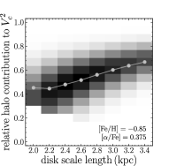
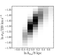
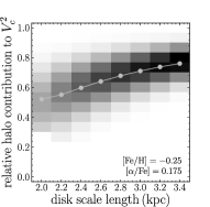
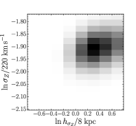
Figure 10 shows as examples the PDFs resulting from the fits to two MAPs for the basic dynamical parameters as well as PDFs for the qDF parameters related to the vertical velocity dispersion, and . We only show PDFs for two MAPs in Figure 10 and we only show two different 2D marginalized PDFs to give a sense of the PDFs and how they are different for metal-poor and metal-rich MAPs. We have visually inspected all such PDFs as well as other 2D projections for all individual MAPs. We have done this for the fit of the fiducial potential model as well as for all of the systematics checks in 4.3. All PDFs were found to be sensible, although in a few cases the range of had to be changed and the PDF had to be re-computed since the best-fitting value of was found to lie on the boundary of the grid. Only for one of the 45 MAPs in our initial sample were we unable to adjust the range of within an acceptably small number of iterations and we dropped this bin from further consideration: this MAP is located at , , and it contained only 129 data points.
To assess whether the qDF model is a good fit to the observed spatial density and kinematics of the MAPs we have performed extensive direct comparisons between the data and the best-fitting model for each MAP. We do this by projecting the best-fitting model into the space of observables taking into account the various selection biases affecting the data. These data–model comparisons are described and discussed in detail in Appendix B. Overall, we find that the spatial distribution and the vertical kinematics of the data are very well fit by the qDF models for individual MAPs. However, we remove from further consideration the MAP at and , because the detailed comparisons between the data and the model indicates that no good fit is obtained for this MAP; this MAP contains 255 data points. All 43 other MAPs, containing 16,269 data points, are included in the results described below.
In principle, the optimal way of constraining the mass distribution using individual MAPs would be to multiply together the individual PDFs for the dynamical parameters. However, these PDFs of the individual MAPs are not mutually consistent, e.g., the joint PDF for all -old MAPs is inconsistent with the joint PDF for all metal-rich, -young MAPs. This is a reflection of the fact that our fiducial model for the gravitational potential, with only two free parameters, is too restrictive, i.e., it does not contain a model that is consistent with all of the individual MAPs. However, the 2-parameter potential model is general enough to provide a measurement of the gravitational force in the small range of radii for each MAP that most affects the MAP’s orbital distribution.
The PDF of the dynamical parameters in Figure 10 and those of all other MAPs are characterized by a strong degeneracy between the two basic dynamical parameters. A comparison with Figure 7 shows that this degeneracy is along lines of constant surface density, which is expected as the vertical kinematics of an individual MAP primarily constrains the total surface density. A comparison with Figure 7 also makes it clear that the direction of the degeneracy is indicative of the radius at which the surface density is best constrained by the data of an individual MAP. We focus on the surface density at a height of , because that is close to the mode of the distribution of distances-from-the-midplane of the data for each MAP, which is set through the combination of the intrinsic vertical distribution and the SEGUE selection procedure.
Formally, we can calculate the radius at which is best determined by calculating the correlation between the disk scale length and as a function of and finding the radius at which this correlation is minimized. This radius serves as the point around which pivots as the model’s scale length is changed. As such, it is the radius at which is most robustly determined. From the PDF of the dynamical parameters, we can then calculate the mean and its uncertainty at that radius. Figure 11 illustrates this procedure.
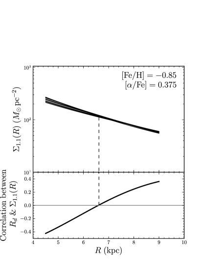
Figure 10 shows that the degeneracy in the PDF of the dynamical parameters, and therefore the correlation between and the disk scale length, is different for different MAPs. Thus, the radius at which is best determined is different for the various MAPs. This is plausible as stars of a given MAP, found in the Solar vicinity, are drawn from tracer populations of very different scale lengths (BO12d). We expect that MAPs with abundances that are close to solar measure at a radius that is close to the solar circle, because these stars dominate the local population of stars and they spend much of their orbits close to the solar circle. Likewise, we expect that the -old MAPs, which have short scale lengths and large velocity dispersion (BO12), spend a much larger fraction of their orbit at smaller radii and therefore measure closer to the Galactic center.
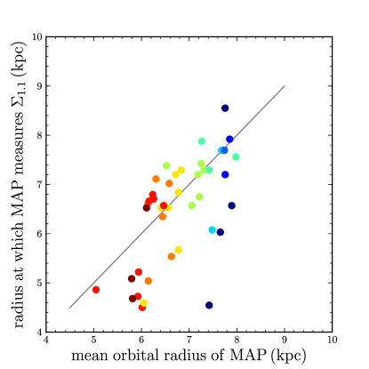
To test whether this expectation is borne out in practice, and therefore, whether the procedure of determining the radius at which is best measured makes sense, we have calculated the median of the mean orbital radii of the data in each MAP. We use a simplified model for the Milky Way’s gravitational potential that is the same as that used in Sec. 5.4 and Figure 7 of BO12d, but the details of the mass model for the Milky Way used are unimportant for the calculation of the mean orbital radii. As we are interested in the vertical dynamics, we time-average over the orbits weighting by the midplane density ( vertical oscillation frequency squared). These median mean-orbital-radii for each MAP are plotted against the radii with the most robust determination in Figure 12, color-coded by .
It is clear from Figure 12 that there is a strong correlation between the radii calculated in these two entirely different manners (apart from a single outlier in the lower-right corner). Therefore, we can be confident that the procedure for calculating the radius at which each MAP best measures provides a good definition for this radius. The color-coding confirms the expectation that -old MAPs constrain at radii much smaller than , while -young MAPs measure at positions close to the Sun’s. MAPs that are intermediate between these two measure at intermediate radii. One of the more -young MAPs in Figure 12 falls far from the relation defined by the other MAPs (best radius of for a mean orbital radius of ). However, this single MAP does not influence any of the results obtained below. Below, we quote results using the best radius as determined from the PDF; if we instead require the measurements of the vertical force to be at the median of the mean orbital radii of the stars in each MAP, the best-fit surface-density and vertical-force profiles are unchanged, albeit with slightly increased uncertainties on the scale lengths.
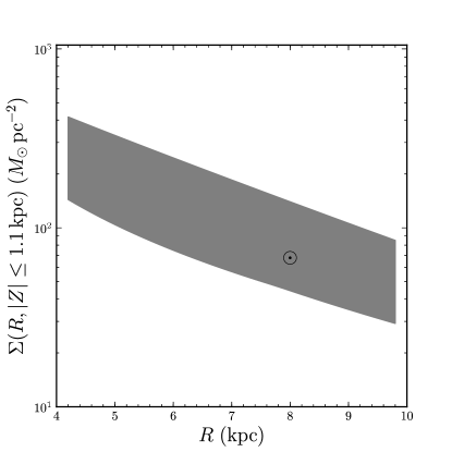
4.2. The surface density at 1.1 kpc between 4 kpc and 9 kpc as measured by MAPs
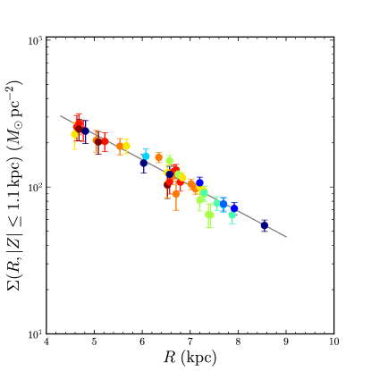
Even though the data from the different MAPs were sampled by the same survey centered on the solar radius (see Figure 7 in Rix & Bovy 2013), they constrain at quite different radii. As a consequence, we can measure the Galactic disk’s surface density profile. For each MAP we calculate the mean and its uncertainty at the best radius from moments of the PDF of the dynamical parameters. Thus, we condense each MAP’s dynamical information into the best single measurement of the Milky Way’s mass distribution for that MAP. The surface densities thus measured are shown in Figure 13 and tabulated in Table 6.
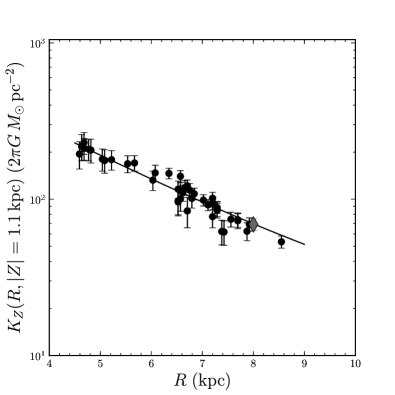
Figure 13 shows that the MAPs provide a highly precise measurement of between and and that the results from all 43 MAPs are in excellent agreement with each other. From a purely phenomenological perspective this measurement of can be well-characterized by a single exponential
| (27) |
with formal uncertainties of in the normalization and in the scale length. However, we have no reason to expect that the real physical is a single exponential, as the mass distribution is made up of various disk components and the halo. We discuss this further in 5 below, where we fit mass models.
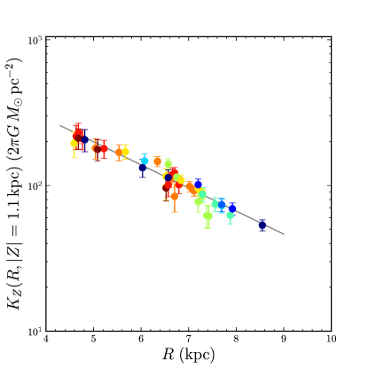
An alternative way of presenting our results is as measurements of the vertical force at , which we denote by , instead. These measurements are shown in Figure 14 and are also tabulated in Table 6. As with the measurements of , the radial dependence of the vertical force is well-fit by an exponential as
| (28) |
again with formal uncertainties of in the normalization and in the scale length. As expected based on the vertical Jeans equation and shown explicitly in the following Section, our measurements are more robust with respect to changes in the assumptions about the derivative of the circular velocity (i.e., the “slope of the rotation curve”). Therefore, when using our measurements to constrain dynamical models of the Milky Way, it may be preferable to use the measurements rather than the , especially when considering models where the rotation curve is significantly non-flat. This is the approach we follow in 5 below.
We have assumed throughout the analysis. The effect of changing is to shift our measurements of and such as to keep constant (i.e., our measurements are at a fixed distance from ; see also 4.3). Therefore, our measurements can be shifted to a different value of by keeping (see Table 6) constant.
The measured or in Figures 13 and 14 and tabulated in Table 6 are 43 new, independent constraints on the Milky Way’s mass distribution and gravitational potential. They can be combined with other constraints, such as measurements of the vertical mass distribution as in Bovy & Tremaine (2012) and Zhang et al. (2013), and constraints on the rotation curve from the terminal velocity curve or based on stellar tracers. This is the approach that we take in 5, where we show that the MAP measurements of quite directly constrain the disk scale length and through combination with data on the rotation curve can be used to disentangle the disk- and halo contributions to the mass distribution in the inner Milky Way.
| (dex) | (dex) | (kpc) | () | () | (kpc) | () | () |
|---|---|---|---|---|---|---|---|
| -1.25 | 0.425 | 4.63 | 256.0 | 50.4 | 3.37 | 217.6 | 41.5 |
| -1.15 | 0.425 | 4.68 | 270.9 | 44.3 | 3.32 | 230.6 | 36.8 |
| -1.05 | 0.375 | 6.71 | 89.7 | 20.3 | 1.29 | 84.2 | 18.5 |
| -1.05 | 0.425 | 4.77 | 244.2 | 40.1 | 3.23 | 209.0 | 33.2 |
| -0.95 | 0.325 | 4.59 | 228.4 | 48.3 | 3.41 | 194.7 | 38.6 |
| -0.95 | 0.375 | 5.04 | 207.6 | 34.9 | 2.96 | 180.5 | 29.2 |
| -0.95 | 0.425 | 5.22 | 204.3 | 30.1 | 2.78 | 179.0 | 25.6 |
| -0.95 | 0.475 | 4.68 | 247.9 | 41.3 | 3.32 | 211.4 | 33.7 |
| -0.85 | 0.275 | 7.38 | 65.0 | 11.9 | 0.62 | 62.2 | 11.2 |
| -0.85 | 0.325 | 6.53 | 104.9 | 19.8 | 1.47 | 97.5 | 18.0 |
| -0.85 | 0.375 | 6.62 | 118.1 | 14.0 | 1.38 | 109.8 | 12.9 |
| -0.85 | 0.425 | 6.66 | 127.6 | 14.0 | 1.34 | 119.0 | 12.9 |
| -0.85 | 0.475 | 5.08 | 202.8 | 35.9 | 2.92 | 176.8 | 30.1 |
| -0.75 | 0.275 | 7.42 | 64.4 | 11.6 | 0.58 | 61.7 | 11.0 |
| -0.75 | 0.325 | 6.53 | 125.0 | 16.2 | 1.47 | 115.9 | 14.8 |
| -0.75 | 0.375 | 7.11 | 97.3 | 8.0 | 0.89 | 92.0 | 7.5 |
| -0.75 | 0.425 | 6.71 | 130.6 | 11.8 | 1.29 | 121.9 | 10.9 |
| -0.75 | 0.475 | 6.53 | 103.3 | 19.8 | 1.47 | 96.1 | 18.0 |
| -0.65 | 0.275 | 7.20 | 81.4 | 12.6 | 0.80 | 77.3 | 11.8 |
| -0.65 | 0.325 | 7.20 | 100.2 | 9.9 | 0.80 | 95.2 | 9.3 |
| -0.65 | 0.375 | 6.34 | 159.2 | 12.7 | 1.66 | 146.3 | 11.5 |
| -0.65 | 0.425 | 6.79 | 108.0 | 14.5 | 1.21 | 101.2 | 13.4 |
| -0.55 | 0.275 | 7.29 | 89.2 | 9.6 | 0.71 | 84.9 | 9.1 |
| -0.55 | 0.325 | 7.29 | 93.1 | 7.8 | 0.71 | 88.5 | 7.4 |
| -0.55 | 0.375 | 7.02 | 104.7 | 8.7 | 0.98 | 98.7 | 8.2 |
| -0.55 | 0.425 | 6.57 | 108.3 | 18.7 | 1.43 | 100.8 | 17.1 |
| -0.45 | 0.225 | 7.56 | 77.6 | 8.5 | 0.44 | 74.5 | 8.1 |
| -0.45 | 0.275 | 6.75 | 122.4 | 12.6 | 1.25 | 114.3 | 11.7 |
| -0.45 | 0.325 | 6.84 | 115.7 | 10.1 | 1.16 | 108.4 | 9.4 |
| -0.45 | 0.375 | 5.54 | 189.6 | 24.1 | 2.46 | 168.6 | 20.9 |
| -0.35 | 0.225 | 7.29 | 91.5 | 10.2 | 0.71 | 87.2 | 9.6 |
| -0.35 | 0.275 | 6.57 | 150.9 | 13.5 | 1.43 | 140.1 | 12.4 |
| -0.35 | 0.325 | 5.67 | 190.6 | 22.3 | 2.33 | 170.6 | 19.5 |
| -0.25 | 0.175 | 7.70 | 75.6 | 8.4 | 0.30 | 72.8 | 8.0 |
| -0.25 | 0.225 | 7.88 | 64.6 | 8.5 | 0.12 | 62.4 | 8.2 |
| -0.15 | 0.125 | 7.70 | 76.7 | 8.1 | 0.30 | 73.9 | 7.8 |
| -0.15 | 0.175 | 6.08 | 161.8 | 19.8 | 1.92 | 147.4 | 17.7 |
| -0.05 | 0.025 | 6.57 | 121.9 | 16.4 | 1.43 | 113.2 | 14.9 |
| -0.05 | 0.075 | 7.92 | 71.4 | 7.0 | 0.08 | 69.2 | 6.8 |
| 0.05 | 0.025 | 8.55 | 54.7 | 4.9 | -0.55 | 53.4 | 4.7 |
| 0.05 | 0.075 | 7.20 | 106.8 | 10.0 | 0.80 | 101.3 | 9.4 |
| 0.15 | 0.025 | 6.03 | 145.4 | 20.9 | 1.97 | 132.4 | 18.8 |
| 0.25 | 0.025 | 4.82 | 240.3 | 42.9 | 3.18 | 206.2 | 35.7 |
Note. — Each row gives the measurement of the surface density up to along with its uncertainty obtained from a single MAP, specified by its central and . The radius is that where the correlation between the inferred surface density and the potential model’s disk scale length is minimal; this is the radius at which the surface density is best measured by a MAP (see Figure 11). The last two columns give the alternative measurement of the vertical force at and its uncertainty . The sixth column gives the difference between the radius at which or is measured and (to be held constant when using our measurements with a different value of ).
4.3. Variations on the fiducial model
The results in the previous Section are obtained in the fiducial model in which we use the An09 distance scale for the G-type SDSS dwarfs and we fix the parameters of the gravitational potential model such that , , and . In this Section we determine the impact of these choices and find them to be small and largely inconsequential for the measurement of and especially , and for the dynamical analysis in 5 below.
We assess the impact of systematic distance uncertainties by performing the analysis of the MAP dynamics when using the distances of I08 instead of the An09 distances in our fiducial model. As discussed in 2, the I08 distances are typically larger than the An09 distances to G-type dwarfs, with the detailed relative distance factors given in Figure 1. As discussed in BO12d, the impact of unresolved binaries is such that distances would be larger, so the difference between the results obtained using I08 distances and those derived from An09 is a good proxy for understanding the impact of typical systematic distance uncertainties affecting the data.
We expect the impact of systematic distance uncertainties to be such that , with and similar for . This is because roughly , such that if the measurement is dominated by proper motions, such as when one observes the vertical motions of disk stars far from the Sun, . Similarly, if the measurement primarily depends on the line-of-sight velocities, which is the case when measuring at by looking at the motions of stars near the Galactic poles, . Because the measurement of has contributions from both proper motions and line-of-sight velocities, we expect to scale with distance in a manner that is in between these two extremes. We expect the scaling to be different for different MAPs, as MAPs that measure at smaller rely more on proper motions than MAPs that measure closer to the solar circle.
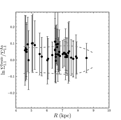
We show the comparison between the measured obtained using the I08 distances with those derived from the An09 distances in Figure 15. The difference in the measured is shown for each MAP at the radius at which the MAP best measures determined for the fiducial model. The dashed lines show the approximate locus of the linear and inverse scalings with distance discussed in the previous paragraph. This Figure shows that the impact of the systematic distance shift between the two distance scales is small for the majority of the MAPs. MAPs that measure at rely more on proper motions and their measured therefore scales close to linear with the distance scale. Most of the MAPs that measure at are only affected at the few percent level by the uncertainty in the distance scale. is affected in the same way as .
The overall impact of the change in the distance scale between that of I08 and An09 on is small. It is clear from Figure 15 that the effect of using the larger distances is to slightly steepen the profile. The best-fit exponential approximations to and obtained using the I08 scale, using the optimal radii derived from the PDFs for the I08 scale are
| (29) | ||||
| (30) |
which is very close and within the statistical uncertainties of the result obtained using the An09 scale (equation [27]). Therefore, the impact of systematic distance uncertainties on the measurement of and is insignificant, at the level of .
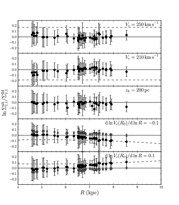
To determine the impact of the rather constrained fiducial model for the gravitational potential, we repeat the measurement of for different choices for the most important fixed parameters of the potential. Foremost among these is the normalization of the potential, characterized by the local circular velocity in our parameterization. We have fixed this to in the fiducial model. In the top panel of Figure 16 we compare the results when using to those obtained for the fiducial model, again at the radius determined using the fiducial model. We see that the impact of changing the potential normalization is close to zero for almost all MAPs and in all cases the shift is much smaller than the random uncertainties. The dashed line in this figure shows the expected difference if , the expected scaling if the measured surface-density were wholly dependent on the normalization of the potential (or equivalently, of the rotation curve), that is, if we were not really measuring or . behaves the same when changing . Similarly, in the second panel we compare the results obtained using to those from the fiducial model; these two sets of results are again nearly indistinguishable and the difference is much smaller than the expectation (dashed line). Note in this case that the measured value for for the bins that measure at is at the edge of the prior range for , which artificially lowers the inferred for these MAPs (this is clear from an inspection of the PDFs). The best-fitting exponential approximations to and measured from the results are
| (31) | ||||
| (32) |
and those from the results are
| (33) | ||||
| (34) |
Therefore, the scale length of hardly changes and the normalization is only affected by a few percent, which is similar to the statistical uncertainties in the fit.
We have also performed an extreme test where we set , far beyond any reasonable setting for this parameter. Setting to shifts the prior on in Figure 8 upward such that many of the best-fit in Figure 13 lie on the edge or slightly outside the prior range. We find that the measured for are all on the lower edge of the prior, such that they clearly indicate that is in reality lower than what is allowed by the prior. Even in this extreme case (which should not be trusted, since all measured are on the edge of the prior), the scale length of the best-fitting exponential is and the normalization only changes to . This change in normalization is only , while has changed by . This and the results for and confirm that we are primarily measuring (or ) such that the assumed normalization of the potential is unimportant as long as it permits the inclusion of the actual .
In the fiducial model, the scale height of the stellar disk is fixed to , which is the mass-weighted scale height inferred from the MAP decomposition of BO12 and agrees with dynamical measurements of the disk scale height based on (Siebert et al., 2003; Zhang et al., 2013). However, the mass-weighted scale height of the disk is still quite uncertain. Because we are primarily measuring using the vertical kinematics, we do not expect our results to depend on the disk scale height, which for any reasonable value changes the vertical distribution of disk matter below approximately , but not above it (as at most a few disk are above ). We have repeated the analysis above using a scale height of , which is at the low end of plausible values of this parameter. The middle panel of Figure 16 demonstrates that the inferred for all MAPs barely change when using a different stellar-disk scale height, and all changes are within the random uncertainties of the measurement. The inferred and are almost exactly the same as those measured using the fiducial potential model:
| (35) |
and
| (36) |
The final important parameter of the gravitational-potential model is the slope of the rotation curve, set to in the fiducial model. From the vertical Poisson equation it is clear that the slope of the rotation curve changes the surface density measured from vertical kinematics by adding approximately (Kuijken & Gilmore, 1989a; Bovy & Tremaine, 2012). Locally this amounts to a systematic uncertainty of
given the current uncertainty in the slope of the rotation curve (see below). However, we expect the vertical force to be unaffected by this, because the vertical Jeans equation shows that is constrained by the vertical dynamics only and that it does not depend on the slope of the rotation curve.
The bottom two panels of Figure 16 show the change in the measured and (gray diamond symbols) when changing the assumed slope of the rotation curve. This changes the slope of the model rotation curve at all and the dashed lines show the expectation from the simple calculation given in the previous paragraph assuming that the change is such that at all . It is clear that the measurements of are strongly and systematically affected by the change in the slope of the rotation curve, especially near . The inferred profile changes by about twice the random uncertainties:
| (37) | ||||
| (38) |
However, the measured is much less affected by the change in the slope of the rotation curve and the change in is well within the random uncertainties for all MAPs. The inferred profile changes only by about :
| (39) | ||||
| (40) |
Therefore, the inferred are more robust to changes in the assumed rotation curve. When using our measurements in analyses where the rotation curve is varied or assumed to be very different from the flat rotation curve in our fiducial model, we recommend using the measurements instead of the measurements.
We have also investigated the effect of changing the value of . One would expect that our measurements, which are based on a volume centered on the Sun, are at constant distances from the assumed . Therefore, we should find that a measurement of or at for is at , where , for a different value of . We have performed the full measurement for the two MAPs in Figure 10 using and have found that the inferred and is indeed shifted by for these MAPs, such that their measured and are the same as for the fiducial , but at Galactocentric radii that are larger. We are therefore confident that this holds for the measurements from all of the MAPs. Table 6 contains a column that lists the radius at which and is measured; this value should be kept constant when changing the assumed value of .
The effect of changing is only to shift the measured and profiles without changing their (logarithmic) slopes. Below, we are primarily interested in determining the mass scale length of the stellar disk and this measurement is mainly dependent on the logarithmic slope of the surface density profile. As this slope does not depend on the assumed value of , we do not vary in the analysis below.
5. Measurement of the disk scale length and constraints on the mass profile in the inner Milky Way
The measurement of the vertical force profile between and presented in the previous Section provides a strong new constraint on mass models for the inner Milky Way. We explore these constraints in this Section. We find that the stellar disk scale length is largely constrained by the measurements of , but we also consider additional data on the rotation curve and the local vertical mass distribution to separate the disk and halo contributions to the total mass. These additional data are described in 5.1. The results of mass-model fits to these data are presented in 5.2.
5.1. Additional data
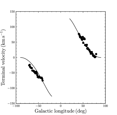
As additional constraints on the mass distribution in the inner Milky Way, we use data on the rotation curve and the vertical mass distribution near the Sun. The rotation-curve data that we use are in the form of terminal velocities measured through HI and CO emission. In the fourth quadrant we use the HI data from McClure-Griffiths & Dickey (2007) and in the first quadrant we use the CO data from Clemens (1985), both binned into bins of . These terminal velocity measurements are shown in the bottom panel of Figure 17. Because the terminal velocities are characterized by wiggles on the order of that are likely due to the effects of non-axisymmetry, we model these data very conservatively by assuming that they have an uncertainty of correlated over . This makes sure that wiggles typical of non-axisymmetry do not affect our results. Because the terminal velocities depend on the Sun’s peculiar velocity in the plane of the Milky Way through terms proportional to and , we further marginalize over such terms in the fits below, so that any effects of non-axisymmetry and the Sun’s peculiar velocity do not affect the analysis.
We further use constraints on the local slope of the rotation curve. Such constraints exists, e.g., from the measurement of the Oort constants (e.g., Feast & Whitelock, 1997), from the kinematics of masers in the disk of the Milky Way (Reid et al., 2009; Bovy et al., 2009), or from the kinematics of stars throughout the disk (Bovy et al., 2012a). Since the measurement of of Bovy et al. (2012a) encompasses the results from these different analyses, we use it to represent the current uncertainty in the logarithmic slope of the rotation curve. We represent the Bovy et al. (2012a) measurement with the simple analytic form
| (41) | ||||
which approximately matches the PDF for of Bovy et al. (2012a). We stress that we do not use any measurements of the circular velocity itself. This way we can assess what direct measurements of the mass distribution combined with measurements of the shape of the rotation curve (but not its normalization) constrain the circular velocity to be.
Finally, we also include measurements of the vertical mass distribution near the Sun, . A number of such measurements exist in the literature and we use the results from Zhang et al. (2013), which are the best measurements of to date and they are consistent with all other measurements. We only use the measurement of and the measurement of the stellar disk surface density . The measurement of is consistent with our much tighter measurement in 4.2 and therefore it does not contain much additional information, but the measurement of the stellar disk surface density is useful for separating the contribution from the disk and the dark halo to the mass budget.
5.2. Results
We use the same mass model as described in 3.2, except that we replace the bulge model with an exponentially cut off power-law with a power-law exponent of , a cut-off radius of , and a mass of , because this is a more realistic model for the mass distribution of the bulge (see Binney & Tremaine 2008; McMillan 2011). We fit this to various combinations of (a) the measurements of of 4.2, (b) the terminal velocity data, (c) the constraint on the local slope of the rotation curve from equation 41, and (d) the measurements of and from Zhang et al. (2013). We now vary all five of the basic parameters of the mass model, that is, the stellar disk mass scale length and scale height, the circular velocity, the relative halo-to-disk contribution to , and the local . None of the considered data really constrains the stellar scale height, but its value is uncorrelated with the value of the other parameters; we let it vary between and . PDFs showing the primary results from these fits are shown in Figure s 18-20. A comparison between the best-fit model using all of the dynamical data and the measurements of this paper and the terminal velocities is shown in Figure 17.
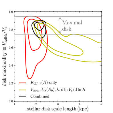
Figure 18 shows the joint PDF for the stellar disk scale length and the contribution of the stellar disk to the circular velocity at 2.2 scale lengths ( the peak of the disk rotation curve). The latter parameter determines whether the Milky Way’s disk is maximal using the definition of Sackett (1997), according to which a disk is maximal when its contribution to at 2.2 scale lengths is . We show the constraints from different combinations of the dynamical constraints. The red curves show the contours of the PDF based on the measurements from this paper only, while the black curves give the constraints based on all of the dynamical data. It is clear that the measurements of from this paper alone measure the scale length, largely independent of the contribution to the mass from the other Galactic components. Figure 18 also shows that the additional dynamical data from 5.1 does not constrain the stellar disk scale length. The joint PDF for the scale length and disk-maximality parameter based on the rotation curve and does show the familiar relation that for the disk to be maximal, the disk scale length needs to be small.
5.2.1 Constraints on the Galactic disk mass distribution
Therefore, we conclude that the measurements from this paper are the single most important existing dynamical constraint on the stellar disk scale length of the Milky Way. The result from the combined fit to all dynamical data gives
| (42) |
The combination of the measurements and the additional dynamical data shows that the disk is maximal since
| (43) |
These measurements of the stellar disk scale length and its contribution to the rotation curve allow us to derive the mass of the disk. We can measure the surface density of the stellar disk because the additional data on the rotation curve described in 5.1 combined with the measurements from this paper allow us to disentangle the stellar and dark-halo contributions to . We find that the surface density of the stellar disk at is , for a total surface density to of , of which is assumed to be in the thin ISM layer. As a consequence of ours being a full 3D dynamical model, this measurement of is a real measurement of as opposed to a measurement of converted to . The fact that it agrees so well with the local normalization of our measured profile in equation (27) is due to the fact that the local slope of the circular velocity curve is very close to flat in our best-fit model (see below). Our measurement of the local surface density to is consistent with all previous measurements (which are really measurements) but with a smaller uncertainty (Kuijken & Gilmore, 1989b; Siebert et al., 2003; Holmberg & Flynn, 2004; Bienaymé et al., 2006; Garbari et al., 2012; Zhang et al., 2013). We note in particular that the measurement of Garbari et al. (2012) of is consistent with our measurement; our much smaller errorbar leads to a much tighter measurement of the local dark matter density (see below).
As mentioned above, none of the dynamical data in 5.1 constrain the mass scale height of the stellar disk: we obtain a flat PDF for over the prior range . To illustrate how can be constrained using measurements of the (surface density) at heights different from , we fit the dynamical data from 5.1 together with the constraint on the total midplane density at from Holmberg & Flynn (2000): . While all of the other dynamical parameters are unchanged, in this case we do constrain the mass scale height: , in good agreement with the measurements from star counts (, see above and BO12d) and constraints from the vertical profile of ( at confidence; Zhang et al. 2013).
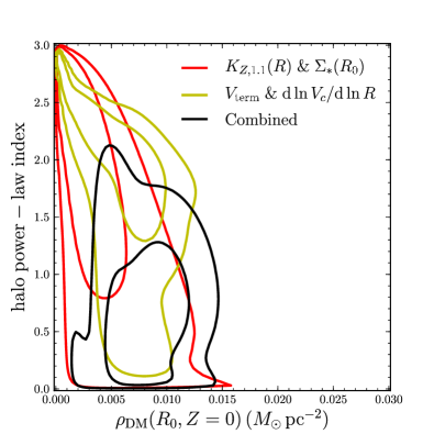
Using our measurements of the disk mass scale length and the local disk normalization, we can derive the total mass of the disk, to the extent that a characterization of the disk with a single scale length makes sense. We find that the total stellar disk mass is . Under our assumption that the local ISM column density is and that the ISM layer has a scale length twice that of the stellar disk, the ISM contributes for a total (stars+gas) disk mass of . Note that in our model the ISM layer’s scale length is tied to that of the stellar disk and that the local normalization is fixed. Therefore, the mass of the ISM layer is perfectly correlated with that of the stellar disk, and the uncertainty in the total disk mass would be . For this reason, we have added an uncertainty of , or almost of the ISM mass, in quadrature to the formal uncertainty in the disk mass. The bulge contributes another (Binney & Tremaine, 2008), while the stellar halo mass is negligible, such that the total baryonic mass of the Milky Way is
| (44) |
assuming an uncertainty of on the bulge mass. To derive these masses, we have assumed that . Changing to a different value does not change the measurements made in this subsection or in subsequent subsections, except for the total masses, which all increase by when increasing to ; this change is approximately linear in . The change is so large because of the short scale length of the disk: a small change in leads to a big change in . All other measurements are independent of , in particular the disk scale length, disk maximality at , and the local surface densities.
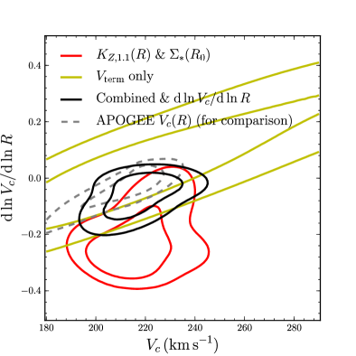
Our finding that the Milky Way’s disk has a short scale length raises the question of whether such a massive disk is stable to axisymmetric perturbations, i.e., whether Toomre’s (Toomre, 1964). We do not discuss this here in detail as this needs to be looked at carefully, accounting for the mix of different components of the disk and their radial dispersion profiles (which are poorly constrained currently), and for the finite thickness of the disk.
5.2.2 Constraints on the dark matter halo
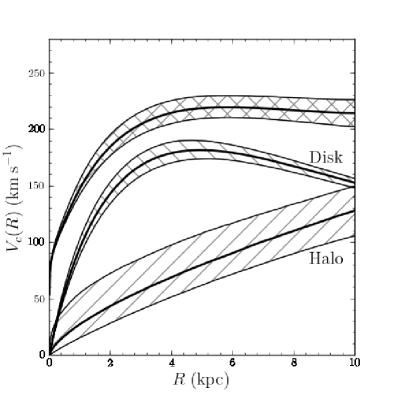
A plausible way toward measuring the local dark halo density profile is to combine the rotation curve, which measures the total mass as a function of radius but is relatively insensitive to the flattening and therefore cannot separate the disk’s contribution from the halo’s, with independent measurements of the disk contribution as a function of radius, as provided in this paper. The constraints on the halo parameters—the local normalization and power-law index in —from our data marginalized over all other mass-model parameters (including ) are shown in Figure 19. We show the constraints from measurements of the vertical dynamics ( and ) and those from the rotation curve (terminal velocities and ) alone; neither of these constrains the radial profile of the dark halo and the entire prior range is allowed at . However, the combination of these two dynamical probes allows us to put a first constraint on the radial profile. The combination gives
| (45) |
This encompasses a cored halo as well as an NFW halo, although very steep halo density profiles are ruled out. We constrain the local dark matter density to be , consistent with more direct measurements of this quantity (e.g., Bovy & Tremaine, 2012; Zhang et al., 2013), which measure the dark matter density using the vertical dependence of () rather than the radial dependence of as we do here.
5.2.3 Constraints on the rotation curve
Finally, while we do not measure the local circular velocity in a direct manner, we do constrain it indirectly in its guise of providing the normalization of the forces in our model and thus setting the mass scale. A comparison between the value of measured in this way and more direct measurements can therefore test whether the vertical dynamics is consistent with the planar dynamics. Figure 20 shows the joint PDF for the local and the local logarithmic slope of the rotation curve, . The constraints from the terminal velocities alone show the familiar degeneracy, indicating that the terminal velocities only measure a combination of and the slope of . The constraints from the vertical dynamics (red curves) have a different degeneracy and strongly disfavor rising rotation curves. The combination of the terminal velocities and the vertical dynamics therefore measures the properties of the circular velocity curve, and we find that and , consistent with a flat rotation curve. These measurements are consistent with the recent APOGEE measurements of Bovy et al. (2012a), which are shown for comparison. They are also consistent with the measurement of the angular rotation frequency at the Sun by Feast & Whitelock (1997) who found and . We emphasize that our measurement of in this paper does not rely on the Sun’s peculiar rotational velocity. For a further discussion of how a measurement of compares with the literature we refer the reader to Section 5.3 of Bovy et al. (2012a); suffice it to say that all previous measurements are consistent with this measurement. A combination of the data considered in this paper with the APOGEE results gives and . As the measurements of this paper and the APOGEE measurements are very different in the way that they probe the dynamics of the disk, the fact that these two measurements agree on strongly argues that .
Figure 21 shows a different representation of all of the results described in this Section. Shown are the total rotation curve and its decomposition into stellar-disk and halo contributions. The total and stellar-disk rotation curves are quite tightly constrained by our dynamical data. This is mostly due to our precise measurement of the stellar disk scale length, which was made possible by our measurements of over . The dark halo contributes significantly less to than the stellar-disk at all . Figure 21 decidedly shows that we have for the first time clearly—and through direct dynamical measurement—separated the disk and halo contributions to the Milky Way’s rotation curve.
6. Discussion
6.1. First dynamical measurement of the Milky Way’s scale length
We believe that this paper presents the first dynamical measurement of the Milky Way disk’s mass profile. Other measurements of the scale length are either based on star counts and it is therefore unclear whether they trace all of the mass in the disk (e.g., Jurić et al. 2008, BO12d), or they are based on previous dynamical data that leave the scale length essentially unconstrained (Dehnen & Binney 1998; Figure 18) unless strong priors are used (e.g., McMillan, 2011). It turns out that our best-fit model for the mass distribution in the inner of the Milky Way is similar to that of model I in Binney & Tremaine (2008), which has a maximal disk with a scale length of .
If star counts do trace the underlying mass distribution, then we can compare our dynamically-inferred scale length with that measured from star counts. There have been many measurements over the last few decades of the radial scale lengths of the thin and thick-disk components spanning a wide range between and . These measurements have greatly improved over the last few years with the advent of larger-area surveys with precise multi-band photometry leading to better photometric distances. For example, Gould et al. (1996) measured a scale length of from HST star counts of M dwarfs, whose distribution is expected to trace that of the underlying stellar mass, and Jurić et al. (2008) found from an analysis of SDSS star counts that the thin disk scale length is . Both of these are somewhat larger than the scale length measured in this paper. This offset may be due to systematic uncertainties in the photometric distances used by analyses of star counts. Another, in our view more likely explanation is that these analyses did not take into account that the radial scale lengths of different stellar disk components vary strongly. In particular, the scale lengths of the old, thick components of the disk are only (Bensby et al. 2011; BO12d; Cheng et al. 2012). This lowers the scale length of the mass profile compared with that of the thin-disk components, an effect which is larger at , where most of our measurements lie.
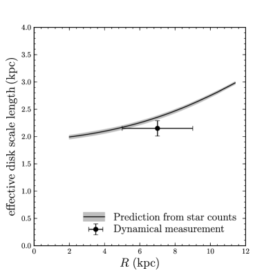
A proper comparison between the dynamically-inferred scale length and that measured from star counts should therefore take into account the full, complex structure of the disk. BO12 showed that the disk is made up of many components with scale lengths ranging from for the oldest populations to for the younger populations. The mass scale length of the stellar disk is determined by the sum of all of these components, whose combined density profile defines an effective disk scale length at every radius. This effective disk scale length based on the re-assembly of the MAP decomposition of BO12 is shown in Figure 22 (the MAP scale lengths of BO12d have been re-scaled to the An09 distance scale). The stellar mass profile derived from summing over all MAPs is not a single exponential, but has a profile whose effective disk scale length increases smoothly from in the inner disk to at . The dynamical measurement from this paper compares well with that inferred from star counts: the dynamical estimate falls short of the star-counts measurement by about . Nevertheless, this comparison lends credence to the interpretation that the stars in the Galactic disk are indeed the dominant contributors to the ‘dynamically inferred disk mass’ derived here. With measurements in the outer disk at , the MAP star-counts model predicts that one should dynamically measure a mass scale length .
We can further compare our dynamical measurement of the stellar-disk surface density at , , with estimates based on direct star counts. Estimates of the total amount of ordinary stellar matter are (Flynn et al. 2006;BO12b) with an additional contributed by stellar remnants and brown dwarfs (Flynn et al., 2006). These estimates have uncertainties of a few , which includes the uncertainty in the shape of the initial mass function at low masses (see BO12b). Thus, our dynamical measurement of the disk mass properties is in excellent agreement with direct star-counts.
That the dynamical and star-counts measurements of the stellar-disk scale length and of the local stellar surface density agree so well is evidence that basically all of the mass in the stellar disk is accounted for by ordinary stellar matter orbiting under the influence of Newtonian gravity. Our results leave little room for a dark disk component in the Milky Way (Read et al., 2008), because the presence of such a component would increase our estimates of the local surface density and of the mass scale length. Similarly, in the MOND theory of modified gravity the local surface-density to is predicted to be enhanced with respect to the contribution from baryonic matter by 444A simple way to see this is that the vertical force in MOND is enhanced by the same amount as the radial force. From Figure 21 it is clear that in Newtonian gravity the disk only provides about of the radial force at , such that MOND needs to enhance the radial, and consequentially the vertical, force by . (Nipoti et al., 2007; Bienaymé et al., 2009; Famaey & McGaugh, 2012), such that we expect for that . This prediction is in tension with our measurement of . Furthermore, in MOND the dynamically-inferred disk scale length (i.e., that inferred from measurements) is predicted to be larger than that measured from star counts (Bienaymé et al., 2009), so we would expect to dynamically measure a scale length of . This is removed from our measurement of the mass scale length. We emphasize that these are preliminary tests of MOND based on the Bekenstein–Milgrom (Bekenstein & Milgrom, 1984) formulation of MOND and that these tests should more fully take into account the uncertain structure of the baryonic disk. However, it is clear that the measurements from this paper and further improved measurements of the vertical forces in the Milky Way are key to improved tests of modified gravity models such as MOND on galaxy scales.
6.2. The mass of the Galactic disk
Our measurement of the mass scale length of the disk now makes our measurement of the Galactic disk mass the most accurate estimate to date. Our measurement of compares well with the range found by Flynn et al. (2006) (who also assume ), who estimated the stellar-disk mass as a function of an assumed scale length. Our measurement of the scale length falls at the lower end of their considered range where their stellar disk mass is . Our estimate of the baryonic mass in the Galaxy of also agrees with their estimate of . However, it is important to note that ours is a purely dynamical measurement, while Flynn’s value relies on assumptions about the stellar mass function in the disk and about the manner in which mass traces light. Both measurements are similarly affected by the uncertainty in .
6.3. Disk maximality and the Milky Way compared to external galaxies
The measurements of the Milky Way’s disk mass scale length and stellar mass from this paper allow us to make comparisons of the Milky Way with external galaxies, e.g., through the Tully-Fisher relation, initially put forth by Flynn et al. (2006), more precise. A main source of systematic uncertainty in Flynn et al. (2006) was the uncertainty in the value of the radial scale length, which a priori could have been anywhere between and . Our measurement of removes this source of uncertainty. Using Flynn et al. (2006)’s calculations of the total -band luminosity of the Milky Way we find that (). Using a bulge luminosity of (Kent et al., 1991), we find that
| (46) |
Combined with our measurement that , this allows us to place the Milky Way onto the Tully-Fisher relation defined by nearby disk galaxies: it falls well within the scatter (e.g., Dale et al., 1999) as this relation predicts for with a scatter of . Therefore, from the point of view of the Tully-Fisher relation, the Milky Way is a typical galaxy.
The decomposition of the Milky Way’s rotation curve into the contributions from the stellar disk and the dark-matter halo in 5.2 has shown that the Milky Way’s disk is maximal by the definition of Sackett (1997). This appears to be in conflict with arguments based on the lack of correlation between Tully-Fisher velocity residuals and disk size for external galaxies (Courteau & Rix, 1999), which have been used to argue against disks being maximal. However, whether this really shows that all disks are sub-maximal is far from clear, as dynamical modeling of gas kinematics in various galaxies and constraints from spiral structure have shown that some disks, especially those with , are maximal (Athanassoula et al., 1987; Weiner et al., 2001; Kranz et al., 2003), while being consistent with the considerations of Courteau & Rix (1999). Measurements of the vertical velocity dispersions of external galaxies have been interpreted to indicate that disks are substantially sub-maximal (e.g., Bottema 1997 and more recently Kregel et al. 2005 and Bershady et al. 2011). Such measurements rely on the same dynamical principles as those employed in this paper’s measurement, but these are much more difficult to apply in external galaxies without strong assumptions. It is essentially impossible to measure both the scale height and the vertical velocity dispersion for any individual external galaxy; further the velocity dispersions obtained from integrated light do not trace the older, dynamically-relaxed stellar populations very well. As such, these measurements are afflicted with systematic uncertainties, which have not been sufficiently investigated. The fact that the Milky Way would appear substantially sub-maximal in the analysis of Bershady et al. (2011) while the detailed dynamical modeling in this paper indicates otherwise may be a sign of these systematic uncertainties555A specific example is the following: Bershady et al. (2011) use the scale length of as a proxy for that of and use the latter as a proxy for the disk scale length. Neither of these are good proxies in the Milky Way: in BO12c we measured the scale length of to be , which is much longer than that of found in 4.2; in this paper we find that the scale length of is significantly longer than that of . As Bershady et al. (2011) use the scale length of to estimate galaxy disks’ central surface density , these effects lead one to underestimate and the maximality parameter of external disks..
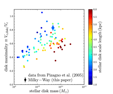
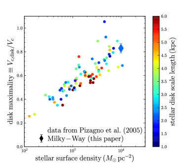
In Figure 23 we compare our measurements of the Milky Way disk’s properties to those derived from a sample of 81 disk-dominated galaxies from Pizagno et al. (2005). We follow Gnedin et al. (2007) in using the measurements of the disk scale lengths, stellar masses, and circular velocities at 2.2 disk scale lengths to derive the disk’s contribution to the rotation curve at 2.2 disk scale lengths. In detail, we scale the stellar masses down by 20% to correct them for the presence of any bulge component and we lower the observed scale lengths by 10% as these scale lengths are measured from and -band images, which are typically larger than the -band scale length, which better traces the stellar mass (de Jong, 1996). The top panel shows that the Milky Way falls nicely within the stellar-mass–disk-maximality relation derived from the Pizagno et al. (2005) data. However, the Milky Way’s scale length is quite different from that of external galaxies with similar stellar masses: for its stellar mass, the Milky Way would be expected to have scale length of , albeit it with a large scatter of ; this is clear from the color-coding of the points in the top panel of Figure 23. Following Gnedin et al. (2007), we also consider the relation between the disk’s surface density () and the fraction of the circular velocity contributed by the disk. This is shown in the bottom panel of Figure 23. The short scale length that we measure for the Milky Way has the effect of putting the Milky Way at the upper edge of the observed surface densities, but the Milky Way still falls along the general trend determined by external galaxies.
Therefore, if the Milky Way is atypical in any way, it is because of its short scale length. However, the mass-weighted scale length is only poorly measured for external galaxies, because variations in the mass-to-light ratio with radius may hamper the photometrically measured disk profiles.
6.4. MAPs as dynamically phase-mixed populations
The analysis in this paper has used the properties of MAPs as measured in BO12 to justify modeling the MAPs as phase-mixed, steady-state stellar populations that lend themselves to simple dynamical models. This has worked well and all MAPs lead to a consistent measurement of the vertical mass distribution near the disk. The single-qDF-per-MAP model provides a good fit to the spatial and kinematic properties of MAPs, as explicitly shown in the detailed comparisons between the data and the best-fit dynamical models in Appendix B. Thus, the MAPs are indeed well-described by the action-based qDF, as first proposed by Ting et al. (2013), although with the caveat that we have not modeled the radial and azimuthal velocities.
The fact that all MAPs can be described by the qDF adds further to the evidence that MAPs are simple dynamical building blocks of the (local) disk, as first proposed by BO12. In particular the MAPs with scale heights and velocity dispersions intermediate between those of the canonical thin and thick disk are real dynamical populations. If these intermediate MAPs would have arisen because of abundance errors, as was already strongly argued against based on their observed spatial properties and kinematics in BO12, we would not expect to be able to model them using a consistent dynamical model. For example, we would expect that the vertical profile measurements would be dominated by the stars in the thin component, while the dispersion measurements would be dominated by the stars in the thicker, kinematically-warmer component, which would strongly overestimate the surface density (by a factor of 3 or more). The fact that this does not happen strongly argues that the intermediate MAPs are real, phase-mixed stellar populations in a dynamical steady state.
7. Conclusions
In this paper we have used six-dimensional dynamical fitting employing three-action-based distribution functions, in order to model abundance-selected stellar populations from the SEGUE survey, fully accounting for the selection function and deriving dynamical constraints while marginalizing over properties of the DF. We have used this in particular to obtain a measurement of (or ) at a single Galactocentric radius for each MAP, thus dynamically measuring for the first time the radial profile of the surface density near the disk. These measurements are given in Table 6 and they present stringent new constraints on the mass distribution in the inner Milky Way.
We have used these new measurements of in addition to (weak) existing measurements of the terminal velocity curve between and , the contribution of the disk to the local surface density, and the local slope of the rotation curve to constrain the gravitational potential between and . We find that our new measurements of provide the only dynamical constraint able to measure the dynamical (mass-weighted) disk scale length; in combination with the other dynamical constraints we can measure the properties of the Milky Way’s disk to great precision and find
where includes the contributions from ordinary stellar matter, stellar remnants, and brown dwarfs and . We further find that
The systematic uncertainty is due to the uncertainty in : increasing from our fiducial value of to increases the estimated masses by . The disk mass includes the mass of the stellar disk, , as well as the mass of the ISM layer; is the total baryonic mass of the Milky Way, including the stellar and ISM disks and the bulge.
These direct dynamical measurements of the stellar disk’s properties are in good agreement with measurements derived from star counts, leaving little room for dark matter in a disk-like configuration. With a scale length this short, the Milky Way’s disk is maximal by the definition of Sackett (1997): we find that at 2.2 disk scale lengths.
This paper’s measurement of the disk mass will also be particularly valuable when measuring the dark halo’s flattening from constraints on the potential at larger heights. For example, Koposov et al. (2010) measured the total potential flattening at from the plane from fitting an orbit to the cold GD-1 stream, but found that the uncertainty in the mass of the disk did not allow for this to be turned into an interesting constraint on the halo’s flattening. Using our measurement of the disk mass, the GD-1 data indicate that the halo density flattening is , but it is clear that a more rigorous combination of these measurements and further progress in the dynamical fitting of tidal streams (e.g., Sanders & Binney, 2013) are necessary to robustly measure the halo’s flattening.
These measurements of the disk’s properties allow us to separate the contribution from the disk and the halo to the rotation curve, as shown in Figure 21. The halo does not contribute much to the Milky Way’s rotation curve at . In turn this means that our constraints on the radial profile of the dark halo are relatively weak. Nevertheless, these are the first dynamical constraints on the radial distribution of dark matter at and we find for a model that at 95 % confidence (where indicates that our measurement is based on dynamical data at ). Further measurements of the vertical mass distribution (e.g., at and ) would significantly improve this constraint.
The dynamical modeling performed in this paper is complex, computationally expensive, and currently limited to exploring only a few parameters of the gravitational potential. It provides a full generative modeling framework in which selection effects, observational uncertainties, nuisance parameters, outlier models, and other data issues can be naturally included using a likelihood-based approach. We have dealt with the computational complexity by focusing our efforts on the measurement of a single dynamical constraint derived from each dynamical sub-sample of stellar tracers (MAPs): the vertical force at . However, it is clear that the fitting procedure to each MAP can yield much more information than this. In particular, each sub-sample could be used to also measure the vertical profile of the vertical force within the SEGUE sample’s spatial volume, which should lead to better constraints on the radial profile of the dark-matter halo. Ultimately, this is what is required for the optimal analysis of Gaia data. The analysis in this paper has demonstrated 3D, 3-action dynamical modeling of disk populations using observations of individual stars in the context of a real data set with all of the complexities of a non-trivial selection function and data uncertainties. But it is clear that further development of this technique, especially in more efficiently exploring the dynamical PDF, is necessary before the Gaia data arrive.
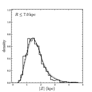
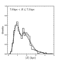
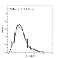
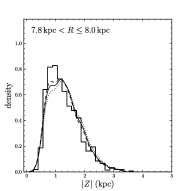
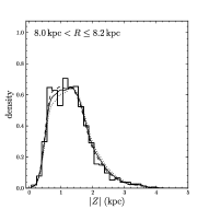
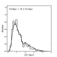
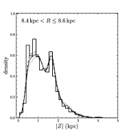
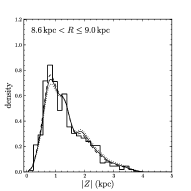
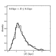
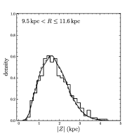
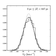
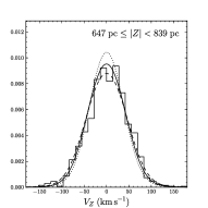
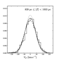
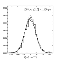
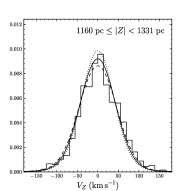
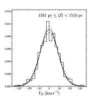
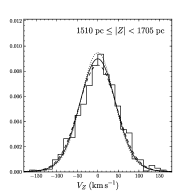


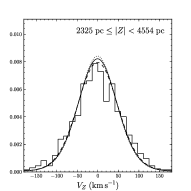
Appendix A Calculation of the effective survey volume
In this Appendix we describe how we can efficiently calculate the 8-dimensional normalization integral (the effective survey volume) in the likelihood in equation (25). This calculation is similar to that in the case of the density fits in BO12d as described in their Appendix B, and we start from their equation (B4), re-written to include the velocity integration
| (A1) |
where
| (A2) |
is the spatial density predicted by the DF.
To evaluate the expression in equation (A1) efficiently, we split the calculation in two steps: (1) We calculate the predicted spatial density in equation (A2) on a grid in and interpolate it; (2) we use the interpolated density to evaluate the sums in equation (A1). We perform the velocity integration in equation (A2) by using 20-th order Gauss-Legendre integration in each direction: from 0 to for the tangential velocity and from to for the radial and vertical velocity. ‘’ is calculated using the scale dispersion profiles of the DF (see equations [3-5])). We calculate the density on a grid of points ranging from 4 to in and from to in and interpolate using 3-th order two-dimensional spline interpolation.
Appendix B Detailed data versus model comparisons
In this Appendix we describe the results from detailed comparisons between the best-fit dynamical models for individual MAPs obtained using the methodology described in 3 and the SEGUE data. As in BO12d, we do this in a space close to that of the raw data: star counts uncorrected for selection effects. Even though our model is a full generative model that could predict the distribution of any combination of to be compared with the data, because we are mainly concerned with measuring , we focus here on (a) vertical number counts and (b) the distribution of vertical velocities, both as a function of radius, as these are the main data ingredients for constraining . As described in 3, we fit individual MAPs that typically only have a few hundred stars, making visual comparisons between the data and the model highly susceptible to the influence of Poisson noise. For this reason and because showing comparisons for 43 different sub-samples would take up the better part of an ApJ volume, we group MAPs into three main divisions with similar DFs. These are (a) -old MAPs, i.e., all MAPs with ; these MAPs all have short radial scale lengths around , and they are vertically thick. (b) -young MAPs, i.e., those with ; these are vertically thin and have longer scale lengths. Finally, we consider MAPs intermediate between (a) and (b), which are all of the MAPs with and . We calculate the predicted number counts for each MAP within a sub-division separately and plot the sum of all predictions, weighted by relative number of data points in different MAPs.
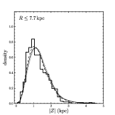
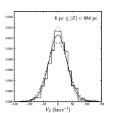

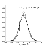
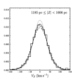
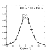
The sub-division of -old MAPs is by far the largest of the three sub-divisions, allowing us to closely investigate the goodness of the dynamical fit as a function of . Figure 24 shows the comparison between the predicted number counts as a function of distance from the plane and the data, in 10 different radial bins that each contain about stars. The number counts for these -old populations are reproduced excellently by our dynamical model to almost every single wiggle. As -old MAPs primarily measure at (see Figure 12), we also include the predictions from models with very different from the best-fit model. All three models shown predict almost the same number-counts profile.
The distribution of vertical velocities as a function of position for 10 different bins in distance from the midplane is shown in Figure 25. These distributions show excellent agreement between the data and the best-fit model over the full range of distances from the plane, from to . The alternative models slightly overestimate or underestimate the width of the distribution, depending on whether their disk is too heavy or too light. From Figures 24 and 25 it is clear that the number-count measurements are the most informative, such that the dynamical fit works essentially as follows: (a) for a given potential, the qDF parameters are adjusted to match the observed number counts without regard as to whether the vertical velocities are fit well; (b) the best-fitting potential is the one for which these qDF parameters also fit the vertical velocity distribution. This is essentially the same procedure that was used more explicitly by Kuijken & Gilmore (1989a).
Figure s 26 and 27 show similar comparisons for the intermediate MAPs. These demonstrate that the vertical number counts are matched well, although with a slight overprediction of the scale height around . Heavier and lighter disks (with changes to around for intermediate MAPs) again predict almost the same vertical profile. Figure 27 shows that the distribution of vertical velocities as a function of height is excellently fit by the best-fit dynamical model; the predictions of the heavier and lighter disks are obviously ruled out for these populations.
Finally, Figure s 28 and 29 show data–model comparisons for the -young populations, split only into two radial and vertical bins here because only about stars have in our selection of the SEGUE G-type dwarfs. The comparison is therefore not as fine-grained as for the -old and intermediate divisions, but the correspondence between the data and the model are similar as for the other divisions: the vertical number-count profiles are predicted to be similar for the best-fit potential and the heavier- and lighter-disk alternative models; the distribution of the vertical velocities clearly prefers the best-fit model over the alternatives.
The fact that both the vertical number counts and the distribution of vertical velocities is matched in detail by our 3-action based qDF model proves that a description of these populations as dynamically-relaxed populations makes sense. However, the detailed comparison of the vertical number-counts of the best-fit dynamical model and the data for all three sub-divisions shows a slight underprediction of the number counts at and , which is likely due to substructure that is not captured by our model. Clearly, investigation of the residuals from the best-fit dynamical models for MAPs in the future will be useful for determining the fine-grained orbital structure of MAPs, which may contain traces of dynamical or accreted substructures.
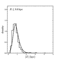
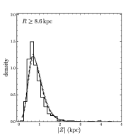
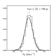
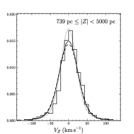
References
- Allende Prieto et al. (2008) Allende Prieto, C., Sivarani, T., Beers, T. C., et al. 2008, AJ, 136, 2070
- An et al. (2009) An, D., Pinsonneault, M. H., Masseron, T., et al. 2009, ApJ, 700, 523 (An09)
- Athanassoula et al. (1987) Athanassoula, E., Bosma, A., & Papaioannou, S. 1987, A&A, 179, 23
- Bekenstein & Milgrom (1984) Bekenstein, J. & Milgrom, M. 1984, ApJ, 286, 7
- Bell & de Jong (2001) Bell, E. F. & de Jong, R. S. 2001, ApJ, 550, 212
- Bell et al. (2003) Bell, E. F., McIntosh, D. H., Katz, N. & Weinberg, M. D. 2003, ApJS, 149, 289
- Bensby et al. (2011) Bensby, T., Alves-Brito, A., Oey, M. S., Yong, D., & Meléndez, J. 2011, ApJ, 735, L46
- Bershady et al. (2011) Bershady, M. A., Martinsson, T. P. K., Verheijen, M. A. W., Westfall, K. B., Andersen, D. R., & Swaters, R. A. 2011, ApJ, 739, L47
- Bienaymé et al. (2006) Bienaymé, O., Soubiran, C., Mishenina, T. V., Kovtyukh, V. V., & Siebert, A. 2006, A&A, 446, 933
- Bienaymé et al. (2009) Bienaymé, O., Famaey, B., Wu, X., Zhao, H. S., & Aubert, D. 2009, A&A, 500, 801
- Binney & Evans (2001) Binney, J. J. & Evans, N. W. 2001, MNRAS, 327, 27
- Binney & Tremaine (2008) Binney, J. & Tremaine, S. 2008, Galactic Dynamics: Second Edition
- Binney (2010) Binney, J. J. 2010, MNRAS, 401, 2318
- Binney & McMillan (2011) Binney, J. J. & McMillan, P. 2011, MNRAS, 413, 1889
- Binney (2012a) Binney, J. J. 2012a, MNRAS, 426, 1324
- Binney (2012b) Binney, J. J. 2012b, MNRAS, 426, 1328 (Princeton University Press)
- Bottema (1997) Bottema R. 1997, A&A, 328, 517
- Bovy et al. (2009) Bovy, J., Hogg, D. W., & Rix, H.-W. 2009, ApJ, 704, 1704
- Bovy et al. (2012a) Bovy, J., Allende Prieto, C., Beers, T. C., et al. 2012a, ApJ, 759, 131
- Bovy et al. (2012b) Bovy, J., Rix, H.-W., & Hogg, D. W. 2012b, ApJ, 751, 131 (BO12b)
- Bovy et al. (2012c) Bovy, J., Rix, H.-W., Hogg, D. W., et al. 2012c, ApJ, 755, 115 (BO12c)
- Bovy et al. (2012d) Bovy, J., Rix, H.-W., Liu, C., et al. 2012d, ApJ, 753, 148 (BO12d)
- Bovy & Tremaine (2012) Bovy, J., & Tremaine, S. 2012, ApJ, 756, 89
- Brent (1973) Brent, R. P. 1973, Algorithms for Minimization Without Derivatives (Prentice-Hall: Englewood Cliffs, NJ)
- Chen et al. (2001) Chen, B., Stoughton, C., Smith, J. A., et al. 2001, ApJ, 553, 184
- Cheng et al. (2012) Cheng, J., Rockosi, C. M., Morrison, H. L., et al. 2012, ApJ, 752, 51
- Clemens (1985) Clemens, D. P. 1985, ApJ, 295, 422
- Courteau & Rix (1999) Courteau, S. & Rix, H.-W. 1999, ApJ, 513, 561
- Dale et al. (1999) Dale, D. A., Giovanelli, R., Haynes, M. P., Campusano, L. E., & Hardy, E. 1999, AJ, 118, 1489
- Dehnen & Binney (1998) Dehnen, W. & Binney, J. 1998, MNRAS, 294, 429
- de Jong (1996) de Jong, R. S. 1996, A&A, 313, 377
- Famaey & McGaugh (2012) Famaey, B. & McGaugh, S. S. 2012, Living Reviews in Relativity, 15, 10
- Feast & Whitelock (1997) Feast, M. & Whitelock, P. 1998, MNRAS, 291, 683
- Flynn et al. (2006) Flynn, C., Holmberg, J., Portinari, L., Fuchs, B., & Jahreiß, H. 2006, MNRAS, 372, 1149
- Garbari et al. (2012) Garbari, S., Liu, C., Read, J. I., & Lake, G. 2012, MNRAS, 425, 1445
- Ghez et al. (2008) Ghez, A. M., Salim, S., Weinberg, N. N., et al. 2008, ApJ, 689, 1044
- Gillessen et al. (2009) Gillessen, S., Eisenhauer, F., Trippe, S., Alexander, T., Genzel, R., Martins, F., & Ott, T. 2009, ApJ, 692, 1075
- Gnedin et al. (2007) Gnedin, O. Y., Weinberg, D. H., Pizagno, J., Prada, F., & Rix, H.-W. 2007, ApJ, 671, 1115
- Gould et al. (1996) Gould, A., Bahcall, J. N., & Flynn, C. 1996, ApJ, 465, 759
- Holmberg & Flynn (2000) Holmberg, J. & Flynn, C. 2000, MNRAS,313, 209
- Holmberg & Flynn (2004) Holmberg, J. & Flynn, C. 2004, MNRAS,352, 440
- Ivezić et al. (2008) Ivezić, Ž., Sesar, B.; Jurić, M., et al. 2008, ApJ, 684, 287 (I08)
- Jurić et al. (2008) Jurić, M., Ivezić, Ž., Brooks, A., et al. 2008, ApJ, 673, 864
- Kent et al. (1991) Kent, S., Dame, T. M., & Fazio, G. 1991, ApJ, 378, 131
- Koposov et al. (2010) Koposov, S. E., Rix, H.-W., & Hogg, D. W. 2010, ApJ, 712, 260
- Kranz et al. (2003) Kranz, T., Adrianne Slyz, A., & Rix, H.-W. 2003, ApJ, 586, 143
- Kregel et al. (2005) Kregel, M., van der Kruit, P. C., & Freeman, K. C. 2005, MNRAS, 358, 503
- Kuijken & Gilmore (1989a) Kuijken, K. & Gilmore, G. 1989a, MNRAS, 239, 571
- Kuijken & Gilmore (1989b) Kuijken, K. & Gilmore, G. 1989b, MNRAS, 239, 605
- Lee et al. (2011a) Lee, Y. S., Beers, T. C., Allende Prieto, C., et al. 2011a, AJ, 141, 90
- Lee et al. (2011b) Lee, Y. S., Beers, T. C, An, D., et al. 2011b, ApJ, 738, 187
- Lee et al. (2008a) Lee, Y. S., Beers, T. C., Sivarani, T., et al. 2008a, AJ, 136, 2022
- Lee et al. (2008b) Lee, Y. S., Beers, T. C., Sivarani, T., et al. 2008b, AJ, 136, 2050
- Lewis & Freeman (1989) Lewis, J. R. & Freeman, K. C. 1989, AJ, 97, 139
- Li & White (2009) Li, C. & White, S. D. M. 2009, MNRAS, 398, 2177
- Margorrian (2006) Magorrian, J. 2006, MNRAS, 373, 425
- McClure-Griffiths & Dickey (2007) McClure-Griffiths, N. M. & Dickey, J. M. 2007, ApJ, 671, 427
- McMillan (2011) McMillan, P. 2011, MNRAS, 414, 2446
- McMillan & Binney (2012) McMillan, P. & Binney, J. J. 2012, MNRAS, 419, 2251
- McMillan & Binney (2013) McMillan, P. & Binney, J. J. 2013, MNRAS, 433, 1411
- Munn et al. (2004) Munn, J. A., Monet, D. G., Levine, S. E., et al. 2004, AJ, 127, 3034
- Navarro et al. (1997) Navarro, J. F., Frenk, C. S., & White, S. D. M. 1997, ApJ, 490, 493
- Nipoti et al. (2007) Nipoti, C., Londrillo, P., Zhao, H. S., & Ciotti, L. 2007, MNRAS, 379, 597
- Pizagno et al. (2005) Pizagno, J., Prada, F., Weinberg, D. H., Rix, H.-W., Harbeck, D., Grebel, E. K., Bell, E. F., Brinkmann, J., Holtzman, J., & West, A. 2005, ApJ, 633, 844
- Popowski et al. (2005) Popowski, P., Griest, K., Thomas, C. L., et al. 2005, ApJ, 631, 879
- Read et al. (2008) Read, J. I., Lake, G., Agertz, O., & Debattista, Victor P. 2008, MNRAS, 389, 1041
- Reid et al. (2009) Reid, M. J., Menten, K. M., Zheng, X. W., et al. 2009, ApJ, 700, 137
- Rix & Bovy (2013) Rix, H.-W. & Bovy, J. 2013, A&A Rev., 21, 61
- Sackett (1997) Sackett, P. 1997, ApJ, 483, 103
- Sanders (2012) Sanders, J. 2012, MNRAS, 426, 128
- Sanders & Binney (2013) Sanders, J. L. & Binney, J. 2013, MNRAS, 433, 1826
- Schlesinger et al. (2010) Schlesinger, K. J., Johnson, J. A., Rockosi, C. M., et al. 2010, ApJ, 719, 996
- Schlesinger et al. (2012) Schlesinger, K. J., Johnson, J. A., Rockosi, C. M., et al. 2012, ApJ, 761, 160
- Schönrich et al. (2010) Schönrich, R., Binney, J. J., & Dehnen, W. 2010, MNRAS, 403, 1829
- Schönrich et al. (2012) Schönrich, R., Binney, J. J., & Asplund, M. 2012, MNRAS, 420, 1281
- Siebert et al. (2003) Siebert, A., Bienaymé, O., & Soubiran, C. 2003, A&A, 399, 531
- Siebert et al. (2008) Siebert, A., Bienaymé, O., Binney, J., et al. 2008, MNRAS, 391, 793
- Smolinski et al. (2011) Smolinski, J. P., Lee, Y. S., Beers, T. C., et al. 2011, AJ, 141, 89
- Ting et al. (2013) Ting, Y.-S., Rix, H.-W., Bovy, J., & van de Ven, G. 2013, MNRAS, 434, 652
- Toomre (1964) Toomre, A. 1964, ApJ, 139, 1217
- van Albada & Sancisi (1986) van Albada, T. S. & Sancisi, R. 1986, Philos. Trans. R. Soc. London, A, 320, 447
- Weiner et al. (2001) Weiner, B. J., Sellwood, J. A., & Williams, T. B. 2001, ApJ, 546, 931
- Yanny et al. (2009) Yanny, B., Rockosi, C., Newberg, H. J., et al. 2009, AJ, 137, 4377
- Zhang et al. (2013) Zhang, L., Rix, H.-W., van de Ven, G, Bovy, J., Liu, C., & Zhao, G. 2013, ApJ, 772, 108