Neutron Star Masses and Radii from Quiescent Low-Mass X-ray Binaries
Abstract
We perform a systematic analysis of neutron star radius constraints from five quiescent low-mass X-ray binaries and examine how they depend on measurements of their distances and amounts of intervening absorbing material, as well as their assumed atmospheric compositions. We construct and calibrate to published results a semi-analytic model of the neutron star atmosphere which approximates these effects for the predicted masses and radii. Starting from mass and radius probability distributions established from hydrogen-atmosphere spectral fits of quiescent sources, we apply this model to compute alternate sets of probability distributions. We perform Bayesian analyses to estimate neutron star mass-radius curves and equation of state (EOS) parameters that best-fit each set of distributions, assuming the existence of a known low-density neutron star crustal EOS, a simple model for the high-density EOS, causality, and the observation that the neutron star maximum mass exceeds . We compute the posterior probabilities for each set of distance measurements and assumptions about absorption and composition. We find that, within the context of our assumptions and our parameterized EOS models, some absorption models are disfavored. We find that neutron stars composed of hadrons are favored relative to those with exotic matter with strong phase transitions. In addition, models in which all five stars have hydrogen atmospheres are found to be weakly disfavored. Our most likely models predict neutron star radii that are consistent with current experimental results concerning the nature of the nucleon-nucleon interaction near the nuclear saturation density.
1 INTRODUCTION
Although the masses of at least 3 dozen neutron stars have been relatively precisely measured (see Lattimer (2012) for a summary), estimates of individual neutron star radii are poorly known. Additionally, simultaneous mass and radius measurements for the same object are relatively uncertain. The two leading candidates for such measurements are bursting neutron stars that show photospheric radius expansion (hereafter PRE; Van Paradijs 1979; Lewin, van Paradijs & Taam 1993) and transiently accreting neutron stars in quiescence (Rutledge et al., 1999), often referred to as quiescent low-mass X-ray binaries (QLMXBs). The former class of sources are believed to be energetic enough to temporarily lift the neutron star atmosphere off the surface and thus have peak luminosities near the Eddington Limit, where is the neutron star mass and is the atmospheric opacity. The luminosity on the tail of the burst, on the other hand, is due to thermal radiation from the cooling star, , where is the neutron star radius, is the effective blackbody temperature, and is a color-correction factor representing the fact that the atmosphere is not a true blackbody. Observations measure fluxes, so measurements of the luminosities require knowledge of the source distances . In addition, both the Eddington Limit and the observed luminosities must be corrected for gravitational redshift. These sources thus have the potential to measure two combinations of mass and radius.
The currently accepted theoretical explanation for the thermal X-ray emission from many QLMXBs is thermal energy deposited in the deep crust during outbursts (Brown, Bildsten & Rutledge, 1998). QLMXBs also exhibit hard nonthermal components (e.g., Campana et al. 1998), and the role played by low-level accretion is not well-understood (e.g., Rutledge et al. 2002a; Fridriksson et al. 2010). We ignore these potential complications in the current work and assume that this thermal energy further diffuses into and heats the core. Following outbursts, the energy is re-radiated on core-cooling timescales through the neutron star’s atmosphere. Since accretion of heavier elements leads to their gravitational settling on timescales of seconds (Romani, 1987; Bildsten, Salpeter & Wasserman, 1992), the atmosphere is usually assumed to be pure hydrogen. Pure H atmosphere models (Rajagopal & Romani, 1996; Zavlin, Pavlov & Shibanov, 1996; McClintock, Narayan & Rybicki, 2004; Heinke et al., 2006; Haakonsen et al., 2012) applied to QLMXBs often predict neutron star radii compatible with theoretical radius estimates, compared, for example, to blackbody models which would suggest km (Rutledge et al., 1999). Atmospheres dominated by heavier elements could occur when no hydrogen is accreted, such as is the case in some ultracompact X-ray binary systems like 4U 182030 where the donor is a helium white dwarf (Stella, Priedhorsky & White, 1987; Rappaport, et al., 1987). Recent work on helium atmospheres by (Servillat et al., 2012) and Catuneanu et al. (2013) based on models from Ho and Heinke (2009) have begun to clarify how they impact radius constraints in QLMXBs. QLMXBs are observed both in our Galaxy and in globular clusters, but distance uncertainties (of order 50%) associated with field sources precludes using them for accurate radius estimates. As opposed to PRE sources, QLMXBs primarily allow one to measure the angular diameter , where and, to much lesser accuracy through its weaker dependence on observed spectra, the gravitational redshift . Below, we always use to refer to the physical radius, not the radiation radius, which will always be written as .
Both types of measurements have large systematic errors, including their distances, the amount of interstellar absorption, and their atmospheric compositions. In addition, PRE burst sources have been largely modeled (Özel, Güver & Psaltis, 2009; Güver et al., 2010a, b; Özel, Baym & Güver, 2010; Steiner, Lattimer & Brown, 2010; Özel, Gould & Güver, 2012; Suleimanov, Poutanen & Werner, 2011; Steiner, Lattimer & Brown, 2013; Güver & Özel, 2013) with static, spherically symmetric atmospheres although they are certainly non-spherical, dynamical events. Another advantage of QLMXBs is that their atmospheric composition is likely to be pure H (or He, in the case of ultra-compact binaries) due to the rapid gravitational settling time of heavier elements in their atmospheres, while PRE atmospheres could be dominantly H or He and also have metallicities up to solar proportions.
A recent study of five QLMXBs by Guillot et al. (2013), hereafter G13, found that the best-fit physical radii of these five sources ranged from 6.6 km to 19.6 km if modeled with H atmospheres (see Table 4 in G13). Under the assumption that all the neutron stars have hydrogen atmospheres and the same radius, G13 determined this radius to be km to 90% confidence. Given the importance of well-measured neutron star radii for both astrophysics and nuclear physics (Lattimer & Prakash, 2001; Steiner & Gandolfi, 2012), we reconsider these five QLMXBs in the present study.
2 DATA AND FITS FOR QLMXBs
In this study, we will focus on the five QLMXB sources studied by G13, namely, the sources in M28, NGC 6397, M13, Cen, and NGC 6304. The X-ray spectra of at least two other sources, X7 in 47 Tuc (Heinke et al., 2006) and NGC 6553 (Guillot et al., 2011b), have been previously studied to generate mass and radius constraints. However, observations of the neutron star X7 in 47 Tuc are affected by pileup and those of the neutron star in NGC 6553 are contaminated from a nearby source (see discussion in G13). S. Guillot kindly provided us the probability distributions from the G13 spectral fits (these distributions did not include the distance uncertainty and did not assume that all neutron stars have the same radius).
| Source | (km) | Ref. | (km) | |||
|---|---|---|---|---|---|---|
| M28 | (1) | (G13) | ||||
| (2) | 1.89 (D90) | |||||
| 2.74 (H10) | ||||||
| NGC 6397 | 1.4 | (3) | (G13) | |||
| 1.4 (D90) | ||||||
| 1.23 (H10) | ||||||
| M13 | 0.11 | (4) | (G13) | |||
| 0.11 | (5) | 0.145 (D90) | ||||
| 0.12 | (6) | 0.137 (H10) | ||||
| Cen | 0.9 | (7) | (G13) | |||
| NGC 5139 | (8) | 1.04 (D90) | ||||
| 1.2 | (6) | 0.823 (H10) | ||||
| NGC 6304 | 2.66 | (9) | (G13) | |||
| 2.66 (D90) | ||||||
| 3.70 (H10) |
Note. — and values in columns 2 and 3 are those quoted by the references cited in column 4: (1) – Servillat et al. (2012); (2) – Becker et al. (2003); (3) – Guillot, Rutledge & Brown (2011a); (4) – Gendre, Barret & Webb (2003b); (5) – Catuneanu et al. (2013); (6) – Webb & Barret (2007); (7) – Rutledge et al. (2002b); (8) – Gendre, Barret & Webb (2003a); (9) – Guillot et al. (2009). The first row of columns 5, 6, and 7 for each source contains , , and values from G13 but recomputed to include distance uncertainties to excluding regions forbidden by the combination of causality and the minimum maximum mass constraints. In the second row, is set to Chandra Toolkit http://cxc.harvard.edu/toolkit/colden.jsp values (labelled D90). The third row has values using the reddening measurements from Harris (2010) with the correlation between and as discussed in Predehl & Schmitt (1995) and updated in Güver & Ozel (2009) (labelled H10). For the second and third rows, values are scaled according to Table 4 ( is unchanged by this procedure), and and are further corrected to account for causality and the minimum maximum mass constraints. All uncertainties reflect 90% confidence.
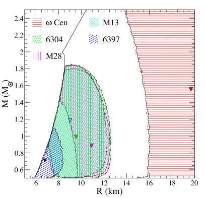
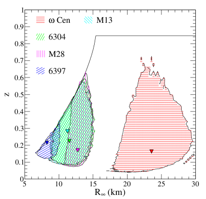
We use the distances and uncertainties given in G13 and presented in the second column of Table 1, and also assume their probability distributions can be modeled by Gaussians. Three of the globular clusters, NGC 6397, M13 and Cen, have dynamically-measured distances. M28 and NGC 6304 lack dynamical distance estimates. However, other distance measurements exist. The distance to NGC 6397 has been given as kpc in Gratton, et al. (2003) and kpc in Hansen et al. (2007). We adopt kpc as an alternate distance to the neutron star in NGC 6397. Also, Webb & Barret (2007) and Catuneanu et al. (2013) use kpc as the distance to M13 , which we also adopt as an alternative distance. These alternatives are given in the third column of Table 1. Together with the values from the second column for the other three sources, this set will be referred to as “Alt”.
It is worth pointing out that the Gratton, et al. (2003) and Hansen et al. (2007) distances for NGC 6397, which agree with a determination of 2.3 kpc from Harris (2010), are 28% larger than what G13 used and differ by much more than their quoted errors. Also, G13’s distance to M13 is 18% larger than those employed by Webb & Barret (2007) and Catuneanu et al. (2013). These differences have an impact on our results. Thus, there is a strong argument to also employ a set of distance estimates obtained with similar systematics. Among the largest analysis of globular cluster distances conducted in a fairly homogeneous fashion is that of Harris (2010). We arbitrarily choose to combine these with the uncertainties from G13 and refer to this set as H10 which appears in column four of Table 1. Because the inferred and coordinates of the distributions scale linearly with , is unaffected by the distance scale. In the work below, we rescale and resample the and coordinates of the distributions of G13 to obtain additional probability distributions and then translate these to distributions.
Previous works have also made different assumptions about the extent of X-ray absorption between the source and the observer. It has become commonplace to characterize the magnitude of the X-ray absorption by a single parameter, the “equivalent hydrogen column density” (we denote the column density in units of atoms cm-2 as ), which is the column density of atomic hydrogen which would most closely replicate the net obscuration of the spectrum including the effects of heavy elements in the intervening material. G13 determined together with the neutron star properties from spectral modeling, but the inferred values do not always agree with the value from HI maps summarized by Dickey & Lockman (1990). For each source, the first row in column 5 in Table 2 gives the G13 determination, while the second row contains values of according to the Chandra Proposal Planning Toolkit http://cxc.harvard.edu/toolkit/colden.jsp, hereafter referred to as CPPT. The CPPT lists Dickey & Lockman (1990) as its primary source, so we refer to these alternative equivalent hydrogen column densities as D90. We note that the values for for M28, M13 and Cen from the CPPT slightly differ from those G13 attributed to Dickey & Lockman (1990) (G13 gives 2.4, 0.11 and 0.9, respectively, for these sources). There are differences of up to 10-15% among the values given from HEARSAC [http://heasarc.gsfc.nasa.gov/docs/tools.html], CPPT, and the two HI surveys, Dickey & Lockman (1990) and Kalberla et al. (2005). We do not attempt to completely resolve these differences but choose a range of different values to systematically characterize the associated uncertainty.
Independent HI surveys are not necessarily good estimators of the true X-ray absorption. They can be overestimates near the plane of the galaxy where they include absorption from regions beyond the cluster. They do not include molecular H2, ionized H, and heavier elements, all of which can contribute to the absorption. Finally, the surveys do not always have sufficient spatial resolution to resolve the true column in the direction of the QLMXB and cannot account for absorption intrinsic to the globular cluster. To circumvent these problems, an approach often used is to take the HI surveys as a first guess, and improve that guess where possible using either reddening measurements or direct measurements of extinction from spectral fitting. As with the distance measurements, it is therefore useful to compare with results using uniform systematics, so we employ reddening measurements (Harris, 2010) together with the correlation between and X-ray-measured as discussed in Predehl & Schmitt (1995) and updated in Güver & Ozel (2009). These values are referred to as H10 in Table 2. It is interesting that the H10 values for are closer to the G13 values than are the D90 values for all the sources except for Cen.
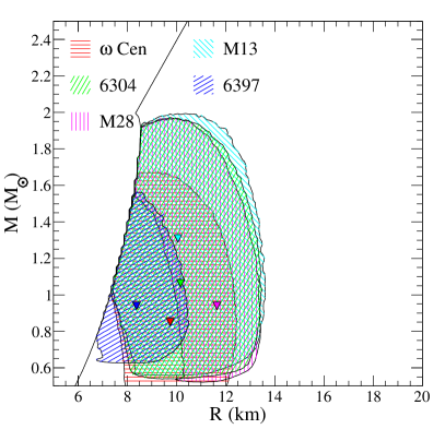
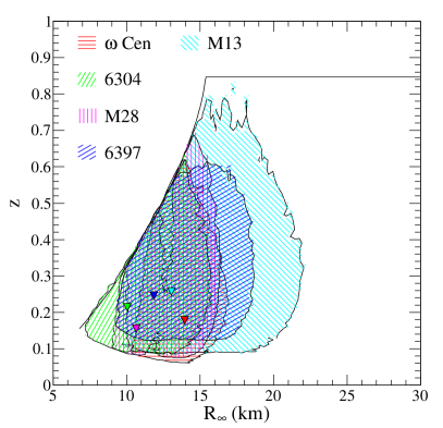
The probability distributions in space, which can be inferred from the results for the individual fits to each source in G13, tend to be banana-shaped, with the long axes approximately characterized by a fixed value of . It is therefore useful to use distributions rather than distributions. The 90% confidence intervals for the fits of G13 of , , and are shown in Fig. 1. An apparent feature of Fig. 1 is that the most-probable values of and span wide ranges so that and for the 5 sources do not appear to follow traditional curves for baryonic stars. In fact, it seems that and are roughly linearly related. This implies these sources have similar redshifts, although the uncertainties in for each source makes this difficult to quantify.
It should also be noted that significant amounts of four of the five probability regions, especially for NGC 6397, are forbidden by the combination of causality (i.e., restricting the speed of sound to be less than the speed of light), general relativity, and neutron star mass observations. The minimum maximum neutron star mass () is , as implied by the mass of pulsar PSR J1614-2230 (Demorest et al., 2010) and the mass of PSR J1614-2230 (Antoniadis et al., 2013). The combination of general relativity and causality alone imposes the restrictions and (Lattimer & Prakash, 2007), but the minimum radius limit is larger for (Lattimer, 2012). This follows from the conjecture of Koranda, Stergiolas & Friedman (1997) that the most compact configurations are formed with the ’maximally compact’ EOS with the single parameter . The maximum neutron star mass for this EOS is given by , where MeV is the energy density at the nuclear saturation density ( g cm-3). Using , one finds . The curved portion of the combined maximum mass–causality constraint is the curve of the maximally compact EOS with (Lattimer & Prakash, 2005). The most-probable values and confidence ranges obtained by G13 for and , after excluding regions of space ruled out by causality and , are given in the first row of columns 6 and 7 of Table 2 for each source. The values attributed to G13 in Table 2 differ slightly from those of Table 4 in G13 because of these exclusions. This is most significant for the neutron star NGC 6397 where about 60% of the region is ruled out by causality and similarly about 10% of the region for the neutron star in M13.
G13 noted that the values they determined for their two most extreme sources in terms of estimated radii (NGC 6397 and Cen) are significantly different from those of D90. G13 further noted that varying the column density for heavily absorbed sources leads to large changes in estimated radii. As an exercise, G13 recomputed spectral fits for NGC 6397 and Cen fixing their values to those of D90. The new values of were found to scale approximately proportionately with the assumed values of . We note, as a result, the new values of G13 obtained for these sources clustered near the values found for the other three sources. This suggests that a more consistent picture might emerge if is determined from independent HI surveys rather than from X-ray fitting.
This work aims to understand how different assumptions about the atmospheric composition, distances, and X-ray absorption affect the individual neutron star mass and radius determinations by developing an analytical model of the neutron star atmosphere that can probe these dependencies. This model is described and calibrated in §3. We also explore the sensitivity of inferred distributions to changes in surface gravity and redshift. In §4, employing various alternative assumptions, we compute different distributions for QLMXBs studied by G13 and explore the consequences for the neutron star mass-radius curve and the EOS using the Bayesian techniques developed in (Steiner, Lattimer & Brown, 2010, 2013). We implicitly incorporate the constraints of causality, the observed minimum maximum mass, well-established properties of the hadronic neutron star crust, and the relationship between the EOS and and provided by the Tolman-Oppenheimer-Volkov (TOV) structure equations.
3 DEPENDENCE ON AND COMPOSITION
As already noted above, the determinations of and are very sensitive to assumptions for and . The direction of the change in inferred values of is as expected: increasing has the same qualitative effect as increasing , for which inferred values of and , as well as , scale with the assumed distance. G13 found that the effect is quite large and that increases approximately proportionally with the assumed value of . In the case of NGC 6397, G13 found that an increase in by a factor of 1.55 produces an increase in of a factor 1.42, while in the case of Cen, a decrease in by a factor of 0.49 produced a decrease in by a factor 0.51 .
The analytical model we present here is based on the absorptive effects of atomic hydrogen on the spectrum as a simple model for X-ray absorption. In general, the true X-ray absorption is dominated by heavier elements and molecular hydrogen. We use the hydrogen column density as a proxy for the net absorption. We correct for this distinction at the end by modifying our analytical model so that it quantitatively reproduces the behavior observed by G13 in response to changes. This procedure is at best qualitatively correct, but it enables us to transparently examine how absorption can affect the inferred mass and radius distributions.
3.1 Blackbody Atmosphere
Because X-ray absorption by interstellar H is frequency-dependent, the inferred effective temperature depends on assumptions concerning . It is straightforward to estimate the magnitudes of changes in the inferred and values for different assumptions concerning . As a first illustration, we employ a blackbody model. A simplification the blackbody model provides is that the emergent spectrum is independent of gravity or redshift for a given total flux and observed peak energy. We will subsequently explore the effects of gravity when considering hydrogen and helium atmospheres.
The observed energy dependence of the flux from an absorbed blackbody with an effective temperature obeys
| (1) |
where is a constant and keV8/3. The term involving represents the approximate effects of absorption (Wilms, Allen & McCray, 2000). For a given , the maximum flux occurs at where , or
| (2) |
The solution of this equation leads to in general, so that the small exponential term in parentheses can be neglected, leading to
| (3) |
To compare the effect of changing the amount of absorption on the inferred radius, we assume the total observed flux and the peak energy are held fixed as is changed. Keeping fixed, changing the hydrogen column density from to will alter the inferred effective temperature from to :
| (4) |
where we again neglected the factor from Eq. (2). Therefore, the effective temperature will decrease with an increase in assumed column density.
The total observed flux is , where keV and keV represent the low- and high-energy cutoffs of the X-ray detector response function. Therefore, conservation of the observed flux leads to the following relation between the inferred neutron star radii in the two cases:
| (5) |
The integrals in Eq. (5) can be approximately evaluated by the method of steepest descent, in which the lower and upper integration limits are extended to and , respectively, and the integrand is replaced by a Gaussian centered at , which leads to
| (6) |
where and indicates a second derivative with respect to energy evaluated at the peak. Approximately, we have
| (7) | |||||
| (8) |
An increase in necessarily leads to an increase in , since the values of both Equations (7) are greater than unity. As a numerical example, for keV, and , one finds keV, keV, and . The analytic expressions Eqs. (6) and (7) are accurate, compared to the full expression Equation (5), to better than 1%. This radius ratio is to be compared to found by G13 for hydrogen atmosphere models in the case of Cen (Table 2).
3.2 Hydrogen Atmosphere
We next consider the case of a hydrogen atmosphere. The observed spectrum can be approximated by
| (9) |
where now depends on , , and . The value for comes from considerations of the competition between electron scattering and free-free absorption in a gray atmosphere, and is obtained by fitting realistic hydrogen atmosphere models (Romani, 1987; Zavlin, Pavlov & Shibanov, 1996) with temperatures near 0.1 keV. We are grateful to Ed Brown for bringing this approximation to our attention. The effect of is to broaden the energy distribution, so that there is a larger fraction of high-energy photons emitted compared to a blackbody. Justification for the value of can be found in Appendix A.
Assuming the observed peak energy is fixed, the effective temperatures for two different assumed column densities are now related by
| (10) |
again ignoring small exponential factors. One can find the ratio of inferred radii using Eq. (5), where the approximations Eq. (6) and
| (11) | |||||
| (12) |
are accurate to about 1% compared to the full expressions. For values of keV, and , we now find that , considerably smaller than the blackbody result, and near the result reported by G13 for realistic atmosphere simulations. The primary reason for a smaller radius increase, relative to the blackbody case, is that . It is found in this case that keV and keV.
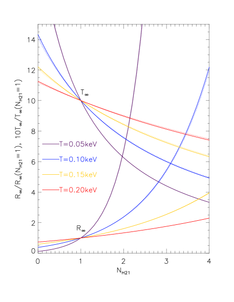
The increase of inferred with increasing is quite sensitive to the temperature. Fig. 2 shows these changes for different base effective temperatures. The dotted curves show the approximate analytic results using Eqs. (6), (10), and (11). It can be seen that, despite the nearly linear relation between and deduced by G13 for NGC 6397 and Cen, the linearity is accidental. In summary, the effects of appreciably changing are magnified by relatively low effective temperatures, and furthermore are large only for highly obscured sources (i.e., for ).
3.3 Helium Atmosphere
The case of a helium atmosphere follows similarly to that of the hydrogen case. As in the case of hydrogen, we expect that electron scattering opacities dominates the mean free path so the effective exponent can be assumed for the spectral shape. Suleimanov, Poutanen & Werner (2011) computed an array of spectral energy distributions of hydrogen and helium atmospheres as functions of temperature and gravity. Although these tables do not extend to temperatures below about 0.3 keV, comparison shows, for a given gravity, that helium atmospheres with temperatures approximately 13% smaller than hydrogen atmospheres have nearly identical energy distributions and peak energies. Therefore, a simple approximation to a helium atmosphere would be that of Eq. (9) with instead of 1.35. In this case, fitting an observed spectrum with a helium, rather than a hydrogen, atmosphere, and requiring that the peak in the energy distribution remain unaltered, leads to an inferred temperature decrease by 13% and a corresponding inferred radius increase by about 28%.
For comparison, Catuneanu et al. (2013) analyzed data from Chandra, XMM and ROSAT for the M13 QLMXB using hydrogen and helium atmospheres. They determined that fits with helium atmospheres resulted in increases in radiation radii by a factor of approximately 1.25. However, because the helium fit involved a reduction in surface gravity, and as we show below, the effective value of depends slightly on the assumed gravity, part of this radius change can be attributed to gravity effects. In contrast, Servillat et al. (2012) analyzed data for the M28 QLMXB and reported an increase in of approximately 50% for a helium instead of hydrogen atmosphere. Their helium fit also resulted in a lower gravity than the hydrogen fit. In addition, it could be expected that the relative inferred radius change could also be a function of . Exploring this in detail is beyond the scope of our analytic model. We simply assume, for the calculations described below, that a change in atmospheric composition, at fixed gravity, from hydrogen to helium results in a radiation radius increase of approximately 33%. Therefore, we expect our simulations describing the effects of considering He atmospheres to be even more qualitative than those of varying distance or . At fixed redshift, any inferred radius change will necessarily result in a gravity change.
3.4 Dependence on Gravity and Redshift
To lowest order, hydrogen and helium atmospheres have a relatively weak dependence on gravity. The effects of gravity can be modeled as a small modification to the parameter in Eq. (9). Without any temperature or gravity dependence in either or , the total integrated flux would be proportional to , and after applying a source redshift, the observed flux becomes proportional to which is the redshift-independent blackbody result. The net dependence on gravity stemming from gravity and temperature dependencies in and allow, in principle, gravity or redshift information to be deduced from the spectrum.
The array of atmospheres computed by Suleimanov, Poutanen & Werner (2011) allows an estimate of the effect of gravity to be made. For the lowest temperatures they model, the effect of gravity on the spectral distributions for hydrogen atmospheres can be approximated with a gravity-dependent parameter:
| (13) |
A similar change in the factor for helium atmospheres is found. This gravity dependence is sufficiently weak that, to lowest order, it is safely ignored for the semi-analytic approximations discussed below. In support of this thesis, we note that in the comparison made by Servillat et al. (2012), replacing hydrogen by helium resulted in an increase in of about 50% but a reduction in of only 4%.
In any case, other information in addition to the peak energy and total flux, such as higher spectral moments, need to be considered in order to be able to obtain redshift constraints from spectral fitting. This accounts for the relatively large uncertainties in redshift estimated by G13 (Table 2). We will use the original values for as computed by G13 when varying . Nevertheless, these approximations make our analysis qualitative in nature, and moderate changes to inferred neutron star properties can be expected from a more sophisticated analysis.
3.5 Calibration of the Semi-analytic Model
We now proceed to test and calibrate the predictions of the analytic model for variations in absorption by comparing to the atmosphere simulations performed by G13. G13 performed this exercise for the neutron stars in NGC 6397 and Cen. They compared the optimum values of obtained for values determined through spectral fitting and the values they attributed to Dickey & Lockman (1990). We summarize this exercise in rows 7 and 8 of columns 2-6 of Table 3, where the subscript 1 refers to G13’s value and 2 refers to values they attributed to Dickey & Lockman (1990) for the sources in NGC 6397 and Cen. Columns 7 and 8 of these rows show the results of the analytic model.
| Source | (eV) | (eV) | (eV) | |||||
|---|---|---|---|---|---|---|---|---|
| Semi-analytic model | ||||||||
| example (see text) | 100 | 0.9 | 1.8 | — | — | 78 | 2.3 | 1.8 |
| 4U 2129+49 [1] | 2.8 | 1.7 | ||||||
| 4U 1608-522 [2] | 8.0 | 15.0 | ||||||
| Cen X-4 [2] | 0.55 | 2.0 | ||||||
| Aql X-1 [2] | 2.0 | 4.0 | ||||||
| Aql X-1 [2] | 4.0 | 8.0 | ||||||
| NGC 6397 [3] | 0.96 | 1.4 | 64 | |||||
| Cen[3] | 1.82 | 0.9 | 87 | |||||
Further indication that our approximate study qualitatively predicts the effects of varying can be found in studies of quiescent X-ray binaries in the field. For example, Rutledge et al. (2000) studied the effects of varying in spectral modeling of the source 4U 2129+47 and Rutledge et al. (1999) similarly studied the sources 4U 1608-522, Cen X-4 and Aql X-1, as summarized in Table 3. It is interesting that the semi-analytic model accurately predicts the changes in effective temperatures accompanying variations in absorption. Predicted radius changes are much less accurate, but given that 90% confidence intervals for the reported radius ratios can be greater than %, the agreement is satisfactory.
| Source | (eV) | (km) | set | (eV) | ||||
|---|---|---|---|---|---|---|---|---|
| M28 | 2.52 | 119 | D90 | 131 | 0.756 | 0.830 | ||
| H10 | 116 | 1.099 | 1.065 | |||||
| NGC 6397 | 0.96 | 76 | D90 | 64 | 1.73 | 1.44 | ||
| H10 | 71 | 1.398 | 1.25 | |||||
| M13 | 0.08 | 86 | D90 | 80 | 1.20 | 1.13 | ||
| H10 | 83 | 1.17 | 1.11 | |||||
| Cen | 1.82 | 64 | D90 | 82 | 0.433 | 0.572 | ||
| H10 | 81 | 0.350 | 0.496 | |||||
| NGC 6304 | 3.46 | 106 | D90 | 118 | 0.713 | 0.80 | ||
| H10 | 104 | 1.10 | 1.07 |
Our relatively simple representation of H atmospheres is seen to overpredict the changes in radii due to variations in column density when compared to the results of G13 for the sources in NGC 6397 and Cen. This is not surprising, given that we have approximated absorption as being due to H rather than to heavier elements. However, it is clear that taking the 2/3 power of our predicted scaling factors rather closely represents the results of G13 for these sources, as displayed in the last column of Table 3. In fact, this procedure still fits the other radius ratios listed in Table 3 at the 90% confidence level. Our final procedure for the generation of alternate probability distributions is therefore to rescale the and coordinates of the probability distributions shown in Figure 1 by the power of the amount predicted from Equation (5) for the values for each source from either D90 or H10 (also using G13’s values for ). Our analytical model does not allow us to predict the value . Nevertheless, our general conclusions are not sensitive to this power, at least in the range of 1/2 to 3/2, since the ratios for different models have no dominant trend.
4 VARIATIONS OF X-RAY ABSORPTION, DISTANCE AND ATMOSPHERIC COMPOSITION
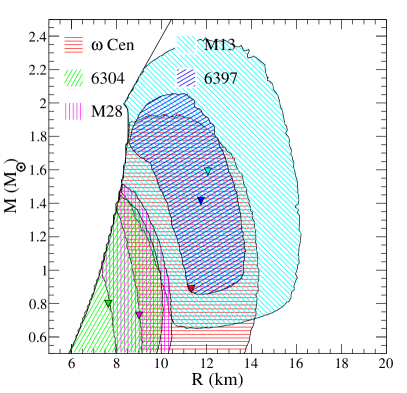
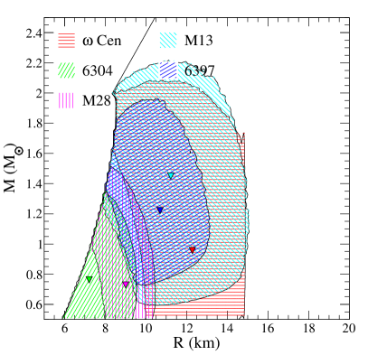
We use the final procedure described in §3.5 to modify the predicted radiation radii and probability distributions from G13 for the D90 values (left panel of Fig. 3), and for the H10 values (right panel of Fig. 3). (See Appendix B for some additional details on how the correction is applied for Cen.) The scaling factors are explicitly displayed in Table 4 for the two alternative assumptions.
There are few discernible trends in the values of for the three cases, except for the fact that the average value from D90 is about 20% smaller than that of G13 and about 20% larger than that of H10. The H10 values are larger than the G13 values in four of the five sources; the D90 values are larger than the G13 values in two of the five sources. As noted before, the H10 values are closer to the G13 values in all cases except for Cen. The average radius of the five sources for the three sets are predicted to be within about 1 km of one another. The major differences between using the D90 and H10 values occurs for M28 and NGC 6304 which have larger radii in the H10 case. Indeed, for the D90 case, NGC 6304 appears to have relatively small values of and . Nevertheless, Fig. 3 shows that, in either case D90 or H10, the new radii implied by the adjusted values are more consistent than the radii determined by G13 with the expectation that all neutron stars have similar radii, as suggested by the results of Steiner, Lattimer & Brown (2010) and Steiner, Lattimer & Brown (2013).
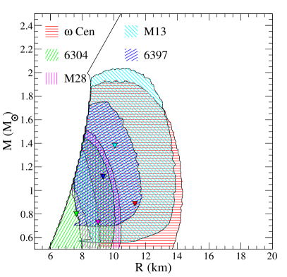
We also employ different distance measurements, and this variation is studied in Fig. 4. These results assume the values from D90 and are thus to be compared with the left panel from Fig. 3. There is some variation in the implied values of , particularly for M13 and NGC 6397. Nevertheless, the different distances give rise to smaller variations than do the different values of , and the probability regions generally overlap as long as one of the alternative sets are used.
The radius uncertainties in the above analysis could be underestimated because it is possible that one or more of these QLMXB sources have helium, rather than hydrogen, atmospheres. Ultracompact binaries, which have neutron stars that have accreted helium or carbon atmospheres from white dwarf companions, are more likely to be found in globular clusters than in the field (Deloye & Bildsten, 2004; Ivanova et al., 2008). Only in the cases of the neutron star in Cen (Haggard et al., 2004), X5 in 47 Tuc (Heinke, Grindlay & Edmonds, 2005) and several field sources has it been confirmed that the atmosphere is hydrogen. Sources with abnormally small inferred values of could have helium, rather than hydrogen, atmospheres.
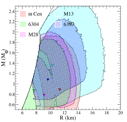
As discussed in §3.3, we approximate the effect of a helium atmosphere relative to a hydrogen atmosphere by scaling the coordinates of the probability distributions of Figure 3 and the values of of column 6 of Table 2 by a further factor of 4/3 for all of the neutron stars except that in Cen. We then add the He atmosphere probability densities to those for the hydrogen atmosphere to get the full distribution which allows for either composition. For the case of D90 values and G13 distances, the and probability distributions are shown in Fig. 5. In the cases that is sufficiently well determined by either assumed composition, as in the case of M28, this gives a visibly bimodal form to the distribution. We assume that hydrogen or helium atmospheres are equally probable, so the integrals of the probability density are equal. The helium region is broader because a larger range for gives a larger mass range, so the peak of the helium region must be lower.
5 EQUATION OF STATE AND CURVES FROM QLMXB DATA
We now analyze the QLMXB data using the Bayesian method described in Steiner, Lattimer & Brown (2010, 2013). In this analysis, the inferred probability distributions for these sources are confronted with additional constraints imposed by the assumption that the sources are neutron stars whose masses and radii are not free to vary independently but are related through the relativistic equations of stellar structure and contain a well-understood hadronic crust (the stellar region with densities below about g cm-3). In addition, we impose the constraints that the EOS is everywhere causal (i.e., that the speed of sound cannot exceed the speed of light) and . The EOS at densities higher than those of the crust is divided into three regions. The baryon properties of the lowest of these density regions is described by an expansions of the nucleon energy per baryon in density and neutron excess around and isospin symmetry. Electrons are treated as relativistic and degenerate, with the composition (i.e., the electron and proton fractions) determined by beta equilibrium. In the baseline model, the uppermost two density regions are described with polytropes (the model used in Steiner, Lattimer & Brown (2010) and also called model A in Steiner, Lattimer & Brown (2013)) that define the pressure as a function of energy density in beta equilibrium. This model is appropriate for neutron stars without strong phase transitions and is labeled “Base” below. For neutron stars with strong phase transitions due to the appearance of exotic matter, such as from a quark-hadron phase transition, we instead employ discrete line segments in the pressure–energy density plane (model C in Steiner, Lattimer & Brown (2013) and labeled “Exo” below). The assumed division of the high-density EOS into three regimes is amply justified: Read et al. (2009) has demonstrated that the detailed EOS of a wide variety of strong interaction models is accurately predicted by three polytropic segments. In either case (Base or Exo), the theoretical uncertainties in the crustal EOS produce insignificant changes to our conclusions. We also constrain neutron stars to be more massive than , a conservative lower limit. This lower limit can be justified theoretically, but it should be noted there is no significant observational evidence for the existence of neutron stars with less than .
In contrast, in their joint analysis of the five QLMXB sources, G13 did not allow the radii of the five individual neutron stars to freely vary: a common value was determined by optimizing the spectral fits to observational data. In their procedure, the correlations between masses and radii resulting from the stellar structure equations were not taken into account, and the strong constraints available from knowledge of the low-density crust EOS and causality were not considered. The lower limit to the neutron star mass was taken to be . G13 indirectly made use of the constraint that in that they justified their assumption of a near-constant radius on the grounds that the discovery of neutron stars favors interiors composed of ”normal matter”, rather than ”quark matter” or exotic matter with strong phase transitions (Lattimer & Prakash, 2010). Especially for EOSs with weak symmetry energy density dependence, i.e., EOSs predicting that have radii smaller than approximately 12 km, normal-matter stars with have less than a 10% range of radii for (Lattimer & Prakash, 2001). However, if the EOS has a strong symmetry energy density dependence, such that stars have km, the constant-radius assumption becomes less valid.
In their joint analysis of the 5 QLMXB sources under the assumption that all neutron stars have the same radius, G13 determined that the most-probable value of this radius was km when values were allowed to float and were simultaneously determined from spectral fits. In the case that values were frozen at the values optimized in the individual spectral fits, the joint analysis yielded a common radius of km. In both cases, the sources are determined to have optimum masses with a large variance, with masses ranging from to when is frozen, (Run 4 in G13) which would require either a large variation of neutron star birth masses or a large amount of accretion. It is interesting that these radii are relatively small compared to the simple average (11.3 km) of the individual best-fit radii. Partly, this is due to the fact that G13 weighted the contributions of individual sources according to the quality of data from each source. The source with the smallest inferred radius (NGC 6397) contained 35% of the total weight while the source with the largest inferred radius ( Cen) contained 7.9% of the total weight. With this unequal weighting, the average radius is reduced to 9.8 km. This is, however, still larger than the common radii G13 determined (although marginally consistent to 90% confidence with the result from their ’floating ’ analysis).
There is a straightforward explanation of this result. The values of and determined for the 5 QLMXBs in either joint analysis are not significantly different from their values determined in the individual spectral fits. is more accurately determined than . If the values of are kept fixed for each source, with the values determined in the individual spectral fits, values of the orthogonal variable change to force a common radius . This suggests that one could estimate the common radius, , for the 5 QLMXBs by minimizing the function
| (14) |
with respect to , where is the weight associated with source , and the values of the individual fits for , and the 90% confidence interval for of the th source, are and , respectively. Given the definition
| (15) |
minimization leads to
| (16) |
or, solving for ,
| (17) |
Note that normalizations associated with the Gaussian distributions in Equation (14) will cancel from Equation (16). Taking values for and from G13, and from Figure 1, we find the common radius to be km. This value is in excellent agreement with G13’s value ( km) when is frozen.
An advantage of our Bayesian analysis is that it permits one to compare in an unbiased way the quality of models with different prior assumptions in terms of their fits to the observations. We can, for example, compare models assuming normal-matter neutron stars as opposed to quark matter stars. Or, we can compare models with different assumptions about absorption, distance and composition. In addition, our analysis leads to an explicit prediction for the curve, so that the validity of the constant-radius assumption can be ascertained. In the context of Bayesian statistics, a commonly accepted way of comparing two models is through the use of Bayes factors. Given a particular model, , we can define the integral (sometimes called the evidence) as
| (18) | |||||
where is the conditional probability determined by the data and is the number of parameters (denoted ) in the EOS parameterization. This notation is defined and further discussed in Steiner, Lattimer & Brown (2010). The outer integrations are over the neutron star masses (in this case, for five objects). (This integral is simplified because we assume uniform priors in both the EOS parameters and the neutron star masses.) The Bayes factor for comparing two possible models and is then . Typically, a Bayes factor of 3 would represent “substantial” evidence that model is preferred to model , a Bayes factor of 10 would be “strong evidence”, and 100 would be “decisive” for model over . Values less than one give the opposite conclusion, e.g. a Bayes factor less than 1/10 would be strong evidence for model over .
| Model | Dist. | Comp. | (km) | ||
|---|---|---|---|---|---|
| Base | G13 | G13 | H | 11.1111.88 | (1.77 0.09) |
| Base | G13 | G13 | H+He | 11.3612.84 | (4.50 0.21) |
| Base | G13 | Alt | H | 10.7311.65 | (1.86 0.18) |
| Base | G13 | Alt | H+He | 11.4513.32 | (3.71 0.21) |
| Base | G13 | H10 | H | 10.7711.71 | (1.23 0.09) |
| Base | G13 | H10 | H+He | 11.3613.44 | (4.28 0.35) |
| Base | D90 | G13 | H | 10.6711.51 | (4.65 0.48) |
| Base | D90 | G13 | H+He | 11.3112.64 | (2.14 0.19) |
| Base | D90 | Alt | H | 10.8511.79 | (9.40 1.22) |
| Base | D90 | Alt | H+He | 11.3712.61 | (4.06 0.36) |
| Base | D90 | H10 | H | 10.7811.70 | (4.78 0.73) |
| Base | D90 | H10 | H+He | 11.2312.62 | (1.57 0.07) |
| Base | H10 | G13 | H | 10.8711.82 | (1.04 0.08) |
| Base | H10 | G13 | H+He | 11.1512.38 | (1.84 0.12) |
| Base | H10 | Alt | H | 11.0312.07 | (1.39 0.20) |
| Base | H10 | Alt | H+He | 11.0412.31 | (1.44 0.10) |
| Base | H10 | H10 | H | 10.7811.95 | (7.52 0.65) |
| Base | H10 | H10 | H+He | 11.3112.66 | (5.30 0.22) |
| Exo | G13 | G13 | H | 9.1510.81 | (7.32 0.63) |
| Exo | G13 | G13 | H+He | 10.5211.77 | (4.46 0.38) |
| Exo | G13 | Alt | H | 10.4211.39 | (1.21 0.19) |
| Exo | G13 | Alt | H+He | 10.8812.59 | (7.33 0.78) |
| Exo | G13 | H10 | H | 10.6111.41 | (2.23 0.48) |
| Exo | G13 | H10 | H+He | 10.7612.38 | (1.67 0.16) |
| Exo | D90 | G13 | H | 9.3910.97 | (5.46 1.74) |
| Exo | D90 | G13 | H+He | 10.5312.45 | (2.29 0.13) |
| Exo | D90 | Alt | H | 9.8611.44 | (3.04 0.42) |
| Exo | D90 | Alt | H+He | 10.9012.31 | (4.46 0.22) |
| Exo | D90 | H10 | H | 9.6011.38 | (2.27 0.50) |
| Exo | D90 | H10 | H+He | 10.6112.28 | (2.59 0.15) |
| Exo | H10 | G13 | H | 9.8711.49 | (5.15 0.51) |
| Exo | H10 | G13 | H+He | 10.6011.99 | (4.67 0.46) |
| Exo | H10 | Alt | H | 10.4511.74 | (5.17 0.64) |
| Exo | H10 | Alt | H+He | 10.5311.81 | (7.49 0.75) |
| Exo | H10 | H10 | H | 10.4211.72 | (2.83 0.21) |
| Exo | H10 | H10 | H+He | 10.7412.39 | (8.93 0.47) |
Note. — The first four columns give the model designations, the next column gives the posterior 90% confidence limits for the radius of a 1.4 solar mass neutron star, and the last column gives the “evidence”, the integral necessary to compute the Bayes factor.
5.1 The Simulations
The chief results of our simulations with different prior assumptions regarding column densities, distances, atmosphere composition, and the high-density EOS are given in Table 5 in terms of the predicted radii of stars and the evidence integral I for comparing models. Uncertainties in are due to the interpolation used in the integration. The three choices of column density sets are those from G13, D90, and H10. The three choices of distance sets, as described in §2, are those from G13, the ”Alt” set, and H10. The two assumed atmosphere compositions are H and the possibility of either H or He. Finally, the two assumptions for the high-density EOS are that they are given by polytropes, which represent matter without a strong phase transition, labeled ”Base”, or by four line segments, which represent matter with strong phase transitions typical of EOSs which contain exotic matter. Thus, there are a total of 36 simulations.
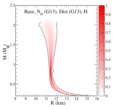
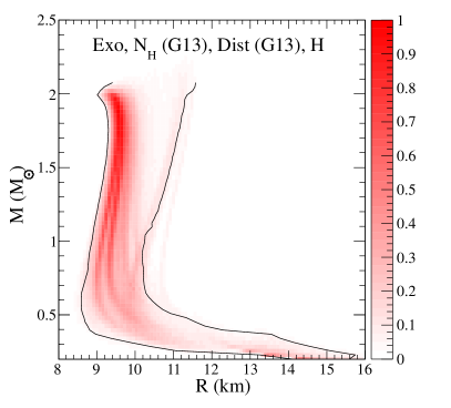
The first row in Table 5 assumes distances, column densities, and the H atmosphere composition following the assumptions of G13, slightly modified by folding in the distance uncertainty and also removing probability regions excluded by causality and the condition (Figure 1). The high-density EOS is assumed to be described by two polytropes. The radius probability distribution as a function of mass found by our Bayesian analysis is displayed in the left panel of Fig. 6. The range of radii for stars is also shown in Table 5 and is km for this case. This radius range is largely outside the 90% confidence range determined by G13 under the assumptions that (i) the radii of all sources are equal and (ii) values are allowed to float. This range is also completely outside the 90% confidence range found by G13 when values are frozen. We attribute this, in part, to the implicit use of the stellar structure equations and incorporation of a crustal EOS in our simulation and partly due to the weighting G13 assigned for each source.
| Model A/Model B | Bayes factor of A in favor of B |
|---|---|
| Base/Exo | 4.73 0.20 |
| (H10)/(D90) | 1.57 0.09 |
| (H10)/(G13) | (1.17 0.09) |
| D(Alt)/D(G13) | 1.82 0.13 |
| D(H10)/D(Alt) | 1.05 0.06 |
| H+He/H | 6.44 0.49 |
Note. — The Bayes factors comparing various scenarios, computed by forming ratios of sums of the relevant rows from Table 5. Jeffrey’s scale for the Bayes factor suggests that values greater than 3 represent “substantial” evidence, values greater than 10 represent “strong” evidence, and values greater than 100 represent “decisive” evidence for the model in the numerator as compared to the model in the denominator.
However, the set of assumptions used in the first line of Table 5 represents a model with a relatively poor fit to the data (the evidence integral for this case is 10 orders of magnitude smaller than for the most-favored cases). This is caused by the fact that the distributions found in the joint analysis for the sources in Cen and NGC 6397 are well outside their most probable regions when individually analyzed (compare our Figure 1 or Figures 4 – 8 in G13 with Figures 9 – 16 in G13). For example, the most probable mass for the neutron star in Cen is driven in the joint analysis to 2 and the radius to 10 km, just at the edge of the region allowed by causality, compared to 1.6 and 20 km, respectively, in its individual analysis.
Our results for this case but assuming an exotic matter EOS (right panel of Fig. 6, model “Exo”) imply smaller radii, km for a star, because of the presence of strong phase transitions (as observed in Steiner, Lattimer & Brown (2013)). The evidence integral, , is more than two orders of magnitude larger than the model without strong phase transitions, . This suggests that if the G13 model for X-ray absorption and distance is correct, dense matter is likely to exhibit some sort of strong phase transition. In order to make a less model-dependent statement about phase transitions, however, we should look at the ratio of the sums of the evidence integrals for all the 18 cases denoted “Base” in Table 5 and all evidence integrals for all 18 cases denoted “Exo”. This ratio is reported in the top row of Table 6 as 4.7. Thus, over all combinations of assumptions of distances, values, and atmosphere compositions, models without strong phase transitions are moderately favored. This is opposite to the above conclusion obtained from examining only one model, highlighting the importance of considering several models before making a definitive conclusion.
5.2 Alternate and Alternate Distance Simulations
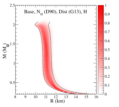
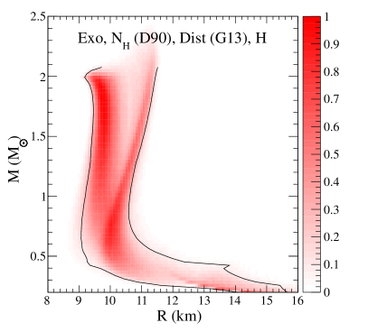
We now consider models with the alternative assumptions concerning . For the case of the D90 values, the corresponding curves, after having modified according to the prescription described in §4, are displayed in Fig. 7. We again find that the assumption of an EOS with strong phase transitions leads to smaller predicted radii than for the Base EOS. The average difference in radii is about 0.5 km, but the 90% confidence range is more than doubled in the Exo case.
After allowing for any of the distance sets, EOS models, and atmosphere compositions (with the exception of Cen), the Bayes factor for H10 in favor of D90 is 1.57 (Table 6), showing no strong preference between the two models. However, the Bayes factor for H10 in favor of G13 hydrogen column densities is over 1000. This demonstrates that, unless there is some other important model uncertainty which we have not considered, the set of X-ray absorptions determined by G13 appears ruled out. We also find little evidence to suggest that any of the three distance sets is preferred as the associated Bayes factors are all of order unity, as shown in fourth and fifth rows of Table 6.
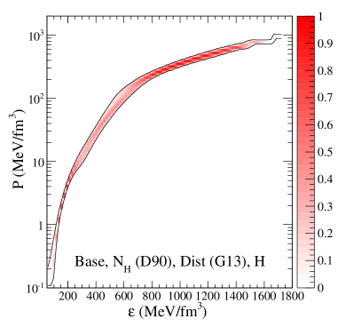
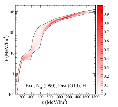
The Bayesian analysis not only leads to a predicted curve for each set of assumptions concerning the underlying EOS, distance and absorption, but also allows the prediction of the EOS parameter and the resulting pressure–energy density relation. Since our preferred Base and Exo models always prefer alternate values of , we compare such Base and Exo predictions for the EOS in Fig. 8. Both figures show the 90% confidence limits. The kinks in the pressure-density relation for the Exo model are the result of phase transitions which allow the radius to be smaller for low-mass neutron stars.
5.3 Simulations with both H and He Atmospheres
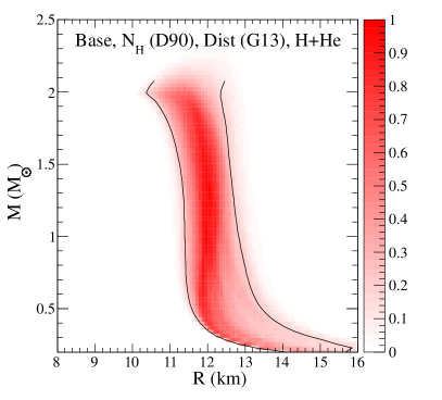
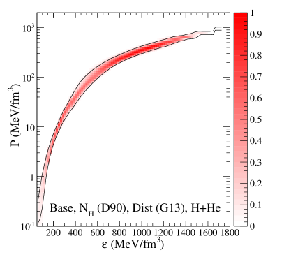
Our results indicate there is evidence that at least one of the neutron stars other than Cen has a helium atmosphere. This assertion is supported by the overall Bayes factor for the H+He in favor of the H models, which is 6.4, as given in the last row of Table 6. In the particular case where there are no strong phase transitions, the values are given by D90, and the distances are taken from G13, the Bayes factor is considerably larger, . The associated EOS and curves are given in Fig. 9, and the radius of a 1.4 neutron star is between 11.31 km and 12.64 km. For the H10 values of , the Bayes factor is about 180 and the predicted radius range is about 0.3 km lower. In either case, these radii are similar to those that one expects from the PRE X-ray sources (Steiner, Lattimer & Brown, 2013). However, these conclusions depend on assumptions about . If a future study were to confirm even larger values of for M28 and NGC 6304 than those of H10, then the evidence for helium atmospheres would become weaker.
6 DISCUSSION AND CONCLUSIONS
Our results show that models employing independently determined values for are strongly favored over models that use values self-consistently derived as part of the spectral fitting procedure. We also find that allowing the possibility of either hydrogen or helium atmospheres is strongly favored by the currently available mass and radius data from QLMXBs. In this case, the combination of independently-determined values with the possibility of either H or He atmospheres, there is substantial evidence that the EOS of dense matter does not have a strong phase transition, such as those due to the quark-hadron phase transition. However, if all sources are eventually shown to possess hydrogen atmospheres, the EOS is then favored to have strong phase transitions. For our Base EOS and over all assumptions about distance, absorption, and atmosphere composition, the models which have the largest value of the evidence integral, , suggest that the radius of a neutron star is predicted to be between 11.15 and 12.66 km. For the Exo EOS, the models which have the largest evidence, , give smaller radii, between 10.45 and 12.45 km. Both of these ranges are consistent with the predicted radius range for stars from nuclear experimental (Newton et al., 2011; Tsang et al., 2012; Lattimer & Lim, 2013) and theoretical neutron matter studies (Steiner & Gandolfi, 2012; Hebeler et al., 2013), about 10.7–13.1 km and 9.7 – 13.9 km, respectively, with all confidence regions being 90%.
However, the uncertainties in might be quite large. The analysis from G13 suggests that the ratio of values determined from spectral fitting to those from HI surveys can range from 1/2 to 2. In the context of mass and radius observations, this uncertainty has enormous implications. Our work should motivate more extensive observations in several wavelength regimes to determine along the lines of sights to globular clusters with more precision. In the radio, more detailed measurements of HI column densities and metallicities of intervening matter are possible with present technologies. In X-rays, however, the problem is more challenging because large throughput detectors with high spectral resolution at low energies (0.1 - 0.3 keV) are required to determine column densities directly through observations of edges in the spectrum. It is possible that observations of bright X-ray bursts from these clusters could provide the required information. The absolute flux calibration of X-ray detectors could also shift radius measurements in either direction by as much as 15%. Distance uncertainties are still as large as 25% and should be improved. Better X-ray data is needed to determine the atmosphere compositions of accreting neutron stars in QLMXB systems, as this can make 30% or greater changes in inferred neutron star radii. In addition observations of H emission could help pin down atmosphere compositions. The relative normalizations of the QLMXB distributions could be varied and such variation will change the Bayes factors and the associated interpretation. These normalizations will be additionally confounded by systematics which are common to all sources, such as those which result from the slow decay of X-ray observing instruments.
There are also systematic uncertainties in the probability distributions for neutron star radii, the EOS, and for the Bayes factors coming from the choice of the prior distribution. The choice of prior manifests itself in two ways: the selection of the EOS parameterization, and the choice of the neutron star mass function. The effect of the EOS parameterization could be analyzed more systematically, e.g. through a hierarchical analysis, but this would require a large computational effort beyond the scope of this work. The neutron star mass function could also be varied, in line with recent progress in mass measurements (Lattimer, 2012) and this will be pursued in future work. Assuming that neutron stars of low mass are more probable will tend to prefer smaller values of , because causality and the maximum mass constraint tend to prefer curves which are vertical (i.e. fixed ) in the region of interest. This could provide evidence in favor of strong phase transitions and H atmospheres.
The thesis that low-mass X-ray binary systems studied here contain strange quark stars rather than neutron stars could be consistent with the relatively small range of redshifts and small radii obtained for some of the QLMXBs especially if our alternate values are correct for Cen. On the other hand, it is difficult for strange quark stars to reproduce the wide array of phenomenology observed in LMXBs including X-ray bursts, superbursts (Page & Cumming, 2005), and crust cooling (Stejner & Madsen, 2006). Furthermore, if the neutron star maximum mass is substantially higher than , as perhaps indicated by the two black widow pulsar systems PSR B1957+20 (van Kerkwijk, Breton and Kulkarni, 2011) and PSR J1311-3430 (Romani et al., 2012), as well as the binary pulsar J1748-2021B in NGC 6440 (Freire et al., 2008), the possibility of strange quark stars is strongly disfavored.
This work is supported by DOE grants DE-AC02-87ER40317 (J.M.L.) and DE-FG02-00ER41132 (A.W.S.). This work used the resources of the National Energy Research Scientific Computing Center (NERSC), which is supported by the Office of Science of the U.S. Department of Energy under Contract No. DE-AC02-05CH11231. We thank E. Brown, S. Gandolfi, S. Guillot and S. Reddy for discussions, S. Gandolfi for help with the NERSC computations, S. Guillot for providing data from G13, and E. Brown bringing to our attention the analytic approximation for hydrogen atmospheres, Eq. (9), and its derivation in Appendix A.
APPENDIX A: Justification for the Value
To justify that , consider the competition between scattering and absorption in a hydrogen atmosphere. The electron scattering cross section is constant and, for energies near the peak of the spectrum, is much greater than the free-free cross section , which depends on energy, density and temperature as . The total distance a photon travels before being absorbed is approximately where is the respective mean free path and is the number density of electrons. For a random walk, the physical depth a photon travels before being absorbed is .
To allow for changes in density and temperature in the atmosphere, emerging photons of energy originate from an approximate depth determined by
| (19) |
where is Avogadro’s number and is the mean molecular weight per electron. From hydrostatic equilibrium, where is the constant surface gravity and is the pressure. For a gray atmosphere, . Eq. (19) can thus be expressed as
| (20) |
Therefore, the temperature at the depth where emergent photons of energy originate scales with energy as . For a Planckian spectrum at large optical depths, the specific flux therefore behaves like
| (21) |
Calibrating the peak flux to model hydrogen atmospheres (Romani, 1987; Zavlin, Pavlov & Shibanov, 1996) allows determination of the specific flux in this approximation,
| (22) |
where and are in keV. Another analytic approximation was determined by McClintock, Narayan & Rybicki (2004), which is
| (23) |
where . Our approximation represents a better fit for K, which suggests an improved approximation might be found if was a monotonically increasing function of temperature. However, most of the sources under study have K, so we forgo a better approximation and simply utilize Eq. (22) in the subsequent discussion. A simplification afforded by either of Eqs. (22) or (23) is that effects of gravity will be straightforward to approximate, which ceases to be the case when is a temperature-dependent parameter.
APPENDIX B: Rescaling for the Neutron Star in Cen
G13 obtained a large value for in the case of Cen because they deduced a large value for . Their probability distributions were confined to , which effectively decreases to when is corrected by the factor of 0.511 for our lower alternative value of as given in Table 2. This results in missing information which creates an unphysical constraint on the mass of the neutron star when computing the corrected distribution. We therefore simulate data for in this case using the same distribution in and as that inferred from G13 in the region km, the region unaffected by the limit. The simulated data is added to the original G13 data and the sum is renormalized to ensure that the probability distribution is smooth across the boundary.
References
- Antoniadis et al. (2013) J. Antoniadis, P. C. C. Freire, N. Wex, et al., Science 340, 448 (2013)
- Becker et al. (2003) W. Becker, D. A. Swartz, G. G. Pavlov, R. F. Elsner, J. Grindlay, R. Mignani, A. F. Tennant, D. Backer, L. Pulone, V. Testa and M. C. Weisskopf, ApJ, 594, 798 (2003)
- Bildsten, Salpeter & Wasserman (1992) L. Bildsten, E. E. Salpeter and I. Wasserman, ApJ 384, 143 (1992)
- Brown, Bildsten & Rutledge (1998) E. F. Brown, L. Bildsten and R. E. Rutledge, ApJ Lett. 504, L95 (1998)
- Campana et al. (1998) S. Campana, M. Colpi, S. Mereghetti, L. Stella and M. Tavani, A&ARv 8, 279 (1998)
- Catuneanu et al. (2013) A. Catuneanu, C. O. Heinke, G. R. Sivakoff, W.C. G. Ho, and M. Servillat, ApJ 764, 145 (2013)
- Deloye & Bildsten (2004) C. J. Deloye and L. Bildsten, ApJ Lett. 607, 119 (2004)
- Demorest et al. (2010) P. B. Demorest, T. Pennucci, S. M. Ransom, M. S. E. Roberts and J. W. T. Hessels, Nature 467, 1081 (2010)
- Dickey & Lockman (1990) J. M. Dickey and F. J. Lockman, ARA&A 28, 215 (1990)
- Freire et al. (2008) P. C. C. Freire, S. M. Ransom, S. Bégin, I. H. Stairs, J.W. T. Hessels, L. H. Frey and F. Camilo, ApJ 675, 670 (2008)
- Fridriksson et al. (2010) J. K. Fredriksson, J. Homan, R. Wijands, M. Méndez, D. Altamirano, E. M. Cackett, E. F. Brown, T. M. Belloni, N. Degenaar and W. H. G. Lewin, ApJ 714, 270 (2010)
- Gendre, Barret & Webb (2003a) B. Gendre, D. Barret and N. A. Webb, A&A 400, 521 (2003a)
- Gendre, Barret & Webb (2003b) B. Gendre, D. Barret and N. A. Webb, A&A 403, L11 (2003b)
- Gratton, et al. (2003) R. G. Gratton, A. Bragaglia, E. Carretta, G. Clemntini, S. Desidera, F. Grundahl, and S. Lucatello, A&A 408, 529 (2003)
- Guillot et al. (2009) S. Guillot, R. E. Rutledge, L. Bildsten, E. F. Brown, G. G. Pavlov and V. E. Zavlin, MNRAS 392, 665 (2009)
- Guillot, Rutledge & Brown (2011a) S. Guillot, R. E. Rutledge and E. F. Brown, ApJ 732, 88 (2011a)
- Guillot et al. (2011b) S. Guillot, R. E. Rutledge, E. F. Brown, G. G. Pavlov and V. E. Zavlin, ApJ 738, 129 (2011b)
- Guillot et al. (2013) S. Guillot, M. Servillat, N. A. Webb and R. E. Rutledge, ApJ 772, 7 (2013)
- Güver & Ozel (2009) T. Güver and F. Özel, MNRAS 400, 2050 (2009)
- Güver et al. (2010a) T. Güver, F. Özel, A. Cabrera-Lavers and P. Wroblewski, ApJ 712, 964 (2010)
- Güver et al. (2010b) T. Güver, P. Wroblewski, L. Camarota and F. Özel, ApJ 719, 1807 (2010)
- Güver & Özel (2013) T. Güver and F. Özel, ApJ 765, 1 (2013)
- Haakonsen et al. (2012) C. B. Haakonsen, M. Turner, N. A. Tacik and R. E. Rutledge, ApJ 749, 52 (2012)
- Haggard et al. (2004) D. Haggard, A. M. Cool, J. Anderson, P. D. Edmonds, P. J. Callanan, C. O. Heinke, J. E. Grindlay and C. D. Bailyn, ApJ 613, 512 (2004)
- Harris (2010) W. E. Harris, AJ 112, 1487 (1996; online table updated in 2010); http://physwww.physics.mcmaster.ca/~harris/mwgc.dat
- Hansen et al. (2007) B. M. S. Hansen, J. Anderson, J Brewer, A. Dotter, G.G. Fahlman, J. Hurley, J Kalirai, I. King, D. Reitzel, H. B. Richer, R. M. Rich, M. M. Shara and P. B. Stetson, ApJ 671, 380 (2007)
- Hebeler et al. (2013) K. Hebeler, J. M. Lattimer, C. J. Pethick and A. Schwenk, ApJ 773, 11 (2013)
- Heinke, Grindlay & Edmonds (2005) C. O. Heinke, J. E. Grindlay and P. D. Edmonds, ApJ 622, 556 (2005)
- Heinke et al. (2006) C. O. Heinke, G. B. Rybicki, R. Narayan and J. E. Grindlay, ApJ 644, 1090 (2006)
- Ho and Heinke (2009) W. C. G. Ho and C. O. Heinke, Nature 462, 71 (2009)
- Ivanova et al. (2008) N. Ivanova, C. O. Heinke, F. A. Rasio, K. Belczynski and J. M. Fregeau,MNRAS 386, 553 (2008)
- Kalberla et al. (2005) P. M. W. Kalberla, W. B. Burton, D. Hartmann, E. M. Arnal, E. Bajaja, R. Morras and W. G. L. Pöppel, A&A 440, 775 (2005)
- Koranda, Stergiolas & Friedman (1997) S. Koranda, N. Stergioulas and J.L. Friedman, ApJ 488, 799 (1997)
- Lattimer (2012) J. M. Lattimer, Annu. Rev. Nucl. Part. Sci. 62, 485 (2012)
- Lattimer & Prakash (2001) J. M. Lattimer and M. Prakash, ApJ 550, 426 (2001)
- Lattimer & Prakash (2005) J. M. Lattimer and M. Prakash, Phys. Rev. Lett. 94, 111101 (2005)
- Lattimer & Prakash (2007) J. M. Lattimer and M. Prakash, Phys. Rep. 442, 109 (2007)
- Lattimer & Prakash (2010) J. M. Lattimer and M. Prakash, in From Nuclei to Stars, ed. S. Lee (World Scientific, Hong Kong), p. 275 (2010); arXiv:1012.3208
- Lattimer & Lim (2013) J. M. Lattimer and Y. Lim, ApJ 771, 51 (2013)
- Lewin, van Paradijs & Taam (1993) W. H. G. Lewin, J. van Paradijs and R. E. Taam, Sp. Sci. Rev. 62, 223 (1993)
- McClintock, Narayan & Rybicki (2004) J. E. McClintock, R. Narayan and G. B. Rybicki, ApJ 615, 402 (2004)
- Newton et al. (2011) W. G. Newton, M. Gearheart, J. Hooker and B.-A. Li, in ”Neutron Star Crust”, ed. C. A. Bertulani and J. Piekarewicz, arXiv:1112.2018 (2011)
- Özel, Baym & Güver (2010) F. Özel, G. Baym and T. Güver, Phys. Rev. D. 82, 101301 (2010)
- Özel, Gould & Güver (2012) F. Özel, A. Gould and T. Güver, ApJ 748, 5 (2011)
- Özel, Güver & Psaltis (2009) F. Özel, T. Güver and D. Psaltis, ApJ 693, 1775 (2009)
- Page & Cumming (2005) D. Page and A. Cumming, ApJL 635, 157 (2005)
- Predehl & Schmitt (1995) P. Predehl and J. H. M. M. Schmitt, Astron. & Astrophys. 293, 889 (1995)
- Rajagopal & Romani (1996) M Rajagopal and R. W. Romani, ApJ 461, 327 (1996)
- Rappaport, et al. (1987) S. Rappaport, C. P. Ma, P. C. Joss and L. A. Nelson, ApJ 322, 842 (1987)
- Read et al. (2009) J. S. Read, B. D. Lackey, B. J. Owen and J. L. Friedman, Phys. Rev. D 79, 124032 (2009)
- Romani (1987) R. W. Romani, ApJ 313, 718 (1987)
- Romani et al. (2012) R. W. Romani, A. V. Filippenko, J. M. Silverman, S. B. Cenko, J. Greiner, A. Rau, J. Elliott and H. J. Pletsch, ApJ 760, L36 (2012)
- Rutledge et al. (1999) R. E. Rutledge, L. Bildsten, E. F. Brown, G. G. Pavlov and E. V. Zavlin, ApJ 514, 945 (1999)
- Rutledge et al. (2000) R. E. Rutledge, L. Bildsten, E. F. Brown, G. G. Pavlov and V. E. Zavlin, ApJ 529, 985 (2000)
- Rutledge et al. (2002a) R. E. Rutledge, L. Bildsten, E. F. Brown, G. G. Pavlov and V. E. Zavlin, ApJ 577, 346 (2002)
- Rutledge et al. (2002b) R. E. Rutledge, L. Bildsten, E. F. Brown, G. G. Pavlov and V. E. Zavlin, ApJ 578, 405 (2002)
- Servillat et al. (2012) M. Servillat, C. O. Heinke, W. C. G. Ho, J. E. Grindlay, J. Hong, M. van den Berg and S. Bogdanov, MNRAS 423, 1556 (2012)
- Steiner, Lattimer & Brown (2010) A. W. Steiner, J. M. Lattimer and E. F. Brown, ApJ 722, 33 (2010)
- Steiner & Gandolfi (2012) A. W. Steiner and S. Gandolfi, Phys. Rev. Lett. 108, 081102 (2012)
- Steiner, Lattimer & Brown (2013) A. W. Steiner, J. M. Lattimer and E. F. Brown, ApJ Lett. 765, 5 (2013)
- Stejner & Madsen (2006) M. Stejner and J. Madsen, A&A 458, 523 (2006)
- Stella, Priedhorsky & White (1987) L. Stella, W. Priedhorsky and N. E. White, ApJ Lett. 312, 17 (1987)
- Suleimanov, Poutanen & Werner (2011) V. Suleimanov, J. Poutanen and K. Werner, Astron. & Astrophys. 527, A139 (2011)
- Tsang et al. (2012) M. B. Tsang, J. R. Stone, F. Camera, P. Danielewicz, S. Gandolfi, K. Hebeler, C. J. Horowitz, J. Lee, W. G. Lynch, Z. Kohley, R. Lemmon, P. Moller, T. Murakami, S. Riordan, X. Roca-Maza, F. Sammarruca, A. W. Steiner, I. Vidana and S. J. Yennello, Phys. Rev. C 86, 015803 (2012)
- van Kerkwijk, Breton and Kulkarni (2011) M. H. van Kerkwijk, R. P. Breton and S. R. Kulkarni, ApJ 728, 95 (2011)
- Van Paradijs (1979) J. van Paradijs, ApJ 234, 609 (1979)
- Webb & Barret (2007) N. A. Webb and D. Barret, ApJ 671, 727 (2007)
- Wilms, Allen & McCray (2000) J. Wilms, A. Allen and R. McCray, ApJ 542, 914 (2000)
- Zavlin, Pavlov & Shibanov (1996) V. E. Zavlin, G. G. Pavlov and Yu. A. Shibanov, Astron. & Astrophys. 315, 141 (1996)