Elemental unbiased estimators for the Generalized Pareto tail

Abstract

Unbiased location- and scale-invariant ‘elemental’ estimators for the GPD tail parameter are constructed. Each involves three log-spacings. The estimators are unbiased for finite sample sizes, even as small as $N=3$. It is shown that the elementals form a complete basis for unbiased location- and scale-invariant estimators constructed from linear combinations of log-spacings. Preliminary numerical evidence is presented which suggests that elemental combinations can be constructed which are consistent estimators of the tail parameter for samples drawn from the pure GPD family.

1 Introduction

The Generalized Pareto Distribution (GPD) and the Generalized Extreme Value (GEV) distribution play a central role in extreme value theory. Each has three parameters $(\mu,\sigma,\xi)$ corresponding to location, scale and tail (or shape) respectively. This paper describes a particularly simple set of location- and scale-invariant ‘elemental’ estimators for the GPD tail parameter. Each ‘elemental’ involves three log-spacings of the data, and each is unbiased over all tail parameters $-\infty<\xi<\infty$, and for all sample sizes, as small as $N=3$.

The elemental estimators (illustrated in Figure 1) have the form

$$\hat{\xi}_{IJ}=\log\frac{\tau^{J-1}}{t^{I}}\ \ \ \text{where}\ \ \ \tau=\frac{X_{I}-X_{J-1}}{X_{I}-X_{J}}\ \ \ \text{and}\ \ \ t=\frac{X_{I+1}-X_{J}}{X_{I}-X_{J}},\ \ \text{with}\ J\geq I+2$$ (1)

and the $X_{I}$ are the upper-order statistics, numbered in decreasing order starting from $I=1$ as the data maximum.

Figure 1: Between any two non-adjacent data points $X_{I}$ and $X_{J}$ an elemental estimator $\hat{\xi}_{IJ}$ can be defined. It involves three log-spacings - the one between $X_{I}$ and $X_{J}$, together with two shorter log-spacings connecting each end-point to the data point immediately inside the other end.

The Generalized Pareto Distribution arises as the limiting distribution of maxima in Peaks-Over-Threshold approaches (see for example Embrechts et al. (1999)). It has distribution function:

$$F(x)=1-\left(1+\xi\frac{x-\mu}{\sigma}\right)^{-1/\xi}$$ (2)

The parameters $\mu$ and $\xi$ can take any value on the real line, whilst $\sigma$ can be any positive value (and when $\xi=0$ the distribution function (2) becomes the exponential distribution). For GPDs with positive $\xi$, the support ($\mu\leq x$) is unbounded at the right, giving long- or heavy-tailed distributions. For $\xi$ negative, the support is bounded both below and above ($\mu\leq x\leq\mu-\sigma/\xi$).

2 Other estimators

Estimators for the tail parameter can be loosely classed into: maximum likelihood (ML); method of moments; Pickands-like and Bayesian. Standard texts such as Embrechts et al. (1999) and Reiss and Thomas (2001) provide detailed background, with Coles (2001) giving the Bayesian perspective. de Zea Bermudez and Kotz (2010) provide a comprehensive review, such that only a brief survey is presented here.

The maximum likelihood approach to the GPD is described in Smith (1987). Although it possesses some desirable properties, the numerical maximization algorithms can experience problems for small sample sizes and for negative tail parameters, as there are occasions when the likelihood function does not possess a local maximum (Castillo and Daoudi (2009)). To avoid such problems, a method of moments approach was proposed by Hosking and Wallis (1987).

The classical tail parameter estimator is that of Hill (1975). However, it is not location invariant and is only valid in the heavy-tailed Frechét region ($\xi$ positive) of the GEV, although an extension into the Weibull region ($\xi$ negative) was proposed by Dekkers et al. (1989) using the method of moments. Pickands (1975) proposed an estimator based on log-spacings which overcame many of these shortcomings. This estimator is popular in current applications, and a substantial literature exists on its generalization (Drees (1998); Yun (2002), for example), the most general and efficient of which appear to be those of Segers (2005), derived using second order theory of regular variation. These are optimised for estimation of the tail index in the more general case of data drawn from any distribution within the domain of attraction of the particular GPD. Although the main concern of Extreme Value Theory is the domain of attraction case, this paper restricts attention to distributions within the pure GPD family. The possibility that results derived in this specific setting may be extended to the more general case is left for later consideration.

Throughout, there is an emphasis on results that are valid for small sample sizes.

3 Elemental Estimators

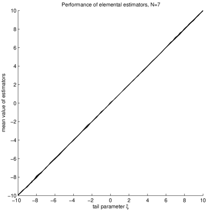
The main result here is the proof in Appendix 1 that each elemental estimator is absolutely unbiased within the GPD family. That the proof is valid, remarkably, for ALL $\xi$ may be appreciated by inspection of Eqn. 7 there. For $\xi$ negative, the expectation of the log-spacing is expressed in terms of the tail probabilities $G_{i}$ and $G_{j}$ via a term $\log(G_{j}^{\gamma}-G_{i}^{\gamma})$ with $\gamma=-\xi$. This trivially decomposes into a simple term $\gamma\log G_{j}$ and a complicated term $\log(1-(G_{i}/G_{j})^{\gamma})$. The proof shows how the simple terms provide the expectation $\hat{\xi}=-\gamma$, and how the elementals combine the complicated terms in such a manner that they cancel (obviating the need to evaluate them explicitly). For $\xi$ positive, the absolute lack of bias is maintained by an additional simple term $\gamma\log G_{i}G_{j}$ which adds $2\gamma$ to the $-\gamma$ result for $\xi$ negative. This elegant correspondence between the results for $\xi$ positive and negative is absent in previous approaches to GPD tail estimation. As further demonstration of the absolute lack of bias of each elemental triplet, even at small sample sizes, the numerically-returned average values for each of the fifteen elemental estimators available for $N=7$ are shown in Fig. 2 over a wide range of tail parameters ($-10\leq\xi\leq 10$).

Figure 2: Averages over 50,000 samples for the 15 elemental estimators for $N=7$ over a range of $\xi$. The fifteen lines are almost indistinguishable from the diagonal, indicating that each is indeed absolutely unbiased.

4 Linear combinations

Trivially, any unit-weight linear combination of elementals will also be unbiased. Whilst it will be of interest to form efficient combinations, no detailed analysis of efficiency or variance is undertaken here. Instead, the performance of a simple combination is reported.

Linear combinations of elementals are most conveniently described via the upper triangular matrix $M$ of dimension $N\times N$ of Table 2 containing all possible log-spacings. The general term is $M_{IJ}=\log(X_{I}-X_{J})$ for $J\geq I+1$ and zero otherwise. (Use of the $N\times N$ form with zero diagonal allows for easier indexing). Each element above the secondary diagonal ($J\geq I+2$) may be uniquely identified with an elemental estimator, involving that log-spacing, that to its left and that below it in $M$. Corresponding weights of elemental estimator combinations may thus be stored in an $N\times N$ upper triangular matrix $R$. Weighting an elemental $\hat{\xi}_{IJ}$ by $r_{IJ}$ requires (from Eqn. 1) that the three weights $r_{IJ}\times\{J-1,-(J-1-I),-I\}$ be given, respectively, to the corresponding left, upper-right and lower log-spacings in $M$. These weights are illustrated in the grid $G$ shown in Table 2. The totals may then be collected in an $N\times N$ matrix $A$ of log-spacing weights. The sum of the entrywise product of $A$ and $M$ is then the unbiased estimate $\hat{\xi}$.

	$\log(X_{1}-X_{2})$	$\log(X_{1}-X_{3})$	$\log(X_{1}-X_{4})$	$\log(X_{1}-X_{5})$	$\log(X_{1}-X_{6})$	$\log(X_{1}-X_{7})$
		$\log(X_{2}-X_{3})$	$\log(X_{2}-X_{4})$	$\log(X_{2}-X_{5})$	$\log(X_{2}-X_{6})$	$\log(X_{2}-X_{7})$
			$\log(X_{3}-X_{4})$	$\pagecolor[gray]{0.8}\log(X_{3}-X_{5})$	$\log(X_{3}-X_{6})$	$\log(X_{3}-X_{7})$
				$\log(X_{4}-X_{5})$	$\log(X_{4}-X_{6})$	$\log(X_{4}-X_{7})$
					$\log(X_{5}-X_{6})$	$\log(X_{5}-X_{7})$
						$\log(X_{6}-X_{7})$

Table 1: The address matrix $M$ for $N=7$. Each elemental involves three adjacent cells in an inverted-L formation. That corresponding to the elemental $\hat{\xi}_{36}$ is shaded for illustration.

			2	-1		3	-2		4	-3		5	-4		6	-5
				-1			-1			-1			-1			-1
						3	-1		4	-2		5	-3		6	-4
							-2			-2			-2			-2
									4	-1		5	-2		6	-3
										-3			-3			-3
												5	-1		6	-2
													-4			-4
															6	-1
																-5

Table 2: The grid $G$ of exponents of the elemental estimators, for $N=7$. Again, the terms involved in the elemental $\hat{\xi}_{36}$ are shaded for illustration.

In summary, the matrix $M$ is the roadmap of all log-spacings and the grid $G$ gives the set of weights to be used within each elemental. A linear combination of elementals is then defined by a unit-sum matrix $R$, and the corresponding log-spacing weights are collected in the zero-sum matrix $A$.

An example combination

A natural choice of linear combination might give equal weight to each elemental. However here we give further consideration to a simple “linearly-rising” combination. Numerical experiments indicate that many simple choices of linear combination lead to good estimators, and further research may seek the optimal combination. There is thus nothing special about the “linearly-rising” combination considered here. As will be demonstrated, it has a good all-round performance, but more importantly it illustrates the great simplicity that the elementals permit, allowing the ready creation of unbiased tail estimators with efficiencies comparable to current leading (and often highly complicated) alternatives.

The “linearly-rising” combination has elemental weights $r_{IJ}\propto N+1-J$ and the resulting log-spacing weights are $a_{IJ}=6(2N-3J+2)/(N(N-1)(N-2))$ for $J\geq I+1$. For example, for $N=7$ the weights are

$$R=\ \frac{1}{35}\left(\begin{array}[]{ccccccc}.&.&5&4&3&2&1\\ &&&4&3&2&1\\ &&&&3&2&1\\ &&&&&2&1\\ &&&&&&1\\ &&&&&&\\ &&&&&&\\ \end{array}\right)\ \ \text{giving}\ A=\ \frac{1}{35}\left(\begin{array}[]{ccccccc}.&10&7&4&1&-2&-5\\ &&7&4&1&-2&-5\\ &&&4&1&-2&-5\\ &&&&1&-2&-5\\ &&&&&-2&-5\\ &&&&&&-5\\ &&&&&&\\ \end{array}\right)$$

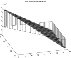
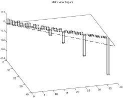
Further illustration is given in Figure 3 (centre) for a sample size of 40, showing how the log-spacing weights have a simple linearly-rising distribution with zero mean. For comparison, the unusual pattern of the corresponding log-spacing weights of an unconstrained (i.e. optimised but biased) Segers estimator are also shown. Since the Segers estimator has only a single non-zero weight in each column it immediately follows that it cannot be constructed from the elemental triplets.

Figure 3: The $A$ matrix of log-spacing weights for a typical elemental, the combined elementals and a Segers estimator.

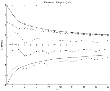
In Figure 4, the errors of the elemental combination are compared with those of the unconstrained Segers estimator for pure GPDs with the somewhat extreme cases of $\xi=\pm 3$, and small sample sizes. The elemental combination has comparatively large variance around an unbiased mean, in contrast to the Segers estimator which is more tightly bunched around a biased offset. Despite the complexity, the extensive optimization and the substantial bias in the Segers estimator, its mean square error is nevertheless typically only marginally less than that of the simple elemental combination.

Figure 4: The mean, (mean $\pm$ std. dev.), and (actual + rmse) for the elemental combination (solid lines) and the unconstrained Segers (dashed) for 10,000 samples of sizes $N=3$ to $20$ drawn from GPDs with $\xi=3$ and $\xi=-3$. Means are highlighted with $+$ and actual-plus-rmse by $\circ$. Note the large bias in the Segers estimator (particularly for $\xi=-3$), and note the lack of bias in the elemental combination for samples as small as $N=3$.

5 Completeness

Proposition: if $\hat{\xi}$ is a linear combination of log-spacings and is an absolutely-unbiased, location- and scale-invariant estimator of the tail parameter of the GPD, then $\hat{\xi}$ is a linear combination of elementals.

The proof, presented in Appendix 2, shows that a requirement for lack of bias imposes $N-1$ independent constraints on the $N(N-1)/2$ dimensional space of possible linear combinations. The resulting subspace of unbiased estimators thus has dimension $(N-1)(N-2)/2$ and is that subspace spanned by the elementals. The elementals thus form a complete basis for unbiased, location- and scale-invariant log-spacing estimators of the GPD tail parameter.

6 Efficiency and Optimality

Given that the efficiency of the estimator depends on the actual unknown value of the parameter $\xi$, there is no unique definition of optimality. The question as to which linear combination is in some sense the ‘best’ is thus a matter of judgement.

Figure 5: The relative efficiency of various linear combinations of elementals (for GPD samples of size $N=20$ over a range of $\xi$). Efficiency is defined relative to the numerically-computed minimal variance at given $\xi$ within the class of location- and scale-invariant unbiased estimators that are linear combinations of log-spacings. The linearly-rising combination $r_{ij}\propto N+1-j$ is seen to be a good compromise, giving high relative efficiency over the whole range $-3\leq\xi\leq 3$.

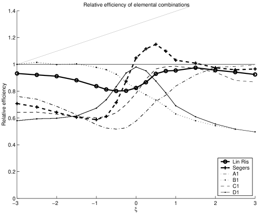
Fig. 5 shows the relative efficiency of various linear combinations of elementals, wherein relative efficiency is defined with respect to the minimal possible variance (given the tail parameter $\xi$) within the class of location- and scale-invariant unbiased estimators which are linear combinations of log-spacings of GPD data. Using the completeness of the elementals, at any $\xi$ and for any sample size $N$, the unbiased combination giving minimum variance within this class can be estimated numerically by constructing, via repeated samples, the numerical covariance matrix for the set of $(N-1)(N-2)/2$ elementals, and applying a Lagrange multiplier to enforce the unit sum condition on the coefficients $r_{ij}$. The Lagrange multiplier is then an estimate of the minimum variance. Since the computed coefficients are minimal for that set of samples, it will, for that sample set, perform better than the actual global optimum, and thus provide a lower bound on the minimum variance. The computed coefficients will not be fully optimal for other randomly drawn sample sets, and since the global optimum is, on average, optimal for other sets, then an upper bound on the minimum possible variance (within this class of estimators) can be obtained by applying the numerically-computed optimal coefficients to a large set of samples which were not used in their computation. By this procedure, using two separate blocks of 8000 samples of size $N=20$ drawn from GPDs, the (approximate) optimal linear combination within the class was constructed for various $\xi$.

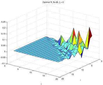
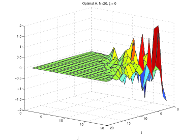
The optimal elemental coefficients $r_{ij}$ and corresponding log-spacing coefficients $a_{ij}$ computed for $\xi=0$ are shown in Fig. 6. It can be seen that the coefficients are small near the $i\approx j$ diagonal, rising in amplitude near the top corner $i\approx 1,j\approx N-2$. At all values of $\xi$ investigated, the optimal coefficients had this characteristic. Moreover all exhibited the decidedly non-smooth character reminiscent of the measure $\lambda$ in Seger’s optimisation procedure (Segers (2005)).

Figure 6: The numerically computed matrix elements $r_{ij}$ and $a_{ij}$ that minimise the variance at $\xi=0$.

Although $\xi$-specific optimal combinations have thus been computed, these are not optimal in any global sense, as their performance is far from optimal away from the values of $\xi$ at which they were optimised. This can be seen in Fig. 5, where the curve D1 shows the performance of the optimal $\xi=0$ combination falling away rapidly from perfect relative efficiency for $\xi$ values different from zero.

Fig. 5 also shows the performance of some representative examples of other linear combinations. Curve A1 is for equal elemental weights ($r_{ij}=$ constant), showing good performance in the very heavy-tailed region, but with much lower efficiency for $\xi$ small or negative.

Curve B1 has $r_{ij}\propto 1/(ii(ii+1))$, and thus gives much weight to the top row of the matrices, where log-spacings are measured from the data maximum. This combination is seen to give excellent performance in the $\xi$ negative region, but has low efficiency for $\xi$ positive.

Curve C1 (dashed) is for $r_{ij}\propto(jj-ii)^{2}$. This emulates the numerically-computed optimals in rising from zero near the diagonal to larger values in the $i\approx 1,j\approx N-2$ top corner. The efficiency is good in the region near $\xi=1$, but is low elsewhere, especially for $\xi\approx-1$. Interestingly, the efficiency stays close to that of the Seger’s estimator (+) throughout.

The relative efficiency of the Seger’s estimator is also shown in Fig. 5. The reason it can have a relative efficiency greater than unity (as it does near $\xi\approx 0.5$) is that it is not strictly within the class of estimators under consideration, in that it is biased and, moreover, is a nonlinear function of the log-spacings (since the weights are adaptively selected after an initial log-spacing-based estimate). It should also be noted that, despite having the advantages of bias-variance trade-off and access to a larger class of possibilities, its relative efficiency is nevertheless comparatively poor for $\xi$ negative.

Finally, it can be seen from Fig. 5 that the linearly rising combination with $r_{ij}\propto N-j+1$ (shown with circles) has some plausible claim to being a suitable compromise. It has near optimal performance in the region $\xi$ from 0 to 3, which is often of great interest in practice, and although the efficiency falls somewhat for $\xi$ negative, it does not do so by much. For this reason, this combination will be considered further throughout the remainder of the paper.

6.1 Consistency - preliminary results

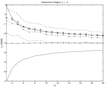
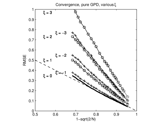
Although there is as yet no proof of consistency for any elemental combination, numerical evidence suggests that the “linearly-rising” combination is consistent for samples drawn from within the GPD family. Fig. 7 shows how the Root Mean Square Error (RMSE) for the “linearly-rising” combination of elementals decreases as the sample size grows. At each point on each graph, the RSME was determined numerically from 10,000 samples of size $N$ drawn from a GPD at various $\xi$ in the range $-3\leq\xi\leq 3$, with $N$ increasing from 20 to 1000. At each $\xi$, and for $N$ large, the errors appear to be converging with increasing sample size $N$ at a rate proportional to $1/\sqrt{N}$, with the constant of proportionality dependent on $\xi$.

There is a consistency proof already in existence which has some relevance here, and covers many elemental combinations for the more general domain of attraction case (which trivially includes the pure GPD case). This is Theorem 3.1 of Segers (2005), which guarantees weak consistency of many elemental combinations in the $N\rightarrow\infty$, $k\rightarrow\infty$, $k/N\rightarrow 0$ limit. To be covered by this theorem, elemental combinations must be expressible as a mixture of Segers estimators satisfying a condition (Condition 2.5, Segers (2005)), which re-stated in the notation here, requires the log-spacing weight matrix $A$ to have zero weights in the vicinity of the diagonal and of the top row. The linearly-rising combination does not satisfy this condition, although it is clear that minor adjustments can be made to zero the weights in the appropriate vicinities.

Finally, it could be noted that the presence (or lack) of asymptotic consistency results is arguably of limited interest if the emphasis, as here, is on providing estimators which perform well with small or moderately sized samples.

Figure 7: Dependence of root mean square error RMSE on sample size $N$ ($20\leq N\leq 1000$) for the linearly-rising combination, with samples drawn from GPDs with various tail parameters. Positive and negative $\xi$ are indicated with circles and crosses respectively. Horizontal axes are scaled to bring infinite $N$ to unity, by plotting $1-\sqrt{2/N}$. This numerical evidence suggests that, for large $N$, the RMSE decreases in proportion to $1/\sqrt{N}$, with the constant of proportionality depending on $\xi$.

7 Summary

‘Elemental’ absolutely-unbiased, location- and scale-invariant estimators for the tail parameter $\xi$ of the GPD have been presented, valid for all $\xi$ and all $N\geq 3$. The elemental estimators were shown to form a complete basis for those unbiased, location and scale-invariant estimators of the GPD tail parameter which are constructed from linear combinations of log-spacings. Numerical evidence was presented which supports consistency of at least one elemental combination for samples drawn from the pure GPD family.

Appendix 1: Proof that $\log\tau^{J-1}/t^{I}$ is unbiased for the GPD

Consider a random variable $x$ with distribution function $F(x)$ and complement $G(x)=1-F(x)$, and via the probability integral transform, construct the inverse function $x=u(G)$ which maps an exceedence probability $G$ to a point $x$ in the data space. Since $dG=-dF/dx\ dx=-p(x)\ dx$ where $p(x)$ is the density, the expected value of any function $h(x)$ may be evaluated by transforming integrals over $x$ to integrals over $G$, using :

$$\langle h(x)\rangle=\int_{\forall x}h(x)\ p(x)\ dx=\int_{0}^{1}h(u(G))\ dG$$ (3)

A consequence of the well-known uniform density of the $G$’s is that the second integral (over $G$) can be considerably simpler than the first integral (over $x$). For the GPD, integrals via $p(x)$ lead to lengthy expressions involving hypergeometric (Lauricella) functions. Although a proof that the elemental estimators are unbiased has been constructed by that route, the approach via the transformed integrals over $G$ is considerably simpler, and is presented here.

Consider an ordered sample $\bm{X}$ of $n$ data points drawn from the distribution $F$, ordered such that $X_{n}\leq X_{n-1}\leq\ldots\leq X_{2}\leq X_{1}$. The expected value of any function $h(\bm{X})$ is

$$\langle h(\bm{X})\rangle=n!\ \int_{0}^{1}dG_{n}\ldots\int_{0}^{G_{2}}dG_{1}\ h(u(\bm{G}))$$ (4)

the integral being over the $n$-dimensional unit simplex containing all possible $G$.

$$\text{The GPD has distribution function}\ F(x) = 1-\left(1+\frac{\xi(x-\mu)}{\sigma}\right)^{-1/\xi}$$ (5)

$$\text{such that}\ x = u(G)=\mu+\frac{\sigma}{\xi}(G^{-\xi}-1)$$ (6)

Depending whether $\xi$ is positive or negative, the expected value of the log-spacing between the $i$th and $j$th order statistics is

$$\langle\log(X_{i}-X_{j})\rangle=\begin{cases}\langle\log(G_{j}^{\gamma}-G_{i}^{\gamma})\rangle-\gamma\langle\log G_{i}G_{j}\rangle+\log\frac{\sigma}{\gamma}&\text{for}\ \xi=\gamma,\ \ \gamma>0\\ \langle\log(G_{j}^{\gamma}-G_{i}^{\gamma})\rangle\hskip 59.75095pt+\log\frac{\sigma}{\gamma}&\text{for}\ \xi=-\gamma,\ \gamma>0\end{cases}$$ (7)

Consider an estimator $\ \hat{\xi}(\bm{X})=\sum_{i,j}a_{ij}\log(X_{i}-X_{j})$, a linear combination of log-spacings. For $\hat{\xi}$ to be scale invariant, the weights $a_{ij}$ must sum to zero to remove the $\sigma$ dependence in Eqn. (7). Moreover, for $\hat{\xi}$ to be unbiased for both positive and negative $\xi$, Eqn. (7) requires

$$\sum_{i,j}a_{ij}\langle\log(G_{j}^{\gamma}-G_{i}^{\gamma})\rangle=-\gamma\ \ \ \text{and}\ \ \ -\sum_{i,j}a_{ij}\gamma\langle\log G_{i}G_{j}\rangle=2\gamma$$ (8)

To determine the expected value of any function $h(X_{i},X_{j})$, all other $G$ variables can be integrated out, leaving

$$\langle h(X_{i},X_{j})\rangle=C_{ij}\int_{0}^{1}\ dG_{j}\int_{0}^{G_{j}}dG_{i}\ \ \ G_{i}^{i-1}(1-G_{j})^{n-j}(G_{j}-G_{i})^{j-i-1}\ h(u(G_{i}),u(G_{j}))$$ (9)

where $C_{ij}=n!/((i-1)!(n-j)!(j-i-1)!)$. For example

$$\sum a_{ij}\langle\log G_{j}\rangle=\sum a_{ij}C_{ij}.\int_{0}^{1}G_{j}^{j-1}(1-G_{j})^{n-j}\log G_{j}\ dG_{j}\ .\ \int_{0}^{1}\phi^{i-1}(1-\phi)^{j-i-1}\ d\phi$$ (10)

where $\phi=G_{i}/G_{j}$. The $\phi$ integral leads immediately to the beta function $B(i,j-i)$. For the $G_{j}$ integral, standard Mellin transform theory gives

$$\int_{0}^{1}G_{j}^{j-1}(1-G_{j})^{n-j}\log G_{j}\ dG_{j} = \left[\frac{d}{ds}\int_{0}^{1}G_{j}^{s-1+j-1}(1-G_{j})^{n-j}\ dG_{j}\right]_{s=1}$$ (11)

$$= B(j,n-j+1)\left(\psi(j)-\psi(n+1)\right)$$

where $\psi$ is the digamma function, the derivative of the logarithm of the gamma function. Both beta functions have integer arguments and may be expressed as ratios of factorials. These cancel with the leading factorial terms $C_{ij}$, such that the expected value of the weighted sum is

$$\sum a_{ij}\langle\log G_{j}\rangle=\sum a_{ij}\left(\psi(j)-\psi(n+1)\right)=\sum a_{ij}\psi(j)$$ (12)

the last step following from $\sum a_{ij}=0$. It follows similarly that

$$\sum a_{ij}\langle\log G_{i}\rangle=\sum a_{ij}\left(\psi(i)-\psi(n+1)\right)=\sum a_{ij}\psi(i)$$ (13)

For an individual elemental $\hat{\xi}_{IJ}$ the weights $a_{ij}$ and the relevant values of $i$ and $j$ are given in Table 3.

Table 3: The indices of an elemental estimator, and, in the final column, the weights.

term	$i$	$j$	$a_{ij}$
$\log{(X_{I}-X_{J-1})}$	$I$	$J-1$	$J-1$
$\log{(X_{I}-X_{J})}$	$I$	$J$	$-(J-I-1)$
$\log{(X_{I+1}-X_{J})}$	$I+1$	$J$	$-I$

Using the relation $\psi(1+x)=\psi(x)+1/x$ we obtain the contributions from the individual elemental $\hat{\xi}_{IJ}$ to be

$$\sum a_{ij}\psi(j) = (J-1)\psi(J-1)-(J-I-1)\psi(J)-I\psi(J)$$ (14)

$$= (J-1)(\psi(J-1)-\psi(J))=-1$$

$$\sum a_{ij}\psi(i) = (J-1)\psi(I)-(J-I-1)\psi(I)-I\psi(I+1)$$ (15)

$$= \ I(\psi(I)-\psi(I+1))\ =\ -1$$

These are exactly what is required to show that any unit-sum linear combination $\hat{\xi}$ of elementals provides an unbiased estimate for $\xi$ via the $\langle\log G_{i}^{\gamma}\rangle$ and $\langle\log G_{j}^{\gamma}\rangle$ terms. Explicitly, with $\gamma=|\xi|$, we have

$$\langle\hat{\xi}\rangle = \left\{\begin{array}[]{ll}\ \gamma\sum a_{ij}\langle\log G_{j}\rangle+\sum a_{ij}\langle\log(1-\phi^{\gamma})\rangle&\mbox{for $\xi<0$ }\\ -\gamma\sum a_{ij}\langle\log G_{i}\rangle+\sum a_{ij}\langle\log(1-\phi^{\gamma})\rangle&\mbox{for $\xi>0$ }\end{array}\right.$$ (18)

$$= \xi+\sum a_{ij}\langle\log(1-\phi^{\gamma})\rangle\ \ \$$ (19)

It only remains to prove that the second term is zero. This term involves somewhat more complicated integrals leading to sums of digamma functions with non-integer arguments dependent on $\gamma$. Explicit evaluation of these can, however, be avoided here by observing how the elemental terms combine and cancel.

From Eqn. (9), we obtain

$$\langle\log(1-\phi_{ij}^{\gamma})\rangle = C_{ij}D_{j}B_{ij}$$

$$\text{where}\ \ D_{j} = \int_{0}^{1}y^{j-1}(1-y)^{n-j}\ dy=\frac{(j-1)!(n-j)!}{n!}$$

$$\text{and}\ \ \ B_{ij} = \int_{0}^{1}\phi^{i-1}(1-\phi)^{j-i-1}\log(1-\phi^{\gamma})\ d\phi$$ (20)

Summing over a single elemental using the weights $a_{ij}$ given in Table 3, and collecting the leading $a_{ij}C_{ij}Dj$ terms gives

$$\sum a_{ij}\langle\log(1-\phi^{\gamma})\rangle=\frac{(J-1)!}{(I-1)!(J-I-2)!}(B_{I,J-1}-B_{I,J}-B_{I+1,J})\\$$ (21)

Now

$$B_{I,J-1}-B_{I,J}-B_{I+1,J}=$$

$$\int_{0}^{1}\{\phi^{I-1}(1-\phi)^{J-I-2}-\phi^{I-1}(1-\phi)^{J-I-1}-\phi^{I}(1-\phi)^{J-I-2}\}\log(1-\phi^{\gamma})\ d\phi$$

where the integrand contains the factor $\left[1-(1-\phi)-\phi\right]=0$, thus

$$\sum a_{ij}\langle\log(1-\phi^{\gamma})\rangle=0\ \ \ \ \ \ \ \forall\xi\neq 0$$ (23)

This completes the proof for all nonzero $\xi$.

The proof for $\xi=0$ follows similarly, using $G(x)=\exp{(-(x-\mu)/\sigma)}$, whence, using Eqn. (9), we obtain

$$\sum a_{ij}\langle\log(X_{i}-X_{j})\rangle=\sum a_{ij}\langle\log\sigma\rangle+\sum a_{ij}\langle\log[-\log\phi_{ij}]\rangle$$ (24)

The first term is trivially zero due to the zero sum of the elemental $a_{ij}$, and the second term is zero for the same reason that $\sum a_{ij}\langle\log(1-\phi^{\gamma})\rangle$ is zero, as shown above, in that the elementals combine terms in such a way as to eliminate the expectation of any function of the $\phi_{ij}$.

This completes the proof that for any elemental $\hat{\xi_{IJ}}$ , the expectation $\langle\hat{\xi_{IJ}}\rangle=\xi$ for all $\xi$.

Appendix 2: Completeness

Here we prove that for an estimator $\hat{\xi}$ of the tail parameter $\xi$ of the GPD, with the preconditions that $\hat{\xi}$ is i) a linear combination of log-spacings, ii) absolutely-unbiased for all $\xi$ and iii) location- and scale-invariant, then $\hat{\xi}$ may be expressed as a linear combination of the elementals. That is, the elementals form a complete basis for the set of invariant unbiased log-spacing estimators of the GPD tail parameter.

Precondition ii requires that $\hat{\xi}$ must be unbiased at both $\xi=\gamma$ and $\xi=-\gamma$ for any $\gamma>0$. This symmetry is embodied in Eqn. (7), addition and subtraction of which (together with precondition iii and elementary integrations such as Eqns 10-12) leads to the requirements on the log-spacing weights $a_{ij}$ that

$$\gamma\sum a_{ij}(\langle\log G_{j}\rangle+\langle\log G_{i}\rangle)$$ (25)

$$= \gamma\sum a_{ij}\left[\psi(j)+\psi(i)\right]=-2\gamma$$

$$\gamma\sum a_{ij}(\langle\log G_{j}\rangle-\langle\log G_{i}\rangle)$$ (26)

$$= \gamma\sum a_{ij}\left[\psi(j)-\psi(i)\right]=-2\sum a_{ij}\langle\log(1-\phi_{ij}^{\gamma})\rangle$$

where $\psi$ is the digamma function and $\sum$ means sum over $i$ from 1 to $N-1$ and $j$ from $i+1$ to $N$.
We now prove that the preconditions imply that the right-hand side of Eqn (26) is zero. Eqn (26) may be written as

$$c_{1}\gamma=\sum a_{ij}\langle\log(1-\phi_{ij}^{\gamma})\rangle:=I_{1}\ \text{ where }c_{1}=-(1/2)\sum a_{ij}\left[\psi(j)-\psi(i)\right]$$ (27)

Similar to Eqn (10), each term in the $I_{1}$ summation may be considered individually and all variables irrelevant to that term may be integrated out to give

$$I_{1}=\sum_{ij}a_{ij}C_{ij}\int_{0}^{1}G_{j}^{j-1}(1-G_{j})^{n-j}\ dG_{j}\ .\ \int_{0}^{1}{\phi_{ij}}^{i-1}(1-\phi_{ij})^{j-i-1}\log(1-\phi_{ij}^{\gamma})\ d\phi_{ij}$$ (28)

The $G_{j}$ integral gives a beta function $B(j,n-j+1)$ which combines with the $C_{ij}$ term to give a factor $1/B(i,j-i)$. Since each expectation integral over $\phi_{ij}$ is definite, we can set each $\phi_{ij}=\phi$. Each product $\phi^{i-1}(1-\phi)^{j-i-1}$ involves integer exponents and can thus be expressed as a polynomial of degree $j-2$. Passing the summation through the integral sign, the various polynomials can be collected into a single polynomial $p_{n-2}(\phi)=\sum_{k=0}^{n-2}b_{k}\phi^{k}$ of degree $n-2$. Passing the summation back out of the integral gives:

$$I_{1}=\sum_{k=0}^{n-2}b_{k}g_{k}(\gamma)\ \text{ where }\ g_{k}(\gamma):=\int_{0}^{1}\phi^{k}\log(1-\phi^{\gamma})\ d\phi$$ (29)

The binomial expansion of each $(1-\phi)^{j-i-1}$ factor in Eqn. 28 leads to the total polynomial

$$p_{n-2}(\phi)=\sum_{i=1}^{n-1}\sum_{j=i+1}^{n}\frac{(j-1)!}{(i-1)!(j-i-1)!}a_{ij}\sum_{q=0}^{j-i-1}\frac{(-1)^{q}(j-i-1)!}{q!(j-i-1-q)!}\phi^{(i-1)+q}$$ (30)

Collecting together equal powers of $\phi$ gives

$$p_{n-2}(\phi)=\sum_{k=0}^{n-2}\phi^{k}\sum_{i=1}^{k+1}\sum_{j=k+2}^{n}\frac{(j-1)!}{(i-1)!}a_{ij}\frac{(-1)^{k-i-1}}{(k-i+1)!(j-k-2)!}$$ (31)

such that the polynomial coefficients $b_{k}$ are

$$b_{k} = \sum_{i=1}^{k+1}\sum_{j=k+2}^{n}\frac{(j-1)!}{(i-1)!}a_{ij}\frac{(-1)^{k-i-1}}{(k-i+1)!(j-k-2)!}$$ (36)

$$= (k+1)\sum_{j=k+2}^{n}\left(\begin{array}[]{c}j-1\\ k+1\end{array}\right)\sum_{i=1}^{k+1}\left(\begin{array}[]{c}k\\ i-1\end{array}\right)(-1)^{k-i-1}a_{ij}$$

Having determined the polynomial coefficients, we consider the integrals $g_{k}(\gamma)$ of the various $\phi^{k}$ terms, as defined in Equation (29). The transformation $\phi^{\gamma}=(1-\rho)$ leads to

$$g_{k}(\gamma) = \frac{1}{\gamma}\int_{0}^{1}(1-\rho)^{\frac{k+1}{\gamma}-1}\log\rho\ d\rho=\frac{1}{\gamma}\left[\frac{d\ }{ds}\int_{0}^{1}\rho^{s-1}(1-\rho)^{\frac{k+1}{\gamma}-1}\ d\rho\right]_{s=1}$$ (37)

$$= \frac{1}{\gamma}B(1,\frac{k+1}{\gamma})\left[\psi(1)-\psi(1+\frac{k+1}{\gamma})\right]$$

$$= \frac{1}{k+1}\left[\psi(1)-\psi(1+\frac{k+1}{\gamma})\right]$$

We thus have

$$I_{1}=c_{1}\gamma=\sum_{k=0}^{n-2}b_{k}.g_{k}(\gamma)=\sum_{k=0}^{n-2}\frac{b_{k}}{k+1}\left[\psi(1)-\psi(1+\frac{k+1}{\gamma})\right]$$ (38)

If this is true at all $\gamma>0$, then it must be true for $\gamma$ large, ($\gamma=1/\epsilon$, $\epsilon>0$, $\epsilon$ small). There

$$g_{k}\left(\gamma=\frac{1}{\epsilon}\right)=\frac{1}{k+1}\left[\psi(1)-\psi(1+(k+1)\epsilon)\right]$$

Since the digamma function is well-behaved (i.e. infinitely differentiable) near $\psi(1)$, we may take the Taylor series $\psi(1+\delta)=\psi(1)+\psi^{\prime}(1)\delta+O(\delta^{2})$ to obtain

$$g_{k}(\gamma)=-\psi^{\prime}(1)\epsilon+O(\epsilon^{2})$$ (39)

thus

$$I_{1}=c_{1}\gamma=\frac{c_{1}}{\epsilon}=\sum_{k=0}^{n-2}b_{k}g_{k}(\frac{1}{\epsilon})=-\epsilon\psi^{\prime}(1)\sum_{k=0}^{n-2}{b_{k}}+O(\epsilon^{2})$$ (40)

whence

$$c_{1}=-\epsilon^{2}\psi^{\prime}(1)\sum_{k=0}^{n-2}{b_{k}}+O(\epsilon^{3})$$ (41)

Since $c_{1}$ is a constant wrt $\gamma$ and since (nonzero) $\epsilon=1/\gamma$ can be arbitrarily small, we thus infer from 41 that the preconditions imply that $c_{1}=0$.

Finally, since the preconditions imply that $I_{1}=c_{1}\gamma=0$ and $I_{1}=\sum_{k=0}^{n-2}b_{k}\ g_{k}(\gamma)$ the independence of the $N-1$ functions $g_{k}(\gamma)$ implies that

$$b_{k}=0,\ \ \forall k\in\{0,1,\ldots,n-2\}$$ (42)

These are the $N-1$ constraints needed to reduce the dimension of the problem down to that spanned by the elementals.

That the elementals are contained within this subspace can be readily checked by gathering, within each $b_{k}$ summation, the terms associated with each elemental crosshair of the grid $G$. Each $b_{k}=0$ constraint corresponds to a weighted summation over a subrectangle of the $A$ matrix as illustrated in Table 4.

.	$a_{12}$	$a_{13}$	$a_{14}$	$a_{15}$	$a_{16}$	$a_{17}$
		$a_{23}$	$a_{24}$	$a_{25}$	$a_{26}$	$a_{27}$
			$a_{34}$	$a_{35}$	$a_{36}$	$a_{37}$
				$a_{45}$	$a_{46}$	$a_{47}$
					$a_{56}$	$a_{57}$
						$a_{67}$

Table 4: Each constraint $b_{k}=0$ is a summation over a rectangle of the $A$ matrix. For $N=7$, the rectangle of terms for $k=3$ is shown.

Consider an element $a_{IJ}$ away from the rectangle boundaries (such as $a_{26}$ in Table 4). Consider the $b_{k}$ summation terms associated with the elemental $\hat{\xi}_{IJ}$, which thus involves the term $a_{IJ}$, the term $a_{I,J-1}$ to its left and the term $a_{I+1,J}$ below it. The $b_{k}$ summation weights given to each of these terms can be obtained from Eqn 36 as

$$b_{k,(I,J)} = \frac{(J-1)!(+1)}{(I-1)!(k-I+1)!(J-k-2)!}$$ (43)

$$b_{k,(I,J-1)} = \frac{(J-2)!(+1)}{(I-1)!(k-I+1)!(J-k-3)!}$$ (44)

$$\text{and}\ b_{k,(I+1,J)} = \frac{(J-1)!(-1)}{(I)!(k-I)!(J-k-2)!}$$ (45)

The elemental $\hat{\xi}_{IJ}$ contributes in proportions $-(J-I-1)$, $(J-1)$ and $-I$ to $a_{IJ}$, $a_{I,J-1}$ and $a_{I+1,J}$ respectively. The weights in the $b_{k}$ summation are thus such as to eliminate the contribution from the elemental $\xi_{IJ}$, since it readily follows from the above that

$$-(J-I-1)b_{k,(I,J)}+(J-1)b_{k,(I,J-1)}+(-I)b_{k,(I+1,J)}$$

$$\propto -(J-I-1)+(k-I+1)+(J-k-2)$$

$$= 0$$ (47)

(The proof for elements near the boundaries of the $b_{k}$ rectangle is similar).

Since any elemental satisfies the constraints then so does any linear combination thereof, and since there are $(N-1)(N-2)/2$ elementals and they are independent, it follows that they form a complete basis for those estimators of the GPD tail index that satisfy the preconditions given.

References

- Castillo and Daoudi (2009) Castillo, J., Daoudi, J., 2009. Estimation of the generalized Pareto distribution. Statistics and Probability Letters 79, 684–688.
- Coles (2001) Coles, S., 2001. An Introduction to Statistical Modelling of Extreme Values. Springer, London.
- de Zea Bermudez and Kotz (2010) de Zea Bermudez, P., Kotz, S., 2010. Parameter estimation for the generalized Pareto distribution - parts i and ii. J. Stat. Planning and Inference 140 (6), 1353–1388.
- Dekkers et al. (1989) Dekkers, A. L. M., Einmahl, J. H. J., deHaan, L., 1989. A moment estimator for the index of an extreme value distribution. Annals of Statistics 17, 1833–1855.
- Drees (1998) Drees, H., 1998. A general class of estimators of the extreme value index. J. Stat. Planning and Inference 66, 95–112.
- Embrechts et al. (1999) Embrechts, P., Klüppelberg, C., Mikosch, T., 1999. Modelling Extreme Events for Insurance and Finance. Springer, Berlin.
- Hill (1975) Hill, B. M., 1975. A simple general approach to inference about the tail of a distribution. Annals of Statistics 3, 1163–1174.
- Hosking and Wallis (1987) Hosking, J. R. M., Wallis, J. R., 1987. Parameter and quantile estimation for the Generalized Pareto Distribution. Technometrics 29 (3), 339–349.
- Pickands (1975) Pickands, J., 1975. Statistical inference using extreme order statistics. Ann. Statist. 3, 119–131.
- Reiss and Thomas (2001) Reiss, R.-D., Thomas, M., 2001. Statistical Analysis of Extreme Values: with applications to insurance, finance, hydrology and other fields. Birkhäuser, Basel.
- Segers (2005) Segers, J., 2005. Generalized Pickands estimators for the extreme value index. J. Stat. Planning and Inference 128 (2), 381–396.
- Smith (1987) Smith, R. L., 1987. Estimating tails of probability distributions. Annals of Statistics 15 (3), 1174–1207.
- Yun (2002) Yun, S., 2002. On a generalized Pickands estimator of the extreme value index. J. Stat. Planning and Inference 102, 389–409.
Appendix 1: Proof that is unbiased for the GPD
Consider a random variable with distribution function and complement , and via the probability integral transform, construct the inverse function which maps an exceedence probability to a point in the data space. Since where is the density, the expected value of any function may be evaluated by transforming integrals over to integrals over , using :