RGE of a Cold Dark Matter Two-Singlet Model

Abstract

We study via the renormalization group equations at one-loop order the perturbativity and vacuum stability of a two-singlet model of cold dark matter (DM) that consists in extending the Standard Model with two real gauge-singlet scalar fields. We then investigate the regions in the parameter space in which the model is viable. For this, we require the model to reproduce the observed DM relic density abundance, to comply with the measured XENON 100 direct-detection upper bounds, and to be consistent with the RGE perturbativity and vacuum-stability criteria up to $40\mathrm{TeV}$. For small mixing angle $\theta$ between the physical Higgs $h$ and auxiliary field, and DM-$h$ mutual coupling constant $\lambda_{0}^{\left(4\right)}$, we find that the auxiliary-field mass is confined to the interval $116\mathrm{GeV}-138\mathrm{GeV}$ while the DM mass is mainly confined to the region above $57\mathrm{GeV}$. Increasing $\theta$ enriches the existing viability regions without relocating them, while increasing $\lambda_{0}^{\left(4\right)}$ shrinks them with a tiny relocation. We show that the model is consistent with the recent Higgs boson-like discovery by the ATLAS and CMS experiments, while very light dark matter (masses below $5\mathrm{GeV}$) is ruled out by the same experiments.

I Introduction

Now that there is more and more compelling evidence that the discovery in the ATLAS and CMS experiments at the LHC is a Higgs particle with a mass $m_{h}\simeq 125\mathrm{GeV}$ ATLAS ; CMS , one of the main focuses of particle physics is an understanding of the still elusive nature of dark matter (DM), believed to account for about 26% of the energy content of the universe dm-observation . Side by side with observation, models beyond the Standard Model (SM) are devised to account for weakly interacting massive particles (WIMPs) as plausible candidates for dark matter. Such models range from the sophisticated ones, those bearing intricate underlying symmetries and mechanisms of symmetry breaking, to the more simpler ones, those extending the SM without any particular assumption regarding a deeper structure.

Since the findings at the LHC have so far yielded no particular clue as to possible particle structures beyond those of the Standard Model, it is therefore still consistent to try to recognize dark matter as simple WIMPs extending the Standard Model, with no further assumptions as to inner structures. The simplest of such extensions is a one real electroweak-singlet scalar field, interacting with visible matter only via the SM Higgs particle, first proposed by Silveira and Zee SZ and further studied in MD ; BP ; one-singlet . In this minimal model, with DM masses lighter than $10\mathrm{GeV}$, the Higgs would be mainly invisible, which is excluded by the recent measurement of the Higgs signal at the LHC Hinv . Also, for DM masses in the range $7\mathrm{GeV}-60\mathrm{GeV}$, the model is ruled out by the data from XENON 10 XENON10 and CDMS II CDMSII , except around the resonance $62\mathrm{GeV}$ at which the Higgs-DM coupling is extremely small. Furthermore, DM masses between $65\mathrm{GeV}$ and $80\mathrm{GeV}$ are excluded in this one-singlet extension by the XENON 100 experiment XENON100 . Note that similar conclusions hold also for a complex scalar singlet extension of the SM complex .

So, given the difficulties this minimal model has with existing experimental and observational DM data one-singlet-difficulties , we have proposed in abada-ghaffor-nasri an extension to the Standard Model with two real electroweak singlets, one being stable, the DM candidate, and the other an auxiliary field with a spontaneously broken $\mathbb{Z}_{2}$ symmetry. Based on the DM relic-density and WIMP direct detection studies, we have concluded that this two-singlet model is capable of bearing dark matter in a large region of the parameter space. Further constraints on the model as well as some of its phenomenological implications have been studied in abada-nasri-1 where rare meson decays and Higgs production channels have been considered.

In the present work, we further the study of the two-singlet model and ask how high in the energy scale it is computationally reliable. A standard treatment is the investigation of the running of the coupling constants in terms of the mass scale $\Lambda$ via the renorrmalization group equations (RGE). We believe one-loop calculations are amply sufficient for the present task; higher loops could be considered if the situation changes.

The two standard issues to monitor are the perturbativity of the scalar coupling constants and the vacuum stability of the theory. These issues were studied in GLR for the complex scalar singlet extension of the SM, and it was shown that the vacuum-stability requirement can affect the DM relic density. Specific results from such studies depend on the cutoff scale $\Lambda_{m}$ of the theory. Reversely, imposing perturbativity and vacuum stability may indicate at what $\Lambda_{m}$ the two-singlet extension is valid. In the early parts of this work, the second point of view is adopted, whereas in the later part, the first is taken. Furthermore, up to only recently, it has been anticipated that new physics such as supersymmetry would appear at the LHC at the scale $\Lambda\sim 1\mathrm{TeV}$. Present results from ATLAS and CMS indicate no such signs yet. One consequence of this is that the cutoff scale $\Lambda_{m}$ may be higher. As we shall discuss, we find that it can be $\sim 40\mathrm{TeV}$.

This work is organized as follows. After this introduction, we recapitulate in section II the essentials of the two-singlet model necessary for the RGE calculations. In section III, we discuss the running of the scalar coupling constants when we switch off the non-Higgs SM particles. This gives us a first understanding of how high in the energy scale perturbativity is allowed. It helps also seeing the subsequent effects of the other SM particles. Section IV discusses the full RGEs. Vacuum stability gets into focus with the Higgs coupling constant turning negative at some scale. The mass scales at which non-perturbativity and non-stability set in are different, and so a choice for $\Lambda_{m}$ has to be made. Section V attempts at finding the regions in the parameter space in which the model is predictive. In addition to the DM relic-density constraint and the perturbativity-stability criteria deduced from the previous two sections, we impose on the model to be within the current direct-detection experimental bounds. Section VI is devoted to concluding remarks.

II The two-singlet model

The model is obtained by adding to the Standard Model two real, spinless, and $\mathbb{Z}_{2}$-symmetric SM-gauge-singlet fields. One is the dark matter field $S_{0}$ with unbroken $\mathbb{Z}_{2}$ symmetry, and the other an auxiliary field $\chi_{1}$ with spontaneously broken $\mathbb{Z}_{2}$ symmetry. Both fields interact with the SM particles via the Higgs doublet $H$. Using the same notation as in abada-ghaffor-nasri , the potential function that involves $S_{0}$, $H$ and $\chi_{1}$ is:

$$U = \frac{\tilde{m}_{0}^{2}}{2}S_{0}^{2}-\mu^{2}H^{\dagger}H-\frac{\mu_{1}^{2}}{2}\chi_{1}^{2}$$ (1)

$$+\frac{\eta_{0}}{24}S_{0}^{4}+\frac{\lambda}{6}\left(H^{\dagger}H\right)^{2}+\frac{\eta_{1}}{24}\chi_{1}^{4}+\frac{\lambda_{0}}{2}S_{0}^{2}H^{\dagger}H+\frac{\eta_{01}}{4}S_{0}^{2}\chi_{1}^{2}+\frac{\lambda_{1}}{2}H^{\dagger}H\chi_{1}^{2},$$

where $\tilde{m}_{0}^{2}$, $\mu^{2}$and $\mu_{1}^{2}$ and all the coupling constants are real positive numbers.

We are interested in monitoring the running of the scalar coupling constants. A one-loop renormalization-group calculation yields the following $\beta$-functions:

$$\beta_{\eta_{0}} = \frac{3}{16\pi^{2}}\left(\eta_{0}^{2}+\eta_{01}^{2}+4\lambda_{0}^{2}\right);$$

$$\beta_{\eta_{1}} = \frac{3}{16\pi^{2}}\left(\eta_{1}^{2}+\eta_{01}^{2}+4\lambda_{1}^{2}\right);$$

$$\beta_{\lambda} = \frac{3}{16\pi^{2}}\left(\frac{4}{3}\lambda^{2}+\lambda_{0}^{2}+\lambda_{1}^{2}-48\lambda_{t}^{4}+8\lambda\lambda_{t}^{2}-3\lambda g^{2}-\lambda g^{\prime}{}^{2}+\frac{3}{2}g^{2}g^{\prime}{}^{2}+\frac{9}{4}g^{4}\right);$$

$$\beta_{\eta_{01}} = \frac{1}{16\pi^{2}}\left(4\eta_{01}^{2}+\eta_{0}\eta_{01}+\eta_{1}\eta_{01}+4\lambda_{0}\lambda_{1}\right);$$

$$\beta_{\lambda_{0}} = \frac{1}{16\pi^{2}}\left(4\lambda_{0}^{2}+\lambda_{0}\eta_{0}+2\lambda_{0}\lambda+\eta_{01}\lambda_{1}+12\lambda_{0}\lambda_{t}^{2}-\frac{9}{2}\lambda_{0}g^{2}-\frac{3}{2}\lambda_{0}g^{\prime}{}^{2}\right);$$

$$\beta_{\lambda_{1}} = \frac{1}{16\pi^{2}}\left(4\lambda_{1}^{2}+\lambda_{1}\eta_{1}+2\lambda_{1}\lambda+\eta_{01}\lambda_{0}+12\lambda_{1}\lambda_{t}^{2}-\frac{9}{2}\lambda_{1}g^{2}-\frac{3}{2}\lambda_{1}g^{\prime}{}^{2}\right).$$ (2)

As usual, $\beta_{g}\equiv dg/d\ln\Lambda$ where $\Lambda$ is the running mass scale, starting from $\Lambda_{0}=100\mathrm{GeV}$. The constants $g$, $g^{\prime}$ and $g_{s}$ are the SM and strong gauge couplings, known SM-results and given to one-loop order by the expression:

$$G\left(\Lambda\right)=\frac{G\left(\Lambda_{0}\right)}{\sqrt{1-2a_{G}\,G^{2}\left(\Lambda_{0}\right)\,\ln\left(\frac{\Lambda}{\Lambda_{0}}\right)}},$$ (3)

where $a_{G}=\frac{-19}{96\pi^{2}},\frac{41}{96\pi^{2}},\frac{-7}{16\pi^{2}}$, and $G\left(\Lambda_{0}\right)=0.65$, $0.36,1.2$ for $G=g,g^{\prime},g_{s}$ respectively. The coupling constant $\lambda_{t}$ is that between the Higgs field and the top quark. To one-loop order, it runs according to SM-results :

$$\beta_{\lambda_{t}}=\frac{\lambda_{t}}{16\pi^{2}}\left(9\lambda_{t}^{2}-8g_{s}^{2}-\frac{9}{4}g^{2}-\frac{17}{12}g^{\prime 2}\right),$$ (4)

with $\lambda_{t}\left(\Lambda_{0}\right)=\frac{m_{t}\left(\Lambda_{0}\right)}{v}=0.7$, where $v$ is the Higgs vacuum expectation value (vev) and $m_{t}$ the top mass. Note that we are taking into consideration the fact that the top-quark contribution is dominant over that of the other fermions of the Standard Model.

The model undergoes two spontaneous breakings of symmetry: one of the electroweak, with a vev $v=246~{}\mathrm{GeV}$, and one of the $\mathbb{Z}_{2}$ symmetry ($\chi_{1}$ field), with a vev $v_{1}$ we take in this work equal to $150~{}\mathrm{GeV}$. Above $v$, the fields and parameters of the theory are those of (1). Below $v_{1}$, the (scalar) physical fields are $S_{0}$ (DM), $h$ (Higgs) and $S_{1}$ (auxiliary), with parameters (masses and coupling constants) given in Eqs. (2.2–2.15) of abada-ghaffor-nasri . We take the values of the physical parameters at the mass scale $\Lambda_{0}=100~{}\mathrm{GeV}$. There are originally nine free physical parameters. The two vevs $v$ and $v_{1}$ are fixed, as well as the mass of the physical Higgs field $m_{h}=125~{}\mathrm{GeV}$ ATLAS ; CMS . Also, the physical mutual coupling constant $\eta_{01}^{(4)}$ between $S_{0}$ and $S_{1}$ is determined by the DM relic-density constraint Planck , which translates into the condition:

$$\left\langle v_{12}\sigma_{\mathrm{ann}}\right\rangle\simeq 1.7\times 10^{-9}\,\mathrm{GeV}^{-2},$$ (5)

where $\left\langle v_{12}\sigma_{\mathrm{ann}}\right\rangle$ is the thermally averaged annihilation cross-section of a pair of two DM particles times their relative speed in the center-of-mass reference frame. This constraint is imposed throughout this work, together with the perturbativity restriction $0\leq\eta_{01}^{(4)}\leq\sqrt{4\pi}$ on its solution. The remaining free parameters of the model are the physical mutual coupling constant $\lambda_{0}^{(4)}$ between $h$ and $S_{0}$, the mixing angle $\theta$ between $h$ and $S_{1}$, the DM mass $m_{0}$, the mass $m_{1}$ of the auxiliary physical field $S_{1}$, and the DM self-coupling constant $\eta_{0}$. This latter has so far been decoupled from the other coupling constants abada-ghaffor-nasri ; abada-nasri-1 , but not anymore in view of (2) now that the running is the focus. However, its initial value $\eta_{0}\left(\Lambda_{0}\right)$ is arbitrary and its $\beta$-function is always positive. This means $\eta_{0}\left(\Lambda\right)$ will only increase as $\Lambda$ increases, quickly if starting from a rather large initial value, slowly if not. Therefore, without loosing generality in the subsequent discussion, we fix $\eta_{0}\left(\Lambda_{0}\right)=1$. Hence, here too we still effectively have four free parameters: $\lambda_{0}^{(4)}$, $\theta$, $m_{0}$, and $m_{1}$. The initial conditions for the coupling constants in (1) in terms of these physical free parameters are as follows:

$$\eta_{1}\left(\Lambda_{0}\right) = \frac{3}{2v_{1}^{2}}\left[m_{1}^{2}+m_{h}^{2}+\left|m_{1}^{2}-m_{h}^{2}\right|\left(\cos\left(2\theta\right)+\frac{v}{2v_{1}}\sin\left(2\theta\right)\right)\right];$$

$$\lambda\left(\Lambda_{0}\right) = \frac{3}{2v^{2}}\left[m_{1}^{2}+m_{h}^{2}-\left|m_{1}^{2}-m_{h}^{2}\right|\left(\cos\left(2\theta\right)-\frac{v_{1}}{2v}\sin\left(2\theta\right)\right)\right];$$

$$\lambda_{1}\left(\Lambda_{0}\right) = \frac{\sin\left(2\theta\right)}{2vv_{1}}\left|m_{1}^{2}-m_{h}^{2}\right|;$$

$$\eta_{01}\left(\Lambda_{0}\right) = \frac{1}{\cos\left(2\theta\right)}\left[\eta_{01}^{(4)}\cos^{2}\theta-\lambda_{0}^{(4)}\sin^{2}\theta\right];$$

$$\lambda_{0}\left(\Lambda_{0}\right) = \frac{1}{\cos\left(2\theta\right)}\left[\lambda_{0}^{(4)}\cos^{2}\theta-\eta_{01}^{(4)}\sin^{2}\theta\right].$$ (6)

Note that normally, as we go down the mass scale, we should seam quantities in steps: at $v$, $v_{1}$, and $\Lambda_{0}$. However, the corrections to (6) are of one-loop order times $\ln\frac{v}{v_{1}}$ or $\ln\frac{v_{1}}{\Lambda_{0}}$, small enough for our present purposes to neglect.

III Scalars Only

To see the effects of the scalar couplings only and how up in the mass scale the model can go, we switch off the non-Higgs SM couplings in (2). The perturbativity constraint we impose on all dimensionless scalar coupling constants is $G\left(\Lambda\right)\leq\sqrt{4\pi}$. Vacuum stability means that $G\left(\Lambda\right)\geq 0$ for the self-coupling constants $\eta_{0},\lambda$, and $\eta_{1}$, and the conditions:

$$-\frac{1}{6}\sqrt{\eta_{0}\lambda}\leq\text{$\lambda_{0}$}\leq\sqrt{4\pi};\qquad-\frac{1}{6}\sqrt{\eta_{0}\text{$\eta_{1}$}}\leq\text{$\eta_{01}$}\leq\sqrt{4\pi};\qquad-\frac{1}{6}\sqrt{\text{$\eta_{1}$}\lambda}\leq\text{$\lambda_{1}$}\leq\sqrt{4\pi}$$ (7)

for the mutual couplings $\lambda_{0},\eta_{01}$, and $\lambda_{1}$. Also, as a start, we let the masses $m_{0}$ and $m_{1}$ vary in the interval $1\mathrm{GeV}-200\mathrm{GeV}$.

Figure 1: The running of the self-couplings (scalars only). The self-coupling $\eta_{1}$ of the auxiliary field $\chi_{1}$ dominates over the Higgs self-coupling $\lambda$.

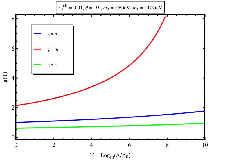
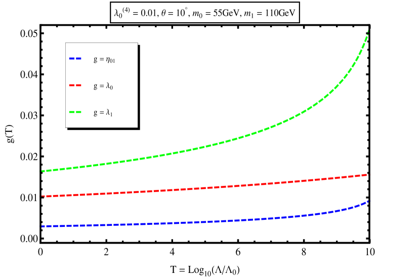
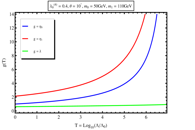
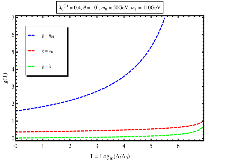
Fig. 1 displays a typical running of the scalar self-coupling constants, from $\Lambda_{0}=10^{2}\mathrm{GeV}$ up to $10^{12}\mathrm{GeV}$. As is expected for scalars only, all coupling constants are increasing functions of the scale $\Lambda$, with different but increasing rates. Also, the larger value the coupling starts from at $\Lambda_{0}$, the faster it will go up. Fig. 2 shows the running of the mutual coupling constants for the same values of the parameters. For these values, the mutual coupling constants start well below 1, and so run low; they are very much dominated by the self-couplings. This situation will stay for $\lambda_{0}$ and $\lambda_{1}$ in all regions, but not for $\eta_{01}$.

The first coupling constant that leaves the perturbativity bound $\sqrt{4\pi}$ is $\eta_{1}$, the self-coupling constant of the auxiliary scalar field $\chi_{1}$, at about $1260~{}\mathrm{TeV}$ for this set of values of the parameters. This behavior is in fact typical. Indeed, $\eta_{1}$ starts above 2 at $\Lambda_{0}$ in all the parameter space, much higher than all the other coupling constants – only $\eta_{01}$ can compete with it in some regions. As it intervenes squared in its own $\beta$-function, it will also move up quicker. More precisely, from (6), we see that $\eta_{1}\left(\Lambda_{0}\right)$ depends on $m_{1}$ and $\theta$ only. The effect of the mixing angle $\theta$ is small. As a function of $m_{1}$, starting from about 2, $\eta_{1}\left(\Lambda_{0}\right)$ decreases slightly until $m_{h}$ and then picks up. It will pass the perturbativity bound $\sqrt{4\pi}$ at about $m_{1}\simeq 160\mathrm{GeV}$. This means that the region $m_{1}>160\mathrm{GeV}$ is automatically excluded from the outset. In actual situations, given the positive-slope RG running of $\eta_{1}\left(\Lambda\right)$ and even in the case of the full RGE (see below), perturbativity puts a stricter upper bound on $m_{1}$, irrespective of the other parameters of the model.

Figure 2: Running of the mutual couplings (scalars only). For these values of the parameters, all three are well below the self-couplings.

In Fig. 1, the Higgs self-coupling $\lambda$ starts just above 0.6 and does not pick up much when running. This behavior is typical too. Indeed, $\lambda\left(\Lambda_{0}\right)$ is also a function of $m_{1}$ and $\theta$ only, see (6). For a given $\theta$, it will increase as a function of $m_{1}$ to reach $3\left(m_{h}/v\right)^{2}$ at $m_{1}=m_{h}$, equal here to $0.77$ for $m_{h}=125\mathrm{GeV}$. Then it continues to increase, but with a smaller slope. The mixing angle $\theta$ enhances the behavior of $\lambda\left(\Lambda_{0}\right)$ as a function of $m_{1}$, but for, say $\theta=15^{\mathrm{o}}$, $\lambda\left(\Lambda_{0}\right)$ will be less than $0.85$ at $m_{1}=160~{}\mathrm{GeV}$. This situation implies that when running as a function of the scale $\Lambda$, the Higgs self-coupling $\lambda$ will increase, but will hardly reach 1 before, say $\eta_{1}$, leaves the perturbativity bound.

Figure 3: Running of the self-couplings (scalars only) for a larger DM mass. $\eta_{1}$ is still dominant, even if $\eta_{0}$ picks up faster behind it.

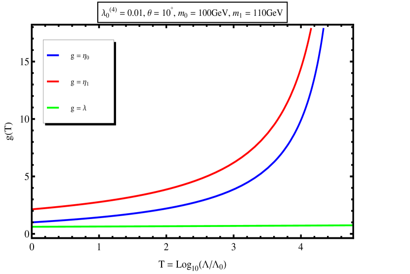
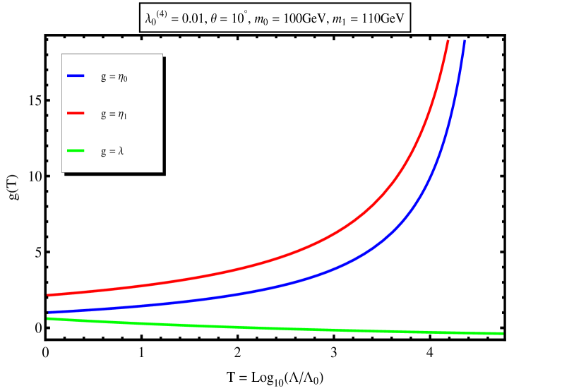
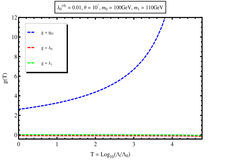
Increasing the dark-matter mass does affect the running of the couplings. Figs. 3 (self-couplings) and 4 (mutual couplings) display such effects for $m_{0}=100\mathrm{GeV}$. Among the self-couplings, $\eta_{1}$ is still dominant, but tailed more closely by $\eta_{0}$ this time. For both, the positive acceleration is accentuated, something that makes $\eta_{1}$ leave the perturbativity region much earlier, at about $6.3\mathrm{TeV}$. By contrast, the running of the Higgs self-coupling $\lambda$ stays flat.

Figure 4: Running of the mutual couplings (scalars only) for a larger DM mass. $\eta_{01}$ starts above 1, much higher than the two others, even higher than the self-coupling $\eta_{1}$.

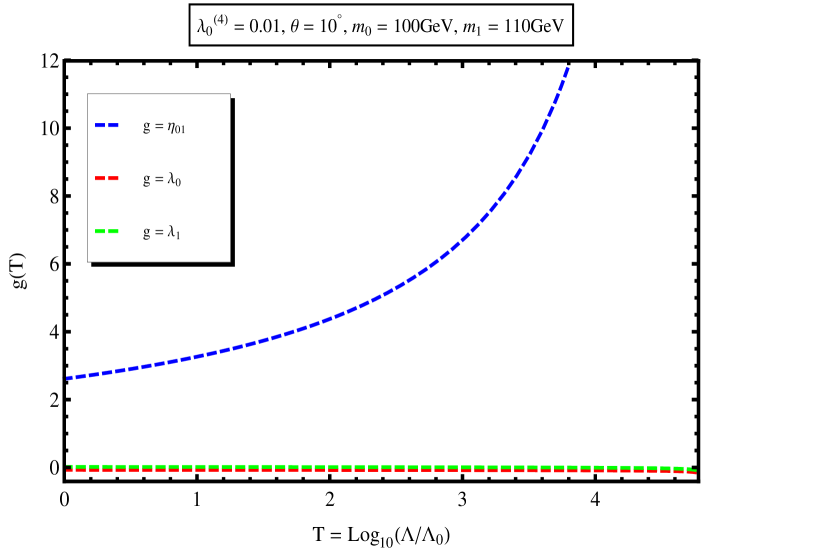
The major effect of increasing $m_{0}$ is on the mutual coupling $\eta_{01}$, between the DM field $S_{0}$ and the auxiliary field $\chi_{1}$. Indeed, in Fig. 2 where $m_{0}=55\mathrm{GeV}$, $\eta_{01}$ started and ran small like the other two mutual couplings. Here, whereas $\lambda_{0}$ and $\lambda_{1}$ (both Higgs related) stay close to zero, $\eta_{01}$ starts above 2.5 and runs up fast. In fact, for these values of the parameters, it leaves the perturbativity region earlier than $\eta_{1}$, at about $2.5\mathrm{TeV}$.

Figure 5: Running of the self-couplings (scalars only) with a larger physical Higgs self-coupling $\lambda_{0}^{(4)}$. The self-coupling $\eta_{1}$ is still dominant.

Increasing the auxiliary-field mass $m_{1}$ has a similar effect: it enhances the positive acceleration of the self-couplings $\eta_{1}$ and $\eta_{0}$ while leaving $\lambda$ flat, and boosts up the mutual coupling $\eta_{01}$ away from $\lambda_{0}$ and $\lambda_{1}$, which both remain not far from zero. It also makes $\eta_{1}$ and $\eta_{01}$ leave the perturbativity region earlier, without $\eta_{01}$ necessarily taking over from $\eta_{1}$.

Increasing $\lambda_{0}^{(4)}$ has also an effect. Figs. 5 (self) and 6 (mutual) show the running for $\lambda_{0}^{(4)}=0.4$. The self-coupling $\eta_{1}$ dominates and leaves the perturbativity region at about $251\mathrm{TeV}$. The mutual coupling $\eta_{01}$ is raised above 1 at $\Lambda_{0}$ and so can run high, while $\lambda_{0}$ and $\lambda_{1}$ stay here too just above zero. It leaves the perturbativity region at about $794\mathrm{GeV}$, well behind $\eta_{1}$. Higher values of $\lambda_{0}^{(4)}$ are more difficult to achieve as the relic-density constraint (5) may not be satisfied abada-ghaffor-nasri .

Figure 6: Running of mutual couplings (scalars only). Larger $\lambda_{0}^{(4)}$ helps $\eta_{01}$ rise well above $\lambda_{0}$ and $\lambda_{1}$, but not enough to win over the self-coupling $\eta_{1}$.

Finally, changing the mixing angle $\theta$ has little effect on the self-coupling constants. It helps the mutual coupling constants $\eta_{01}$ and $\lambda_{1}$ start higher, but not by much: they stay with $\lambda_{0}$ well below one.

IV The full RGE

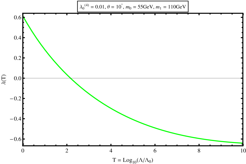
In the previous situation, ‘scalars only’, all running coupling constants were positive, and so there were no issues related to vacuum stability. We now reintroduce the other SM particles and see their effects. Fig. 7 displays the behavior of the self-couplings under the full RGE for the same values of the parameters as in Fig. 1 (scalars only). The dramatic effect is on the Higgs self-coupling constant $\lambda$ which quickly gets into negative territory, at about $15\mathrm{TeV}$, thus rendering the theory unstable beyond this mass scale. This is better displayed in Fig. 8 where the RG behavior of $\lambda$ is shown by itself. Such a negative slope for $\lambda$ is expected, given the negative contributions to $\beta_{\lambda}$ in (2). Here too $\eta_{1}$ is dominant over the other couplings and still controls perturbativity, leaving its region much later, at about $1600~{}\mathrm{TeV}$, farther away from the situation ‘scalars only’. This looks to be a somewhat general trend: the non-Higgs SM particles seem to flatten the runnings of the scalar couplings.

Figure 7: Running of the self-couplings (full RGE). $\eta_{1}$ controls perturbativity and the Higgs coupling $\lambda$ becomes negative quickly.

Figure 8: The running of the Higgs self-coupling $\lambda$ (full RGE). It gets negative at about $15\mathrm{TeV}$ for this set of parameters’ values.

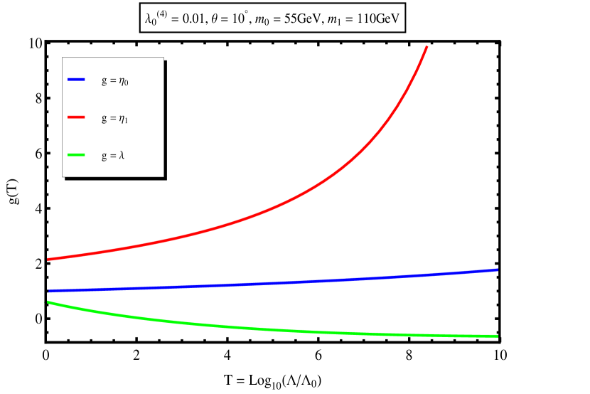
The runnings of the mutual coupling constants for the same set of parameters’ values is displayed in Fig. 9. They also get flattened by the other SM particles, but they stay positive. Here too they dwell well below the self-couplings, as in the ‘scalars only’ case. In fact, many of the effects on the running coupling constants coming from varying the parameters are similar to those of the previous situation since the SM particles do not intervene in the initial values of the couplings (self and mutual) at $\Lambda_{0}$. This means that increasing $m_{0}$ and $m_{1}$ will raise the mutual coupling $\eta_{01}$ and not the two others, higher than $\eta_{1}$ in some regions. For example, Fig. 10 shows the running of the self-couplings when $m_{0}=100\mathrm{GeV}$. Both $\eta_{1}$ and $\eta_{0}$ run faster but $\lambda$ is little affected. Fig. 11 shows the running of the mutual couplings from the full RGE also at $m_{0}=100\mathrm{GeV}$. As in the case ‘scalars only’, larger $m_{0}$ boosts up $\eta_{01}\left(\Lambda_{0}\right)$, much higher than $\lambda_{0}$ and $\lambda_{1}$, at about 2.2 here, which makes it run quickly high, leaving the perturbativity region before $\eta_{1}$, as in the case ‘scalars only’.

Figure 9: Running of the mutual couplings (full RGE). The inclusion of the other SM particles flattens the runnings.

Figure 10: Running of the self-couplings (full RGE) with $m_{0}$ larger. $\eta_{1}$ is more closely tailed by $\eta_{0}$ and $\lambda$ decreases and turns negative at about 10TeV.

Figure 11: Running of the mutual couplings (full RGE) with $m_{0}$ larger. $\eta_{01}$ starts well above $\lambda_{0}$ and $\lambda_{1}$ and leaves the perturbativity region before the self-coupling $\eta_{1}$.

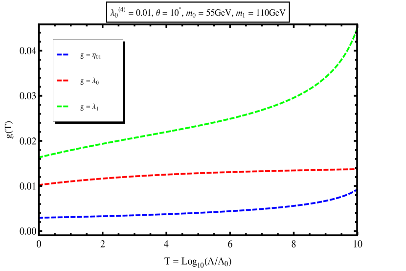
Raising $\lambda_{0}^{(4)}$ will also make the self-couplings $\eta_{1}$ and $\eta_{0}$ run faster while affecting very little $\lambda$. It will also make the mutual coupling $\eta_{01}$ starts higher, and so demarked from $\lambda_{0}$ and $\lambda_{1}$. By contrast, the effect of $\theta$ is not very dramatic: the self-couplings are not much affected and the mutuals only evolve differently, without any particular boosting of $\eta_{01}$.

V Regions of Viability

The foregoing discussion showed us how the scalar parameters of the two-singlet model behave as a function of the mass scale $\Lambda$. From the situation ‘scalars only’ we understood that the two couplings that control perturbativity are $\eta_{1}$ and $\eta_{01}$. The full RGE brought in stability: the change of sign of $\lambda$ is the vacuum stability criterion to use. Equipped with these indicators, we can try to investigate in a more systematic way the viability regions of the model, regions in the space of parameters in which the model is predictive. Remember that this model has four parameters: the dark-matter mass $m_{0}$, the physical auxiliary field mass $m_{1}$, the physical Higgs self-coupling $\lambda_{0}^{(4)}$, and the mixing angle $\theta$ between the physical Higgs and the auxiliary field. The way we proceed is to vary $\lambda_{0}^{(4)}$ and $\theta$ and try to find the regions of viability of the model in the $\left(m_{0},m_{1}\right)$-plane.

We have by now a number of tools at our disposal. First the DM relic-density constraint (5), which has been applied throughout and will continue so. We have the RGE analysis of this work. We will require both $\eta_{1}\left(\Lambda\right)$ and $\eta_{01}\left(\Lambda\right)$ to be smaller than $\sqrt{4\pi}$, and $\lambda\left(\Lambda\right)$ to be positive.

Figure 12: Regions of viability of the two-singlet model (in blue). Physical Higgs self-coupling $\lambda_{0}^{(4)}$ and mixing angle $\theta$ very small.

There is one important issue to address though before we proceed, and that is how far we want the model to be perturbatively predictive and stable. The maximum value $\Lambda_{m}$ for the mass scale $\Lambda$ should not be very high for two reasons. One, more conceptual, is that we want to recognize and allow the model to be intermediary between the Standard Model and some possible higher structure. The second reason, more practical, is that a too-high $\Lambda_{m}$ is too restrictive for the parameters themselves. For example, for the parameters we used in the previous sections, in particular $m_{0}=55\mathrm{GeV}$ and $m_{1}=110~{}\mathrm{GeV}$, we have seen that $\lambda$ gets negative already for $\Lambda\simeq 15\mathrm{TeV}$ whereas $\eta_{1}$ leaves the perturbativity region much later, for $\Lambda\simeq 1600\mathrm{TeV}$. The situation can be reversed. For example, for $m_{0}=67\mathrm{GeV}$, $m_{1}=135\mathrm{GeV}$, and $\theta=15^{\mathrm{o}}$, $\lambda$ can live positive until about $400\mathrm{TeV}$ whereas $\eta_{1}$ leaves perturbativity at about $50\mathrm{TeV}$. In this section, we set $\Lambda_{m}\simeq 40\mathrm{TeV}$.

Figure 13: Regions of viability (blue) of the model. $\lambda_{0}^{(4)}$ still very small, but $\theta$ larger. The region is richer, but not relocated.

As a third viability tool, we want the model to comply with the measured direct-detection upper bounds. In our model, the total cross section for non-relativistic elastic scattering of a dark matter WIMP off a nucleon target is given by the relation abada-ghaffor-nasri :

$$\sigma_{\det}=\frac{m_{N}^{2}\left(m_{N}-\frac{7}{9}m_{B}\right)^{2}}{4\pi\left(m_{N}+m_{0}\right)^{2}v^{2}}\left[\frac{\lambda_{0}^{\left(3\right)}\cos{\theta}}{m_{h}^{2}}-\frac{\eta_{01}^{\left(3\right)}\sin{\theta}}{m_{1}^{2}}\right]^{2}.$$ (8)

In this relation, $m_{N}$ is the nucleon mass and $m_{B}$ the baryon mass in the chiral limit. The quantities $\lambda_{0}^{\left(3\right)}$ and $\eta_{01}^{\left(3\right)}$ are coupling constants of cubic terms in the theory after spontaneous breaking of the two symmetries abada-ghaffor-nasri :

$$\lambda_{0}^{\left(3\right)}=\lambda_{0}\cos\theta+\eta_{01}v_{1}\sin\theta;\quad\eta_{01}^{\left(3\right)}=\eta_{01}v_{1}\cos\theta-\lambda_{0}v\sin\theta.$$ (9)

The condition we impose is that $\sigma_{\det}$ be within the XENON 100 upper-bounds XENON100 .

In work abada-nasri-1 , we studied phenomenological implications of the model and constraints on it, using rare meson decays and Higgs production. A number of inferences were deduced, but we will prefer to retain only two. One is that the mixing angle $\theta$ is to be chosen small. This is emphasized in view of the mounting evidence of a SM Higgs particle found by ATLAS and CMS at the LHC ATLAS ; CMS . The other is that the physical self-coupling $\lambda_{0}^{(4)}$ is to be small too. This was already observed in abada-ghaffor-nasri , where the relic-density constraint has the tendency of ‘shutting down’ high values of $\lambda_{0}^{(4)}$. At the end of the next section, we will comment on possible larger values for $\lambda_{0}^{(4)}$.

Figure 14: The region of viability (blue) is even richer for larger mixing angle $\theta$.

In this section, the display range of $m_{0}$ and $m_{1}$ is from $1\mathrm{GeV}$ to $160\mathrm{GeV}$. Indeed, there is no reliable data to discuss regarding a dark-matter mass below the GeV, and in view of the behavior of $\eta_{1}$ at $\Lambda_{0}$ as a function of $m_{1}$, taking this latter beyond $160\mathrm{GeV}$ is outside the perturbativity region. In practice, $m_{0}$ was taken up to $200\mathrm{GeV}$, with no additional features to report.

Let us start with $\lambda_{0}^{(4)}$ and $\theta$ both very small. Fig. 12 displays the regions (blue) for which the model is viable up to $\Lambda_{m}\simeq 40\mathrm{TeV}$. Here $\lambda_{0}^{(4)}=0.01$ and $\theta=1^{\mathrm{o}}$. We see that the mass $m_{1}$ is confined to the interval $116\mathrm{GeV}-138\mathrm{GeV}$. The dark-matter mass is confined mainly to the region above $118\mathrm{GeV}$, the left boundary of which having a positive slope as $m_{1}$ increases. The DM mass $m_{0}$ has also a small showing in the narrow interval $57\mathrm{GeV}-68\mathrm{GeV}$.

The effect of increasing the mixing angle $\theta$ is to enrich the existing regions without relocating them. This is displayed in Figs. 13 and 14 for which $\theta$ is increased to $5^{\mathrm{o}}$ and $15^{\mathrm{o}}$ respectively. We see that, as $\theta$ increases, the region between the narrow band and the larger one to the right gets populated. This means more dark-matter masses above $60\mathrm{GeV}$ are allowed, but $m_{1}$ stays in the same interval, roughly $116\mathrm{GeV}-138\mathrm{GeV}$.

Figure 15: The physical Higgs self-coupling $\lambda_{0}^{(4)}$ shrinks the viability region (blue) as it increases.

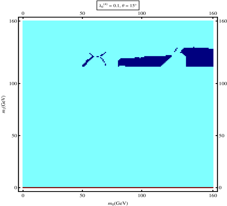
Increasing the Higgs-DM mutual coupling $\lambda_{0}^{\left(4\right)}$ has the opposite effect, that of shrinking existing viability regions. Indeed, compare Fig. 15 for which $\lambda_{0}^{\left(4\right)}=0.1$ and $\theta=15^{\mathrm{o}}$ $\left(\Lambda_{m}\simeq 40\mathrm{TeV}\right)$ with Fig. 14. We see shrunk regions, pushed downward by a few GeVs, which is not a substantial relocation. Remember that increasing $\lambda_{0}^{\left(4\right)}$ raises $\eta_{01}\left(\Lambda_{0}\right)$ well enough above 1 so that this latter will leave the perturbativity region sooner. Increasing it is also caught up by the relic-density constraint, which tends to shut down such larger values of $\lambda_{0}^{\left(4\right)}$ when the dark-matter mass $m_{0}$ is large. The direct-detection constraint has also a similar effect.

VI Concluding remarks

In this work, we have studied the effects and consequences of the renormalization group equations at one-loop order on a two-singlet model of cold dark matter that consists in extending the Standard Model with two real gauge-singlet scalar fields. The two issues we monitored are perturbativity and vacuum stability. The former is controlled by the auxiliary-field self-coupling $\eta_{1}$ and the mutual coupling $\eta_{01}$ between the dark matter and the auxiliary fields. The latter is controlled by the Higgs self-coupling $\lambda$. When the non-Higgs SM coupling constants are switched off, all scalar couplings are positive increasing functions of the scale $\Lambda$. Reintroducing them flattens the rates for all the scalar couplings and makes the Higgs coupling $\lambda$ turn negative at some scale. The mutual couplings $\lambda_{0}$ (DM-Higgs) and $\lambda_{1}$ (Higgs-auxiliary) stay always well below one, whereas $\eta_{01}$ boosts up for larger $m_{0}$ (DM mass) and/or $m_{1}$ (auxiliary-field mass), dominating over $\eta_{1}$ in some regions.

We then have investigated the regions in the space of parameters in which the model is viable. We have plotted these regions in the ($m_{0},m_{1}$)-plane while varying the physical mutual coupling $\lambda_{0}^{(4)}$ between the dark matter $S_{0}$ and the physical Higgs $h$, and the mixing angle $\theta$ between $h$ and the physical auxiliary field. We have required that the model reproduces the DM relic density abundance, and that it complies with the measured direct-detection upper bounds – those of the XENON 100 experiment. We have also imposed the RGE perturbativity and vacuum-stability criteria that we deduced from this work together with a maximum cutoff $\Lambda_{m}\simeq 40\mathrm{TeV}$, a scale at which heavy degrees of freedom may start to be relevant, something that could be probed by future colliders. This analysis has shown that for small $\lambda_{0}^{(4)}$ and $\theta$, the auxiliary-field mass $m_{1}$ is confined to the interval $116\mathrm{GeV}-138\mathrm{GeV}$, while the DM mass $m_{0}$ is confined mainly to the region above $118\mathrm{GeV}$, with a small showing in the narrow interval $57\mathrm{GeV}-68\mathrm{GeV}$. Increasing $\theta$ enriches the existing viability regions without relocating them, while increasing$\ \lambda_{0}^{\left(4\right)}$ has the opposite effect, that of shrinking them without substantial relocation.

It is pertinent at this stage to comment on the implications of the Higgs discovery at the LHC on the possibility of having a light dark matter WIMP $S_{0}$ with a mass $m_{0}\lesssim 62\mathrm{GeV}$, a situation allowed in this two-singlet model. Indeed, on the one hand, for such a light dark matter, the decay channel $h\rightarrow S_{0}S_{0}$ becomes open, and therefore will lower the number of Higgs decays into SM particles. On the other hand, The ATLAS and CMS published data on Higgs boson searches seem to indicate that the observed boson is SM-like, and so, one expects to have stringent constraints on the parameter space when it comes to light dark-matter masses. In GKMRS , a global fit to the Higgs boson data that includes those presented at the Moriond 2013 conference by the ATLAS and CMS collaborations ATLAS2013 ; CMS2013 has been performed; see GFIT for earlier fits. It has been found that any extra invisible Higgs boson decay must be bounded by the following condition on the corresponding branching ratio:

$$\mathrm{Br}(h\rightarrow\mathrm{invisible})<19\%.$$ (10)

It turns out that in our two-singlet model, the branching fraction of the invisible width of the Higgs boson is smaller than the bound above for $m_{0}\lesssim 62\mathrm{GeV}$. Indeed, if we take for example $m_{0}=55\mathrm{GeV}$ used frequently in this work, the ratio $\Gamma(h\rightarrow S_{0}S_{0})/{\Gamma(h\rightarrow b{\bar{b}})}$ is less than $17\%$, quite consistent with the above current bound. Therefore, we conclude that the two-singlet model is consistent with the current available data regarding the Higgs boson searches.

Finally, we ask whether the model allows for very light cold dark matter. Below $5\mathrm{GeV}$, direct detection puts no experimental bound on the total cross section $\sigma_{\det}$ for non-relativistic elastic scattering of a dark matter WIMP off a nucleon target. Such a situation allows for very small $m_{0}$ regions of viability, but only when $\lambda_{0}^{\left(4\right)}$ is quite large ($\sim 2$ and above) and $\theta$ not too small ( $\sim 15^{\mathrm{o}}$ and above). However, for such values of the parameters, the branching fraction of the invisible Higgs decay is larger than $25\%$, which is excluded by the current LHC available data.

References

- (1) G. Aad et al. [ATLAS Collaboration], Phys. Lett. B 716, 1 (2012).
- (2) S. Chatrchyan et al. [CMS Collaboration], Phys. Lett. B 716, 30 (2012).
- (3) P.A.R. Ade et al. [Planck Collaboration], arXiv:1303.5062 [astro-ph.CO].
- (4) V. Silveira and A. Zee, Phys. Lett. B 161, 136 (1985).
- (5) J. McDonald, Phys. Rev. D 50, 3637 (1994).
- (6) C. P. Burgess, M. Pospelov, and T. ter Veldhuis, Nucl. Phys. B 619, 709 (2001).
- (7) C. Bird, P. Jackson, R. V. Kowalewski, and M. Pospelov, Phys. Rev. Lett. 93, 201803 (2004); D. O’Connell, M.J. Ramsey-Musolf, and M.B. Wise, Phys. Rev. D 75, 037701 (2007); V. Barger, P. Langacker, M. McCaskey, M. J. Ramsey-Musolf, and G. Shaughnessy, Phys. Rev. D 77, 035005 (2008); X.G. He, T. Li, X.Q. Li, J. Tandean, and H.C. Tsai, Phys. Rev. D 79, 023521 (2009); M. Gonderinger, Y. Li, H. Patel, and M.J. Ramsey-Musolf, JHEP 01 (2010) 053; S. Andreas, C. Arina, T. Hambye, F-S. Ling, and M.H.G. Tytgat, Phys. Rev. D 82, 043522 (2010); Y. Cai, X. G. He, and B. Ren, Phys. Rev. D 83, 083524 (2011); J.M. Cline, K. Kainulainen, JCAP 1301, 012 (2013).
- (8) A. Djouadi, O. Lebedev, Y. Mambrini, and J. Quevillon, Phys. Lett. B 709, 65 (2012).
- (9) J. Angle et al. [XENON Collaboration], Phys. Rev. Lett. 100, 021303 (2008).
- (10) Z. Ahmed et al. [CDMS Collaboration], Phys. Rev. Lett. 102, 011301 (2009); Science 327, 1619 (2010).
- (11) E. Aprile et al. [XENON100 Collaboration], Phys. Rev. Lett. 109, 181301 (2012).
- (12) G. Belanger, B. Dumont, U. Ellwanger, J. F. Gunion, and S. Kraml, arXiv:1302.5694 [hep-ph].
- (13) See also M. Asano and R. Kitano, Phys. Rev. D 81, 054506 (2010); Y. Mambrini, Phys. Rev. D 84, 115017 (2011); M. Farina, M. Kadastik, D. Pappadopulo, J. Pata, M. Raidal, and A. Strumia, Nucl. Phys. B 853, 607 (2011); I. Low, P. Schwaller, G. Shaughnessy, and C.E.M. Wagner, Phys. Rev. D 85, 015009 (2012); Y. Mambrini, J. Phys. Conf. Ser. 375, 012045 (2012).
- (14) A. Abada, D. Ghaffor, and S. Nasri, Phys. Rev. D 83, 095021 (2011).
- (15) A. Abada and S. Nasri, Phys. Rev. D 85, 075009 (2012).
- (16) M. Gonderinger, H. Lim, and M.J. Ramsey-Musolf, Phys. Rev. D 86, 043511 (2012).
- (17) C. Ford, D.R.T. Jones, P.W. Stephenson, and M.B. Einhorn, Nucl. Phys. B 395, 17 (1993); M. Sher, Phys. Rept. 179, 273 (1989); A. Djouadi, Phys. Rept. 457, 1 (2008).
- (18) P.A.R. Ade et al. [Planck Collaboration], arXiv:1303.5076 [astro-ph.CO].
- (19) P.P. Giardino, K. Kannike, I. Masina, M. Raidal, and A. Strumia, arXiv:1303.3570 [hep-ph].
- (20) V. Martin, Talk presented at Rencontres de Moriond - 2-16 March 2013, La Thuile.
- (21) C. Ochando, Talk presented at Rencontres de Moriond - 2-16 March 2013, La Thuile.
- (22) G. Belanger, B. Dumont, U. Ellwanger, J. F. Gunion, and S. Kraml, arXiv:1302.5694 [hep-ph]; P.P. Giardino, K. Kannike, M. Raidal, and A. Strumia, JHEP 1206, 117 (2012); J.R. Espinosa, M. Muhlleitner, C. Grojean, and M. Trott, JHEP 1209, 126 (2012).