Determining White Noise Forcing From Eulerian Observations in the Navier-Stokes Equation

Abstract

The Bayesian approach to inverse problems is of paramount importance in quantifying uncertainty about the input to, and the state of, a system of interest given noisy observations. Herein we consider the forward problem of the forced 2D Navier-Stokes equation. The inverse problem is to make inference concerning the forcing, and possibly the initial condition, given noisy observations of the velocity field. We place a prior on the forcing which is in the form of a spatially-correlated and temporally-white Gaussian process, and formulate the inverse problem for the posterior distribution. Given appropriate spatial regularity conditions, we show that the solution is a continuous function of the forcing. Hence, for appropriately chosen spatial regularity in the prior, the posterior distribution on the forcing is absolutely continuous with respect to the prior and is hence well-defined. Furthermore, it may then be shown that the posterior distribution is a continuous function of the data. We complement these theoretical results with numerical simulations showing the feasibility of computing the posterior distribution, and illustrating its properties.

1 Introduction

The Bayesian approach to inverse problems has grown in popularity significantly over the last decade, driven by algorithmic innovation and steadily increasing computer power kaipio2004statistical . Recently there have been systematic developments of the theory of Bayesian inversion on function space La02 ; La07 ; CDRS ; stuart2010inverse ; lasanen2012non ; lasanen2012nonb and this has led to new sampling algorithms which perform well under mesh-refinement CRSW12 ; vollmer2013 ; law2012proposals . In this paper we add to this growing interest in the Bayesian formulation of inversion, in the context of a specific PDE inverse problem, motivated by geophysical applications such as data assimilation in the atmosphere and ocean sciences, and demonstrate that fully Bayesian probing of the posterior distribution is feasible.

The primary goal of this paper is to demonstrate that the Bayesian formulation of inversion for the forced Navier-Stokes equation, introduced in CDRS , can be extended to the case of white noise forcing. The paper CDRS assumed an Ornstein-Uhlenbeck structure in time for the forcing, and hence did not include the white noise case. It is technically demanding to extend to the case of white noise forcing, but it is also of practical interest. This practical importance stems from the fact that the Bayesian formulation of problems with white noise forcing corresponds to a statistical version of the continuous time weak constraint 4DVAR methodology zupanski1997general . The 4DVAR approach to data assimilation currently gives the most accurate global short term weather forecasts available lorenc2003potential and this is arguably the case because, unlike ensemble filters which form the major competitor, 4DVAR has a rigorous statistical interpretation as a maximum a posteriori (or MAP) estimator – the point which maximizes the posterior probability. It is therefore of interest to seek to embed our understanding of such methods in a broader Bayesian context.

To explain the connection between our work and the 4DVAR methodology and, in particular, to explain the terminology used in the data assimilation community, it is instructive to consider the finite dimensional differential equation

$$\frac{du}{dt}=f(u)+\xi,\quad u(0)=u_{0}$$

on $\mathbb{R}^{n}$. Assume that we are given noisy observations $\{y_{j}\}$ of the solution $u_{j}=u(t_{j})$ at times $t_{j}=jh$ so that

$$y_{j}=u_{j}+\eta_{j},\quad j=1,\cdots,J,$$

for some noises $\eta_{j}.$ An important inverse problem is to determine the initial condition $u_{0}$ and forcing $\xi$ which best fits the data. If we view the solution $u_{j}$ as a function of the initial condition and forcing, then a natural regularized least squares problem is to determine $u_{0}$ and $\xi$ to minimize

$$I(u_{0},\xi)=\sum_{j=1}^{J}\Bigl{|}\Gamma^{-\frac{1}{2}}\bigl{(}y_{j}-u_{j}(u_{0},\xi)\bigr{)}\Bigr{|}^{2}+|\Sigma^{-\frac{1}{2}}u_{0}|^{2}+\|\mathsf{Q}^{-\frac{1}{2}}\xi\|^{2}$$

where $|\cdot|,\|\cdot\|$ denote the $\mathbb{R}^{n}-$Euclidean and $L^{2}\bigl{(}[0,T];\mathbb{R}^{n}\bigr{)}$ norms respectively, $\Gamma,\Sigma$ denote covariance matrices and $\mathsf{Q}$ a covariance operator. This is a continuous time analogue of the 4DVAR or variational methodology, as described in the book of Bennett bennett2002inverse . In numerical weather prediction the method is known as weak constraint 4DVAR, and as 4DVAR if $\xi$ is set to zero (so that the ODE

$$\frac{du}{dt}=f(u),\quad u(0)=u_{0}$$

is satisfied as a hard constraint), the term $\|\mathsf{Q}^{-\frac{1}{2}}\xi\|^{2}$ dropped, and the minimization is over $u_{0}$ only. As explained in kaipio2004statistical , these minimization problems can be viewed as probability maximizers for the posterior distribution of a Bayesian formulation of the inverse problem – the so-called MAP estimators. In this interpretation the prior measures on $u_{0}$ and $\xi$ are centred Gaussians with covariances $\Sigma$ and $\mathsf{Q}$ respectively. Making this connection opens up the possibility of performing rigorous statistical inversion, and thereby estimating uncertainty in predictions made.

The ODEs arising in atmosphere and ocean science applications are of very high dimension, arising from discretizations of PDEs. It is therefore conceptually important to carry through the program in the previous paragraph, and in particular Bayesian formulation of the inversion, for PDEs; the paper dashti2013map explains how to define MAP estimators for measures on Hilbert spaces and the connection to variational problems. The Navier-Stokes equation in 2D provides a useful canonical example of a PDE of direct relevance to the atmosphere and ocean sciences. When the prior covariance operator $\mathsf{Q}$ is chosen to be that associated to an Ornstein-Uhleneck operator in time, the Bayesian formulation for the 2D Navier-Stokes equation has been carried out in CDRS . Our goal in this paper is to extend to the more technically demanding case where $\mathsf{Q}$ is the covariance operator associated with a white noise in time, with spatial correlations $Q$. We will thus use the prior model $\xi dt={dW}$ where $W$ is a $Q-$Wiener process in an appropriate Hilbert space, and consider inference with respect to $W$ and $u_{0}.$ In the finite dimensional setting the differences between the case of coloured and white noise forcing, with respect to the inverse problem, are much less substantial and the interested reader may consult HSV11 for details.

The key tools required in applying the function space Bayesian approach in stuart2010inverse are the proof of continuity of the forward map from the function space of the unknowns to the data space, together with estimates of the dependence of the forward map upon its point of application, sufficient to show certain integrability properties with respect to the prior. This program is carried out for the 2D Navier-Stokes equation with Ornstein-Uhlenbeck priors on the forcing in the paper CDRS . However to use priors which are white in time adds further complications since it is necessary to study the stochastically forced 2D Navier-Stokes equation and to establish continuity of the solution with respect to small changes in the Brownian motion $W$ which defines the stochastic forcing. We do this by employing the solution concept introduced by Flandoli in Flandoli94 , and using probabilistic estimates on the solution derived by Mattingly in Mattingly99 . In section 2 we describe the relevant theory of the forward problem, employing the setting of Flandoli. In section 3 we build on this theory, using the estimates of Mattingly to verify the conditions in stuart2010inverse , resulting in a well-posed Bayesian inverse problem for which the posterior is Lipschitz in the data with respect to Hellinger metric. Section 4 extends this to include making inference about the initial condition as well as the forcing. Finally, in section 5, we present numerical results which demonstrate feasibility of sampling from the posterior on white noise forces, and demonstrate the properties of the posterior distribution.

2 Forward Problem

In this section we study the forward problem of the Navier-Stokes equation driven by white noise. Subsection 2.1 describes the forward problem, the Navier-Stokes equation, and rewrites it as an ordinary differential equation in a Hilbert space. In subsection 2.2 we define the functional setting used throughout the paper. Subsection 2.3 highlights the solution concept that we use, leading in subsection 2.4 to proof of the key fact that the solution of the Navier-Stokes equation is continuous as a function of the rough driving of interest and the initial condition. All our theoretical results in this paper are derived in the case of Dirichlet (no flow) boundary conditions. They may be extended to the problem on the periodic torus $\mathbb{T}^{d}$, but we present the more complex Dirichlet case only for brevity.

2.1 Overview

Let $D\in\mathbb{R}^{2}$ be a bounded domain with smooth boundary. We consider in $D$ the Navier-Stokes equation

$$\partial_{t}u-\nu\Delta u+u\cdot\nabla u = f-\nabla p,\quad(x,t)\in D\times(0,\infty)$$ (1)

$$\nabla\cdot u = 0,\quad(x,t)\in D\times(0,\infty)$$

$$u = 0,\quad(x,t)\in\partial D\times(0,\infty),$$

$$u = u_{0},\quad(x,t)\in D\times\{0\}.$$

We assume that the initial condition $u_{0}$ and the forcing $f(\cdot,t)$ are divergence-free. We will in particular work with equation $(\ref{eq:u})$ below, obtained by projecting $(\ref{eq:NSE})$ into the space of divergence free functions – the Leray projector temam1984navier . We denote by $\mathsf{V}$ the space of all divergence-free smooth functions from $D$ to $\mathbb{R}^{2}$ with compact support, by $\mathbb{H}$ the closure of $\mathsf{V}$ in $(L^{2}(D))^{2}$, and by $\mathbb{H}^{1}$ the closure of $\mathsf{V}$ in $(H^{1}(D))^{2}$. Let $\mathbb{H}^{2}=(H^{2}(D))^{2}\bigcap\mathbb{H}^{1}$. The initial condition $u_{0}$ is assumed to be in $\mathbb{H}$. We define the linear Stokes’ operator $A:\mathbb{H}^{2}\to\mathbb{H}$ by $Au=-\Delta u$ noting that the assumption of compact support means that Dirichlet boundary condition are imposed on the Stokes’ operator $A$. Since $A$ is selfadjoint, $A$ possesses eigenvalues $0<\lambda_{1}\leq\lambda_{2}\leq\ldots$ with the corresponding eigenvectors $e_{1},e_{2},\ldots\in\mathbb{H}^{2}$.

We denote by $\langle\cdot,\cdot\rangle$ the inner product in $\mathbb{H}$, extended to the dual pairing on $\mathbb{H}^{-1}\times\mathbb{H}^{1}$. We then define the bilinear form $B:\mathbb{H}^{1}\times\mathbb{H}^{1}\to\mathbb{H}^{-1}$

$$\langle B(u,v),z\rangle=\int_{D}z(x)\cdot(u(x)\cdot\nabla)v(x)dx$$

which must hold for all $z\in\mathbb{H}^{1}.$ From the incompressibility condition we have, for all $z\in\mathbb{H}^{1}$,

$$\langle B(u,v),z\rangle=-\langle B(u,z),v\rangle.$$ (2)

By projecting problem $(\ref{eq:NSE})$ into $\mathbb{H}$ we may write it as an ordinary differential equation in the form

$$du(t)=-\nu Audt-B(u,u)dt+dW(t),\ \ u(0)=u_{0}\in\mathbb{H},$$ (3)

where $dW(t)$ is the projection of the forcing $f(x,t)dt$ into $\mathbb{H}$. We will define the solution of this equation pathwise, for suitable $W$, not necessarily differentiable in time.

2.2 Function Spaces

For any $s\geq 0$ we define $\mathbb{H}^{s}\subset\mathbb{H}$ to be the Hilbert space of functions $u=\sum_{k=1}^{\infty}u_{k}e_{k}\in\mathbb{H}$ such that

$$\sum_{k=1}^{\infty}\lambda_{k}^{s}u_{k}^{2}<\infty;$$

we note that the $\mathbb{H}^{j}$ for $j\in\{0,1,2\}$ coincide with the preceding definitions of these spaces. The space $\mathbb{H}^{s}$ is endowed with the inner product

$$\langle u,v\rangle_{\mathbb{H}^{s}}=\sum_{k=1}^{\infty}\lambda_{k}^{s}u_{k}v_{k},$$

for $u=\sum_{k=1}^{\infty}u_{k}e_{k}$, $v=\sum_{k=1}^{\infty}v_{k}e_{k}$ in $\mathbb{H}$. We denote by $\mathbb{V}$ the particular choice $s=\frac{1}{2}+\epsilon$, namely $\mathbb{H}^{\frac{1}{2}+\epsilon}$, for given $\epsilon>0$. In what follows we will be particularly interested in continuity of the mapping from the forcing $W$ into linear functionals of the solution of $(\ref{eq:u})$. To this end it is helpful to define the Banach space ${\mathbb{X}}:=C([0,T];\mathbb{V})$ with the norm

$$\|W\|_{{\mathbb{X}}}=\sup_{t\in(0,T)}\|W(t)\|_{\mathbb{V}}.$$

2.3 Solution Concept

In what follows we define a solution concept for equation $(\ref{eq:u})$ for each forcing function $W$ which is continuous, but not necessarily differentiable, in time. We always assume that $W(0)=0.$ Following Flandoli Flandoli94 , for each $W\in{\mathbb{X}}$ we define the weak solution $u(\cdot;W)\in C([0,T];\mathbb{H})\bigcap L^{2}([0,T];\mathbb{H}^{1/2})$ of $(\ref{eq:u})$ as a function that satisfies

$$\langle u(t),\phi\rangle+{\nu}\int_{0}^{t}\langle u(s),A\phi\rangle ds-\int_{0}^{t}\langle{B\bigl{(}u(s),\phi\bigr{)},u(s)}\rangle dx=\langle u_{0},\phi\rangle+\langle W(t),\phi\rangle,$$ (4)

for all $\phi\in\mathbb{H}^{2}$ and all $t\in(0,T)$; note the integration by parts on the Stokes’ operator and the use of $(\ref{eq:Buvz})$ to derive this identity from $(\ref{eq:u})$. Note further that if $u$ and $W$ are sufficiently smooth, $(\ref{eq:weaksln})$ is equivalent to $(\ref{eq:u})$.

To employ this solution concept we first introduce the concept of a solution of the linear equation

$$dz(t)=-\nu Azdt+dW(t),\ \ z(0)=0\in\mathbb{H}$$ (5)

where $W$ is a deterministic continuous function obtaining values in $\mathbb{X}$ but not necessarily differentiable. We define a weak solution of this equation as a function $z\in C([0,T];\mathbb{H})$ such that

$$\langle z(t),\phi\rangle+{\nu}\int_{0}^{t}\langle z(s),A\phi\rangle ds=\langle W(t),\phi\rangle$$ (6)

for all $\phi\in\mathbb{H}^{2}$.

Then for this function $z(t)$ we consider the solution $v$ of the equation

$$dv(t)=-\nu Avdt-B(z+v,z+v)dt,\ \ v(0)=u_{0}\in\mathbb{H}.$$ (7)

As we will show below, $z(t)$ possesses sufficiently regularity so $(\ref{eq:v})$ possesses a weak solution $v$. We then deduce that $u=z+v$ is a weak solution of $(\ref{eq:u})$ in the sense of $(\ref{eq:weaksln})$. When we wish to emphasize the dependence of $u$ on $W$ (and similarly for $z$ and $v$) we write $u(t;W).$

We will now show that the function $z$ defined by

$$z(t) = \int_{0}^{t}e^{-\nu A(t-s)}dW(s)$$ (8)

$$= W(t)-\int_{0}^{t}\nu Ae^{-\nu A(t-s)}W(s)ds.$$

satisfies the weak formula $(\ref{eq:weakz})$. Let $w_{k}=\langle W,e_{k}\rangle$, that is

$$W(t):=\sum_{k=1}^{\infty}{w_{k}}(t)e_{k}\in{\mathbb{X}}.$$ (9)

We then deduce from $(\ref{eq:zt})$ that

$$z(t;W)=W(t)-\sum_{k=1}^{\infty}\Bigl{(}\int_{0}^{t}w_{k}(s){\nu}\lambda_{k}e^{(t-s)(-{\nu}\lambda_{k})}ds\Bigr{)}e_{k}.$$ (10)

We have the following regularity property for $z$:

Lemma 1

For each $W\in{\mathbb{X}}$, the function $z=z(\cdot;W)\in C([0,T];\mathbb{H}^{1/2})$.

Proof  We first show that for each $t$, $z(t;W)$ as defined in $(\ref{eq:zz})$ belongs to $\mathbb{H}^{1/2}$. Fixing an integer $M>0$, using inequality $a^{1-\epsilon/2}e^{-a}<c$ for all $a>0$ for an appropriate constant $c$, we have

$$\sum_{k=1}^{M}\lambda_{k}^{1/2}\Bigg{(}\int_{0}^{t}\nu\lambda_{k}e^{(t-s)(-\nu\lambda_{k})}w_{k}(s)ds\Bigg{)}^{2}\leq\sum_{k=1}^{M}\lambda_{k}^{1/2}\Bigg{(}\int_{0}^{t}{c\over(t-s)^{1-\epsilon/2}}\lambda_{k}^{\epsilon/2}|w_{k}(s)|dx\Bigg{)}^{2}.$$

Therefore,

$$\Bigg{\|}\sum_{k=1}^{M}\int_{0}^{t}\nu\lambda_{k}e^{(t-s)(-\nu\lambda_{k})}w_{k}(s)e_{k}ds\Bigg{\|}_{\mathbb{H}^{1/2}} \leq \Bigg{\|}\sum_{k=1}^{M}\int_{0}^{t}{c\over(t-s)^{1-\epsilon/2}}\lambda_{k}^{\epsilon/2}|w_{k}(s)|e_{k}ds\Bigg{\|}_{\mathbb{H}^{1/2}}$$

$$\leq \int_{0}^{t}{c\over(t-s)^{1-\epsilon/2}}\Bigg{\|}\sum_{k=1}^{M}\lambda_{k}^{\epsilon/2}|w_{k}(s)|e_{k}\Bigg{\|}_{\mathbb{H}^{1/2}}ds$$

$$\leq \max_{s\in(0,T)}\|W(s)\|_{\mathbb{H}^{1/2+\epsilon}}\int_{0}^{t}{c\over(t-s)^{1-\epsilon/2}}ds,$$

which is uniformly bounded for all $M$. Therefore,

$$\sum_{k=1}^{\infty}\Bigg{(}\int_{0}^{t}w_{k}(s)\nu\lambda_{k}e^{(t-s)(-\nu\lambda_{k})}ds\Bigg{)}e_{k}\in\mathbb{H}^{1/2},$$

It follows from $(\ref{eq:zz})$ that, since $W\in{\mathbb{X}}$, for each $t$, $z(t;W)\in\mathbb{H}^{1/2}$ as required. Furthermore, for all $t\in(0,T)$

$$\|z(t;W)\|_{\mathbb{H}^{1/2}}\leq c\|W\|_{{\mathbb{X}}}.$$ (11)

Now we turn to the continuity in time. Arguing similarly, we have that

$$\Bigg{\|}\sum_{k=M}^{\infty}\Bigg{(}\int_{0}^{t}w_{k}(s)\nu\lambda_{k}e^{(t-s)(-\nu\lambda_{k})}ds\Bigg{)}e_{k}\Bigg{\|}_{\mathbb{H}^{1/2}}\leq\int_{0}^{t}{c\over(t-s)^{1-\epsilon/2}}\Bigg{\|}\sum_{k=M}^{\infty}w_{k}(s)e_{k}\Bigg{\|}_{\mathbb{H}^{1/2+\epsilon}}ds$$

$$\qquad\qquad\leq\Bigg{(}\int_{0}^{t}{c\over(t-s)^{(1-\epsilon/2)^{p}}}ds\Bigg{)}^{1/p}\Bigg{(}\int_{0}^{t}\Bigg{\|}\sum_{k=M}^{\infty}w_{k}(s)e_{k}\Bigg{\|}^{q}_{\mathbb{H}^{1/2+\epsilon}}ds\Bigg{)}^{1/q},$$

for all $p,q>0$ such that $1/p+1/q=1$. From the Lebesgue dominated convergence theorem,

$$\lim_{M\to\infty}\int_{0}^{t}\Bigg{\|}\sum_{k=M}^{\infty}w_{k}(s)e_{k}\Bigg{\|}^{q}_{\mathbb{H}^{1/2+\epsilon}}ds=0;$$

and when $p$ sufficiently close to 1,

$$\int_{0}^{t}{c\over(t-s)^{(1-\epsilon/2)p}}ds$$

is finite. We then deduce that

$$\lim_{M\to\infty}\Bigg{\|}\sum_{k=M}^{\infty}\Bigg{(}\int_{0}^{t}w_{k}(s)\nu\lambda_{k}e^{(t-s)(-\nu\lambda_{k})}ds\Bigg{)}e_{k}\Bigg{\|}_{\mathbb{H}}^{1/2}=0,$$

uniformly for all $t$.

Fixing $t\in(0,T)$ we show that

$$\lim_{t^{\prime}\to t}\|z(t;W)-z({t^{\prime};W})\|_{\mathbb{H}^{1/2}}=0.$$

We have

$$\|z(t;W)-z(t^{\prime};W)\|_{\mathbb{H}^{1/2}}\leq\|W(t)-W(t^{\prime})\|_{\mathbb{H}^{1/2}}+$$

$$\qquad\qquad\Bigg{\|}\sum_{k=1}^{M-1}\Bigg{(}\int_{0}^{t}w_{k}(s)\nu\lambda_{k}e^{(t-s)(-\nu\lambda_{k})}ds-\int_{0}^{t^{\prime}}w_{k}(s)\nu\lambda_{k}e^{(t^{\prime}-s)(-\nu\lambda_{k})}ds\Bigg{)}e_{k}\Bigg{\|}_{\mathbb{H}^{1/2}}+$$

$$\Bigg{\|}\sum_{k=M}^{\infty}\Bigg{(}\int_{0}^{t}w_{k}(s)\nu\lambda_{k}e^{(t-s)(-\nu\lambda_{k})}ds\Bigg{)}e_{k}\Bigg{\|}_{\mathbb{H}^{1/2}}+\Bigg{\|}\sum_{k=M}^{\infty}\Bigg{(}\int_{0}^{t^{\prime}}w_{k}(s)\nu\lambda_{k}e^{(t^{\prime}-s)(-\nu\lambda_{k})}ds\Bigg{)}e_{k}\Bigg{\|}_{\mathbb{H}^{1/2}}.$$

For $\delta>0$, when $M$ is sufficiently large, the argument above shows that

$$\Bigg{\|}\sum_{k=M}^{\infty}\Bigg{(}\int_{0}^{t}w_{k}(s)\nu\lambda_{k}e^{(t-s)(-\nu\lambda_{k})}ds\Bigg{)}e_{k}\Bigg{\|}_{\mathbb{H}^{1/2}}+\Bigg{\|}\sum_{k=M}^{\infty}\Bigg{(}\int_{0}^{t^{\prime}}w_{k}(s)\nu\lambda_{k}e^{(t^{\prime}-s)(-\nu\lambda_{k})}ds\Bigg{)}e_{k}\Bigg{\|}_{\mathbb{H}^{1/2}}<\delta/3.$$

Furthermore, when $|t^{\prime}-t|$ is sufficiently small,

$$\Bigg{\|}\sum_{k=1}^{M-1}\Bigg{(}\int_{0}^{t}w_{k}(s)\nu\lambda_{k}e^{(t-s)(-\nu\lambda_{k})}ds-\int_{0}^{t^{\prime}}w_{k}(s)\nu\lambda_{k}e^{(t^{\prime}-s)(-\nu\lambda_{k})}ds\Bigg{)}e_{k}\Bigg{\|}_{\mathbb{H}^{1/2}}<\delta/3.$$

Finally, since $W\in{\mathbb{X}}$, for $|t^{\prime}-t|$ is sufficiently small we have

$$\|W(t)-W(t^{\prime})\|_{\mathbb{H}^{1/2}}<\delta/3$$

Thus when $|t^{\prime}-t|$ is sufficiently small, $\|z(t;W)-z(t^{\prime};W)\|_{\mathbb{H}^{1/2}}<\delta$. The conclusion follows. $\Box$

Having established regularity, we now show that $z$ is indeed a weak solution of $(\ref{eq:z})$.

Lemma 2

For each $\phi\in\mathbb{H}^{2}$, $z(t)=z(t;W)$ satisfies $(\ref{eq:weakz})$.

Proof   It is sufficient to show this for $\phi=e_{k}$. We have

$$\int_{0}^{t}\langle z(s),Ae_{k}\rangle ds=\int_{0}^{t}\langle W(s),Ae_{k}\rangle ds-\int_{0}^{t}\int_{0}^{s}{w_{k}(\tau)\nu}\lambda_{k}^{2}e^{(s-\tau)(-{\nu}\lambda_{k})}d\tau ds$$

$$=\lambda_{k}\int_{0}^{t}{w_{k}}(s)ds-{\nu}\lambda_{k}^{2}\int_{0}^{t}{w_{k}}(\tau)\Bigl{(}\int_{\tau}^{t}e^{(s-\tau)(-{\nu}\lambda_{k})}ds\Bigr{)}d\tau$$

$$=\lambda_{k}\int_{0}^{t}{w_{k}}(s)ds-\lambda_{k}\int_{0}^{t}{w_{k}}(\tau)d\tau+\lambda_{k}\int_{0}^{t}{w_{k}}(\tau)e^{(t-\tau)(-{\nu}\lambda_{k})}d\tau$$

$$=\lambda_{k}\int_{0}^{t}{w_{k}}(\tau)e^{(t-\tau)(-{\nu}\lambda_{k})}d\tau.$$

On the other hand,

$$\langle z(t),e_{k}\rangle=\langle W(t),e_{k}\rangle-{\nu}\lambda_{k}\int_{0}^{t}{w_{k}}(s)e^{(t-s)(-\nu\lambda_{k})}ds.$$

The result then follows. $\Box$

We now turn to the following result, which concerns $v$ and is established on page 416 of Flandoli94 , given the properties of $z(\cdot;W)$ established in the preceding two lemmas.

Lemma 3

For each $W\in{\mathbb{X}}$, problem $(\ref{eq:v})$ has a unique solution $v$ in the function space $C(0,T;\mathbb{H})\bigcap L^{2}(0,T;\mathbb{H}^{1})$.

We then have the following existence and uniqueness result for the Navier-Stokes equation $(\ref{eq:u})$, more precisely for the weak form $(\ref{eq:weaksln})$, driven by rough additive forcing Flandoli94 :

Proposition 1

For each $W\in{\mathbb{X}}$, problem $(\ref{eq:weaksln})$ has a unique solution $u\in C(0,T;\mathbb{H})\bigcap L^{2}(0,T;\mathbb{H}^{1/2})$ such that $u-z\in L^{2}(0,T;\mathbb{H}^{1})$.

Proof  A solution $u$ for $(\ref{eq:weaksln})$ can be taken as

$$u(t;W)=z(t;W)+v(t;W).$$ (12)

From the regularity properties of $z$ and $v$ in Lemmas 1 and 3, we deduce that $u\in C(0,T;\mathbb{H})\bigcap L^{2}(0,T;\mathbb{H}^{1/2})$. Assume that $\bar{u}(t;W)$ is another solution of $(\ref{eq:weaksln})$. Then $\bar{v}(t;W)=\bar{u}(t;W)-z(t;W)$ is a solution in $C(0,T;\mathbb{H})\bigcap L^{2}(0,T;\mathbb{H}^{1})$ of $(\ref{eq:v})$. However, $(\ref{eq:v})$ has a unique solution in $C(0,T;\mathbb{H})\bigcap L^{2}(0,T;\mathbb{H}^{1})$. Thus $\bar{v}=v$. $\Box$

2.4 Continuity of the Forward Map

The purpose of this subsection is to establish continuity of the forward map from $W$ into the weak solution $u$ of $(\ref{eq:u})$, as defined in $(\ref{eq:weaksln})$, at time $t>0.$ In fact we prove continuity of the forward map from $(u_{0},W)$ into $u$ and for this it is useful to define the space ${\mathcal{H}}=\mathbb{H}\times{\mathbb{X}}$ and denote the solution $u$ by $u(t;u_{0},W)$.

Theorem 2.1

For each $t>0$, the solution $u(t;\cdot,\cdot)$ of $(\ref{eq:u})$ is a continuous map from ${\mathcal{H}}$ into $\mathbb{H}$.

Proof  First we fix the initial condition and just write $u(t;W)$ for simplicity. We consider equation $(\ref{eq:u})$ with driving $W\in\mathbb{X}$ given by $(\ref{eq:W})$ and by $W^{\prime}\in\mathbb{X}$ defined by

$$W^{\prime}(s)=\sum_{k=1}^{\infty}{w_{k}}^{\prime}(s)e_{k}\in{\mathbb{X}}.$$

We will prove that, for $W,W^{\prime}$ from a bounded set in $\mathbb{X}$, there is $c=C(T)>0$, such that

$$\sup_{t\in(0,T)}\|z(t;W)-z(t;W^{\prime})\|_{\mathbb{H}^{1/2}}\leq c\|W-W^{\prime}\|_{{\mathbb{X}}}$$ (13)

and, for each $t\in(0,T)$,

$$\|v(t;W)-v(t;W^{\prime})\|_{\mathbb{H}}^{2}\leq c\sup_{s\in(0,T)}\|z(s;W)-z(s;W^{\prime})\|_{L^{4}(D)}^{2}.$$ (14)

This suffices to prove the desired result since Sobolev embedding yields, from $(\ref{eq:vc})$,

$$\|v(t;W)-v(t;W^{\prime})\|_{\mathbb{H}}^{2}\leq c\sup_{s\in(0,T)}\|z(s;W)-z(s;W^{\prime})\|_{\mathbb{H}^{\frac{1}{2}}}^{2}.$$ (15)

Since $u=z+v$ we deduce from $(\ref{eq:zc})$ and $(\ref{eq:vc2})$ that $u$ as a map from ${\mathbb{X}}$ to $\mathbb{H}$ is continuous.

To prove $(\ref{eq:zc})$ we note that

$$\|z(t;W)-z(t;W^{\prime})\|_{\mathbb{H}^{\frac{1}{2}}}\leq\|W(t)-W^{\prime}(t)\|_{\mathbb{H}^{\frac{1}{2}}}+\Bigg{\|}\int_{0}^{t}\nu Ae^{-\nu A(t-s)}\bigl{(}W(s)-W^{\prime}(s)\bigr{)}ds\Bigg{\|}_{\mathbb{H}^{\frac{1}{2}}}$$

so that

$$\sup_{t\in(0,T)}\|z(t;W)-z(t;W^{\prime})\|_{\mathbb{H}^{\frac{1}{2}}}\leq\|W-W^{\prime}\|_{{\mathbb{X}}}$$

$$\quad\quad\quad\quad\quad\quad\quad\quad\quad\quad\quad\quad\quad\quad\quad+\sup_{t\in(0,T)}\Bigg{\|}\int_{0}^{t}\nu Ae^{-\nu A(t-s)}\bigl{(}W(s)-W^{\prime}(s)\bigr{)}ds\Bigg{\|}_{\mathbb{H}^{\frac{1}{2}}}.$$

Thus it suffices to consider the last term on the right hand side. We have

$$\Bigg{\|}\int_{0}^{t}Ae^{-\nu A(t-s)}\bigl{(}W(s)-W^{\prime}(s)\bigr{)}ds\Bigg{\|}_{\mathbb{H}^{\frac{1}{2}}}^{2}$$

$$\qquad=\Bigg{\|}\sum_{k=1}^{\infty}\int_{0}^{t}\lambda_{k}e^{(t-s)(-\nu\lambda_{k})}(w^{\prime}_{k}(s)-w_{k}(s))e_{k}ds\Bigg{\|}_{\mathbb{H}^{1/2}}^{2}$$

$$\qquad=\sum_{k=1}^{\infty}\lambda_{k}^{1/2}\Bigg{(}\int_{0}^{t}\lambda_{k}e^{(t-s)(-{\nu}\lambda_{k})}(w_{k}^{\prime}(s)-w_{k}(s))ds\Bigg{)}^{2}$$

$$\qquad\leq\sum_{k=1}^{\infty}\lambda_{k}^{1/2}\Bigg{(}\int_{0}^{t}\lambda_{k}e^{(t-s)(-{\nu}\lambda_{k})}|w_{k}^{\prime}(s)-w_{k}(s)|ds\Bigg{)}^{2}$$

$$\qquad\leq\sum_{k=1}^{\infty}\lambda_{k}^{1/2}\Bigg{(}\int_{0}^{t}{c\over(t-s)^{1-\epsilon/2}}\lambda_{k}^{\epsilon/2}|w_{k}^{\prime}(s)-w_{k}(s)|ds\Bigg{)}^{2}$$

where we have used the fact that $a^{1-\epsilon/2}e^{-a}<c$ for all $a>0$ for an appropriate constant $c$. From this, we deduce that

$$\Bigg{\|}\int_{0}^{t}Ae^{-\nu A(t-s)}\bigl{(}W(s)-W^{\prime}(s)\bigr{)}ds\Bigg{\|}_{\mathbb{H}^{\frac{1}{2}}}$$

$$\qquad\leq\Bigg{\|}\sum_{k=1}^{\infty}\int_{0}^{t}{c\over(t-s)^{1-\epsilon/2}}\lambda_{k}^{\epsilon/2}|w_{k}^{\prime}(s)-w_{k}(s)|e_{k}ds\Bigg{\|}_{\mathbb{H}^{1/2}}$$

$$\qquad\leq\int_{0}^{t}{c\over(t-s)^{1-\epsilon/2}}\Bigg{\|}\sum_{k=1}^{\infty}\lambda_{k}^{\epsilon/2}|w_{k}^{\prime}(s)-w_{k}(s)|e_{k}\Bigg{\|}_{\mathbb{H}^{1/2}}ds$$

$$\qquad\leq\int_{0}^{t}{c\over(t-s)^{1-\epsilon/2}}ds\sup_{s\in(0,T)}\Bigg{\|}\sum_{k=1}^{\infty}\lambda_{k}^{\epsilon/2}|w_{k}^{\prime}(s)-w_{k}(s)|e_{k}\Bigg{\|}_{\mathbb{H}^{1/2}}$$

$$\qquad\leq c\sup_{s\in(0,T)}\|W^{\prime}(s)-W(s)\|_{\mathbb{V}}.$$

Therefore $(\ref{eq:zc})$ holds.

We now prove $(\ref{eq:vc})$. We will use the following estimate for the solution $v$ of $(\ref{eq:v})$ which is proved in Flandoli Flandoli94 , page 412, by means of a Gronwall argument:

$$\sup_{s\in(0,T)}\|v(s)\|^{2}_{\mathbb{H}}+\int_{0}^{T}\|v(s)\|^{2}_{\mathbb{H}^{1}}\leq C(T,\sup_{s\in(0,T)}\|z(s)\|_{L^{4}(D)}).$$ (16)

We show that the map $C([0,T];L^{4}(D))\ni z(\cdot;W)\mapsto v(\cdot;W)\in\mathbb{H}$ is continuous. For $W$ and $W^{\prime}$ in ${\mathbb{X}}$, define $v=v(t;W),v^{\prime}=v(t;W^{\prime}),z=z(t;W),z^{\prime}=z(t;W^{\prime}),e=v-v^{\prime}$ and $\delta=z-z^{\prime}$. Then we have

$${de\over dt}+\nu Ae+B\bigl{(}v+z,v+z\bigr{)}-B\bigl{(}v^{\prime}+z^{\prime},v^{\prime}+z^{\prime}\bigr{)}=0.$$ (17)

From this, we have

$${1\over 2}{d\|e\|_{\mathbb{H}}^{2}\over dt}+\nu\|e\|_{\mathbb{H}^{1}}^{2}=$$

$$\quad-\bigl{\langle}B\bigl{(}v+z,v+z\bigr{)},e\bigr{\rangle}$$

$$\quad\quad+\big{\langle}B\bigl{(}v^{\prime}+z^{\prime},v^{\prime}+z^{\prime}\bigr{)},e\big{\rangle}.$$

From $(\ref{eq:Buvz})$ we obtain

$${1\over 2}{d\|e\|_{\mathbb{H}}^{2}\over dt}+\nu\|e\|_{\mathbb{H}^{1}}^{2}=$$

$$\quad+\bigl{\langle}B\bigl{(}v+z,e\bigr{)},v+z\bigr{\rangle}$$

$$\quad\quad-\big{\langle}B\bigl{(}v^{\prime}+z^{\prime},e\bigr{)},v^{\prime}+z^{\prime}\big{\rangle}$$

$$\quad=\bigl{\langle}B\bigl{(}v+z,e\bigr{)},v+z-v^{\prime}-z^{\prime}\bigr{\rangle}$$

$$\quad\quad-\big{\langle}B\bigl{(}v^{\prime}+z^{\prime}-v-z,e\bigr{)},v^{\prime}+z^{\prime}\big{\rangle}$$

$$\quad=\bigl{\langle}B\bigl{(}v+z,e\bigr{)},e+\delta\bigr{\rangle}$$

$$\quad\quad+\big{\langle}B\bigl{(}e+\delta,e\bigr{)},v^{\prime}+z^{\prime}\big{\rangle}$$

$$\leq(\|e\|_{L^{4}(D)}+\|\delta\|_{L^{4}(D)})(\|v\|_{L^{4}(D)}+\|z\|_{L^{4}(D)}+\|v^{\prime}\|_{L^{4}(D)}+\|z^{\prime}\|_{L^{4}(D)})\|e\|_{\mathbb{H}^{1}}.$$

We now use the following interpolation inequality

$$\|e\|_{L^{4}(D)}\leq c_{0}\|e\|_{\mathbb{H}^{1}}^{1/2}\|e\|_{\mathbb{H}}^{1/2},$$ (18)

which holds for all two dimensional domains $D$ with constant $c_{0}$ depending only on $D$; see Flandoli Flandoli94 . Using this we obtain

$${1\over 2}{d\|e\|^{2}_{\mathbb{H}}\over dt}+\nu\|e\|^{2}_{\mathbb{H}^{1}}\leq$$

$$\quad\quad c_{1}\Bigl{(}\|e\|_{\mathbb{H}^{1}}^{3/2}\|e\|_{\mathbb{H}}^{1/2}+\|\delta\|_{L^{4}(D)}\|e\|_{\mathbb{H}^{1}}\Bigr{)}\cdot\Bigl{(}\|v\|_{L^{4}(D)}+\|v^{\prime}\|_{L^{4}(D)}+\|z\|_{L^{4}(D)}+\|z^{\prime}\|_{L^{4}(D)}\Bigr{)}$$

for a positive constant $c_{1}$. From the Young inequality, we have

$$\|e\|^{3/2}_{\mathbb{H}^{1}}\|e\|_{\mathbb{H}}^{1/2}\Bigl{(}\|v\|_{L^{4}(D)}+\|v^{\prime}\|_{L^{4}(D)}+\|z\|_{L^{4}(D)}+\|z^{\prime}\|_{L^{4}(D)}\Bigr{)}$$

$$\qquad\leq\frac{3}{4}c_{2}^{4/3}\|e\|_{\mathbb{H}^{1}}^{2}+\frac{1}{4c_{2}^{4}}\|e\|_{\mathbb{H}}^{2}\Bigl{(}\|v\|_{L^{4}(D)}+\|v^{\prime}\|_{L^{4}(D)}+\|z\|_{L^{4}(D)}+\|z^{\prime}\|_{L^{4}(D)}\Bigr{)}^{4}$$

and

$$\|\delta\|_{L^{4}(D)}\|e\|_{\mathbb{H}^{1}}\Bigl{(}\|v\|_{L^{4}(D)}+\|v^{\prime}\|_{L^{4}(D)}+\|z\|_{L^{4}(D)}+\|z^{\prime}\|_{L^{4}(D)}\Bigr{)}$$

$$\qquad\leq\frac{c_{3}^{2}}{2}\|e\|_{\mathbb{H}^{1}}^{2}+\frac{1}{2c_{3}^{2}}\|\delta\|^{2}_{L^{4}(D)}\Bigl{(}\|v\|_{L^{4}(D)}+\|v^{\prime}\|_{L^{4}(D)}+\|z\|_{L^{4}(D)}+\|z^{\prime}\|_{L^{4}(D)}\Bigr{)}^{2}$$

for all positive constants $c_{2}$ and $c_{3}$. Choosing $c_{2}$ and $c_{3}$ so that $c_{1}(3c_{2}^{4/3}/4+c_{3}^{2}/2)=\nu$, we deduce that there is a positive constant $c$ such that

$${1\over 2}{d\|e\|_{\mathbb{H}}^{2}\over dt}+\nu\|e\|_{\mathbb{H}^{1}}^{2}\leq\nu\|e\|_{\mathbb{H}^{1}}^{2}+c\|e\|_{\mathbb{H}}^{2}\cdot I_{4}+c\|\delta\|_{L^{4}(D)}^{2}\cdot I_{2}.$$ (19)

where we have defined

$$I_{2} =\|v\|_{L^{4}(D)}^{2}+\|v^{\prime}\|_{L^{4}(D)}^{2}+\|z\|_{L^{4}(D)}^{2}+\|z^{\prime}\|_{L^{4}(D)}^{2}$$

$$I_{4} =\|v\|_{L^{4}(D)}^{4}+\|v^{\prime}\|_{L^{4}(D)}^{4}+\|z\|_{L^{4}(D)}^{4}+\|z^{\prime}\|_{L^{4}(D)}^{4}.$$

From Gronwall’s inequality, we have

$$\|e(t)\|_{\mathbb{H}}^{2}\leq c\int_{0}^{t}\bigg{(}e^{\int_{s}^{t}I_{4}(s^{\prime})ds^{\prime}}\bigg{)}\|\delta(s)\|_{L^{4}(D)}^{2}I_{2}(s)ds.$$ (20)

Applying the interpolation inequality $(\ref{eq:interpolationinequality})$ to $v(s^{\prime};W)$, we have that

$$\int_{0}^{T}\|v(s^{\prime};W)\|_{L^{4}(D)}^{4}ds^{\prime}\leq c\sup_{s^{\prime}\in(0,T)}\|v(s^{\prime};W)\|_{\mathbb{H}}^{2}\int_{0}^{T}\|v(s^{\prime};W)\|_{\mathbb{H}^{1}}^{2}ds^{\prime},$$

which is bounded uniformly when $W$ belongs to a bounded subset of ${\mathbb{X}}$ due to $(\ref{eq:bound})$. Using this estimate, and a similar estimate on $v^{\prime}$, together with $(\ref{eq:boundH12ofz})$ and Sobolev embedding of $\mathbb{H}^{\frac{1}{2}}$ into $L^{4}(D)$, we deduce that

$$\|e(t)\|_{\mathbb{H}}^{2}\leq c\sup_{0\leq s\leq T}\|\delta(s)\|_{L^{4}(D)}^{2}.$$

We now extend to include continuity with respect to the initial condition. We show that $u(\cdot,t;u_{0},W)$ is a continuous map from ${\mathcal{H}}$ to $\mathbb{H}$. For $W\in{\mathbb{X}}$ and $u_{0}\in\mathbb{H}$, we consider the following equation:

$$\frac{dv}{dt}+Av+B(v+z,v+z)=0,\quad v(0)=u_{0}.$$ (21)

We denote the solution by $v(t)=v(t;u_{0},W)$ to emphasize the dependence on initial condition and forcing which is important here. For $(u_{0},W)\in{\mathcal{H}}$ and $(u_{0}^{\prime},W^{\prime})\in{\mathcal{H}}$, from $(\ref{eq:eq})$ and Gronwall’s inequality, we deduce that

$$\|v(t;u_{0},W)-v(t;u_{0}^{\prime},W^{\prime})\|^{2}_{\mathbb{H}}\leq\|u_{0}-u_{0}^{\prime}\|_{\mathbb{H}}^{2}e^{\int_{0}^{t}I_{4}(s^{\prime}))ds^{\prime}}$$

$$\qquad\qquad+c\int_{0}^{t}\bigg{(}e^{\int_{s}^{t}I_{4}(s^{\prime})ds^{\prime}}\cdot\|z(s;W)-z(s;W^{\prime})\|_{L^{4}(D)}^{2}.I_{2}(s)\bigg{)}ds.$$

We then deduce that

$$\|v(t;u_{0},W)-v(t;u_{0}^{\prime},W^{\prime})\|^{2}_{\mathbb{H}}\leq c\|u_{0}-u_{0}^{\prime}\|^{2}_{\mathbb{H}}+c\sup_{0\leq s\leq T}\|z(s;W)-z(s;W^{\prime})\|_{L^{4}(D)}^{2}$$

$$\qquad\qquad\qquad\qquad\qquad\qquad\qquad\leq c\|u_{0}-u_{0}^{\prime}\|^{2}_{\mathbb{H}}+c\sup_{t\in(0,T)}\|W(t)-W^{\prime}(t)\|_{\mathbb{H}^{1/2+\epsilon}}.$$

This gives the desired continuity of the forward map. $\Box$

3 Bayesian Inverse Problems With Model Error

In this section we formulate the inverse problem of determining the forcing to equation $(\ref{eq:u})$ from knowledge of the velocity field; more specifically we formulate the Bayesian inverse problem of determining the driving Brownian motion $W$ from noisy pointwise observations of the velocity field. Here we consider the initial condition to be fixed and hence denote the solution of $(\ref{eq:u})$ by $u(t;W)$; extension to the inverse problem for the pair $(u_{0},W)$ is given in the following section.

We set-up the likelihood in subsection 3.1. Then, in subsection 3.2, we describe the prior on the forcing which is a Gaussian white-in-time process with spatial correlations, and hence a spatially correlated Brownian motion prior on $W$. This leads, in subsection 3.3, to a well-defined posterior distribution, absolutely continuous with respect to the prior, and Lipschitz in the Hellinger metric with respect to the data. To prove these results we employ the framework for Bayesian inverse problems developed in Cotter et al. CDRS and Stuart stuart2010inverse . In particular, Corollary 2.1 of CDRS and Theorem 6.31 of stuart2010inverse show that, in order to demonstrate the absolute continuity of the posterior measure with respect to the prior, it suffices to show that the mapping ${\mathcal{G}}$ in $(\ref{eq:delta})$ is continuous with respect to the topology of $\mathbb{X}$ and to choose a prior with full mass on $\mathbb{X}$. Furthermore we then employ the proofs of Theorem 2.5 of CDRS and Theorem 4.2 of stuart2010inverse to show the well-posedness of the posterior measure; indeed we show that the posterior is Lipschitz with respect to data, in the Hellinger metric.

3.1 Likelihood

Fix a set of times $t_{j}\in(0,T)$, $j=1,\cdots,J.$ Let $\ell$ be a collection of $K$ bounded linear functionals on $\mathbb{H}$. We assume that we observe, for each $j$, $\ell\bigl{(}u(\cdot,t_{j};W)\bigr{)}$ plus a draw from a centered $K$ dimensional Gaussian noise $\vartheta_{j}$ so that

$$\delta_{j}=\ell\bigl{(}u(\cdot,t_{j};W)\bigr{)}+\vartheta_{j},$$ (22)

is known to us. Concatenating the data we obtain

$$\delta={\mathcal{G}}(W)+\vartheta$$ (23)

where $\delta,\vartheta\in\mathbb{R}^{JK}$ and ${\mathcal{G}}:{\mathbb{X}}\to\mathbb{R}^{JK}.$ The observational noise $\vartheta$ is a draw from the $JK$ dimensional Gaussian random variable with the covariance matrix $\Sigma$.

In the following we will define a prior measure $\rho$ on $W$ and then determine the conditional probability measure $\rho^{\delta}=\mathbb{P}(W|\delta)$. We will then show that $\rho^{\delta}$ is absolutely continuous with respect to $\rho$ and that the Radon-Nikodym derivative between the measures is given by

$${d\rho^{\delta}\over d\rho}\propto\exp\Bigl{(}-\Phi(W;\delta)\Bigr{)},$$ (24)

where

$$\Phi(W;\delta)={1\over 2}\Big{|}\Sigma^{-\frac{1}{2}}\bigl{(}\delta-{\mathcal{G}}(W)\big{)}\Big{|}^{2}.$$ (25)

The right hand side of $(\ref{eq:RN})$ is the likelihood of the data $\delta$.

3.2 Prior

We construct our prior on the time-integral of the forcing, namely $W$. Let $Q$ be a linear operator from the Hilbert space $\mathbb{H}^{\frac{1}{2}+\epsilon}$ into itself with eigenvectors $e_{k}$ and eigenvalues $\sigma_{k}^{2}$ for $k=1,2,\ldots$. We make the following assumption

Assumption 1

There is an $\epsilon>0$ such that the coefficients $\{\sigma_{k}\}$ satisfy

$$\sum_{k=1}^{\infty}\sigma_{k}^{2}\lambda_{k}^{1/2+\epsilon}<\infty$$

where $\lambda_{k}$ are the eigenvalues of the operator $A$ defined in Section 2.1.

As

$$\sum_{k=1}^{\infty}\langle Qe_{k},e_{k}\rangle_{\mathbb{H}^{\frac{1}{2}+\epsilon}}=\sum_{k=1}^{\infty}\sigma_{k}^{2}\lambda_{k}^{\frac{1}{2}+\epsilon}<\infty,$$

$Q$ is a trace class operator in $\mathbb{H}^{\frac{1}{2}+\epsilon}$.

We assume that our prior is the $Q$-Wiener process $W$ with values in $\mathbb{H}^{\frac{1}{2}+\epsilon}$ where $W(s_{1})-W(s_{2})$ is Gaussian in $\mathbb{H}^{\frac{1}{2}+\epsilon}$ with covariance $(s_{1}-s_{2})Q$ and mean 0. This process can be written as

$$W(t)=\sum_{k=1}^{\infty}\sigma_{k}e_{k}\omega_{k}(t),$$ (26)

where $\omega_{k}(t)$ are pair-wise independent Brownian motions (see Da Prato and Zabczyk DPZ , Proposition 4.1) and where the convergence of the infinite series is in the mean square norm with respect to the probability measure of the probability space that generates the randomness of $W$. We define by $\rho$ the measure generated by this $Q$-Wiener process on ${\mathbb{X}}$.

Remark 1

We have constructed the solution to $(\ref{eq:u})$ for each deterministic continuous function $W\in\mathbb{X}$. As we equip $\mathbb{X}$ with the prior probability measure $\rho$, we wish to employ the results from Flandoli94 concerning the solution of $(\ref{eq:u})$ when $W$ is considered as a Brownian motion obtaining values in $\mathbb{X}$. However, the solution of $(\ref{eq:u})$ is constructed in a slightly different way in Flandoli94 from that used in the preceding developments. We therefore show that under Assumption 1, $\rho$ almost surely, solution $u$ of $(\ref{eq:weaksln})$ defined in $(\ref{eq:defu})$ for each individual function $W$ equals the unique progressively measurable solution in $C([0,T];\mathbb{H})\bigcap L^{2}([0,T];\mathbb{H}^{1})$ constructed in Flandoli Flandoli94 when the noise $W$ is sufficiently spatially regular. This allows us to employ the existence of the second moment of $\|u(\cdot,t;W)\|_{\mathbb{H}}^{2}$, i.e.the the finiteness of the energy $\mathbb{E}^{\rho}[\|u(\cdot,t;W)\|_{\mathbb{H}}^{2}]$, established in Mattingly Mattingly99 , which we need later.

For the infinite dimensional Brownian motion $W$ defined in $(\ref{eq:w})$ where

$$\sum_{k=1}^{\infty}\lambda_{k}^{2\beta_{0}-1/2}\sigma_{k}^{2}<\infty,$$

for some $\beta_{0}>0$, where we employ the same notation as in Flandoli94 for ease of exposition. Flandoli Flandoli94 employs the Ornstein-Uhlenbeck process

$$z_{\alpha}(t)=\int_{-\infty}^{t}e^{-(\nu A+\alpha)(t-s)}dW(s)$$ (27)

which, considered as the stochastic process, is a solution of the Ornstein-Uhlenbeck equation

$$dz_{\alpha}(t)+Az_{\alpha}(t)dt+\alpha z_{\alpha}(t)dt=dW(t),$$

where $\alpha$ is a constant, in order to define a solution of $(\ref{eq:weaksln})$. Note that if $\beta_{0}>\frac{1}{2}$ then Assumption 1 is satisfied. With respect to the probability space $(\Omega,{\mathcal{F}}_{t},\mathbb{P})$, the expectation $\mathbb{E}\|z_{\alpha}(t)\|^{2}_{\mathbb{H}^{1/2+2\beta}}$ is finite for $\beta<\beta_{0}$. Thus almost surely with respect to $(\Omega,{\mathcal{F}}_{t},\mathbb{P})$, $z_{\alpha}(t)$ is sufficiently regular so that problem $(\ref{eq:v})$ with the initial condition $v(0;W)=u_{0}-z_{\alpha}(0)$ is well posed. The stochastic solution to the problem $(\ref{eq:u})$ is defined as

$$u(\cdot,t;W)=z_{\alpha}(t;W)+v(t;W)$$ (28)

which is shown to be independent of $\alpha$ in Flandoli94 . When $\beta_{0}>\frac{1}{2}$, $\mathbb{E}\|z_{\alpha}(t)\|^{2}_{\mathbb{H}^{1}}$ is finite so $u(\cdot,t;W)\in C([0,T];\mathbb{H})\bigcap L^{2}([0,T];\mathbb{H}^{1})$. Flandoli Flandoli94 leaves open the question of the uniqueness of a generalized solution to $(\ref{eq:weaksln})$ in $C([0,T];\mathbb{H})\bigcap L^{2}([0,T];\mathbb{H}^{1/2})$. However, there is a unique solution in $C([0,T];\mathbb{H})\bigcap L^{2}([0,T];\mathbb{H}^{1})$.

Almost surely with respect to the probability measure $\rho$, solution $u$ of $(\ref{eq:weaksln})$ constructed in $(\ref{eq:defu})$ equals the solution constructed by Flandoli Flandoli94 in $(\ref{eq:ualpha})$. To see this, note that the stochastic integral

$$\int_{0}^{t}e^{-\nu A(t-s)}dW(s)$$ (29)

can be written in the integration by parts form $(\ref{eq:zz})$. Therefore, with respect to $\rho$,

$$\mathbb{E}^{\rho}[\|z(t)\|_{L^{2}(0,T;\mathbb{H}^{1})}^{2}] = \int_{0}^{T}\mathbb{E}^{\rho}[\sum_{k=1}^{\infty}\lambda_{k}\sigma_{k}^{2}\Bigg{(}\int_{0}^{t}e^{-\nu\lambda_{k}(t-s)}d\omega_{k}(s)\Bigg{)}^{2}]dt$$

$$= \int_{0}^{T}\Bigg{(}\sum_{k=1}^{\infty}\lambda_{k}\sigma_{k}^{2}\int_{0}^{t}e^{-2\nu\lambda_{k}(t-s)}ds\Bigg{)}dt={1\over 2\nu}\int_{0}^{T}\sum_{k=1}^{\infty}\sigma_{k}^{2}(1-e^{-2\nu\lambda_{k}t})dt$$

which is finite. Therefore $\rho$ almost surely, $z(t)\in L^{2}(0,T;\mathbb{H}^{1})$. Thus $u(t;W)\in C(0,T;\mathbb{H})\bigcap L^{2}(0,T;\mathbb{H}^{1})$. We can then argue that $\rho$ almost surely, the solution $u$ constructed in $(\ref{eq:defu})$ equals Flandoli’s solution in $(\ref{eq:ualpha})$ which we denote by $u_{\alpha}$ (even though it does not depend on $\alpha$) as follows. As $u_{\alpha}\in C([0,T];H)\bigcap L^{2}([0,T];\mathbb{H}^{1})$, $v_{\alpha}(t;W)=u_{\alpha}(t;W)-z(t;W)\in C([0,T];H)\bigcap L^{2}([0,T];\mathbb{H}^{1})$ and satisfies $(\ref{eq:v})$. As for each $W$, $(\ref{eq:v})$ has a unique solution in $C([0,T];H)\bigcap L^{2}([0,T];\mathbb{H}^{1})$, so $v_{\alpha}(t;W)=v(t;W)$. Thus almost surely, the Flandoli Flandoli94 solution equals the solution $u$ in $(\ref{eq:defu})$. This is also the argument to show that $(\ref{eq:u})$ has a unique solution in $C([0,T];\mathbb{H})\bigcap L^{2}([0,T];\mathbb{H}^{1})$.

3.3 Posterior

Theorem 3.1

The conditional measure $\mathbb{P}(W|\delta)=\rho^{\delta}$ is absolutely continuous with respect to the prior measure $\rho$ with the Radon-Nikodym derivative being given by $(\ref{eq:RN})$. Furthermore, there is a constant $c$ so that

$$d_{\rm Hell}(\rho^{\delta},\rho^{\delta^{\prime}})\leq c|\delta-\delta^{\prime}|.$$

Proof  Note that $\rho(\mathbb{X})=1.$ It follows from Corollary 2.1 of Cotter et al. CDRS and Theorem 6.31 of Stuart stuart2010inverse that, in order to demonstrate that $\rho^{\delta}\ll\rho$, it suffices to show that the mapping ${\mathcal{G}}:{\mathbb{X}}\to\mathbb{R}^{JK}$ is continuous; then the Randon-Nikodym derivative $(\ref{eq:RN})$ defines the density of $\rho^{\delta}$ with respect to $\rho.$ As $\ell$ is a collection of bounded continuous linear functionals on $\mathbb{H}$, the continuity of ${\mathcal{G}}$ with respect to the topology of $\mathbb{X}$ follows from Theorem 2.1.

We now turn to the Lipschitz continuity of the posterior in the Hellinger metric. The method of proof is very similar to that developed in the proofs of Theorem 2.5 in CDRS and Theorem 4.2 in stuart2010inverse . We define

$$Z(\delta):=\int_{{\mathbb{X}}}\exp(-\Phi(W;\delta))d\rho(W).$$

Mattingly Mattingly99 shows that for each $t$, the second moment $\mathbb{E}^{\rho}(\|u(\cdot,t;W)\|_{\mathbb{H}}^{2})$ is finite. Fixing a large constant $M$, the $\rho$ measure of the set of paths $W$ such that $\max_{j=1,\ldots,J}\|u(\cdot,t_{j};W)\|_{\mathbb{H}}\leq M$ is larger than $1-cJ/M^{2}>1/2$. For those paths $W$ in this set we have,

$$\Phi(W;\delta)\leq c(|\delta|+M).$$

From this, we deduce that $Z(\delta)>0$. Next, we have that

$$|Z(\delta)-Z(\delta^{\prime})| \leq \int_{{\mathbb{X}}}|\Phi(W;\delta)-\Phi(W;\delta^{\prime})|d\rho(W)$$

$$\leq c\int_{{\mathbb{X}}}(|\delta|+|\delta^{\prime}|+2\sum_{j=1}^{J}|\ell(u(t_{j};W))|_{\mathbb{R}^{K}})|\delta-\delta^{\prime}|d\rho(W)$$

$$\leq c|\delta-\delta^{\prime}|.$$

We then have

$$2d_{\rm Hell}(\rho^{\delta},\rho^{\delta^{\prime}})^{2} \leq \int_{{\mathbb{X}}}\left(Z(\delta)^{-1/2}\exp(-{1\over 2}\Phi(W;\delta))-Z(\delta^{\prime})^{-1/2}\exp(-{1\over 2}\Phi(W^{\prime};\delta^{\prime}))\right)^{2}d\rho(W)$$

$$\leq I_{1}+I_{2},$$

where

$$I_{1}={2\over Z(\delta)}\int_{{\mathbb{X}}}\left(\exp(-{1\over 2}\Phi(W;\delta))-\exp(-{1\over 2}\Phi(W;\delta^{\prime}))\right)^{2}d\rho(W),$$

and

$$I_{2}=2|Z(\delta)^{-1/2}-Z(\delta^{\prime})^{-1/2}|^{2}\int_{{\mathbb{X}}}\exp(-\Phi(W;\delta^{\prime}))d\rho(W).$$

Using the facts that

$$\Big{|}\exp(-{1\over 2}\Phi(W;\delta))-\exp(-{1\over 2}\Phi(W;\delta^{\prime}))\Big{|}\leq\frac{1}{2}|\Phi(W;\delta)-\Phi(W;\delta^{\prime})|$$

and that $Z(\delta)>0$, we deduce that

$$I_{1} \leq c\int_{\mathbb{X}}|\Phi(W;\delta)-\Phi(W;\delta^{\prime})|^{2}d\rho(W)$$

$$\leq c\int_{\mathbb{X}}(|\delta|+|\delta^{\prime}|+2\sum_{j=1}^{J}|\ell(u(t_{j};W))|_{\mathbb{R}^{K}})^{2}|\delta-\delta^{\prime}|^{2}d\rho(W)$$

$$\leq c|\delta-\delta^{\prime}|^{2}.$$

Furthermore,

$$|Z(\delta)^{-1/2}-Z(\delta^{\prime})^{-1/2}|^{2}\leq c\max(Z(\delta)^{-3},Z(\delta^{\prime})^{-3})|Z(\delta)-Z(\delta^{\prime})|^{2}.$$

From these inequalities it follows that $d_{\rm Hell}(\rho^{\delta},\rho^{\delta^{\prime}})\leq c|\delta-\delta^{\prime}|.$ $\Box$

4 Inferring The Initial Condition

In the previous section we discussed the problem of inferring the forcing from the velocity field. In practical applications it is also of interest to infer the initial condition, which corresponds to a Bayesian interpretation of 4DVAR, or the initial condition and the forcing, which corresponds to a Bayesian interpretation of weak constraint 4DVAR. Thus we consider the Bayesian inverse problem for inferring the initial condition $u_{0}$ and the white noise forcing determined by the Brownian driver $W$. Including the initial condition does not add any further technical difficulties as the dependence on the pathspace valued forcing is more subtle than the dependence on initial condition, and this dependence on the forcing is dealt with in the previous section. As a consequence we do not provide full details.

Let $\varrho$ be a Gaussian measure on the space $\mathbb{H}$ and let $\mu=\varrho\otimes\rho$ be the prior probability measure on the space ${\mathcal{H}}=\mathbb{H}\times{\mathbb{X}}$. We denote the solution $u$ of $(\ref{eq:u})$ by $u(x,t;u_{0},W)$.

We outline what is required to extend the analysis of the previous two sections to the case of inferring both initial condition and driving Brownian motion. We simplify the presentation by assuming observation at only one time $t_{0}>0$ although this is easily relaxed. Given that at $t_{0}\in(0,T)$, the noisy observation $\delta$ of $\ell(u(\cdot,t_{0};u_{0},W)$ is given by

$$\delta=\ell(u(\cdot,t_{0};u_{0},W))+\vartheta$$ (30)

where $\vartheta\sim N(0,\Sigma)$. Letting

$$\Phi(u_{0},W;\delta)={1\over 2}|\delta-\ell(u(\cdot,t_{0};u_{0},W))|_{\Sigma}^{2},$$ (31)

we aim to show that the conditional probability $\mu^{\delta}=\mathbb{P}(u_{0},W|\delta)$ is given by

$${d\mu^{\delta}\over d\mu}\propto\exp(-\Phi(u_{0},W;\delta)).$$ (32)

We have the following result.

Theorem 4.1

The conditional probability measure $\mu^{\delta}=\mathbb{P}(u_{0},W|\delta)$ is absolutely continuous with respect to the prior probability measure $\mu$ with the Radon-Nikodym derivative give by $(\ref{eq:RNu0})$. Further, there is a constant $c$ such that

$$d_{Hell}(\mu^{\delta},\mu^{\delta^{\prime}})\leq c|\delta-\delta^{\prime}|.$$

Proof  To establish the absolute continuity of posterior with respect to prior, together with the formula for the Radon-Nikodym derivative, the key issue is establishing continuity of the forward map with respect to initial condition and driving Brownian motion This is established in Theorem 2.1 and since $\mu({\mathcal{H}})=1$ the first part of the theorem follows.

For the Lipschitz dependency of the Hellinger distance of $\mu^{\delta}$ on $\delta$, we use the result of Mattingly Mattingly99 which shows that, for each initial condition $u_{0}$,

$$\mathbb{E}^{\rho}(\|u(t;u_{0},W)\|_{\mathbb{H}}^{2})\leq{{\mathcal{E}}_{0}\over 2\nu\lambda_{1}}+e^{-2\nu\lambda_{1}t}(\|u_{0}\|_{\mathbb{H}}^{2}-{{\mathcal{E}}_{0}\over 2\nu\lambda_{1}}),$$

where ${\mathcal{E}}_{0}=\sum_{k=1}^{\infty}\sigma_{k}^{2}$. Therefore $\mathbb{E}^{\mu}(\|u(t;u_{0},W)\|_{\mathbb{H}}^{2})$ is bounded. This enables us to establish positivity of the normalization constants and the remainder of the proof follows that given in Theorem 3.1. $\Box$

5 Numerical Results

The purpose of this section is twofold: firstly to demonstrate that the Bayesian formulation of the inverse problem described in this paper forms the basis for practical numerical inversion; and secondly to study some properties of the posterior distribution on the white noise forcing, given observations of linear functionals of the velocity field.

The numerical results move outside the strict remit of our theory in two directions. Firstly we work with periodic boundary conditions; this makes the computations fast, but simultaneously demonstrates the fact that the theory is readily extended from Dirichlet to other boundary conditions. Secondly we consider both (i) pointwise observations of the entire velocity field and (ii) observations found from the projection onto the lowest eigenfunctions of $A$ noting that the second form of observations are bounded linear functionals on $\mathbb{H}$, as required by our theory, whilst the first form of observations are not.

To extend our theory to periodic boundary conditions requires generalization of the Flandoli Flandoli94 theory from the Dirichlet to the periodic setting, which is not a technically challenging generalization. However consideration of pointwise observation functionals requires the proof of continuity of $u(t;\cdot,\cdot)$ as a mapping from ${\mathcal{H}}$ into $\mathbb{H}^{s}$ spaces for $s$ sufficiently large. Extension of the theory to include pointwise observation functionals would thus involve significant technical challenges, in particular to derive smoothing estimates for the semigroup underlying the Flandoli solution concept. Our numerical results will show that the posterior distribution for (ii) differs very little from that for (i), which is an interesting fact in its own right.

In subsection 5.1 we describe the numerical method used for the forward problem. In subsection 5.2 we describe the inverse problem and the Metropolis-Hastings MCMC method used to probe the posterior. Subsection 5.3 describes the numerical results.

5.1 Forward Problem: Numerical Discretization

All our numerical results are computed using a viscosity of $\nu=0.1$ and on the periodic domain. We work on the time interval $t\in[0,0.1].$ We use $M=32^{2}$ divergence free Fourier basis functions for a spectral Galerkin spatial approximation, and employ a time-step $\delta t=0.01$ in a Taylor time-approximation jentzen2010taylor . The number of basis functions and time-step lead to a fully-resolved numerical simulation at this value of $\nu.$

5.2 Inverse Problem: Metropolis Hastings MCMC

Recall the Stokes’ operator $A$. We consider the inverse problem of finding the driving Brownian motion. As a prior we take a centered Brownian motion in time with spatial covariance $\pi^{4}A^{-2}$; thus the space-time covariance of the process is $C_{0}:=\pi^{4}A^{-2}\otimes(-\triangle_{t})^{-1}$, where $\triangle_{t}$ is the Laplacian in time with fixed homogeneous Dirichlet condition at $t=0$ and homogeneous Neumann condition at $t=T$. It is straightforward to draw samples from this Gaussian measure, using the fact that $A$ is diagonalized in the spectral basis. Note that if $W\sim\rho$, then $W\in C(0,T;\mathbb{H}^{s})$ almost surely for all $s<1$; in particular $W\in{\mathbb{X}}$. Thus $\rho({\mathbb{X}})=1$ as required. The likelihood is defined (i) by making observations of the velocity field at every point on the $32^{2}$ grid implied by the spectral method, at every time $t=n\delta t$, $n=1,\cdots 10$, or (ii) by making observations of the projection onto eigenfunctions $\{\phi_{k}\}_{|k|<4}$ of $A$. The observational noise standard deviation is taken to be $\gamma=1.6$ and all observational noises are uncorrelated.

To sample from the posterior distribution we employ a Metropolis-Hastings MCMC method. Furthermore, to ensure mesh-independent convergence properties, we use a method which is well-defined in function space CRSW12 . Metropolis-Hastings methods proceed by constructing a Markov kernel ${\mathcal{P}}$ which satisfies detailed balance with respect to the measure $\rho^{\delta}$ which we wish to sample:

$$\rho^{\delta}(du){\mathcal{P}}(u,dv)=\rho^{\delta}(dv){\mathcal{P}}(v,du),\quad\forall~{}u,v\in{\mathbb{X}}.$$ (33)

Integrating with respect to $u$, one can see that detailed balance implies $\rho^{\delta}{\mathcal{P}}=\rho^{\delta}$. Metropolis-Hastings methods Has70 ; Tie prescribe an accept-reject move based on proposals from another Markov kernel ${\mathcal{Q}},$ in order to define a kernel ${\mathcal{P}}$ which satisfies detailed balance. If we define the measures

$$\begin{array}[]{lll}\nu(du,dv)&=&{\mathcal{Q}}(u,dv)\rho^{\delta}(du)\propto{\mathcal{Q}}(u,dv)\exp\Bigl{(}-\Phi(u;\delta)\Bigr{)}\rho(du)\\ \nu^{\perp}(du,dv)&=&{\mathcal{Q}}(v,du)\rho^{\delta}(dv)\propto{\mathcal{Q}}(v,du)\exp\Bigl{(}-\Phi(v;\delta)\Bigr{)}\rho(dv).\end{array}$$ (36)

then, provided $\nu^{\perp}\ll\nu$, the Metropolis-Hastings method is defined as follows. Given current state $u_{n}$, a proposal is drawn $u^{*}\sim{\mathcal{Q}}(u_{n},\cdot)$, and then accepted with probability

$$\alpha(u_{n},u^{*})={\rm min}\left\{1,\frac{d\nu^{\perp}}{d\nu}(u_{n},u^{*})\right\}.$$ (37)

The resulting chain is denoted by ${\mathcal{P}}.$ If the proposal ${\mathcal{Q}}$ preserves the prior, so that $\rho{\mathcal{Q}}=\rho$, then a short calculation reveals that

$$\alpha(u_{n},u^{*})={\rm min}\left\{1,\exp\Bigl{(}\Phi(u_{n};\delta)-\Phi(u^{*};\delta)\Bigr{)}\right\};$$ (38)

thus the acceptance probability is determined by the change in the likelihood in moving from current to proposed state. We use the following pCN proposal CRSW12 which is reversible with respect to the Gaussian prior $N(0,C_{0})$:

$${\mathcal{Q}}(u_{n},\cdot)=N\bigl{(}\sqrt{1-\beta^{2}}u_{n},\beta^{2}C_{0}\bigr{)}.$$ (39)

This hence results in the acceptance probability $(\ref{acceptance})$. Variants on this algorithm, which propose differently in different Fourier components, are described in law2012proposals , and can make substantial speedups in the Markov chain convergence. However for the examples considered here the basic form of the method suffices.

5.3 Results and Discussion

The true driving Brownian motion $W^{\dagger}$, underlying the data in the likelihood, is constructed as a draw from the prior $\rho$. We then compute the corresponding true trajectory $u^{\dagger}(t)=u(t;W^{\dagger})$. We use the pCN scheme $(\ref{acceptance})$,$(\ref{pcnprop})$ to sample $W$ from the posterior distribution $\rho^{\delta}$. It is important to appreciate that the object of interest here is the posterior distribution on $W$ itself which provides estimates of the forcing, given the noisy observations of the velocity field. This posterior distribution is not necessarily close to a Dirac measure on the truth; in fact we will show that some parameters required to define $W$ are recovered accurately whilst others are not.

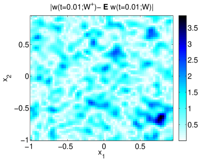
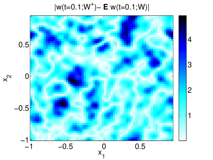
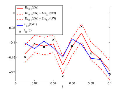
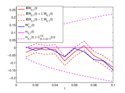
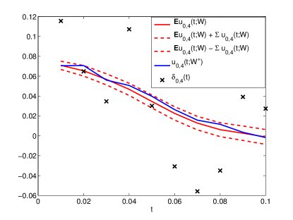
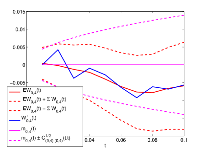
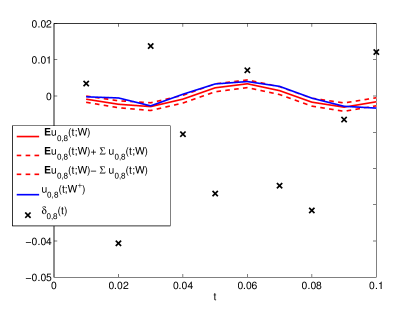
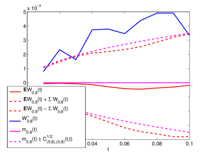
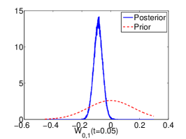
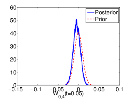
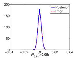
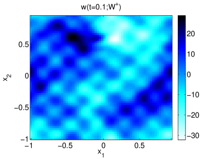
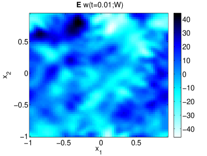
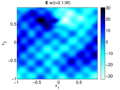
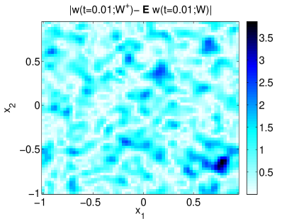
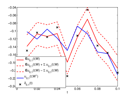
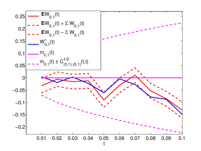
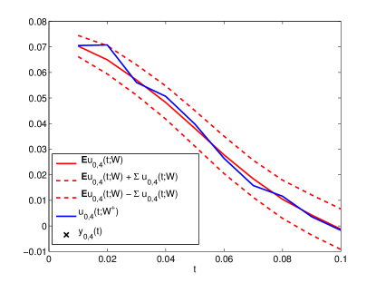
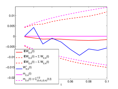
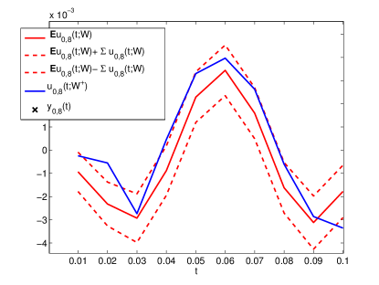
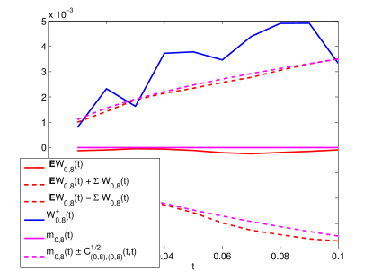
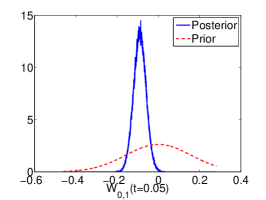
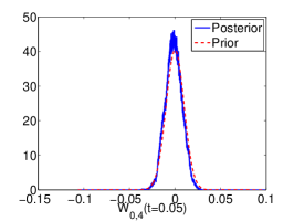
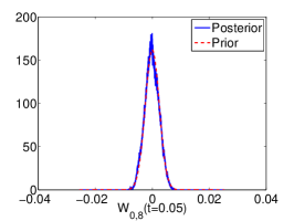
We first consider the observation set-up (i) where pointwise observations of the entire velocity field are made. The true initial and final conditions are plotted in Figure 1, top two panels, for the vorticity field $w$; the middle two panels of Figure 1 show the posterior mean of the same quantities and indicate that the data is fairly informative, since they closely resemble the truth; the bottom two panels of Figure 1 show the absolute difference between the fields in the top and middle panels. The true trajectory, together with the posterior mean and one standard deviation interval around the mean, are plotted in Figure 2, for the wavenumbers $(0,1)$, $(0,4)$, and $(0,8)$, and for both the driving Brownian motion $W$ (right) and the velocity field $u$ (left). This figure indicates that the data is very informative about the $(0,1)$ mode, but less so concerning the $(0,4)$ mode, and there is very little information in the $(0,8)$ mode. In particular for the $(0,8)$ mode the mean and standard deviation exhibit behaviour similar to that under the prior whereas for the $(0,1)$ mode they show considerable improvement over the prior in both position of the mean and width of standard deviations. The posterior on the $(0,4)$ mode has gleaned some information from the data as the mean has shifted considerably from the prior; the variance remains similar to that under the prior, however, so uncertainty in this mode has not been reduced. Figure 3 shows the histograms of the prior and posterior for the same 3 modes as in Fig. 2 at the center time $t=0.05$. One can see here even more clearly that the data is very informative about the $(0,1)$ mode in the left panel, less so but somewhat about the $(0,4)$ mode in the center panel, and it is not informative at all about the $(0,8)$ mode in the right panel.

Figures 4, 5, and 6 are the same as Figures 1, 2, and 3 except for the case of (ii) observation of low Fourier modes. Notice that the difference in the spatial fields are difficult to distinguish by eye, and indeed the relative errors even agree to threshold $10^{-3}$. However, we can see that now the unobserved $(0,4)$ mode in the center panels of Figs. 5 and 6 is not informed by the data and remains distributed approximately like the prior.

Figure 1: Full-field point wise observations. The truth (top), expected value (middle), and absolute distance between them (bottom) of the vorticity $w(t;W)$, for $t=0.01$ (left, relative $L^{2}$ error $e=0.0044$) and $t=0.1$ (right, $e=0.0244$).

Figure 2: Full-field point wise observations. The trajectories $u_{k}(t;W)$ (left) and $W_{k}$ (right), with $k=(0,1)$ (top), $k=(0,4)$ (middle), and $k=(0,8)$ (bottom). Shown are expected values and standard deviation intervals as well as true values. The right hand images also show the expected value and standard deviation of the prior, indicating the decreasing information content of the data for the increasing wave numbers.

Figure 3: Full-field point wise observations. The histograms of the posterior distribution of $W_{k}(t=0.05)$, for $k=(0,1)$ (left), $k=(0,4)$ (middle), and $k=(0,8)$ (right). These plots again illustrate the decreasing information content of the data for the increasing wave numbers.

Figure 4: Observation of Fourier modes $\{\phi_{k}\}_{|k|<4}$. The truth (top), expected value (middle), and absolute distance between them (bottom) of the vorticity $w(t;W)$, for $t=0.01$ (left, relative $L^{2}$ error $e=0.0044$) and $t=0.1$ (right, $e=0.0249$). Notice the similarity to the results of Fig. 1.

Figure 5: Observation of Fourier modes $\{\phi_{k}\}_{|k|<4}$. The trajectories $u_{k}(t;W)$ (left) and $W_{k}$ (right), with $k=(0,1)$ (top), $k=(0,4)$ (middle), and $k=(0,8)$ (bottom). Shown are expected values and standard deviation intervals as well as true values. The right hand images also show the expected value and standard deviation of the prior, indicating the decreasing information content of the data for the increasing wave numbers.

Figure 6: Observation of Fourier modes $\{\phi_{k}\}_{|k|<4}$. The histograms of the posterior distribution of $W_{k}(t=0.05)$, for $k=(0,1)$ (left), $k=(0,4)$ (middle), and $k=(0,8)$ (right). These plots again illustrate the decreasing information content of the data for the increasing wave numbers. Notice the middle panel in which one notices the posterior on $W_{0,4}(t=0.05)$ is much closer to the prior than in Fig. 3.