Universal Doomsday: Analyzing Our Prospects for Survival
Abstract
Given a sufficiently large universe, numerous civilizations almost surely exist. Some of these civilizations will be short-lived and die out relatively early in their development, i.e., before having the chance to spread to other planets. Others will be long-lived, potentially colonizing their galaxy and becoming enormous in size. What fraction of civilizations in the universe are long-lived? The “universal doomsday” argument states that long-lived civilizations must be rare because if they were not, we should find ourselves living in one. Furthermore, because long-lived civilizations are rare, our civilization’s prospects for long-term survival are poor. Here, we develop the formalism required for universal doomsday calculations and show that while the argument has some force, our future is not as gloomy as the traditional doomsday argument would suggest, at least when the number of early existential threats is small.
1 Introduction
The Doomsday Argument [1, 2]111Gott [3] and Nielsen [4] make similar arguments. traditionally runs as follows. Perhaps our civilization will soon succumb to some existential threat (nuclear war, asteroid impact, pandemic, etc.) so that the number of humans ever to exist is not much more than the number who have existed so far. We will call such a civilization short-lived and the total number of humans in it . Alternatively, we might survive all such threats and become long-lived, potentially colonizing other planets and eventually generating a large total number of individuals, . For simplicity we will consider only two possible sizes. We expect . The ratio could easily be as large as a billion.
We don’t know our chances of being short- or long-lived, but we can assign some prior belief or credence and in these two possibilities. These confidence levels should be based on our analysis of specific threats that we have considered and the possibility of other threats of which we are not yet aware.
Suppose that you hold such confidence levels at a time when you don’t know your own position in the entire human race. Now you discover that you are one of the first humans to be born. We will call this datum . If the human race is to be short-lived, is certain. If the human race is to be long-lived, assuming that you can consider yourself a randomly chosen human [5, 6, 7, 8], the chance that you would be in the first is only . Thus you should update your probabilities using Bayes’ Rule, to get
| (1.1) |
Since it is clear that we do face existential threats, is not infinitesimal. Thus , , and doom (our civilization ending soon rather than growing to large size) is nearly certain.
Many counterarguments have been offered (e.g., [9, 10, 11, 7, 12]). The specific issue which will concern us here is the possibility that our universe might contain many civilizations. In that case, we should consider ourselves to be randomly chosen from all individuals in that universe or multiverse. Before taking into account , our chance to be in any given long-lived civilization is then higher than our chance to be in any given short-lived civilization by factor . Taking into account simply cancels this factor, so the chance that we are in a long-lived civilization is just the fraction of civilizations that are long-lived. (More compactly, since each civilization contains individuals who observe , this observation provides no reason to prefer one type of civilization over another.)
Thus if there are many civilizations, the doomsday argument is defeated. However, it returns in another form, called the universal doomsday argument [13, 14]. We are more likely to observe in a universe in which most civilizations are short-lived. While we can no longer conclude anything unique to our own civilization, we can conclude that most civilizations are likely to be short-lived, and thus ours is likely to be short-lived also.
This paper analyzes the universal doomsday argument. In contrast to the traditional doomsday argument, which in almost all circumstances makes doom nearly certain, for many reasonable priors the universal argument gives only a mildly pessimistic conclusion. However, for other priors, the conclusion of the universal argument can be quite strong.
The analysis of many civilizations in the universe can be extended to analyze possible civilizations that might exist according to different theories of the universe. If we take ourselves to be randomly chosen among all observers that might exist [9, 12], the doomsday argument is completely canceled, and after taking into account we find no change in our prior probabilities for different lifetimes of our civilization. This assumption, equivalent to the self-indication assumption [9], is a controversial one, and the authors of the present paper are not in agreement about it. However, for the purpose of the present work we will consider the consequences of denying this idea, and consider ourselves to be randomly chosen only among those individuals who exist in our actual universe.
In the next section we set up the formalism for calculating the probability for a civilization to be long-lived. To simplify the discussion, we focus on a special case where civilizations can have only two possible sizes; the general case is discussed in the Appendix. In Sections 3–6 this formalism is applied to find for several choices of the prior. Our conclusions are summarized and discussed in Section 7.
2 The fraction of long-lived civilizations in the universe
Assume the universe is large enough such that numerous civilizations exist. Assume furthermore that a fraction of the civilizations are long-lived, containing individuals each, and the remaining fraction of the civilizations are short-lived, containing only individuals each. (The general case in which civilizations may have any size, rather than just the specific sizes and , is discussed in the appendix.) We will take the universe to be finite or the problems that arise in infinite universes to have been solved, so that the fraction is well defined.
We do not know what is, but we know it must be in the interval, . We can represent our prior belief, or “best guess” for different values of , with a density function , so that is our prior probability for the fraction of long-lived civilizations to lie within an infinitesimal interval around . We only consider normalized priors so that .
Whatever we take as our prior, we should update it after observing new evidence or data. The rest of this paper is concerned with updating after considering the datum : we were born into a civilization that has not yet reached long-lived status. Bayes’ Rule gives
| (2.1) |
With a given , the probability of observing , , is just the ratio of the number of observers making observation to the total number of observers. Factoring out the total number of civilizations, we divide the number of observers in each civilization finding , which is just , by the average number of observers per civilization, . Thus
| (2.2) |
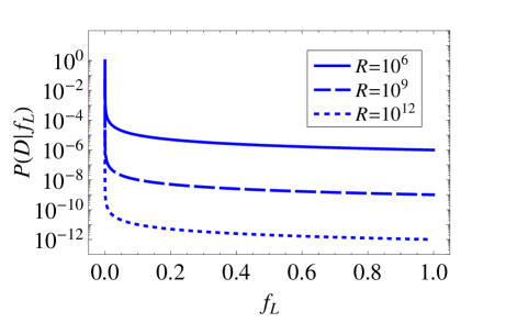
In Fig. 1, we plot the likelihood function given , , and .
Plugging the likelihood into (2.1),
| (2.3) |
The posterior distribution, , expresses our updated belief in different values of after considering that our civilization is not yet long-lived.
Notice that and that is much larger for low values of than for high values of (see Fig. 1). Therefore, when updating our prior, we place more credence in low values of and less credence in high values of , and so become more pessimistic about the fraction of civilizations that reach long-lived status.
We can now compute the probability that our civilization will eventually be long-lived. For any given , this probability is just , the fraction of civilizations that are long-lived. Without considering , we would just take an average of the possible weighted by the prior,
| (2.4) |
To get the posterior chance, we integrate over our posterior probability distribution for ,
| (2.5) |
Given and the prior distribution , (2.5) allows us to determine our civilization’s prospects for long-term survival.
Equation (2.5) is exact, but since we are interested only in , we can always approximate
| (2.6) |
In many cases the contribution from to the numerator is not significant, and we can thus approximate the numerator by , giving
| (2.7) |
In some cases there is a cutoff on that keeps it above and in such cases we can write
| (2.8) |
From (2.8) we can understand the general effect of the universal doomsday argument. The chance that our civilization will survive to large sizes is small when the integral is large. This happens whenever there is a possibility of small where the prior probability of those is large compared to the themselves. So, for example, if our prior gives a collective probability of to a range of near , i.e., we think there’s one chance in a million that only a billionth of all civilizations grow large, then our chance of survival is no more than .
The effect of using (2.7) instead of (2.8) is that the above argument does not apply to below . The doomsday argument is able to increase a prior probability by factor at most, so scenarios with prior probabilities below will never be important.
In the rest of this paper, we will consider several specific priors and see the conclusions to which they lead.
3 The uniform prior
The results for will depend on our prior . Let us start by taking the simplest prior,
| (3.1) |
so that the is equally likely to have any value. This appears to be a reasonable choice of prior when we do not have much quantitative information on the existential threats that we are facing. The posterior density is then
| (3.2) |
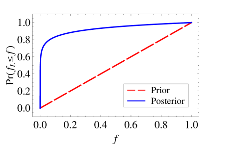
In Fig. 2, we plot the cumulative of the prior and posterior, and , given . Although the probability of low values of increases after considering , the result is not extreme. For example, the probability that is — a low but non-negligible amount.
The probability that our civilization is long-lived, after considering , is
| (3.3) |
Because , our long-term prospects are not too bad. For example, when million, our civilization’s chance of long-term survival is approximately .
We can compare these results with the traditional doomsday argument. Using the uniform prior, the prior chance that our civilization would be long-lived is , and the posterior chance about . If we took a prior chance of survival in the traditional doomsday argument, (1.1) would give our chance of survival as only . Thus, at least in this case, taking account of the existence of multiple civilizations yields a much more optimistic conclusion.
We can reproduce the traditional doomsday argument even in the universal setting, merely by asserting that all civilizations have the same fate, so the benefit of multiple civilizations is eliminated. This would imply giving no credence to any possibilities except (all civilizations short-lived) and (all civilizations long-lived). Thus we could write
| (3.4) |
4 N existential threats
Of course we know that civilizations face more than one existential threat. So let us consider the case where there are statistically independent threats and take a uniform prior for the fraction of civilizations that survive each one. Denote the fraction of civilizations surviving the -th threat . The fraction of civilizations that survive all threats is then
| (4.1) |
and our prior for each threat is
| (4.2) |
so that
| (4.3) |
We can determine the density function for the overall prior, , as follows. Let where . Then
| (4.4) |
Similarly , so is the sum of independent and exponentially distributed random variables, and is thus given by an Erlang (Gamma) distribution,
| (4.5) |
giving
| (4.6) |
The cumulative of the prior, , is shown in Fig. 3(a)
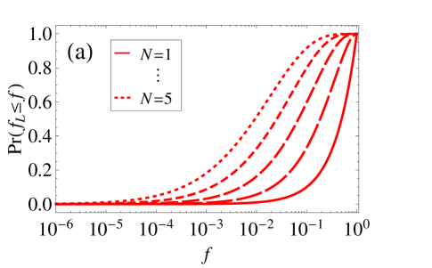
for to . Note that our civilization’s prospects for long-term survival become rather bleak as increases. Even without considering our datum, .
Now, considering our datum , the posterior density is,
| (4.7) |
where is the polylogarithm function, given by
| (4.8) |
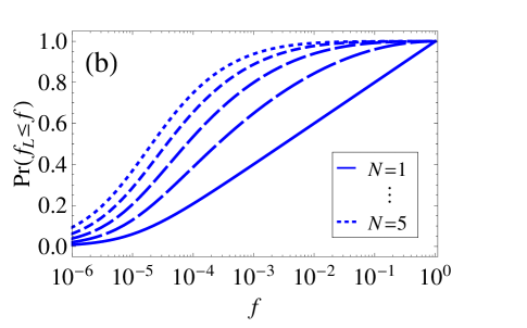
The cumulative of the posterior, , is shown in Fig. 3(b) for to and .
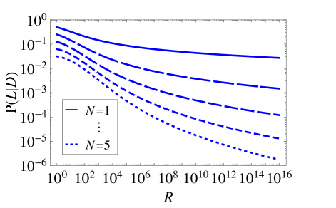
In Fig. 4, is shown as a function of for through .
After considering , our civilization’s prospects for long-term survival are
| (4.9) |
When , we can approximate
| (4.10) |
Notice that when , the prior distribution for is uniform and the results are the same as in the previous section. As seen in Fig. 4, increasing the number of existential threats, , decreases the probability that our civilization will be long-lived. The chance of survival before taking into account is . Updating adds the additional factor
| (4.11) |
which is small whenever . However, only a power of , rather than itself, appears in the denominator, so the effect is more benign than in the traditional doomsday argument of (1.1), so long as is fairly small.
5 An unknown number of threats: Gaussian distribution
It would be foolish to imagine that we know of all existential threats. For example, before the 1930’s no one could have imagined the threat of nuclear war. So there is some uncertainty about the number of threats, . To make a simple model of this effect, let us assume that a fixed fraction of civilizations survive each threat, and thus survive them all. We will take a Gaussian prior for the distribution of ,
| (5.1) |
where
| (5.2) |
For the purposes of the present section it is a good enough approximation to drop the and just use .
The prior expectation value for is
| (5.3) |
The prior chance that our civilization will grow large is
| (5.4) |
providing that , so that the Gaussian does not decline until is already small. Thus the prior chance of survival is quite appreciable.
The posterior chance of survival may be approximated
| (5.5) |
As increases, the numerator in the sum decreases more and more quickly. We can approximate that the denominator decreases by a factor , until , at which point it becomes constant. Thus for , the th term in the sum is larger than the previous term by factor of order
| (5.6) |
so the sum is dominated by terms near or near , whichever is smaller.
In the former case, it is interesting to note that is proportional to , not as one might have thought. The doomsday argument partly cancels the Gaussian suppression of the prior probability, which drops rapidly when .
We can approximate the sum by an integral,
| (5.7) |
so
| (5.8) |
where the last step is for . If is small, this is not too pessimistic a conclusion. For example with threats we find , but for we find .
To be in this regime, we require that , i.e.,
| (5.9) |
for . For this requires , which is not unreasonable.
Fig. 5
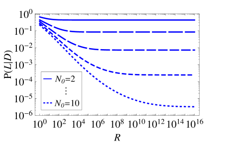
shows our prospects for long-term survival as a function of for various values of . Because , a given corresponds roughly to choosing in the previous section.
Comparing Fig. 5 for each to Fig. 4 for , we see that, as becomes larger, Fig. 4 shows lower survival chances than Fig. 5. In the present case the doomsday argument amplifies the probability of small that arise from a large number of threats, but because we took fixed we don’t consider threats that have very low survival probability. In the previous section, we fixed , but the uniform prior gave some chance to arbitrarily small .
6 An unknown number of threats: exponential distribution
The reason that the conclusion of the previous section was not too pessimistic is that the Gaussian prior for very strongly suppressed numbers of threats . If we take a distribution that falls only exponentially, the result may be quite different. So consider now
| (6.1) |
for some . The prior expectation value for is
| (6.2) |
and the prior chance of survival is
| (6.3) |
The posterior chance of survival is given by
| (6.4) |
If , our prior credence in threats decreases faster than the chance of surviving threats, and the terms in the sum in (6.4) decrease. Except when is very close to , we can ignore and get an optimistic conclusion
| (6.5) |
But if , the situation is different. In this case, our credence in a large number of threats is higher than the survival chance, and then the universal doomsday argument acts to increase our prior for facing many threats and so decrease our expectation of survival. The terms in the sum in (6.4) increase as until we reach some where the existence of begins to matter. This happens when , i.e., when
| (6.6) |
For we can ignore to get in the sum of (6.4). Thus we can split our sum into two parts, which give
| (6.7) |
and so
| (6.8) |
As long as is significantly larger than , this is very small. As an example, we can choose and . This gives the prior probability here, while (5.4) and (5.2) give . While these are nearly the same, (6.8) with gives
| (6.9) |
must lower than from (5.8).
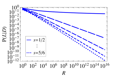
Fig. 6 shows our prospects for long-term survival as a function of for various values of .
7 Summary and discussion
Bayes’ Theorem tells us how the probabilities we assign to various hypotheses should be updated when we learn new information. The Doomsday Argument is concerned with the impact of the important piece of information that we called — that we are among the first humans to be born. Earlier investigations [1, 2, 3, 4, 13, 14] suggested that the resulting probability for our civilization to be long-lived is suppressed by a huge factor , where is the size a civilization may reach if it does not succumb to early existential threats. Here, we attempted a more careful analysis by considering a number of possible choices of prior probabilities. We found that, with a seemingly reasonable choice of the prior, our chances of long-term survival are suppressed by a power of , rather than by , with the power determined by the number of threats . If is not too large, the probability of long-term survival is about a few percent.
This conclusion has been reached by assuming a flat prior distribution, , for the fraction of civilizations surviving statistically independent threats (labeled by ). This appears to be a reasonable assumption, reflecting our present state of ignorance on the subject. We also considered a prior where the survival probability for each threat is a fixed number , while the number of threats is a stochastic variable with a Gaussian distribution of width . Once again, we find, assuming that is not too small and is not too large, that the Bayesian suppression factor is much smaller than suggested by the naive Doomsday Argument.
In our analysis, we adopted a model where civilizations can have only two possible sizes, and . This model is of course not realistic in detail, but it may well capture the bimodal character of the realistic size distribution. Civilizations that actively engage in colonizing other planetary systems and reach a certain critical size are likely to grow extremely large, while civilizations confined to their home planet must be rather limited in size.
Even though we found a greater survival probability than in Refs. [1, 2, 3, 4, 13, 14], our conclusions can hardly be called optimistic. With the priors that we considered, the fraction of civilizations that last long enough to become large is not likely to exceed a few percent. If there is a message here for our own civilization, it is that it would be wise to devote considerable resources (i) for developing methods of diverting known existential threats and (ii) for space exploration and colonization. Civilizations that adopt this policy are more likely to be among the lucky few that beat the odds. Somewhat encouragingly, our results indicate that the odds are not as overwhelmingly low as suggested by earlier work.
Appendix A Arbitrary possibilities for civilization size
In this appendix we give a formalism for considering all possible civilization sizes. Let a scenario be a set of numbers , giving the fraction of civilizations that have each size . Since every civilization has some size, we must have . We will write for the entire vector of numbers . The average number of observers per civilization in scenario is
| (A.1) |
which we will assume is finite.
Now let denote the prior probability that we assign to each possible scenario . The probabilities must be normalized,
| (A.2) |
where
| (A.3) |
We suppose that already contains a term such as that excludes unnormalized .
Let denote the size of our civilization. We will not be concerned here with issues related to civilizations with fewer than observers, so let us suppose that is supported only when for . Now we consider the datum , that we are in the first individuals in our civilization. The chance for a randomly chosen observer to observe is
| (A.4) |
Now let be some property of , such as the average size of a civilization or the chance that the civilization has more than a certain number of members. The average value of not taking into account is
| (A.5) |
Now we take into account using Bayes’ Rule. We find
| (A.6) |
which is the arbitrary-size generalization of (2.3). The average value of taking into account is
| (A.7) |
A particularly simple case is when . The expected value of the total size of our civilization taking into account is
| (A.8) |
Alternatively, let be the fraction of civilizations in scenario that grow larger than some threshold . The posterior chance that our civilization will reach this threshold is then
| (A.9) |
This is just the fraction of large civilizations in the different scenarios, weighted by prior probability of the scenario and the inverse of the average civilization size according to that scenario.
Unfortunately, the set of possible priors is so large here that it is difficult to make any progress. It seems likely to us that civilizations will either remain confined to a single planet and eventually be wiped out by some disaster, or spread through the galaxy and grow to large size. We can approximate this by considering supported only at two sizes and ,
| (A.10) |
where we have written for and for . Then we recover the results in the main text. Integrals become , is just , is , (A.6) becomes (2.3), and (A.9) becomes (2.5).
References
- [1] B. Carter unpublished.
- [2] J. Leslie, Risking the world’s end, Bulletin of the Canadian Nuclear Society May 1989 (1989) 10–15.
- [3] J. R. Gott, III, Implications of the copernican principle for our future prospects, Nature 363 (1993) 315–319.
- [4] H. B. Nielsen, Random dynamics and relations between the number of fermion generations and the fine structure constants, Acta Physica Polonica B 20 (1989) 427–468.
- [5] A. Vilenkin, Predictions from quantum cosmology, Phys. Rev. Lett. 74 (1995) 846–849, [gr-qc/9406010].
- [6] D. N. Page, Sensible quantum mechanics: are probabilities only in the mind?, Int.J.Mod.Phys. D5 (1996) 583–596, [gr-qc/9507024].
- [7] N. Bostrom, Anthropic Bias: Observation Selection Effects. Routledge, New York, 2002.
- [8] J. Garriga and A. Vilenkin, Prediction and explanation in the multiverse, Phys.Rev. D77 (2008) 043526, [arXiv:0711.2559].
- [9] D. Dieks, Doomsday — or: The dangers of statistics, Philosophical Quarterly 42 (1992) 78–84.
- [10] T. Kopf, P. Krtous, and D. N. Page, “Too soon for doom gloom.” Physics preprint ALBERTA-THY-17-94, http://arXiv.org/abs/gr-qc/9407002.
- [11] P. Bartha and C. Hitchcock, No one knows the date or the hour: An unorthodox application of Rev. Bayes’s theorem, Philosophy of Science (Proceedings) 66 (1999) S339–S353.
- [12] K. D. Olum, The Doomsday argument and the number of possible observers, Phil.Q. 52 (2002) 164, [gr-qc/0009081].
- [13] J. Knobe, K. D. Olum, and A. Vilenkin, Philosophical implications of inflationary cosmology, Brit.J.Phil.Sci. 57 (2006) 47–67, [physics/0302071].
- [14] A. Gerig, The Doomsday Argument in Many Worlds, arXiv:1209.6251.