A Monte Carlo Code for Relativistic Radiation Transport Around Kerr Black Holes

Abstract

We present a new code for radiation transport around Kerr black holes, including arbitrary emission and absorption mechanisms, as well as electron scattering and polarization. The code is particularly useful for analyzing accretion flows made up of optically thick disks and optically thin coronae. We give a detailed description of the methods employed in the code, and also present results from a number of numerical tests to assess its accuracy and convergence.

1 INTRODUCTION

Since the beginning of X-ray astronomy over 50 years ago, there has been steadily growing interest in relativistic radiation transport. Because of the high energies of both photons and electrons relevant to these astrophysical sources, special relativistic effects must be included in most particle interactions. And because the central engines of so many X-ray sources are compact objects such as neutron stars and black holes, full general relativity must also be incorporated into any physically realistic code.

Here we present in detail for the first time the fully relativistic Monte Carlo radiation transport code Pandurata. While this is the first formal description of the code in the literature, it has been under development for many years and has already been used in numerous publications (Schnittman & Krolik, 2009, 2010; Noble et al., 2011; Schnittman et al., 2012). Pandurata  shares features with numerous existing codes in the literature, but we believe its combination of full general relativity, wide range of emission and absorption processes, scattering, polarization, and optically thin/thick capabilities make it uniquely valuable in the rapidly evolving field of black hole astrophysics. Most recently, in Schnittman et al. (2012) we have demonstrated how the code may be used to take a major step towards bridging the gap between global magneto-hydrodynamics (MHD) simulations and real X-ray observations of accreting black holes.

The literature of radiation transport in astrophysics is extremely broad and includes scores of different techniques and applications. It would be a futile endeavor to attempt to give a comprehensive summary of work here. Rather, we will simply highlight a few recent contributions that are most relevant to the applications of interest, namely photon transport around Kerr black holes. By far the most common approach has been ray-tracing geodesic paths backwards from a distant observer to the accretion flow, calculating a transfer function of some sort, and coupling this to some model for emission to generate spectra and light curves. A few of the many examples of this observer-to-emitter approach include Rauch & Blandford (1994); Broderick & Blandford (2003, 2004); Schnittman & Bertschinger (2004); Dovciak et al. (2004); Schnittman et al. (2006); Noble et al. (2007); Dexter & Agol (2009); Dexter et al. (2009).

A smaller number of codes have been written with the emitter-to-observer approach, which may be more physically intuitive, but is almost always more computationally intensive. With the exception of Laor et al. (1990); Laor (1991); Kojima (1991), which use uniform sampling of emission angles, these codes are generally Monte Carlo in nature, such as grmonty by Dolence et al. (2009), and the present work. As we will show below, particularly when electron scattering is included, the emitter-to-observer paradigm is almost essential for capturing the most relevant physics of the problem.

Another feature that is relatively uncommon in these ray-tracing codes, but of increasing interest in the high energy community, is polarization. It is included in Agol & Krolik (2000); Dovciak et al. (2008); Huang et al. (2009); Shcherbakov & Huang (2011); Huang & Shcherbakov (2011); Marin et al. (2012), although often only for vacuum transport and not including scattering. Disk polarization is treated by Laor et al. (1990); Matt et al. (1993); Dovciak et al. (2008) for both Schwarzschild and Kerr black holes, but neglecting electron scattering. Dovciak et al. (2011) includes illumination from a source above the disk, while Dovciak et al. (2008) includes a cold plane-parallel atmosphere above the disk, geometrically thin with varying optical depth. A small number of ray-tracing codes also allow for non-standard black hole metrics as a way of testing general relativity. Krawczynski (2012) follows the emitter-to-observer paradigm for calculating polarized flux from a thermal disk, and Psaltis & Johannsen (2012) describes an observer-to-emitter framework that can be applied to a large number of space-time tests such as timing, spectra, and imaging (Johannsen & Psaltis, 2010a, b, 2011, 2012).

The body of literature including detailed scattering and polarization is generally restricted to flat spacetime, and often only the most simple geometries (Connors & Stark, 1977; Connors et al., 1980; Sunyaev & Titarchuk, 1985; Haardt & Maraschi, 1993; Haardt et al., 1994; Poutanen & Svensson, 1996). Here we attempt to synthesize the strengths of all these various codes into a single flexible radiation transport tool for analyzing both global MHD simulations, and also simpler toy accretion models. The ultimate goal is to produce concrete predictions that can be compared directly with the large and continually growing body of X-ray observations of accreting black holes.

Precisely because of the large interest in this topic, we give here a comprehensive description of the technical components of our radiation transport code Pandurata. We hope that the techniques outlined below will be valuable to others who are interested in developing similar (or even better, more powerful) tools. We also present the results from a suite of simple numerical tests to verify the code, thus lending support and increasing our confidence in earlier work based on Pandurata.

2 LOCAL ORTHONORMAL FRAMES

The most general input for Pandurata  is a body of tabulated data including the extrinsic fluid variables density, temperature, magnetic field, and the 4-velocity at each point in a three-dimensional volume. Multiple data slices in the time coordinate allow for studies of variability. The coordinates are Boyer-Lindquist for a Kerr BH with mass $M$ and dimensionless spin parameter $a/M$. The fluid variables are given in physical cgs units for a specific BH mass and accretion rate. The source of the data is quite general, and Pandurata  has been used successfully to analyse simulation data from the relativistic MHD codes Harm3D  (Noble et al., 2011; Schnittman et al., 2012) and GRMHD  (Schnittman et al., 2006), as well as 2D hydro simulations (Schnittman & Rezzolla, 2006) and analytic models for the accretion disk and corona (Schnittman & Krolik, 2009, 2010).

We adopt a $(-+++)$ metric signature, and convention where Greek indices run from 0 to 3, and Latin indices are restricted to spatial coordinates 1 to 3. The coordinate metric is given by (Boyer & Lindquist, 1967):

$$g_{\mu\nu}=\begin{pmatrix}-\alpha^{2}+\omega^{2}\varpi^{2}&0&0&-\omega\varpi^{2}\\ 0&\rho^{2}/\Delta&0&0\\ 0&0&\rho^{2}&0\\ -\omega\varpi^{2}&0&0&\varpi^{2}\end{pmatrix}\,.$$ (1)

This allows for a relatively simple form for the inverse metric:

$$g^{\mu\nu}=\begin{pmatrix}-1/\alpha^{2}&0&0&-\omega/\alpha^{2}\\ 0&\Delta/\rho^{2}&0&0\\ 0&0&1/\rho^{2}&0\\ -\omega/\alpha^{2}&0&0&1/\varpi^{2}-\omega^{2}/\alpha^{2}\end{pmatrix}\,.$$ (2)

In geometrized units with $G=c=1$, we have

$$\rho^{2} \equiv r^{2}+a^{2}\cos^{2}\theta$$ (3a)

$$\Delta \equiv r^{2}-2Mr+a^{2}$$ (3b)

$$\alpha^{2} \equiv \frac{\rho^{2}\Delta}{\rho^{2}\Delta+2Mr(a^{2}+r^{2})}$$ (3c)

$$\omega \equiv \frac{2Mra}{\rho^{2}\Delta+2Mr(a^{2}+r^{2})}$$ (3d)

$$\varpi^{2} \equiv \left[\frac{\rho^{2}\Delta+2Mr(a^{2}+r^{2})}{\rho^{2}}\right]\sin^{2}\theta\,.$$ (3e)

2.1 Simulation Data

We briefly describe here the format of data from the Harm3D  MHD simulations. Similar data can be generated from GRMHD, and any analytic model can be understood as a subset of the full tabulated simulation data. As described in greater detail in Noble et al. (2011) and Schnittman et al. (2012), the first step in post-processing the simulation data is to convert from code units of density and local dissipation to cgs units of density and temperature. Given the density everywhere, we integrate the optical depth along paths of constant $(r,\phi)$ coordinates starting from both $\theta=0$ and $\theta=\pi$ to get $\tau_{\rm top}(r,\theta,\phi)$ and $\tau_{\rm bot}(r,\theta,\phi)$. The disk midplane can then be defined as the surface $\theta_{\rm mid}(r,\phi)$ where $\tau_{\rm top}(r,\theta_{\rm mid},\phi)=\tau_{\rm bot}(r,\theta_{\rm mid},\phi)$. When $\tau(r,\theta_{\rm mid},\phi)>1$, the disk is optically thick and we define a top and bottom photosphere $\Theta(r,\phi)$ such that $\tau_{\rm top}(r,\Theta_{\rm top},\phi)=\tau_{\rm bot}(r,\Theta_{\rm bot},\phi)=1$. In Figure 1 we show a slice in the $(r,z)$ plane of simulation data from the Harm3D  “ThinHR” run (Noble et al., 2010). The local temperature is represented by the logarithmic color scale, and the contours show surfaces of constant $\tau$. In Figure 2 we show a three-dimensional representation of the photosphere surface $\Theta_{\rm top}(r,\phi)$ for the same simulation data.

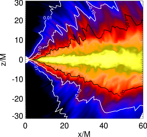
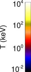
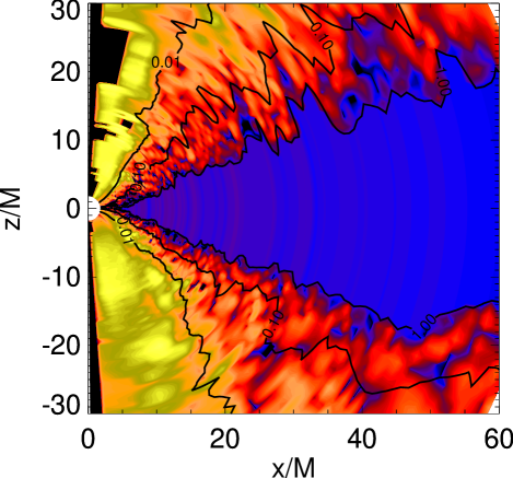
Figure 1: Fluid density (top) and temperature (bottom) profile for a slice of Harm3D  data in the $(r,z)$ plane, taken from the ThinHR simulation (Noble et al., 2010, 2011). Contours show surfaces of constant optical depth with $\tau=0.01,0.1,1.0$. Fiducial values for the black hole mass $M=10M_{\odot}$ and luminosity $L=0.1L_{\rm Edd}$ were used, as described in Schnittman et al. (2012).

From the photosphere surfaces, thermal photon are launched into the optically thin corona above and below the disk. Because the opacity within the disk is usually dominated by electron scattering, the seed photons are emitted with the limb-darkening and polarization dependence on angle given by Chandrasekhar (1960). The spectrum is that of a diluted blackbody with temperature $T_{\rm eff}$ and hardening factor $f$:

$$I_{\nu}=\frac{1}{f^{4}}B_{\nu}(f\,T_{\rm eff}),$$ (4)

with $B_{\nu}$ the black-body function. We take $f=1.8$ (Shimura & Takahara, 1995) and the local effective temperature is given by

$$T_{\rm eff}(r,\phi)\equiv\left(\frac{\mathcal{F}(r,\phi)}{\sigma}\right)^{1/4},$$ (5)

where $2\mathcal{F}(r,\phi)$ is the total integrated luminosity in the optically thick part of the disk (the factor of 2 comes from the fact that the flux is emitted equally from the top and bottom photospheres). As shown in Figure 1, the gas has a constant temperature inside the disk for a given $(r,\phi)$, due to the high level of thermalization caused by the large optical depth.

Synchrotron and bremsstrahlung seed photons can also be generated in the coronal regions, in which case we use an unpolarized, isotropic distribution function for the emission angles, as measured in the local fluid frame. Due to the high temperatures and low densities of the coronal regions, the net power in the coronal seed photons is typically much lower than that of inverse-Compton scattering from the thermal seeds coming from the disk (Schnittman et al., 2012).

2.2 Photosphere tetrads

We begin with a short discussion of notation. As stressed in Misner et al. (1973), vectors are invariant geometric objects independent of coordinate system, and we represent them with bold font $\mathbf{u}$, while the components in a specific basis are represented with italics: $u^{\mu}$. We adopt a naming convention such that the components of a vector in the coordinate basis are represented by $\mu$ and in the local fluid frame by $\hat{\mu}$. The basis vectors themselves are labeled with $(\mu)$. For example, the coordinate basis is spanned by the vectors $\mathbf{e}_{(\mu)}$ with components $e_{(\mu)}^{\nu}=\delta_{(\mu)}^{\nu}$, where $\delta$ is the usual Kronneker delta. Note that the coordinate basis vectors are not normalized, and not even orthogonal in the Kerr metric:

$$\mathbf{e}_{(\mu)}\cdot\mathbf{e}_{(\nu)}=g_{\alpha\beta}e_{(\mu)}^{\alpha}e_{(\nu)}^{\beta}=g_{\mu\nu}\,.$$ (6)

Einstein’s Equivalence Principle, one of the bedrocks of general relativity, states that an orthonomal basis (a “tetrad”) can be defined at any point in space. In fact, an arbitrary number of tetrads can be defined at any point, and are all related by Lorentz boosts and/or rotations. One particularly useful tetrad in the Kerr metric is that of the zero-angular-momentum observer (ZAMO; Bardeen et al. (1972)). We denote the ZAMO frame with $\tilde{\mu}$ labels. It can be constructed from the coordinate basis by:

$$\mathbf{e}_{(\tilde{t})} = \frac{1}{\alpha}\mathbf{e}_{(t)}+\frac{\omega}{\alpha}\mathbf{e}_{(\phi)}$$ (7a)

$$\mathbf{e}_{(\tilde{r})} = \sqrt{\frac{\Delta}{\rho^{2}}}\mathbf{e}_{(r)}$$ (7b)

$$\mathbf{e}_{(\tilde{\theta})} = \sqrt{\frac{1}{\rho^{2}}}\mathbf{e}_{(\theta)}$$ (7c)

$$\mathbf{e}_{(\tilde{\phi})} = \sqrt{\frac{1}{\varpi^{2}}}\mathbf{e}_{(\phi)}\,.$$ (7d)

Any vector can be represented by its components in different bases:

$$\mathbf{u}=\mathbf{e}_{(\mu)}u^{\mu}=\mathbf{e}_{(\tilde{\mu})}u^{\tilde{\mu}}\,,$$ (8)

and the components are related by a linear transformation $E_{\,\,\tilde{\mu}}^{\mu}$:

$$u^{\mu} = E_{\,\,\tilde{\mu}}^{\mu}u^{\tilde{\mu}}\,,$$ (9a)

$$u^{\tilde{\mu}} = [E^{-1}]_{\,\,\mu}^{\tilde{\mu}}u^{\mu}\,.$$ (9b)

In our example of the ZAMO frame, $E_{\,\,\tilde{\mu}}^{\mu}$ is given by

$$E_{\,\,\tilde{\mu}}^{\mu}=\begin{pmatrix}\frac{1}{\alpha}&0&0&0\\ 0&\sqrt{\frac{\Delta}{\rho^{2}}}&0&0\\ 0&0&\frac{1}{\rho}&0\\ \frac{\omega}{\alpha}&0&0&\frac{1}{\varpi}\end{pmatrix}\,.$$ (10)

At each point on the photosphere we define a tetrad in the comoving fluid frame (designated with sub/superscripts $\hat{\mu}$) such that the time coordinate is in the direction of the fluid 4-velocity:

$$e_{(\hat{t})}^{\mu}=u^{\mu}.$$ (11)

In our notation, this equation says that the 4-vector tangent to the world line of an observer moving with the fluid can be expressed in the Boyer-Lindquist coordinate basis with components $\mu$, or in the local frame with components $\hat{\mu}$ with $e_{(\hat{t})}^{\hat{\mu}}=[1,0,0,0]$. The spatial basis vectors in the fluid frame $e_{(\hat{i})}^{\mu}$ are constucted via a method similar to Beckwith et al. (2008), including a slight modification to ensure the right-handedness of the basis such that $\mathbf{e}_{(\hat{z})}$ is in the $-\theta$ direction. For completeness, we reproduce those definitions here:

$$C_{0} = u_{\phi}/u_{t}\,,$$ (12a)

$$C_{1} = \frac{u^{r}}{u^{t}+C_{0}u^{\phi}}\,,$$ (12b)

$$C_{2} = \frac{g^{tt}+2C_{0}g^{t\phi}+C_{0}^{2}g^{\phi\phi}}{g^{rr}}\,,$$ (12c)

$$C_{3} = u^{t}+C_{1}C_{2}u^{r}+C_{0}u^{\phi}\,,$$ (12d)

$$N_{1} = \sqrt{g_{tt}C_{0}^{2}-2g_{t\phi}C_{0}+g_{\phi\phi}}\,,$$ (12e)

$$N_{2} = \sqrt{g^{tt}C_{1}^{2}+2g^{t\phi}C_{1}^{2}C_{0}+g^{rr}+g^{\phi\phi}C_{0}^{2}C_{1}^{2}}\,,$$ (12f)

$$N_{3} = \sqrt{(u^{\theta})^{2}(g^{tt}+2g^{t\phi}C_{0}+g^{rr}C_{1}^{2}C_{2}^{2}+g^{\phi\phi}C_{0}^{2})+g^{\theta\theta}C_{3}^{2}}\,,$$ (12g)

and

$$e_{(\hat{x})}^{\mu} = \left[-\frac{1}{N_{2}}(g^{tt}C_{1}+g^{t\phi}C_{0}C_{1}),\frac{g^{rr}}{N_{2}},0,-\frac{1}{N_{2}}(g^{t\phi}C_{1}+g^{\phi\phi}C_{0}C_{1})\right]\,,$$ (13a)

$$e_{(\hat{y})}^{\mu} = \left[-\frac{C_{0}}{N_{1}},0,0,\frac{1}{N_{1}}\right]\,,$$ (13b)

$$e_{(\hat{z})}^{\mu} = \left[\frac{1}{N_{3}}(g^{tt}u^{\theta}+g^{t\phi}C_{0}u^{\theta}),\frac{g^{rr}C_{1}C_{2}u^{\theta}}{N_{3}},-\frac{g^{\theta\theta}C_{3}}{N_{3}},\frac{1}{N_{3}}(g^{t\phi}u^{\theta}+g^{\phi\phi}C_{0}u^{\theta})\right]\,.$$ (13c)

From this tetrad basis, any other tetrad in the fluid frame can be constructed from a simple rotation of the spatial basis vectors. We take as our preferred basis (now labeled with $\mathbf{e}_{(\bar{\mu})}$) one in which $\mathbf{e}_{(\bar{z})}$ is normal to the photosphere surface. Whether we are using simulation data or an analytic model for the disk surface, the photosphere is described by a two-dimensional surface on the top and bottom of the disk: $\Theta_{\rm top}(r,\phi)$ and $\Theta_{\rm bot}(r,\phi)$. From these functions, at each point on the photosphere we can construct two vectors tangent to the disk surface through the following process. Start with the coordinate-based vectors

$$dr^{\mu}=[0,\Delta r,\frac{\partial\Theta}{\partial r}\Delta r,0]$$ (14a)

and

$$d\phi^{\mu}=[0,0,\frac{\partial\Theta}{\partial\phi}\Delta\phi,\Delta\phi]\,,$$ (14b)

where $\Delta r$ and $\Delta\phi$ are the differential sizes of the fluid cell in question. Next, subtract off the components parallel to $\mathbf{e}_{(\hat{t})}$:

$$\mathbf{dr}^{\prime}=\mathbf{dr}-(\mathbf{dr}\cdot\mathbf{e}_{(\hat{t})})\mathbf{e}_{(\hat{t})}$$ (15a)

and

$$\mathbf{d}\bm{\phi}^{\prime}=\mathbf{d}\bm{\phi}-\mathbf{d}\bm{\phi}\cdot\mathbf{e}_{(\hat{t})})\mathbf{e}_{(\hat{t})}\,.$$ (15b)

When $\mathbf{dr}^{\prime}$ and $\mathbf{d}\bm{\phi}^{\prime}$ are projected into the fluid frame, they will have only spatial components and will be tangent to the photosphere. In this basis, we can easily construct the normal vector by taking the 3-vector cross product:

$$dz^{\hat{k}}=\epsilon_{\,\,\hat{i}\hat{j}}^{\hat{k}}dr^{\prime\hat{i}}d\phi^{\prime\hat{j}}\,.$$ (16)

This procedure has the added advantage of giving the proper area of the photosphere patch subtended by the vectors $\mathbf{dr}^{\prime}$ and $\mathbf{d}\bm{\phi}^{\prime}$ by $dA=|\mathbf{dz}|$. This formula for $dA$ will be helpful for determining the amplitude of emitted flux from each patch of the disk, since the emission function is typically defined in the local fluid frame. Because $\mathbf{dr}^{\prime}$ and $\mathbf{d}\bm{\phi}^{\prime}$ are not generally orthogonal, we also define the $\mathbf{dx}$ and $\mathbf{dy}$ tangent vectors by $\mathbf{dx}=\mathbf{dr}^{\prime}$, $dy^{\hat{t}}=0$ and

$$dy^{\hat{k}}=\epsilon_{\,\,\hat{i}\hat{j}}^{\hat{k}}dz^{\hat{i}}dx^{\hat{j}}\,.$$ (17)

Figure 2: Three-dimensional representation of the disk photosphere surface $\Theta_{\rm top}(r,\phi)$, along with the local spatial tetrad definitions of equation (18a). The simulation data is the same as in Figure 1. The color scale is a linear representation of the disk’s local thermal temperature. The labels $(r_{i},\phi_{j})$ correspond to coordinates of the computational grid boundaries.

To complete the tetrad, we simply need to normalize the differential basis vectors. Returning to the coordinate basis, we have:

$$e^{\mu}_{(\bar{t})} = e^{\mu}_{(\hat{t})}=u^{\mu}$$ (18a)

$$e^{\mu}_{(\bar{x})} = dx^{\mu}/(g_{\alpha\beta}dx^{\alpha}dx^{\beta})^{1/2}$$ (18b)

$$e^{\mu}_{(\bar{y})} = \pm dy^{\mu}/(g_{\alpha\beta}dy^{\alpha}dy^{\beta})^{1/2}$$ (18c)

$$e^{\mu}_{(\bar{z})} = \pm dz^{\mu}/(g_{\alpha\beta}dz^{\alpha}dz^{\beta})^{1/2}\,.$$ (18d)

The $\pm$ in the definitions for $\mathbf{e}_{(\bar{y})}$ and $\mathbf{e}_{(\bar{z})}$ are chosen for the top $(+)$ and bottom $(-)$ photosphere surfaces so that the spatial basis vectors are oriented in a right-hand fashion and to ensure that $\mathbf{e}_{(\bar{z})}$ points away from the disk body. In Figure 2 we show how these tetrad basis vectors are oriented on the photosphere surface.

2.3 Coronal tetrads

In addition to launching photons from the disk surface, we often want the option of including seeds from within the corona, due to thermal bremsstrahlung, cyclo-synchrotron, or other radiation processes. Analogous with the comoving surface element defined above for disk emission, for coronal emission we need to define a volume element and associated tetrad at each point in the simulation space. Like the tetrads defined above, the time axis is defined along the local fluid 4-velocity $u^{\mu}$. However, unlike the surface tetrads, the volume tetrads have no preferred orientation, so we can simply use the spatial coordinate vectors projected onto the space orthogonal to $u^{\mu}$:

$$dr^{\mu} = [0,\Delta r,0,0]\,,$$ (19a)

$$d\theta^{\mu} = [0,0,\Delta\theta,0]\,,$$ (19b)

$$d\phi^{\mu} = [0,0,0,\Delta\phi]\,,$$ (19c)

$$\mathbf{dr}^{\prime} = \mathbf{dr}-(\mathbf{dr}\cdot\mathbf{e}_{(\hat{t})})\,,$$ (20a)

$$\mathbf{d}\bm{\theta}^{\prime} = \mathbf{d}\bm{\theta}-(\mathbf{d}\bm{\theta}\cdot\mathbf{e}_{(\hat{t})})\,,$$ (20b)

$$\mathbf{d}\bm{\phi}^{\prime} = \mathbf{d}\bm{\phi}-(\mathbf{d}\bm{\phi}\cdot\mathbf{e}_{(\hat{t})})\,.$$ (20c)

The proper volume element subtended by these vectors is given by the 3-vector triple product in the local fluid frame. While there is no real preferred orientation for the spatial axes, we still need to go through the process of defining some orthonormal basis to project the above vectors and thereby calculate vector products. In practice, we set $\mathbf{e}_{(\hat{x})}$ along the $\mathbf{dr}^{\prime}$ direction:

$$dx^{\mu}=dr^{\prime\mu},$$ (21a)

then set the y-axis roughly along the $$\phi$$ coordinate direction

$$dy^{\hat{k}}=\epsilon_{\,\,\hat{i}\hat{j}}^{\hat{k}}dx^{{}^{\prime}\hat{i}}d\theta^{\hat{j}}\,,$$ (21b)

and the z-axis normal to both:

$$dz^{\hat{k}}=\epsilon_{\,\,\hat{i}\hat{j}}^{\hat{k}}dx^{{}^{\prime}\hat{i}}dy^{\hat{j}}\,.$$ (21c)

As above for the photosphere tetrads, the final step is to normalize all the basis vectors:

$$e^{\mu}_{(\bar{t})} = e^{\mu}_{(\hat{t})}=u^{\mu}$$ (22a)

$$e^{\mu}_{(\bar{x})} = dx^{\mu}/(g_{\alpha\beta}dx^{\alpha}dx^{\beta})^{1/2}$$ (22b)

$$e^{\mu}_{(\bar{y})} = dy^{\mu}/(g_{\alpha\beta}dy^{\alpha}dy^{\beta})^{1/2}$$ (22c)

$$e^{\mu}_{(\bar{z})} = dz^{\mu}/(g_{\alpha\beta}dz^{\alpha}dz^{\beta})^{1/2}\,.$$ (22d)

Unlike the photosphere case, since there is no “top” or “bottom” in the corona, we need not be concerned about the orientation of the $\mathbf{e}_{(\bar{z})}$ vector, and simply require a right-handed (x,y,z) convention.

3 RAY-TRACING

3.1 Geodesics

The ray-tracing portion of Pandurata  integrates the geodesic trajectories of photons in the Kerr metric. From the tetrad frames defined in the previous section, the initial direction of a photon is selected from an isotropic distribution in the emitting fluid frame (limited to a hemisphere in the case of an optically thick photosphere surface).

The geodesic integrater is the same as that described in Schnittman & Bertschinger (2004), based on a Hamiltonian approach. Because the Kerr metric is stationary, the momentum conjugate to the time coordinate $t$ is conserved, and corresponds to the (negative) specific energy of a particle ($m^{2}=1$) or photon ($m^{2}=0$). We can replace the affine parameter with the coordinate time and write the Hamiltonian as

$$H(x^{i},p_{i})\equiv-p_{0}=\frac{g^{0i}p_{i}}{g^{00}}+\left[\frac{g^{ij}p_{i}p_{j}+m^{2}}{-g^{00}}+\left(\frac{g^{0i}p_{i}}{g^{00}}\right)^{2}\right]^{1/2}\,,$$ (23)

with equations of motion

$$\frac{dx^{i}}{dt}=\frac{\partial H_{1}}{\partial p_{i}}\,,$$ (24a)

$$\frac{dp_{i}}{dt}=-\frac{\partial H_{1}}{\partial x^{i}}\,.$$ (24b)

In Boyer-Lindquist coordinates, the Hamiltonian can be written thus:

$$H(r,\theta,\phi,p_{r},p_{\theta},p_{\phi})=\omega p_{\phi}+\alpha\left(\frac{\Delta}{\rho^{2}}p_{r}^{2}+\frac{1}{\rho^{2}}p_{\theta}^{2}+\frac{1}{\varpi^{2}}p_{\phi}^{2}+m^{2}\right)^{1/2}\,,$$ (25)

using the same notation defined above in equations (3a-3e). Because the metric, and thus Hamiltonian, is axisymmetric, $p_{\phi}$ is also an integral of the motion. We are thus left with five coupled first-order ordinary differential equations for $(r,\theta,\phi,p_{r},p_{\theta})$. The third integral of motion, Carter’s constant (Carter, 1968)

$$\mathcal{Q}\equiv p_{\theta}^{2}+\cos^{2}\theta\left[a^{2}(m^{2}-p_{0}^{2})+p_{\phi}^{2}/\sin^{2}\theta\right],$$ (26)

is used as an independent check of the accuracy of the numerical integration.

Figure 3: Convergence of the geodesic integrator, as determined by the accuracy of the conserved quantity $\mathcal{Q}$. As expected, we find 5^th-order convergence for the Cash-Karp adaptive time step integrator.

For the numerical integration of geodesics, we use a 5^th-order Cash-Karp algorithm with adaptive step size (Press et al., 1992). In Figure 3 we show the accuracy of the integrator by plotting the average deviation in the Carter constant for a selection of photons around a black hole with $a/M=0.99$, as a function of step segments. We typically set the tolerance at $10^{-8}$ per step, which we find allows sufficient sampling of the fluid variables near the black hole. Because of the frequent table look-ups required when using simulation data, there is little to be gained by using more advanced integration techniques such as Bulirsch-Stoer or the semi-analytic approaches of Rauch & Blandford (1994) or Dexter & Agol (2009) that calculate the geodesic endpoint in a single integral evaluation, and are more appropriate for vacuum transport.

3.2 Polarization

Pandurata  is also capable of polarized transport along geodesics. The polarization vector is a space-like vector normal to the photon direction. For a photon with wavevector $\mathbf{k}$, the polarization vector $\mathbf{f}$ is constrained by $\mathbf{f}\cdot\mathbf{f}=1$ and $\mathbf{f}\cdot\mathbf{k}=0$ (Connors et al., 1980). The vector $\mathbf{f}$ is parallel transported along the geodesic path: $\nabla_{\mathbf{k}}\mathbf{f}=0$, but instead of explicitly solving the parallel transport equation, we can take advantage of the complex-valued Walker-Penrose constant $\kappa_{\rm wp}$ (Walker & Penrose, 1970; Connors & Stark, 1977).

After solving for the wavevector $k^{\mu}$ along the geodesic path, $\kappa_{\rm wp}$ is given at any point by

$$\kappa_{\rm wp} = \left[(k^{t}f^{r}-k^{r}f^{t})+a\sin^{2}\theta(k^{r}f^{\phi}-k^{\phi}f^{r})\right.$$ (27)

$$\left.-i[(r^{2}+a^{2})(k^{\phi}f^{\theta}-f^{\phi}k^{\theta})-a(k^{t}f^{\theta}-k^{\theta}f^{t})]\sin\theta\right](r-ia\cos\theta)\,.$$

Combined with the normalization factors $\mathbf{f}\cdot\mathbf{f}=1$ and $\mathbf{f}\cdot\mathbf{k}=0$, we have four linear equations for the four components of $f^{\mu}$. Because $\mathbf{k}$ is a null vector, we can always redefine $\mathbf{f}$ by a multiple of $\mathbf{k}$: $\mathbf{f}^{\prime}=\mathbf{f}+\lambda\mathbf{k}$, and thus write the polarization vector as

$$f^{\mu}=[0,\cos\psi e^{i}_{1}+\sin\psi e^{i}_{2}]$$ (28)

for some space-like basis vectors $\mathbf{e}_{1}$ and $\mathbf{e}_{2}$ normal to $\mathbf{k}$.

The degree of polarization $\delta\leq 1$ is invariant along the ray path. When interacting with a distant detector or scattering off an electron in the fluid frame, it is convenient to employ the classical Stokes parameters $I$, $Q$, and $U$. In the ($\mathbf{e}_{1}$, $\mathbf{e}_{2}$) basis, we can write

$$X = Q/I=\delta\cos 2\psi\,,$$ (29a)

$$Y = U/I=\delta\sin 2\psi\,.$$ (29b)

One of the main advantages of this approach is that the Stokes parameters for each photon can simply be added at the detector, quite useful in a Monte Carlo calculation. Furthermore, $I(\nu)$, $Q(\nu)$, and $U(\nu)$ can all be written in units of spectral density, which is the standard observable for many real detectors.

For photons emitted at an angle $\theta_{\rm em}$ to the normal of a scattering-dominated surface, we use the results of Chandrasekhar (1960) to get the initial polarization amplitude [ranging from $\delta(\theta_{\rm em}=0^{\circ})=0$ up to $\delta(\theta_{\rm em}=90^{\circ})=0.12$] and direction (parallel to the disk surface).

3.3 Photon packets

Because the geodesic photon trajectories are independent of photon energy, we can significantly improve the efficiency of the Monte Carlo calculation by tracking large numbers of photons simultaneously, covering a range of energies. We call these computational entities “photon packets,” which are analogous to the “superphotons” of Dolence et al. (2009), except for the fact that theirs are monoenergetic and ours are broad-band. We also assign a single polarization angle and degree to the entire photon packet. This is an approximation that works well for vaccuum transport and coherent scattering, but will break down when including scattering at high energies $h\nu\gtrsim m_{e}c^{2}$ as the electron cross section becomes more energy-dependent.

Each photon packet is weighted by a number of geometric emission factors. For example, a photon packet emitted from a small patch of optically thick, scattering-dominated accretion disk would have a spectrum of

$$F_{\nu}^{\rm em}=\frac{1}{f^{4}}B_{\nu}(f\,T_{\rm eff})\,\frac{1}{u^{t}}\,f_{\rm limb}(\theta_{\rm em})\,\cos\theta_{\rm em}\,dA\,d\Omega\,,$$ (30)

where $F_{\nu}$ is a function that has units of spectral luminosity [erg/s/Hz]. Here $f$ is the same hardening function introduced above in equation (4), $\cos\theta_{\rm em}$ is a geometric factor for emission from an optically thick surface, $f_{\rm limb}$ is a limb-darkening function given by Chandrasekhar (1960), $dA$ is the proper area of the emission region [see eqn. (16) above], and $d\Omega=2\pi/N_{\rm ph}$ is the proper solid angle of a hemisphere sampled evenly by $N_{\rm ph}$ photon packets. Lastly, $1/u^{t}=d\tau/dt$ is a relativistic correction factor to convert from time in the emission frame to that in the coordinate or distant observer frame.

In order to account for the spectral redshift, we store both $F$ and $\nu$ at a set of discrete points. When transforming from the emitter to observer frames, $F$ is invariant (units of s^-1 and Hz^-1 cancel), while $\nu$ transforms as follows. If the photon packet is emitted in a frame with fluid 4-velocity $u^{\mu}({\rm em})$ and photon 4-momentum $k_{\mu}({\rm em})$, and observed in a frame with $u^{\nu}({\rm obs})$ and $k_{\nu}({\rm obs})$, then we can write the redshifted frequencies as

$$\nu({\rm obs})=\nu({\rm em})\frac{u^{\nu}({\rm obs})k_{\nu}({\rm obs})}{u^{\mu}({\rm em})k_{\mu}({\rm em})}\,.$$ (31)

Whenever the photon packet scatters off the disk or an electron in the corona, the frequencies $\nu_{i}$ are updated and the old “observed” frame becomes the new “emitted” frame. When the photon packet reaches an observer at infinity, $u^{\nu}({\rm obs})=[1,0,0,0]$ and the well-known redshift relation is reproduced.

For this distant observer, the angle of polarization $\psi$ is measured by projecting $\mathbf{f}$ onto the $(\mathbf{e}_{1},\mathbf{e}_{2})=(\mathbf{e}_{\phi},-\mathbf{e}_{\theta})$ basis. For an observer oriented with the black hole spin axis projected in the vertical direction, $\psi=0$ corresponds to horizontal polarization (Schnittman & Krolik, 2009, 2010). Given $\psi$, $\delta$, and $F_{\nu}$, the spectral luminosity form of the Stokes parameters are simply

$$\tilde{Q}_{\nu} = F_{\nu}\delta\cos 2\psi\,,$$ (32a)

$$\tilde{U}_{\nu} = F_{\nu}\delta\sin 2\psi\,,$$ (32b)

where $\tilde{Q}$ and $\tilde{U}$ are related to the Stokes parameters $Q$ and $U$ by a factor of $(F/I)$. After summing over a large number of photon packets, we then invert equation (32) and return to the $\delta(\nu)$, $\psi(\nu)$ representation.

3.4 Emission and absorption

Along each geodesic path, we can also include local emission and absorption processes such as bremsstrahlung or synchrotron. This is the predominant method for generating light curves and spectra in codes that shoot photons backwards from a distant observer (Broderick & Blandford, 2004; Schnittman & Bertschinger, 2004; Schnittman et al., 2006; Noble et al., 2007, 2009; Dexter & Agol, 2009). In the fluid frame, the radiation transport equation is given by

$$\frac{dI_{\nu}}{ds}=j_{\nu}-\alpha_{\nu}I_{\nu}\ ,$$ (33)

where $ds$ is the differential path length and $I_{\nu}$, $j_{\nu}$, and $\alpha_{\nu}$ are respectively the spectral intensity, emissivity, and absorption coefficient of the local fluid. The absorption coefficient is related to the opacity $\kappa_{\nu}$ through the density $\rho$: $\alpha_{\nu}=\rho\kappa_{\nu}$. Defining the optical depth $\tau_{\nu}$ through

$$d\tau_{\nu}\equiv\alpha_{\nu}ds,$$ (34)

the transfer equation can be written as

$$\frac{dI_{\nu}}{d\tau_{\nu}}=S_{\nu}-I_{\nu},$$ (35)

where the source function is defined as $S_{\nu}\equiv j_{\nu}/\alpha_{\nu}$.

Both $I_{\nu}$ and $S_{\nu}$ have the same properties under Lorentz transformations, namely $I_{\nu}/\nu^{3}$ and $S_{\nu}/\nu^{3}$ are both invariant. Other invariant terms are the optical depth $\tau_{\nu}$, $\nu\alpha_{\nu}$, and $j_{\nu}/\nu^{2}$ (Rybicki & Lightman, 2004). Thus if we can solve the non-relativistic radiative transfer equation (33) in the local fluid frame, then in any other inertial frame (e.g., the ZAMO tetrad), the special relativistic version can be written

$$\frac{dI_{\nu}}{ds}=\left(\frac{\nu}{\nu^{\prime}}\right)^{2}j_{\nu}^{\prime}-\left(\frac{\nu^{\prime}}{\nu}\right)\alpha_{\nu}^{\prime}I_{\nu}.$$ (36)

Here the fluid frame (where $j_{\nu}$ and $\alpha_{\nu}$ are defined) is the primed frame, and the “lab frame” unprimed.

The above analysis, while quite useful for special relativistic flows in the locally flat ZAMO basis, ignores all general relativistic effects of curved spacetime around the black hole. To include these effects, we need only shift the frequencies $\nu_{i}$ from one geodesic step to the next, due solely to the gravitational redshift, and we can treat each computational step as a new observer relative to the previous step, as in equation (31).

4 SCATTERING

We allow for two types of scattering in Pandurata: Compton scattering off free electrons in the corona, and scattering off an optically thick disk (which in turn is characterized by repeated scatterings in the relatively cool atmosphere). Because electron conserves photon number, our photon packet approach is ideal for modeling these processes.

4.1 Coronal Scattering

The first step in the scattering process is to determine whether a scattering event takes place at all. To do this, we transform into a local inertial “lab” frame, generally taken to be the ZAMO frame discussed above in Section 2.2. In this frame, the photon moves a distance of $dl^{2}=\eta_{\tilde{i}\tilde{j}}dx^{\tilde{i}}dx^{\tilde{j}}$ in a single geodesic integration step $dt$. Then the total optical depth to scattering along the path is

$$d\tau=dl\,\kappa_{\rm es}\,\rho_{\rm lab}=dl\,\kappa_{\rm es}\,\rho_{\rm fluid}\frac{\nu_{\rm fluid}}{\nu_{\rm lab}}\,,$$ (37)

where the last equality comes from the invariance of $\nu\alpha_{\nu}$ (Rybicki & Lightman, 2004), with the absoption coefficient $\alpha_{\nu}=\kappa_{\rm es}\rho$ for electron scattering opacity. Given $d\tau$ (typically much less than unity), the probability of scattering is $P=1-e^{-d\tau}$.

When a photon does scatter off a free electron, we carry out the scattering calculation in the electron’s rest frame. This requires two coordinate transformations: from the coordinate basis (denoted with $\mu$ super/subscripts) to a fluid-frame tetrad ($\bar{\mu}$), and then a Lorentz boost from the fluid frame to the electron’s rest frame ($\bar{\mu}^{\prime}$). The transformation from coordinate basis to corona fluid frame is the same as given above in Section 2.3. In the fluid frame, the electron velocity $\beta=v/c$ is taken from an isotropic Maxwell-Juttner distribution

$$f(\gamma)=\frac{\gamma^{2}\beta}{\theta_{T}\,K_{2}(1/\theta_{T})}\exp(-\gamma/\theta_{T})\,,$$ (38)

where $\gamma=1/\sqrt{1-\beta^{2}}$, $\theta_{T}=kT/m_{e}c^{2}$, and $K_{2}$ is the modified Bessel function. See Appendix B for a description of our algorithm for generating a Monte Carlo sample of velocities that satisfy equation (38).

Following Misner et al. (1973), we construct a generic Lorentz boost in the direction of the electron 4-velocity $u^{\bar{\mu}}=[\gamma,\gamma\beta n^{\bar{j}}]$:

$$u^{\bar{\mu}} = [\gamma,\gamma\beta n^{\bar{j}}]\hskip 28.45274pt(|n|=1),$$

$$\Lambda^{\bar{t}^{\prime}}_{\,\,\bar{t}} = \gamma,$$

$$\Lambda^{\bar{t}^{\prime}}_{\,\,\bar{j}} = \Lambda^{\bar{j}^{\prime}}_{\,\,\bar{t}}=-\beta\gamma n^{\bar{j}},$$

$$\Lambda^{\bar{j}^{\prime}}_{\,\,\bar{k}} = \Lambda^{\bar{k}^{\prime}}_{\,\,\bar{j}}=(\gamma-1)n^{\bar{j}}n^{\bar{k}}+\delta^{\bar{j}\bar{k}}.$$ (39)

The photon momentum in the electron frame is thus given by $p^{\bar{\mu}^{\prime}}=\Lambda^{\bar{\mu}^{\prime}}_{\,\,\bar{\mu}}p^{\bar{\mu}}$.

Without loss of generality, we can carry out one more transformation and define the initial photon direction to lie along the z-axis in the electron frame. The x-y plane is decomposed into $\bm{\varepsilon}_{1}$ and $\bm{\varepsilon}_{2}$, where the initial polarization is aligned with $\bm{\varepsilon}_{1}$. The scattered radiation $\mathbf{k}_{f}$ makes an angle $\Theta$ with $\bm{\varepsilon}_{1}$ and $\theta$ with $\mathbf{k}_{i}$, as shown in Figure 4. For unpolarized incident light, we can define $\bm{\varepsilon}_{1}$ to lie in the plane of $\mathbf{k}_{i}$ and $\mathbf{k}_{f}$, with $\Theta+\theta=90^{\circ}$.

Figure 4: Schematic of the scattering geometry in the electron frame. The incoming radiation is polarized along the $\bm{\varepsilon}_{1}$ direction. The scattered radiation $\mathbf{k}_{f}$ makes an angle $\Theta$ with $\bm{\varepsilon}_{1}$ and $\theta$ with $\mathbf{k}_{i}$. When projected onto the $\bm{\varepsilon}_{1}-\bm{\varepsilon}_{2}$ plane, $\mathbf{k}_{f}$ makes an angle $\phi$ with $\bm{\varepsilon}_{1}$.

For photons polarized along $\bm{\varepsilon}_{1}$, the angle-dependent cross section $\sigma(\theta)$ is given by the dipole scattering formula (Rybicki & Lightman, 2004):

$$\left(\frac{d\sigma}{d\Omega}\right)_{\rm pol}=r_{0}^{2}\sin^{2}\Theta=r_{0}^{2}\cos^{2}\theta\cos^{2}\phi\,,$$ (40)

where $\phi$ is the standard azimuthal angle measured with respect to $\bm{\varepsilon}_{1}$. Here the classical electron radius $r_{0}$ is given by

$$r_{0}=\frac{e^{2}}{m_{e}c^{2}}=2.82\times 10^{-13}\mbox{ cm}.$$ (41)

For photons scattering in the $\mathbf{k}_{i}$-$\bm{\varepsilon}_{2}$ plane, the cross section is constant: $d\sigma(\Theta=\pi/2)/d\Omega=r_{0}^{2}$. For unpolarized light, we define $\bm{\varepsilon}_{1}$ as lying in the scattering plane, so the scattering angle with respect to $\bm{\varepsilon}_{2}$ is $\pi/2$. Because unpolarized light is an equal combination of $\bm{\varepsilon}_{1}$- and $\bm{\varepsilon}_{2}$-polarized photons, we can reproduce the familiar cross section for unpolarized scattering:

$$\left(\frac{d\sigma}{d\Omega}\right)_{\rm unpol} = \frac{1}{2}\left[\left(\frac{d\sigma(\Theta)}{d\Omega}\right)_{\rm pol}+\left(\frac{d\sigma(\pi/2)}{d\Omega}\right)_{\rm pol}\right]$$ (42)

$$= \frac{1}{2}r_{0}^{2}(1+\cos^{2}\theta)\,.$$

For an arbitrary polarization degree $\delta$, the cross section can be written as the sum of unpolarized light with weight $(1-\delta)$ and purely polarized light with weight $\delta$:

$$\frac{d\sigma}{d\Omega} = \frac{1}{2}r_{0}^{2}(1-\delta)(1+\cos^{2}\theta)+r_{0}^{2}\delta(1-\sin^{2}\theta\cos^{2}\phi)$$ (43)

$$= \frac{1}{2}r_{0}^{2}[(1+\cos^{2}\theta)-\delta\sin^{2}\theta\cos 2\phi]\,.$$

Given the angle-dependent cross section, we can either pick the scattering angles $(\theta,\phi)$ directly from a distribution function derived from (43), or alternatively, pick the angles from a uniform distribution, and give the scattered flux a weight based on the cross section. We compare these two methods in Appendix C.

Figure 5: Definitions of polarization axes in pre- and post-scattering coordinates. $\mathbf{k}_{i}$, $\mathbf{k}_{f}$, $\bm{\varepsilon}_{\parallel}$, and $\bm{\varepsilon}_{\parallel}^{\prime}$ are all in the same plane, while $\bm{\varepsilon}_{\perp}$ and $\bm{\varepsilon}_{\perp}^{\prime}$ are normal to that plane.

Once the new photon direction is detemined, we need to calculate the angle and degree of the post-scattered polarization. Here we follow the Rayleigh matrix method described in Chandrasekhar (1960). We define yet another coordinate system with $\bm{\varepsilon}_{3}$ parallel to $\mathbf{k}_{i}$, $\bm{\varepsilon}_{\parallel}$ in the scattering plane defined by $\mathbf{k}_{i}$ and $\mathbf{k}_{f}$, and $\bm{\varepsilon}_{\perp}$ normal to that plane. Likewise, we define a post-scatter frame with $\bm{\varepsilon}_{3}^{\prime}$ parallel to $\mathbf{k}_{f}$, $\bm{\varepsilon}_{\perp}^{\prime}=\bm{\varepsilon}_{\perp}$, and $\bm{\varepsilon}_{\parallel}^{\prime}$ in the scattering plane, but normal to $\mathbf{k}_{f}$ (see Fig. 5). In this frame, the initial polarization vector can be written $\mathbf{f}_{i}=\cos\psi\bm{\varepsilon}_{\parallel}+\sin\psi\bm{\varepsilon}_{\perp}$ and the final polarization is $\mathbf{f}_{f}=\cos\psi^{\prime}\bm{\varepsilon}_{\parallel}^{\prime}+\sin\psi^{\prime}\bm{\varepsilon}_{\perp}^{\prime}$.

The standard Stokes parameters are given by the intensity $I$, $Q=\delta I\cos 2\psi$, $U=\delta I\sin 2\psi$, and $V=0$ (electron scattering never leads to circularly polarized light). We further define

$$I_{\parallel} \equiv \frac{1}{2}(I+Q)=\frac{1}{2}(1-\delta)I+\delta I\cos^{2}\psi$$ (44a)

$$I_{\perp} \equiv \frac{1}{2}(I-Q)=\frac{1}{2}(1-\delta)I+\delta I\sin^{2}\psi$$ (44b)

$$\mathbf{I} \equiv [I_{\parallel},I_{\perp},U,V]$$ (44c)

and the Rayleigh scattering phase matrix

$$\mathbf{R}=\begin{pmatrix}\cos^{2}\theta&0&0&0\\ 0&1&0&0\\ 0&0&\cos\theta&0\\ 0&0&0&\cos\theta\end{pmatrix}\,.$$ (45)

Then the scattered Stokes parameters are given simply by $\mathbf{I}^{\prime}=\mathbf{RI}$, $I^{\prime}=I_{\parallel}^{\prime}+I_{\perp}^{\prime}$, and $Q^{\prime}=I_{\parallel}^{\prime}-I_{\perp}^{\prime}$. Note that the cross section (43) can be reproduced by writing

$$I^{\prime}=\cos^{2}\theta I_{\parallel}+I_{\perp}=\frac{1}{2}(1-\delta)I(1+\cos^{2}\theta)+\delta I(\cos^{2}\theta\cos^{2}\psi+\sin^{2}\psi)\,,$$ (46)

giving

$$\frac{I^{\prime}}{I}=\frac{1}{2}(1-\delta)(1+\cos^{2}\theta)+\delta(1-\sin^{2}\theta\cos^{2}\psi)\,,$$ (47)

now with $\psi$ taking the place of $\phi$ from equation (43).

Lastly, $\mathbf{f}_{f}$ is constructed by

$$\delta^{\prime} = \frac{\sqrt{Q^{\prime 2}+U^{\prime 2}}}{I^{\prime}}$$ (48a)

$$\psi^{\prime} = \frac{1}{2}\tan^{-1}(U^{\prime},Q^{\prime})$$ (48b)

$$\mathbf{f}_{f} = \cos\psi^{\prime}\bm{\varepsilon}_{\parallel}^{\prime}+\sin\psi^{\prime}\bm{\varepsilon}_{\perp}^{\prime}\,.$$ (48c)

At this point, the polarization vector and photon 4-momentum are transformed back into corona fluid frame, then to the coordinate frame, and then the geodesic propagation continues as before, until the photon packet scatters again, is absorbed by the black hole, or reaches a distant observer.

During this scattering process, the photon packet’s array of frequencies had to be adjusted three times: once when transforming from the fluid frame to the electron rest frame, once when losing energy to the electron recoil, and once when transforming back to the fluid frame. The first and last transformations are simple Lorentz boosts, and the frequency scales like the photon energy: $\nu^{\prime}/\nu=p^{t^{\prime}}/p^{t}$, with $p^{t^{\prime}}=\Lambda_{\,\,\mu}^{t^{\prime}}p^{\mu}$. For the scattering losses, we need to scale the frequency bins such that the number of photons in each bin is conserved, while losing energy according to the Compton recoil formula:

$$E_{f}=\frac{E_{i}}{1+\frac{E_{i}}{m_{e}c^{2}}(1-\cos\theta)}\,.$$ (49)

Thus the frequency scales like

$$\frac{\nu^{\prime}}{\nu}=\left[1+\frac{h\nu}{m_{e}c^{2}}(1-\cos\theta)\right]^{-1}$$ (50)

and the size of each bin scales like

$$\frac{d\nu^{\prime}}{d\nu}=\left[1+\frac{h\nu}{m_{e}c^{2}}(1-\cos\theta)\right]^{-2}\,.$$ (51)

The number of photons in each bin $dN_{\nu}=F_{\nu}d\nu/(h\nu)$ is conserved in the scattering event, so we find that the effect of Compton recoil on the spectral luminosity is

$$\frac{F_{\nu}^{\prime}}{F_{\nu}}=\left[1+\frac{h\nu}{m_{e}c^{2}}(1-\cos\theta)\right]\,.$$ (52)

At very high energies $h\nu\gg m_{e}c^{2}$, this leads to a “pile up” of photons and large peaks in the photon packet spectrum. In reality, this effect would be mitigated by incorporating Kline-Nishina cross sections, which decrease with energy, yet are incompatible with our photon packet approach that treats all photons as identical regardless of frequency. In practice, we are generally interested in problems where the characteristic photon energies are significantly below $m_{e}c^{2}$, so the photon pile up is rarely an issue.

While some energy is lost to Compton recoil in the electron frame, the more typical effect is inverse-Compton scattering, where energy is transferred from the electrons to the photons. For electrons with Lorentz factors $\gamma$ in the fluid frame and low-energy photons with $h\nu/m_{e}c^{2}\ll\gamma^{2}-1$, the ratio of energies of the photons before scattering, in the rest frame of the electron, and after scattering is roughly $1:\gamma:\gamma^{2}$ (Rybicki & Lightman, 2004). For coronal electrons with temperature $\sim 140$ keV, low-energy seeds will, on average, double their energy after every scattering event, making inverse-Compton a very efficient radiative process.

4.2 Disk Scattering

At each step along the geodesic trajectory, we determine whether or not the photon packet has crossed the photosphere surfaces $\Theta_{\rm top}(r,\phi)$ or $\Theta_{\rm bot}(r,\phi)$. If it has crossed this boundary, we follow a procedure similar to that described above for coronal scattering. First, we use the conserved quantities $\kappa_{\rm wp}$, $\mathbf{f}\cdot\mathbf{f}=1$, and $\mathbf{f}\cdot\mathbf{k}=0$ to solve for the polarization vector $\mathbf{f}$ in the coordinate frame. Then we transform $\mathbf{f}$ and $\mathbf{k}$ into the local fluid frame of the photosphere tetrad $\mathbf{e}_{(\bar{\mu})}$, with $\mathbf{e}_{(\bar{z})}$ normal to the disk surface, as in equation (18a).

In this frame, the scattering off the disk surface is calculated using the analytic expressions for reflection off a diffuse semi-infinite plane, derived by Chandrasekhar and given in table XXV of Chandrasekhar (1960). As in equation (44) above, we can write the incoming photon beam as a vector of Stokes parameters for the flux $\mathbf{I}=[I_{\parallel},I_{\perp},U]$ ($V=0$ for linearly-polarized light, the only relevant case for our scattering-dominated systems). Then the outgoing intensity is given by

$$\mathbf{I}^{\prime}(\mu,\varphi)=\begin{pmatrix}I^{\prime}_{\parallel}\\ I^{\prime}_{\perp}\\ U^{\prime}\end{pmatrix}=\frac{1}{4\mu\mu_{0}}\mathbf{Q}\mathbf{S}(\mu,\varphi;\mu_{0},\varphi_{0})\begin{pmatrix}I_{\parallel}\\ I_{\perp}\\ I_{U}\end{pmatrix}\,,$$ (53)

where ($\mu_{0}$, $\varphi_{0}$) are the incident angles in the fluid frame with $\mu_{0}=|k_{\bar{z}}|$, ($\mu$, $\varphi$) are the outgoing angles, and $\mathbf{Q}$ and $\mathbf{S}$ are the transfer matrices defined in Section 70.3 of Chandrasekhar (1960). Unlike the coronal scattering case, where we use the differential cross section (43) to determine the post-scatter angles, for diffuse reflection off the disk, we simply choose a random angle $(\mu,\varphi)$ from a uniform distribution and then weight the outgoing intensity by $I^{\prime}/I$ from equation (53). Thus any individual reflection does not conserve photon number, but the angle-averaged process does. From $\mathbf{I}^{\prime}$, we are able to reproduce $\delta^{\prime}$, $\psi^{\prime}$, and thus $\mathbf{f}^{\prime}$ and $\mathbf{k}^{\prime}$ as above, which are then transformed back into the coordinate frame and continue their geodesic propagation through the corona.

This method for diffuse reflection can be checked against coronal scattering experiments where we scatter incoming photons off a semi-infinite plane of free electrons. We find excellent agreement between the analytic and numerical approaches, as shown below in Section 5.

As with the coronal scattering, high energy photons can lose energy to Compton recoil off the electrons in the cool disk, leading to the reflection hump seen in many AGN observations. While this process is technically angle-dependent, as a simplification, we average over all incoming and outgoing angles, as well as the number of individual scatterings typically responsible for diffuse reflection $(N_{\rm scat}\approx 3)$, and use the recoil formula

$$\frac{\nu^{\prime}}{\nu}=\left(1+3\frac{h\nu}{m_{e}c^{2}}\right)^{-1}\,.$$ (54)

This energy lost by the photons can then be reprocessed by the disk and emitted at thermal energies.

5 NUMERICAL TESTS

Here we present a number of test problems to verify Pandurata’s accuracy and reliability. We begin with vacuum transport of geodesics from the disk to a distant observer. To test the tetrad construction methods outlined in Section 2.2, we calculate the relativistic broadening of iron lines from a thin disk around a Kerr black hole, comparing the emitter-to-observer and observer-to-emitter paradigms. The observer-to-emitter approach is well-known in the literature (Rauch & Blandford, 1994; Broderick & Blandford, 2003, 2004). It is also relatively straight-forward conceptually, since it doesn’t require the use of any tetrads or proper area calculations. One simply shoots rays backwards from a distant observer, and integrate the geodesic path until the ray crosses the midplane, where the fluid 4-velocity can be determined analytically as in Novikov & Thorne (1973). This gives the redshift of the emission line as seen by the observer, and the spectrum is given by the invariant $I_{\nu}/\nu^{3}$.

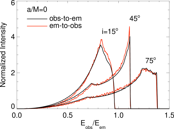
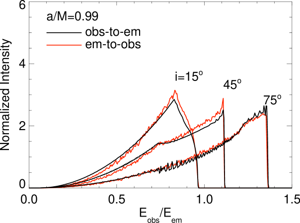
Figure 6: Comparison of observer-to-emitter and emitter-to-observer ray-tracing paradigms for a relativistically broadened emission line. The disk extends from $R_{\rm out}=15M$ all the way to the horizon, and the emissivity profile scales like $r^{-3}$.

In Figure 6, we show the shape of a relativistically broadened emission line as viewed by observers at different inclination angles for the spin values $a/M=0$ and $0.99$. In all cases, the emissivity profile scales like $I\sim r^{-3}$ and the outer disk is truncated at $r=15M$. The disk extends all the way into the horizon, with the fluid velocity inside the ISCO determined by conserving the energy and angular momentum at the ISCO, and solving for $u^{r}$ from the relation $u_{\mu}u^{\mu}=-1$. For the observer-to-emitter calculation, we use the same ray-tracing code described in Schnittman & Bertschinger (2004), with $10^{7}$ photons evenly spaced in the image plane for each inclination. We find excellent agreement in all cases, validating our emitter-to-observer techniques, at least for planar test-particle orbits.

Figure 7: Error estimate $\varepsilon$ as a function of photon number for a relativistically broadened iron line, defined in equation (55). 40 inclination bins were used.

This test in turn naturally leads to a simple convergence test for our Monte Carlo code. Integrating over energy and observer inclination angle $i$, we can apply the following metric to estimate the error due to the use of a finite number of photons:

$$\varepsilon=\frac{\left[\int d\cos i\int dE(I_{\rm lo}(E)-I_{\rm hi}(E))^{2}\right]^{1/2}}{\left[\int d\cos i\int dEI_{\rm hi}^{2}(E)\right]^{1/2}}\,,$$ (55)

with $I_{\rm lo}(E)$ the spectrum calculated at low resolution, compared to the theoretically perfect spectrum $I_{\rm hi}(E)$ calculated at high resolution. As expected for a Monte Carlo calculation, we find that the total error scales with photon number like $N^{-1/2}$, as shown in Figure 7. This is consistent with similar spectral calculations done with the Monte Carlo radiation code grmonty (Dolence et al., 2009). Also shown in Figure 7 are the errors $\varepsilon(N)$ for the observer-to-emitter approach, using a total of 40 inclinations for both cases. We note that the emitter-to-observer method is more than a factor of two more efficient for the same calculation. This is because we can selectively shoot more photons from the inner regions of the disk, but in the reverse method, the photons are distributed evenly in the image plane (this uniform distribution is not strictly necessary; e.g., Noble et al. (2007) use an adaptive grid to improve resolution in bothros).

The next test is similar, but also includes polarization effects. Instead of an emission line with $I(r)\sim r^{-3}$, we use the diluted thermal spectrum for a Novikov-Thorne (NT) disk with an inner edge at the ISCO. The emission has the polarization and limb darkening appropriate for a scattering-dominated atmosphere (Chandrasekhar, 1960). For the observer-to-emitter approach, in addition to utilizing the $I_{\nu}/\nu^{3}$ invariance, we also parallel-transport two polarization basis vectors corresponding to the two axes in the observer plane normal to the photon propagation direction. Then, when the ray intersects with the disk, we calculate a local tetrad in order to determine the local angle of incidence and thus degree of polarization. The direction of polarization is projected onto the parallel-transported basis vectors to give the observed angle at infinity.

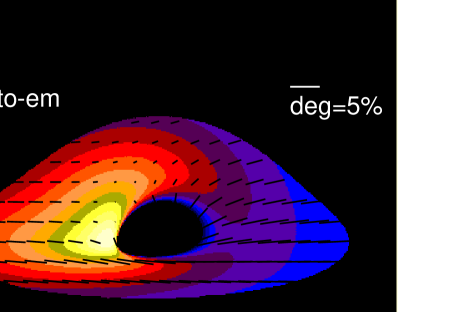
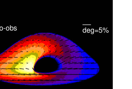
Figure 8: Comparison of observer-to-emitter and emitter-to-observer polarized images for a NT disk with polarization given by a scattering-dominated atmosphere. The disk extends from an inner edge at the ISCO out to $R_{\rm out}=15M$. The black hole has spin $a/M=0.99$ and the observer is at an inclination of $i=75^{\circ}$. The intensity color scale is logarithmic and the polarization vectors are linearly proportional to the local degree of polarization, as observed at infinity.

The two approaches give identical results, as shown in the images in Figure 8, for a Kerr black hole with spin $a/M=0.99$, $R_{\rm out}=15M$, and observer inclination angle 75^∘. The color code is logarithmic in total intensity and covers four orders of magnitude, and the small vectors scale linearly with degree of polarization. For the purposes of comparison, we have not included returning radiation here, despite the important effect it has on the polarization signal (Agol & Krolik, 2000; Schnittman & Krolik, 2009). In fact, it is precisely due to the critical importance of returning radiation that we were forced to employ the emitter-to-observer approach in Schnittman & Krolik (2009, 2010).

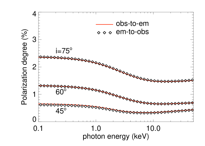
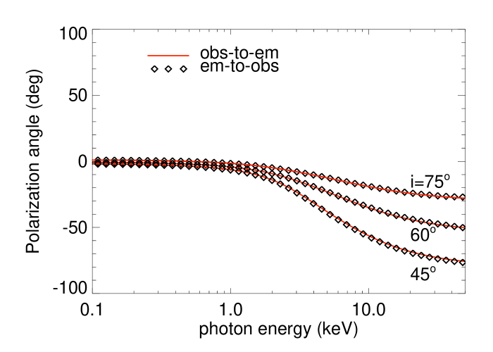
Figure 9: Polarization degree and angle as a function of photon energy for a black hole with spin $a/M=0.99$, luminosity $0.1L_{\rm Edd}$, and mass $10M_{\odot}$. The disk extends from the ISCO out to $r=15M$. The observer-to-emitter (solid curves) and emitter-to-observer (diamonds) methods agree closely over a range of inclinations.

In Figure 9 we show the observables of polarization degree and angle as a function of energy for a range of inclination angles, assuming an Eddington-scaled accretion rate of $\dot{m}=0.1$ and black hole mass $M=10M_{\odot}$. Again, we find excellent agreement between the emitter-to-observer and observer-to-emitter methods.

Figure 10: Outgoing intensity and degree of polarization for radiation emitted from a scattering-dominated atmosphere, as a function of inclination, and for a range of corona optical depths. The face-on orientation is unpolarized due to symmetry.

Next, we move on to testing the coronal scattering algorithms. We focus on a plane-parallel geometry with an optically thick disk covered by a corona with variable optical depth $\tau$ and electron temperature $T_{e}$. In Figure 10 we show the effects of a scattering atmosphere on the emergent flux and polarization as a function of angle. The seed photons are emitted isotropically from the disk surface with zero polarization, then scatter through a cold corona. Photons that scatter back to the disk are reflected via the diffuse scattering formula of equation (53). In the limit of $\tau\to\infty$, we reproduce the limb-darkening and horizontal polarization results from Chandrasekhar (1960), Table XXIV.

Figure 11: Stokes parameters for scattering of unpolarized light off an optically thick atmosphere. See text for description. Compare with Figures 24 and 25 of Chandrasekhar (1960).

In Figure 11 we carry out a similar scattering experiment, but with the seed photons incident from above the disk along a single direction. Setting $\tau=10$, we should reproduce the analytic diffuse reflection expressions of Chandrasekhar (1960), shown there in Figures 24–25 for an incident unpolarized beam with $\cos\theta_{0}=0.8,0.5$ and $\varphi_{0}=0$. Following Chandrasekhar (1960), we plot the Stokes parameters $I$, $Q$, and $U$ as a function of reflection angle, normalized to the incident intensity. The asterisks are the Monte Carlo calculation, and the solid curves are the analytic predictions.

On the left-hand side of each plot, we show the polarization as a function of $\theta$ for $\varphi-\varphi_{0}=0^{\circ},\pm 180^{\circ}$. The value of $\theta_{0}$ is designated with a vertical dashed line. Negative values of $\theta$ correspond to photons reflected back in the general direction of the incident photons, i.e., $\varphi-\varphi_{0}=0$. Thus we see a natural peak in the intensity corresponding to backscattering as in equation (42). Similarly, the degree of polarization is maximized for $90^{\circ}$ scattering, and oriented in the plane of the disk $(Q>0)$.

On the right-hand side of each plot, we show the Stokes parameters for photons scattered with $\varphi-\varphi_{0}=\pm 90^{\circ}$. In this case, the planar symmetry is broken and we find a non-zero value of $U$. Again, the degree of polarization is maximized for scattering angles near $90^{\circ}$.

Lastly, we test the inverse-Compton effects of a hot corona by reproducing the AGN-type spectra of Poutanen & Svensson (1996). The seed photons are again isotropic and unpolarized, with a blackbody spectrum with $T_{\rm bb}=10$ eV. When reflecting off the cold disk, we implement the Compton recoil losses of equation (54). Following Poutanen & Svensson (1996), we also include atomic absorption in the disk with an extremely simple toy model based on the photoelectric cross sections of Morrison & McCammon (1983).

Figure 12: Spectra and polarization of flux from a disk and corona with a slab geometry corresponding to an AGN accretion disk, as described in the text. The solid curves correspond to the total flux, while the (dotted, dashed, dot-dashed, triple-dot-dashed, and long-dashed) curves correspond to $N_{\rm scat}=(0,1,2,3,\geq 5)$. For clarity, only the solid curves are shown for the polarization degree. Compare with Figure 5 of Poutanen & Svensson (1996).

In Figure 12 the corona temperature is 56 keV with optical depth $\tau=0.5$, and in Figure 13 $T_{e}=352$ keV and $\tau=0.05$, corresponding to Figures 5 and 6 in Poutanen & Svensson (1996). In the upper panels we show the observed flux at two inclination angles $\cos i=0.11,0.5$, and in the bottom panels we show the polarization degree $\delta(\%)=Q/I\times 100$. In all panels, the solid curves correspond to the total flux, while the (dotted, dashed, dot-dashed, triple-dot-dashed, and long-dashed) curves represent subsets of the flux, binned by number of coronal scatterings (0, 1, 2, 3, $\geq 5$). Photon packets that return to the disk suffer photoelectric absorption and Compton recoil losses, and are then launched again from the disk, resetting $N_{\rm scat}$ to zero. Thus the dotted curves in Figures 12 and 13 have significant power around the Compton hump at 10-100 keV. As discussed in Schnittman & Krolik (2010), more scatterings in a sandwich corona effectively constrain the geometry and increase the amplitude of polarization at high energies.

We find excellent agreement overall, but are clearly dominated by Monte Carlo noise above $\sim 100$ keV. For these disk and coronal parameters, this corresponds to seed photons that have already scattered on average over 25 times, so it is very difficult to resolve any polarization signal at the few percent level. Additionally, due to our photon packet algorithm, we are limited to energy-independent electron cross sections, so we should expect that the accuracy of our spectral predictions breaks down much above 100 keV anyway.

Figure 13: Same as Figure 12, but for $T_{e}=352$ keV and $\tau=0.05$. Compare with Figure 6 of Poutanen & Svensson (1996).

6 CONCLUSION

We have presented the technical details behind the general relativistic radiation transport code Pandurata. Its capabilities include optically thin emission and absorption, Compton scattering, polarization, spectral and timing analysis, and flexible geometries that allow analysis of numerous accretion models and MHD simulations. We have discussed a number of practical challenges that may also face other teams working to develop similar ray-tracing codes, such as the method of weights in the scattering kernel.

This is by no means the final word on Pandurata. Its great strength lies in its flexibility, and we envisage numerous upgrades and improvements in the near future. These will include, but not be limited to, detailed ionization balance in the disk photosphere for improved AGN modeling, time interpolation between simulation snapshots for generating more accurate light curves, and the inclusion of more sophisticated emission and absorption processes (e.g., angle-dependent synchrotron) to model low-luminosity sources such as Sgr A^∗. Perhaps most important, we will work to close the final remaining gap between theory and observation by incorporating Pandurata  spectra into a data analysis framework like xspec and making it publicly available to the X-ray astronomy community.

Appendix A Hamiltonian Equations of Motion

The equations of motion for the Hamiltonian $H$ in Boyer-Lindquist coordinates, as given in Section 3, are repeated here for completeness:

$$H(r,\theta,\phi,p_{r},p_{\theta},p_{\phi})=-p_{t}=\omega p_{\phi}+\alpha\left(\frac{\Delta}{\rho^{2}}p_{r}^{2}+\frac{1}{\rho^{2}}p_{\theta}^{2}+\frac{1}{\varpi^{2}}p_{\phi}^{2}+m^{2}\right)^{1/2},$$

and according to classical theory:

$$\frac{dx^{i}}{dt} = \frac{\partial H}{\partial p_{i}}\,,$$ (A1a)

$$\frac{dp_{i}}{dt} = -\frac{\partial H}{\partial x^{i}}\,.$$ (A1b)

For convenience of notation, we define the quantity $D^{2}$ as

$$D^{2}(r,\theta,\phi,p_{r},p_{\theta},p_{\phi})=\frac{\Delta}{\rho^{2}}p_{r}^{2}+\frac{1}{\rho^{2}}p_{\theta}^{2}+\frac{1}{\varpi^{2}}p_{\phi}^{2}+m^{2}\,.$$ (A2)

Then for an arbitrary variable $y\in(x^{i},p_{i})$, the partial derivative of $H$ can be written

$$\frac{\partial H}{\partial y}=\frac{\partial}{\partial y}(\omega p_{\phi})+\frac{\partial\alpha}{\partial y}D-\frac{1}{2}\frac{\alpha^{2}}{p_{t}+\omega p_{\phi}}\frac{\partial D^{2}}{\partial y}\,.$$ (A3)

The first set of Hamiltonian’s equations are straightforward to produce:

$$\frac{dr}{dt} = \frac{\partial H_{1}}{\partial p_{r}}=-\frac{p_{r}}{p_{t}+\omega p_{\phi}}\frac{\alpha^{2}\Delta}{\rho^{2}}\,,$$ (A4a)

$$\frac{d\theta}{dt} = \frac{\partial H_{1}}{\partial p_{\theta}}=-\frac{p_{\theta}}{p_{t}+\omega p_{\phi}}\frac{\alpha^{2}}{\rho^{2}}\,,$$ (A4b)

$$\frac{d\phi}{dt} = \frac{\partial H_{1}}{\partial p_{\phi}}=\omega-\frac{p_{\phi}}{p_{t}+\omega p_{\phi}}\frac{\alpha^{2}}{\varpi^{2}}\,.$$ (A4c)

The momentum equations are a bit more involved, but there are only two of them (for $p_{r}$ and $p_{\theta}$; $p_{\phi}$ is conserved):

$$\frac{dp_{r}}{dt}=-\frac{\partial\omega}{\partial r}p_{\phi}+\frac{p_{t}+\omega p_{\phi}}{\alpha}\frac{\partial\alpha}{\partial r}+\frac{\alpha^{2}}{2(p_{t}+\omega p_{\phi})}\left[\frac{\partial}{\partial r}\left(\frac{\Delta}{\rho^{2}}p_{r}^{2}+\frac{1}{\rho^{2}}p_{\theta}^{2}+\frac{1}{\varpi^{2}}p_{\phi}^{2}\right)\right]\,,$$ (A5a)

$$\frac{dp_{\theta}}{dt}=-\frac{\partial\omega}{\partial\theta}p_{\phi}+\frac{p_{t}+\omega p_{\phi}}{\alpha}\frac{\partial\alpha}{\partial\theta}+\frac{\alpha^{2}}{2(p_{t}+\omega p_{\phi})}\left[\frac{\partial}{\partial\theta}\left(\frac{\Delta}{\rho^{2}}p_{r}^{2}+\frac{1}{\rho^{2}}p_{\theta}^{2}+\frac{1}{\varpi^{2}}p_{\phi}^{2}\right)\right]\,.$$ (A5b)

The relevant spatial derivatives are as follows:

$$\frac{\partial\omega}{\partial r} = -\frac{\omega^{2}}{2Ma}\left[3r^{2}+a^{2}(1+\cos^{2}\theta)-\frac{a^{4}}{r^{2}}\cos^{2}\theta\right]\,,$$ (A6a)

$$\frac{\partial\omega}{\partial\theta} = -\frac{\omega^{2}}{2Ma}\left[\left(2Ma^{2}-a^{2}r-\frac{a^{4}}{r}\right)\sin\theta\cos\theta\right]\,,$$ (A6b)

$$\frac{\partial\alpha}{\partial r} = \frac{1}{2\alpha}\frac{\partial\alpha^{2}}{\partial r}\,,$$ (A6c)

$$\frac{\partial\alpha}{\partial\theta} = \frac{1}{2\alpha}\frac{\partial\alpha^{2}}{\partial\theta}\,,$$ (A6d)

$$\frac{\partial\alpha^{2}}{\partial r} = -\alpha^{4}\left(\frac{2M}{\Delta\rho^{2}}\right)\left(\frac{a^{4}-r^{4}}{\Delta}-\frac{2r^{2}a^{2}\sin^{2}\theta}{\rho^{2}}\right)\,,$$ (A6e)

$$\frac{\partial\alpha^{2}}{\partial\theta} = -\alpha^{4}\left[\frac{4Ma^{2}r\sin\theta\cos\theta(a^{2}+r^{2})}{\Delta\rho^{2}}\right]\,,$$ (A6f)

$$\frac{\partial}{\partial r}\left(\frac{1}{\varpi^{2}}\right) = -\frac{2}{\varpi^{4}}\left[\sin^{2}\theta\left(r+\frac{2Ma^{2}\sin^{2}\theta(a^{2}\cos^{2}\theta-r^{2})}{\rho^{4}}\right)\right]\,,$$ (A6g)

$$\frac{\partial}{\partial\theta}\left(\frac{1}{\varpi^{2}}\right) = -\frac{4\sin\theta\cos\theta}{\varpi^{4}}\left[2Ma^{2}\sin^{2}\theta\left(\frac{r^{2}+a^{2}}{\rho^{4}}+\frac{1}{\rho^{2}}\right)+(r^{2}+a^{2})\right]\,,$$ (A6h)

$$\frac{\partial}{\partial r}\left(\frac{\Delta}{\rho^{2}}\right) = \frac{2}{\rho^{2}}\left(r-M-\frac{r\Delta}{\rho^{2}}\right)\,,$$ (A6i)

$$\frac{\partial}{\partial\theta}\left(\frac{\Delta}{\rho^{2}}\right) = \frac{2}{\rho^{4}}a^{2}\Delta\sin\theta\cos\theta\,,$$ (A6j)

$$\frac{\partial}{\partial r}\left(\frac{1}{\rho^{2}}\right) = -\frac{2r}{\rho^{4}}\,,$$ (A6k)

$$\frac{\partial}{\partial\theta}\left(\frac{1}{\rho^{2}}\right) = \frac{2}{\rho^{4}}a^{2}\sin\theta\cos\theta\,.$$ (A6l)

Appendix B Monte Carlo Sampling of Maxwell-Juttner Distribution

For any normalized distribution function $f(x)$ with $x\in(-\infty,\infty)$, one can always define the cumulative distribution function

$${\rm cdf}(x)=F(x)=\int_{-\infty}^{x}f(x^{\prime})dx^{\prime}\,,$$ (B1)

with $F(-\infty)=0$ and $F(\infty)=1$. Then by selecting a uniform random number $\lambda\in[0,1)$, the choice $x=F^{-1}(\lambda)$ will be distributed according to $f(x)$. However, in most cases, $F(x)$ cannot be written in closed form, so other methods are required.

One simple technique described in Press et al. (1992) is the “rejection method,” where an auxiliary function $g(x)$ is used, where $g(x)>f(x)$ everywhere, and $G(x)$ is easy to calculate. We begin by selecting a trial $x_{0}=G^{-1}(\lambda_{0})$, then pick another random deviate $\lambda_{1}$. If $\lambda_{1}<f(x_{0})/g(x_{0})$ then $x_{0}$ is selected as a representative sample of $f(x)$, else we try again with a new $\lambda_{0}$. Of course, if $g(x)$ is large enough, it is easy to ensure that it is greater than $f(x)$ everywhere. However, the efficiency of this method is limited by the ratio of the areas under the two curves $f(x)$ and $g(x)$, so it is desirable to pick $g(x)$ as close to $f(x)$ as possible (Press et al., 1992).

For the Maxwell-Juttner distribution defined in equation (38):

$$f(\gamma)\sim\gamma^{2}\beta\exp(-\gamma/\theta_{T})\,,$$ (B2)

we choose an auxiliary function

$$g(\gamma)\sim\gamma^{2}\exp(-\gamma/\theta_{T})\,.$$ (B3)

This gives

$$G(\gamma)=1-\frac{e^{-\gamma/\theta_{T}}}{e^{-1/\theta_{T}}}\frac{2\theta_{T}^{2}+2\theta_{T}\gamma+\gamma^{2}}{2\theta_{T}^{2}+2\theta_{T}+1}$$ (B4)

for the cumulative distribution function. Inverting (B4) isn’t trivial, but can be done numerically with a simple root finder. For these choices of $f(\gamma)$ and $g(\gamma)$, we find excellent efficiency for this algorithm of $\sim 90$%.

Appendix C Comparison of Scattering Kernels

As described in Section 4, there are (at least) two different ways to implement the scattering of polarized light off of free electrons.

The method of weights picks a random scattering angle from a uniform distribution of $\cos\theta\in[-1,1]$ and $\phi\in[0,2\pi)$, then weights the scattered beam of photons by the cross section in that direction, normalized by the average cross section to conserve flux. By integrating equation (43) over $\phi$, this resembles the classical cross section for unpolarized light:

$$w(\theta)=\frac{I^{\prime}}{I}=\frac{3}{4}(\cos^{2}\theta+1).$$ (C1)

Because repeated scatters tend to increase the level of polarization (indeed, in the microscopic limit, every photon has $\delta=1$), we will focus on the case where $\delta=1$, giving

$$w(\theta,\phi)=\frac{3}{2}(\cos^{2}\theta\cos^{2}\phi+\sin^{2}\phi).$$ (C2)

For angles uniformly distributed in $\cos\theta$ and $\phi$, one can show that the probability distribution function (pdf) for $w$ is

$$P(w)=\frac{1}{3}\left(1-\frac{2}{3}w\right)^{-1/2}$$ (C3)

for $0\leq w\leq 3/2$, and 0 otherwise.

For multiply-scattered photons, the weight function is multiplicative, since the individual scattering events are uncorrelated. For $n$ scatters, the net weight is given by

$$W=\prod_{i=1}^{n}w_{i}.$$ (C4)

To determine the pdf $P(W)$, we define a new variable $Z$:

$$Z\equiv\ln W=\sum_{i=1}^{n}\ln w_{i}=\sum_{i=1}^{n}z_{i}.$$ (C5)

For large values of $n$, the central limit theorem dictates that the distribution of $Z$ should be Gaussian:

$$P(Z)=\frac{1}{\sigma_{z}\sqrt{2\pi n}}\exp\left(-\frac{(Z-n\mu_{z})^{2}}{2n\sigma_{z}^{2}}\right),$$ (C6)

where $\mu_{z}$ and $\sigma_{z}^{2}$ are respectively the mean and variance of $P(z)$. From equation (C3) and the variable transformation $z=\ln w$, we have

$$P(z)=P(w)\frac{dw}{dz}=\frac{e^{z}}{3}\left(1-\frac{2}{3}e^{z}\right)^{-1/2},$$ (C7)

with $z\in(-\infty,\ln 3/2]$. This gives $\mu_{z}=-0.208$ and $\sigma_{z}^{2}=0.710$. Now we see that the pdf $P(W)$ is given by a log-normal distribution:

$$P(W)=\frac{1}{W\sigma_{z}\sqrt{2\pi n}}\exp\left(-\frac{(\ln W-n\mu_{z})^{2}}{2n\sigma_{z}^{2}}\right).$$ (C8)

For photons random-walking through an atmosphere of optical depth $\tau$, we find the pdf of the number of scatters required to escape can be closely approximated by

$$P(n)=\frac{n}{4\tau^{2}}\exp\left(-\frac{n}{2\tau}\right).$$ (C9)

Then the net distribution $P(W)$ for all scatting orders is simply

$$P(W;\tau)=\int_{0}^{\infty}dn\,P(n;\tau)\,P(W;n).$$ (C10)

Figure 14: Relative contribution to the total observed spectrum by photons of a given weight, for optical depths of $\tau=(1,2,3,5,10)$. Any calculation with $\tau\gtrsim 2$ will not formally converge using the method of weights.

The relative contribution to the spectrum from photons with a weight in the range $(W,W+dW)$ is $P(W)WdW$, so we require $P(W)$ to decrease faster than $W^{-2}$ for large $W$ if the calculation is to converge. In Figure 14 we plot $W^{2}P(W)$ for a range of $\tau$. Our analytic results suggest that for $\tau\gtrsim 2$, any polarization spectrum formed using this Monte Carlo weighting method should be dominated by the rarest, highest-weight photon packets, confirming what we have seen in trial runs with large $\tau$. Now, in practice, the convergence is not quite as bad as Figure 14 suggests, for two primary reasons. First, the seed photon packets have little or no polarization, so the initial weighting function more closely resembles equation (C1), which leads to a significantly tighter range in $W$: $\mu_{\rm unpol}=-0.027$ and $\sigma_{\rm unpol}^{2}=0.047$ (in this unpolarized limit, the weight method converges for all optical depths up to $\tau\gtrsim 200$). Second, for the small-to-moderate optical depths of $\tau\lesssim 5$, the typical number of scatters $n$ is still small enough that the mean value theorem does not strictly apply, in effect cutting off the high-weight tails in (C6) and further reducing the contribution from statistical outliers.

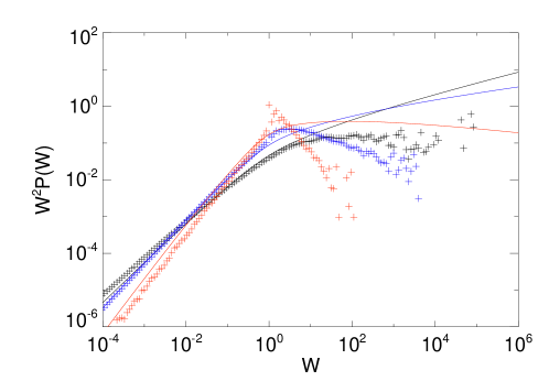
Figure 15: Relative contribution to the total observed spectrum by photons of a given weight, for optical depths of $\tau=(2,5,10)$, sorted by color (red, blue, black). The solid lines are the analytic results, and the crosses are “data” from Monte Carlo calculations of $10^{6}$ photons each.

However, for $\tau\gtrsim 10$, the polarization of a typical photon bundle reaches $\delta\to 1$ after just a few scatters, and the large number of total scattering events allows us to reproduce these analytic results with numerical tests of the Monte Carlo code. In Figure 15 we show the distribution of weights from a calculation using unpolarized seed photons, scattering through optical depths of $\tau=2,5,10$. While we find that the $\tau=5$ case does converge eventually, in practice we find the convergence is so slow that another Monte Carlo method is preferrable. Furthermore, the highest weights have the fewest events, and thus also suffer from small-number statistics, potentially adding to the “undue influence” of outliers. This can be seen in the scatter at the high-weight end of each data set.

Instead of picking a scattering angle at random and weighting it by equation (47), let us use the differential cross section (43) to get the scattering pdf:

$$P(\theta,\phi)=\frac{3}{16\pi}[(1-\delta)(\cos^{2}\theta+1)+2\delta\cos^{2}\theta\cos^{2}\phi+2\delta\sin^{2}\phi]\,.$$ (C11)

Integrating over $\phi$, we again find the standard Thomson cross section (this holds even for $\delta\neq 0$):

$$P(\cos\theta)=\frac{3}{8}(\cos^{2}\theta+1).$$ (C12)

Writing $\mu\equiv\cos\theta$ for convenience, the cumulative distribution function is given by

$${\rm cdf}(\mu)=\int_{-1}^{\mu}P(\mu^{\prime})d\mu^{\prime}=\frac{1}{8}(\mu^{3}+3\mu+4)$$ (C13)

To pick an appropriate value for $\mu$, generate a random number uniformly distributed $\lambda\in[0,1)$, and invert equation (C13), in effect solving for the root of the cubic:

$$\mu^{3}+3\mu+4-8\lambda=0.$$ (C14)

Because ${\rm cdf}(\mu)$ is monotonically increasing, this equation is guaranteed to have a single real root in the interval $-1\leq\mu\leq 1$.

Once $\mu$ is selected, we choose $\phi$ by the same method, now using the pdf

$$P(\phi;\mu)=\frac{1}{2\pi(\mu^{2}+1)}[(1-\delta)(\mu^{2}+1)+2\delta\mu^{2}\cos^{2}\phi+2\delta\sin^{2}\phi]\,,$$ (C15)

which gives

$${\rm cdf}(\phi;\mu)=\frac{\phi}{2\pi}+\frac{\delta}{4\pi}\left(\frac{\mu^{2}-1}{\mu^{2}+1}\right)\sin(2\phi).$$ (C16)

Again, to pick an appropriate $\phi$ given a uniform random $\lambda$, one must invert equation (C16) to get $\phi={\rm cdf}^{-1}(\lambda)$. Unfortunately, this is equivalent to solving Kepler’s equation, which has no closed-form solution, and must be done numerically. Fortunately, this is equivalent to solving Kepler’s equation, one of the best-studied numerical problems in astrophysics! In practice, we use the iterative approach outlined in Murray & Dermott (1999). While slightly more time consuming than the method of weights, the exact cross section method has the distinct advantage of converging for an arbitrary number of scatterings, and thus is the method we prefer for Pandurata.

References

- Agol & Krolik (2000) Agol, E., & Krolik, J. H. 2000, ApJ, 528, 161
- Bardeen et al. (1972) Bardeen, J. M., Press, W. H., & Teukolsky, S. A. 1972, ApJ 178, 347
- Beckwith et al. (2008) Beckwith, K., Hawley, J.F. & Krolik, J.H. 2008, MNRAS 390, 21
- Boyer & Lindquist (1967) Boyer, R. H., & Lindquist, R. W. 1967, J. Math. Phys., 8, 265
- Broderick & Blandford (2003) Broderick, A. E., & Blandford, R. 2003, MNRAS, 342, 1280
- Broderick & Blandford (2004) Broderick, A. E., & Blandford, R. 2004, MNRAS, 349, 994
- Carter (1968) Carter, B. 1968, Phys. Rev. Lett. 26, 331
- Chandrasekhar (1960) Chandrasekhar, S. 1960. Radiative Transfer, Dover, New York
- Connors & Stark (1977) Connors, P. A., & Stark, R. F. 1980, Nature, 269, 128
- Connors et al. (1980) Connors, P. A., Piran, T., & Stark, R. F. 1980, ApJ, 235, 224
- Dexter & Agol (2009) Dexter, J., & Agol, E. 2009, ApJ, 696, 1616
- Dexter et al. (2009) Dexter, J., Agol, E., & Fragile, P.C. 2009, ApJ, 703, L142
- Dexter et al. (2010) Dexter, J., Agol, E., Fragile, P.C., & McKinney, J.C. 2010, ApJ, 717, 1092
- Dexter et al. (2012) Dexter, J., McKinney, J.C., & Agol, E. 2012, MNRAS, 421, 1517
- Dolence et al. (2009) Dolence, J. C., Gammie, C. F., Moscibrodzka, M., & Leung, P. K. 2009, ApJS, 184, 387
- Dovciak et al. (2004) Dovciak, M., Karas, V., & Yaqoob, T. 2004, ApJS, 153, 205
- Dovciak et al. (2008) Dovciak, M., Muleri, F., Goosmann, R. W., Karas, V., & Matt, G. 2008, MNRAS, 391, 32
- Dovciak et al. (2011) Dovciak, M., Muleri, F., Goosmann, R. W., Karas, V., & Matt, G. 2011, ApJ, 731, 75
- Haardt & Maraschi (1993) Haardt, F., & Maraschi, L. 1993, ApJ, 413, 507
- Haardt et al. (1994) Haardt, F., Maraschi, L., & Ghisellini, G. 1994, ApJ, 432, L95
- Huang et al. (2009) Huang, L., Liu, S., Shen, Z.-Q., Yuan, Y.-F., Cai, M. J., Li, H., & Fryer, C. L. 2009, ApJ, 703, 557
- Huang & Shcherbakov (2011) Huang, L., & Shcherbakov, R. V. 2011, MNRAS, 416, 2574
- Johannsen & Psaltis (2010a) Johannsen, T., & Psaltis, D. 2010a, ApJ, 716, 187
- Johannsen & Psaltis (2010b) Johannsen, T., & Psaltis, D. 2010b, ApJ, 718, 446
- Johannsen & Psaltis (2011) Johannsen, T., & Psaltis, D. 2011, ApJ, 726, 11
- Johannsen & Psaltis (2012) Johannsen, T., & Psaltis, D. 2012, ApJ submitted [arXiv:1202.6069]
- Kojima (1991) Kojima, Y. 1991, MNRAS, 250, 629
- Krawczynski (2012) Krawczynski, H. 2012, ApJ, 754, 133
- Laor et al. (1990) Laor, A., Netzer, H., & Piran, T. 1990, MNRAS, 242, 560
- Laor (1991) Laor, A. 1991, ApJ, 376, 90
- Li et al. (2008) Li, L.-X., Narayan, R., & McClintock, J. E. 2008, ApJ submitted, [arXiv:0809.0866]
- Marin et al. (2012) Marin, F., Goosmann, R. W., Dovciak, M., Muleri, F., Porquet, D., Grosso, N., Karas, V., & Matt, G. 2012, MNRAS, 426, L101
- Matt et al. (1993) Matt, G., Fabian, A. C., & Ross, R. R. 1993, MNRAS, 264, 839
- Misner et al. (1973) Misner, C. W., Thorne, K. S., & Wheeler, J. A. 1973, Gravitation (W. H. Freeman, San Francisco)
- Morrison & McCammon (1983) Morrison, R., & McCammon, D. 1983, ApJ, 270, 119
- Murray & Dermott (1999) Murray, C. D., & Dermott, S. F. 1999, Solar System Dynamics, Cambridge University Press, Cambridge
- Noble et al. (2007) Noble, S. C., Leung, P. K., Gammie, C. F., Book, L. G. 2007, CQG, 24, S259
- Noble et al. (2009) Noble, S. C., Krolik, J. H., & Hawley, J. F. 2009, ApJ, 692, 411
- Noble et al. (2010) Noble, S. C., Krolik, J. H., & Hawley, J. F. 2010, ApJ 711, 959
- Noble et al. (2011) Noble, S. C., Krolik, J. H., Schnittman, J. S., & Hawley, J. F. 2011, ApJ, 743, 115
- Novikov & Thorne (1973) Novikov, I. D., & Thorne, K. S. 1973, in Black Holes, ed. C. DeWitt & B. S. DeWitt (New York: Gordon and Breach)
- Poutanen & Svensson (1996) Poutanen, J., & Svensson, R. 1996, ApJ, 470, 249
- Rauch & Blandford (1994) Rauch, K. P., & Blandford, R. D. 1994, ApJ, 421, 46
- Press et al. (1992) Press, W. H., et al. 1992, Numerical Recipes in C: The Art of Scientific Computing (Cambridge: Cambridge University Press)
- Psaltis & Johannsen (2012) Psaltis, D., & Johannsen, T. 2012, ApJ, 745, 1
- Rybicki & Lightman (2004) Rybicki, G. B., & Lightman, A. P. 2004, Radiative Processes in Astrophysics (Weinheim: Wiley-VCH)
- Schnittman & Craxton (1996) Schnittman, J. D., & Craxton, R. S. 1996, Phys. Plasmas, 3, 3786
- Schnittman & Craxton (2000) Schnittman, J. D., & Craxton, R. S. 2000, Phys. Plasmas, 7, 2964
- Schnittman & Bertschinger (2004) Schnittman, J. D., & Bertschinger, E. 2004, ApJ, 606, 1098
- Schnittman & Rezzolla (2006) Schnittman, J. D., & Rezzolla, L. 2006, ApJ, 637, L113
- Schnittman et al. (2006) Schnittman, J. D., Krolik, J. H., & Hawley, J. F. 2006, ApJ, 651, 1031
- Schnittman & Krolik (2009) Schnittman, J. D., & Krolik, J. H. 2009, ApJ 701, 1175
- Schnittman & Krolik (2010) Schnittman, J. D., & Krolik, J. H. 2010, ApJ, 712, 908
- Schnittman et al. (2012) Schnittman, J. D., Krolik, J. H., & Noble, S. C. 2012, ApJ submitted, arXiv:1207.2693
- Shcherbakov & Huang (2011) Shcherbakov, R. V., & Huang, L. 2011, MNRAS, 410, 1052
- Shimura & Takahara (1995) Shimura, T., & Takahara, F. 1995, ApJ, 445, 780
- Sunyaev & Titarchuk (1985) Sunyaev, R. A., & Titarchuk, L. G. 1985, A&A, 143, 374
- Walker & Penrose (1970) Walker, M., & Penrose, R. 1970, Commun. Math. Phys., 18, 265