Is the Sun Lighter than the Earth?
Isotopic CO in the
Photosphere, Viewed through
the Lens of 3D Spectrum Synthesis
Abstract
We consider the formation of solar infrared (2–6 m) rovibrational bands of carbon monoxide (CO) in CO5BOLD 3D convection models, with the aim to refine abundances of the heavy isotopes of carbon (13C) and oxygen (18O, 17O), to compare with direct capture measurements of solar wind light ions by the Genesis Discovery Mission. We find that previous, mainly 1D, analyses were systematically biased toward lower isotopic ratios (e.g., C/13C), suggesting an isotopically “heavy” Sun contrary to accepted fractionation processes thought to have operated in the primitive solar nebula. The new 3D ratios for 13C and 18O are: (); and (), where the uncertainties are 1 and “optimistic.” We also obtained (), but we caution that the observed 12C17O features are extremely weak. The new solar ratios for the oxygen isotopes fall between the terrestrial values and those reported by Genesis (, ), although including both within 2 error flags, and go in the direction favoring recent theories for the oxygen isotope composition of Ca–Al inclusions (CAI) in primitive meteorites. While not a major focus of this work, we derive an oxygen abundance, ppm (relative to hydrogen; on the scale). That the Sun likely is lighter than the Earth, isotopically speaking, removes the necessity to invoke exotic fractionation processes during the early construction of the inner solar system.
1 Introduction
Isotopic ratios of the abundant light elements, especially carbon and oxygen, chart the history of galactic chemical evolution (Langer & Penzias 1993), and closer to home provide insight into fractionation processes that shaped the primitive solar nebula (Krot et al. 2005). Geochemical mixing models that consider only bulk meteorites and terrestrial planets suggest that (inverse) isotopic ratios of the Sun — expressed as, for example, 16O/18O — should be only a few tenths of a percent higher than terrestrial standard values111Based on Vienna Peedee Belemnite [V-PDB] for 13C and the Vienna Standard Mean Ocean Water [V-SMOW] mixture for the oxygen isotopes: Gonfiantini, Stichler, & Rozanski 1995; 12C/13C= (ibid., Table 3), 16O/18O= (ibid., Table 1), and 16O/17O= (ibid., Table 1). (Wiens, Burnett, & Huss 1997), representing an isotopic deficit when expressed per mil222In the solar system context, isotopic abundances conventionally are reported as differences with respect to the standard terrestrial values in parts per thousand () according to, for example, , where is the inverse isotopic ratio commonly quoted in solar work (, for the Sun, is the abundance relative to hydrogen in parts per million [ppm]).. Lunar and Martian isotopic ratios are very close to Earth’s; asteroids traced from meteoritic compositions span a wider range, but still deviate from terrestrial by less than 20 (Burnett et al. 2003); while comets have a mean 13C deficit of (Woods 2009). To be sure, some extraterrestrial materials show even larger isotopic deficiencies, reaching 60 for the oxygen isotopes in Ca–Al inclusions (CAI) of chondritic meteorites in the least altered CAIs (Wiens et al. 2004); while some nebular metal grains show isotopic enrichments in the other direction, up to +180 in the primitive chondrite Acfer 094 (Sakamoto et al. 2007).
One interpretation of the chondritic inclusions led to the prediction that the Sun should be similar to the isotopically lightest CAIs (Clayton 2002). Compositions of solar wind ions implanted in lunar metal grains covered the range from 16O enriched (rare isotopes depleted) and similar to the lightest CAIs (Hahsizume & Chaussidon 2005), to 16O depleted (rare isotopes enhanced), more like atmospheric ozone (Ireland et al. 2006). NASA’s Genesis Discovery Mission resolved the conundrum by measuring solar wind isotopes to extremely high accuracy through direct capture of the light ions (Burnett et al. 2003). Analysis of Genesis collection plates found and , which implied photospheric values of for both isotopes, after accounting for fractionation due to inefficient Coulomb drag during solar wind particle acceleration (McKeegan et al. 2011).
The Genesis photospheric values are consistent with the isotopically lightest CAIs, in line with Clayton’s prediction, and imply that a mass-independent fractionation (MIF) process occurred between the Sun and terrestrial planets during solar system formation. Proposed mechanisms for the MIF include CO self-shielding in the solar nebula (Clayton 2002; Lyons & Young 2005); CO self-shielding in the molecular birth cloud (Yurimoto & Kuramoto 2004; Lee, Bergin, & Lyons 2008); galactic chemical evolution of interstellar gas and dust with differing time scales, in this case with the dust younger than the gas (Krot, Nagashima, & Ciesla 2010); and a chemical MIF accompanying O3 formation in surface reactions on dust grains, which then is imparted to molecular cloud water (Dominguez 2010). Large oxygen isotope effects in CO self-shielding have been measured in at least one molecular cloud (Sheffer, Lambert, & Federman 2002), and in a proto-planetary disk as well (Smith et al. 2009), but with large enough error bars to preclude confirmation of a slope similar to the CAI mixing line.
Spectroscopic determinations of photospheric isotopic abundances offer a different, somewhat contrary, perspective. An early study by Hall, Noyes, & Ayres (1972) of the 2.3 m overtone rovibrational bands of solar carbon monoxide at the McMath-Pierce telescope on Kitt Peak derived a 12C/13C ratio of 90 with an uncertainty of 15% (at 95% confidence level), consistent with the terrestrial value of 89. The measurements were made in a sunspot, where thanks to the cooler temperatures, the isotopomer transitions attained far greater strength than in the warm photosphere. Overtone transitions of 12C18O and 12C17O were not discernible in the 2.3 m umbral spectrum, however. A follow-up study by Hall (1973) extended the isotopic measurements to the 4.6 m fundamental bands, in the undisturbed photosphere as well as sunspots, using a newly commissioned infrared grating spectrograph at the McMath-Pierce. He derived a slightly lower 12C/13C ratio of 848, but still consistent with terrestrial. Hall also estimated values for 18O and 17O, again obtaining essentially terrestrial ratios, although with large error bars.
While the CO isotopomer bands are strongly enhanced in sunspots, so too are those of other molecules, leading to complex spectra with substantial line crowding. For this reason, photospheric observations are preferred for the isotope problem, because the warmer temperatures favor durable CO over its more weakly bound cousins like OH and SiO, leading to cleaner, less crowded spectra. Even so, from the ground there are only a few usable windows in the infrared for the CO measurements, owing to heavy molecular blanketing by the Earth’s atmosphere.
Addressing both these issues, Harris, Lambert, & Goldman (1987) recorded the photospheric CO fundamental bands with a Fourier transform spectrometer (FTS) during a high altitude balloon flight. Adopting the Holweger–Müller (1974) 1D reference temperature stratification (very similar to contemporary 1D semi-empirical models), they derived 12C/13C= and 16O/18O= . The 12C17O spectrum was too weak in their scans to measure. Again, the observed solar ratios were slightly lower than terrestrial, but within the cited uncertainties.
More recently, Ayres, Plymate, & Keller (2006; hereafter APK) analyzed an extensive, high quality record of the solar CO fundamental and first-overtone bands from the Shuttle-borne ATMOS FTS, supplemented with ground-based disk center and limb scans obtained with the large 1 m FTS at the McMath-Pierce. The authors synthesized CO line profiles, and center-to-limb behavior, utilizing a variety of 1D photospheric reference models, and multicomponent variants intended to simulate at least the thermal impact of the convective fluctuations that characterize the inhomogeneous solar plasma. Their recommended values of the isotopic ratios were: 12C/13C= , 16O/17O= , and 16O/18O= , where the cited small uncertainties represented standard errors of the mean (1 s.e.) over the large samples of parent (12C16O) and isotopic CO transitions considered, but exclusive of possible systematic errors. These ratios, taken at face value, were significantly lower than terrestrial. At the same time, a pioneering study by Scott et al. (2006; hereafter SAGS) of solar CO and the associated isotopomers, again based on the ATMOS material but now using prototype 3D convection models, proposed isotopic ratios 12C/13C= and 16O/18O= ; higher than APK, slightly lower than terrestrial, but agreeing with both within (2 ) uncertainties.
Notably, while the recent studies found solar 12C/13C ratios generally consistent with terrestrial, when aggregated together, they all were systematically lower, rather than, say, scattering uniformly around the standard value. Unfortunately, the uncertainties still were too large to distinguish between an isotopically “heavy” versus “light” Sun, especially for 18O and 17O, which as described earlier display a 6% deficit relative to ocean water according to Genesis. A more precise measurement of photospheric 12C/13C, as well, might help to distinguish between the several proposed MIF mechanisms. For example, CO self-shielding should initially impart a large depletion of 13C16O in the solar nebula, yet that would be removed at least partially, and possible entirely, by subsequent ion-molecule charge exchange reactions between C+ and CO. The potentially broad range of depletions has yet to be meaningfully constrained by model calculations, so an accurate measurement of the photospheric ratio could provide some needed guidance.
Here we reconsider the solar CO isotopic analysis, in light of a more recent generation of solar 3D models, which now meet key observational tests that the initial complement of convection simulations was less successful matching. We also have taken special precautions, on the one hand to control and narrow the random (mainly observational) uncertainties of the analysis; and on the other to quantify a variety of systematic effects related to the models, and equally so the laboratory molecular line parameters. We stress that we are attempting to perform precision “forensic” spectroscopy of the solar plasma with uncertainties ideally below 1%, in order to compare to the very precise Genesis findings (with 1% quoted errors). To preview our conclusions, that goal was frustrated by lingering uncertainties in the atomic physics (-value scales) and more subtle aspects of the modelization, even though state-of-the-art 3D convective snapshots were utilized. Nevertheless, we also demonstrate that especially for 13C, but 18O as well, the observational uncertainties can be controlled to the desired level or better, so that in principle future comparisons of higher precision can be carried out, once the external atomic physics and modelization issues are resolved. We also confirm that the 1D spectrum synthesis approach is essentially useless for this particular molecular problem, although to be sure there are other less pathological cases where a careful 1D analysis can produce similar results to a full 3D study (see, e.g., Ayres 2008).
2 Observations
There is a clear advantage of infrared molecular spectra for tracing photospheric isotopic abundances, as noted in Hall, Noyes, & Ayres (1972): the isotopomer and parent (12C16O) rovibrational transitions are well separated in frequency, (in wavenumbers [cm-1]), owing to the large influence of the different molecular weights on the rotational and vibrational properties of the respective diatoms. Isotopic shifts encountered in the electronic spectra of atoms and ions are minuscule in comparison, and usually much smaller than the thermal line width at photospheric temperatures, rendering isolation of the isotopic component rather tricky, if possible at all.
At the same time, obstacles encountered in an isotopic analysis of solar molecular features are myriad. First, the heavy isotopes of C and O have very low abundances and consequently their absorption lines tend to be weak. These will be more influenced by unrecognized blends, especially in telluric contaminated ground-based spectra, than their much stronger 12C16O counterparts. Second, the strongest isotopomers are fundamental transitions at the peak of the rotational distributions (), but the equivalent parent 12C16O lines are too strong to be useful in an abundance study (Hall 1973). Consequently, the isotopic lines must be compared to intrinsically weak parent lines — high excitation transitions in the case of — thereby creating the possibility of biases in the highly temperature sensitive analysis. Finally, historically there have been significant disagreements among proposed oscillator strengths for the “hot” CO bands (see, e.g., APK).
To be sure, many of these challenges have straightforward solutions. For example, the dominant cause of blending in the CO bands are other CO lines, whose frequencies are precisely known and whose relative strengths can be estimated by spectrum synthesis. Thus, minimally contaminated features can be readily identified. Further, in an isotopic analysis, the absolute accuracy of the oscillator strength scale is not as important as the relative precision (e.g., , where the subscript is the isotopomer designation: C16O, and so forth) over the rotational ladder, given that the relative scalings for the isotopomer -values depend on ostensibly simple atomic physics considerations, and should be calculated consistently even when the absolute parent strengths might be in error. Additionally, one can consider features covering a range of lower level excitation energies, , to help identify temperature-dependent trends, which might arise from systematic deviations of the oscillator strengths with , which is correlated with , or from the solar model itself. Even so, the analysis probably would not be possible if it were not for the existence of very high-quality FTS scans of the average disk center solar spectrum, free of telluric contamination and in the relevant portions of the infrared, from the space-based ATMOS FTS experiment.
2.1 ATMOS
As noted in APK, Shuttle-borne ATMOS was a high-resolution () FTS instrument designed to study trace molecular species in the Earth’s atmosphere backlighted by the rising or setting Sun as viewed from low-Earth orbit. Solar reference spectra, obtained from zenith pointings, were free of terrestrial contamination. The instrument recorded a diameter circular region at disk center, which corresponds to for all intents and purposes (, where is the heliocentric angle). The best results were obtained from the final ATMOS flight in 1994 November as part of the ATLAS-3 payload (Abrams et al. 1999). The signal-to-noise of those data is extremely high, better than ; well suited for a study like the present one, which must dig down to the very weak isotopic features. Based on clean ATMOS CO lines in common to even higher-resolution McMath-Pierce FTS measurements, we adopted a 2 km s-1 FWHM Gaussian approximation to the ATMOS instrumental profile to smooth synthetic CO spectra for comparison with observed line shapes. Details concerning the reduction of the dearchived ATMOS scans can be found in the earlier paper (APK).
2.2 Hybridization of ATMOS Spectral Features:
12C16O and , and the
Isotopomers
As alluded earlier, the solar CO bands contain large numbers (literally thousands) of absorption lines, many of which, especially 12C16O, are minimally contaminated by extraneous features. Further, because of the modest, smooth change of -value and excitation energy along the rotational ladders of each vibrational band, lines of similar rotational numbers in the same band are very similar to one another in absorption strength: spectral clones if you will. Having a large sample of target transitions potentially is a great benefit, especially to help isolate systematics. In contrast, abundance studies based on only a few accessible features — like photospheric atomic oxygen — become more susceptible to accidental blends, distortions in the local continuum level, and NLTE excitation (e.g., Caffau et al. 2008). Synthesizing absorption profiles of hundreds of CO lines is a trivial matter in classical 1D spectral analysis, but is less attractive for 3D work, where each temporal snapshot is equivalent to tens of thousands of 1D problems, and a dozen or more snapshots well separated in time should be considered to ensure an adequate average.
We worked around the tension of wanting to consider as many CO features as possible, but at the same time minimizing the number of transitions to synthesize in 3D, by combining groups of CO lines of similar excitation, wavenumber range, and absorption depth together to yield “hybrid” features. In this way, we could distill the properties, both observational and laboratory, of perhaps a 150 separate absorptions into a smaller, more tractable sample of a few dozen or so, with increased S/N and better defined continuum levels. For this study, we restricted lower level energies to below 18,000 cm-1, which characterizes the majority of the measurable isotopomer features. The goal then was to develop a comparison sample of fundamental and overtone parent lines in this energy interval, as well as the isotopic sample itself. Initial line shape synthesis tests suggested that beyond an equivalent width, , of about 5 mKy (10-3 cm-1), a typical CO line begins to saturate, and thus becomes less responsive for an abundance analysis. The saturation limit for lines is about twice as high. We thus also applied these respective cutoffs as part of our line selection criteria.
In practice, the and cuts severely limited the number of suitable features that could be “hybridized;” many more lines were available, however. This is an important issue because all of the best (i.e., highest S/N) isotopomer features are of the type. Ideally, parent lines and the isotopomer counterparts should be compared on as close to the same basis as possible, to avoid potential systematic errors that might creep into the analysis by, say, pitting isotopomers against parent lines (the overtone oscillator strengths are smaller by a factor of 100). Because of the relative scarcity of suitable target lines — parents typically too strong, isotopomers typically too weak — we were forced to collect them without paying too much attention to the combinations, but rather more closely to (the fundamental quantity that controls the number of absorbers through the Boltzmann factor).
We identified suitable lines for hybridization by considering visualizations of all the CO features that satisfied the and cutoffs, and did not have another 12C16O transition with any significant strength whose line center fell within km-1 of the target line (i.e., not close enough to disrupt the candidate line, given the typical 4.4 km s-1 line full width at half maximum intensity [FWHM]). The visualizations compared the observed line shape to simulations from the FAL-C 1D model (Fontenla, Avrett, & Loeser 1993), with abundances adjusted (as a function of , as described later) to achieve reasonable matches to known clean 12C16O lines, and separated according to isotopomer. In this way, blends of 12C16O target lines with, say, weak coincidental isotopic features could be identified. In order to increase the number of potential hybridization candidates, lines were included that were affected in their far wings (beyond km s-1) by blends, as long as the nearest edge of the blend terminated short of the target absorption, and as long as the local continuum level appeared to be adequately defined in at least one of the wings. The affected parts of the target profile were ignored when the candidates subsequently were coadded. A list of potentially suitable features was compiled in this way.
That list then was parsed into groups of transitions nearby in wavenumber, close in , and similar in absorption depth. The hybridization candidates in each group were aligned by Gaussian centroiding, interpolated onto a finely sampled velocity scale (0.5 km s-1 steps), and coadded, evenly weighted, ignoring the portion(s) of the line profile previously flagged as corrupted (trimming was limited to velocities outside the km s-1span of the line core).
At the same time, the parallel collection of individual molecular parameters also was “hybridized.” The approach was to average the line strengths (-values) and the temperature- and wavenumber-dependent components of the absorption — stimulated emission and Boltzmann excitation factors — for a set of discrete temperatures between 4000 K and 5000 K, then fit the resulting average relation with an optimal combination of -value and (after setting the transition frequency to a weighted mean of the group). Note that the for the R- and P-branch transitions of the same are the same, as is the statistical weight , but in general the oscillator strengths will differ, favoring the R-branch, and the difference increases up the rotational ladder (as illustrated later, in Fig. 1a). The molecular parameters were hybridized for two independent oscillator strength scales, as decribed next, and for a third scale — — which was a straight average of the two.
2.2.1 Oscillator Strengths
We considered two independent oscillator strength scales for the study: Goorvitch (1994: G94), based on experimentally derived transition matrix elements; and Hure & Roueff (1996: HR96), who utilized theoretical electric dipole moment functions. Figure 1a illustrates the dependence of and oscillator strengths separated by vibrational band, as a function of lower rotational level, , as derived from the HR96 dipole matrix elements, and for a version of the G94 –values taken from the HITEMP section of the HITRAN database333see http://www.cfa.harvard.edu/hitran/.
We chose the HITRAN CO line strengths, which were derived from the G94 matrix elements, because the HITRAN values are given to higher precision than the original G94 electronic tabulations. However, a detailed comparison of HITRAN to the G94 scale showed that the latter was systematically very slightly higher (by 0.25%), independent of , for both fundamental and first overtone; except for the 2–0 band444The vibrational band designation is –, where the leading value is the upper vibrational level, the trailing is the lower, and 1, 2 for the fundamental and first overtone, respectively. Note, also, that the rotational lines in a given fundamental or overtone band can be in one of two branches: “P” if the upper state is one lower than the initial state (); and “R” if the upper state is one higher (). which showed a much larger shift (%), with a strong increase for higher in the P branch, but not the R branch. The small systematic offset undoubtedly can be traced to a slightly different numerical value for the combined physical constants that appear in the conversions from matrix elements to Einstein –values and ultimately -values; but the larger -dependent offset for the 2–0 band likely signals a more significant numerical issue. Ratios of oscillator strengths between neighboring bands (e.g., ) at the same show very systematic behavior. On this basis, the HITRAN 2–0 band appears to be anomalous. We thus corrected the HITRAN 2–0 band to the G94 scale, and adjusted the rest of the HITRAN and values for the slight deficit mentioned earlier.
Figure 1b compares ratios of the G94 to HR96 oscillator strengths on an expanded scale to illustrate the differences more clearly. The G94 -values are systematically a few percent lower than those of HR96, but independent of vibrational band or rotational number. In contrast, the overtone bands tend to have larger oscillator strengths on the G94 scale, at least for the lower vibrational bands, and the deviations relative to HR96 vary strongly and systematically with both vibrational band and rotational number.
Figure 1c compares -values of 13C16O to 12C16O on the G94 and HR96 scales separately. The isotopomer strengths are smaller by about 4%, essentially identical on the two scales, and show minimal dependence on or . A similar deficit is seen for the oxygen isotopes: 12C17O is down by 2% and 12C18O by 4%. The consistent behavior between the two oscillator strength scales supports the premise stated earlier that the relative precision of the isotopomer -values should be better determined than the absolute parent values.
2.2.2 Equivalent Widths
After the hybrid profiles were constructed, equivalent widths were measured. First, a continuum level was established by considering the intensities on either side of, but well away from, line center (in practice, 6 km s-1 km s-1). An “Olympic” filter (throwing out the two highest and two lowest values) was applied to the collection of (nine) points in each flanking continuum band separately, and the larger of the medians of the two sets of surviving points was adopted as the continuum level. The dispersion of the normalized points in the flanking reference continuum windows served as an empirical estimate of the photometric noise, which later was utilized to assign an uncertainty to the equivalent width according to the FTS noise model of Lenz & Ayres (1992).
The equivalent width, itself, was measured by fitting a Gaussian profile to the normalized intensities within km s-1 of line center (which now was located very close to zero velocity owing to the initial centroiding of the constituent profiles). Although the solar CO lines display a systematic convective blueshift of around 350 m s-1, the profiles nevertheless are very close to Gaussian in shape (with a FWHM of around 4400 m s-1 for the weak fundamental and overtone lines, but C-bisector amplitudes of only a few hundred m s-1 [SAGS]). The Gaussian fitting approach was adopted here (and in the previous work of APK) because as applied (later) to the synthesized profiles, it allows the use of a sparsely sampled frequency grid. This is advantageous in the computationally challenged 3D setting.
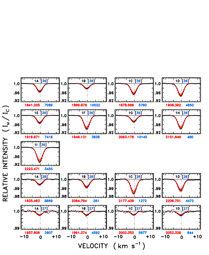
The initial sample of hybrid features was subjected to an abundance analysis in a representative 3D snapshot using the average oscillator strengths, to derive an consistent with the observed equivalent width for each line separately (see below for details). The resulting distributions of inferred with both and were examined, and any deviants from the expected smooth relations were culled out. The offending hybrids were vetted to see whether one of the constituent lines was anomalous with respect to the others (affected perhaps by an unrecognized non-CO blend), and if eliminating the offending line could improve the behavior. If not, the outlier hybrid was simply discarded. Ultimately, through this iterative, somewhat arbitrary, process a final sample of 36 hybrid parent lines was developed, 10 and 26 , from about 150 input transitions. Table 1 summarizes the constituent lines and final hybrid parameters (for the scale). Figure 2a illustrates the procedure for four representative hybrids, and Figure 2b similarly for four cases. Note in Table 1 that the hybrid designated 1J26 is the trivial case of a single line, because only one suitable could be found for the (key) energy range below 7000 cm-1. Also, we caution that the Gaussian parameters (, FWHM) listed for the individual contributing lines in a hybrid group should be taken only as a guide, especially for those features with distortions in one wing or the other: the continuum level in the pre-coadded profiles is less well defined than for the final hybrid owing to higher photometric noise and the possible influence of intensity deviations, due to blends, outside the line core. This caution particularly extends to the isotopic sample described next.
The hybridization scheme was applied in a similar fashion to 13C16O, 12C18O, and 12C17O (9, 4, and 4 hybrids, respectively, representing nearly 70 input transitions). For the isotopomers, the Gaussian fitting imposed a fixed FWHM of 4.14 km s-1, as inferred from the average of the measured widths of the higher-S/N 13C16O hybrids. The apparent decrease with respect to the FWHM km s-1 of the narrowest parent profiles is somewhat more than expected from the influence of the larger molecular weights on the thermal broadening, but the decrease is replicated in the 3D line shapes of the isotopomers. In addition, the Gaussian centroiding step, prior to coadding, was omitted in favor of accepting the laboratory line centers on the ATMOS frequency scale. (An empirical zero-point calibration of the ATMOS velocity scale was determined for each isotopomer separately according to the mean shift of the hybrid lines relative to 1D synthesized profiles, determined in an initial fitting step.) Examples of the isotopomer hybrids are illustrated in Figures 2c (13C16O), 2d (12C18O) and 2e (12C17O). The calculated hybrid line parameters are summarized in Table 2, again for the reference scale.
3 Analysis
In overview, our strategy was first to derive an oxygen abundance for a given solar model using the 12C16O “parent” hybrid line sample, then calculate the isotopic ratios that reproduced the equivalent widths of the weak isotopomer absorptions for that oxygen abundance. This was done in practice by synthesizing the hybrid line equivalent widths for a small set (4–6) of discrete values [of the oxygen abundance, ; or scale factors, , relative to reference isotopic ratios, , where , e.g., refers to 12C/13C] spanning the full range of potential sample variation, and then interpolating with the observed to deduce the corresponding target value (of or ). For convenience, we assumed , so that the CO concentration effectively becomes quadratically dependent on the oxygen abundance (see APK for the physical motivation behind this choice).
The derived ’s in the first step typically were found to depend systematically on (see SAGS; APK), and usually there was an offset between the and hybrids as well. The abundance gradients and fundamental/overtone shifts could be due to: (1) systematic errors in the -value relations as a function of (which correlates with ); or (2) small thermal differences between the 3D convection models and the real Sun in the CO-absorbing layers (the middle photosphere, well above the continuum-forming zone: see APK and Fig. 3b, below). That the ab initio 3D models might depart somewhat from the true Sun in the mid-altitudes of the photosphere would not be Earth-shattering, because the underlying simulations typically are purely radiation-hydrodynamic, lacking the small-scale magnetic fields of the true photosphere (Stein 2012), and usually also missing high-frequency acoustic waves (with wavelengths not resolved by the grid spacing in the computational box), which are strongly damped in the outer photosphere (Ulmschneider 1974). Both of these neglected phenomena potentially could produce additional heating there (e.g., Ayres 1975).
We thus also considered slightly perturbed models for which the thermal structure above the continuum-forming layers was systematically raised by a small amount ( K) so that the resulting mean temperature stratification matched that of a semi-empirical 1D reference model. In these temperature-enhanced models, we usually found a significantly different slope of against , and that the and samples displayed an opposite offset compared with the baseline. We then imposed an intermediate temperature correction chosen specifically to force the and samples to agree. In principle, this middling “Goldilocks” solution represents an atmospheric model whose thermal structure is in harmony with respect to the CO fundamental and overtone bands; but, as we show later, the specific temperature correction does depend on the adopted oscillator strength scale.
We pursued this tripartite strategy for the G94 and HR96 CO oscillator strengths separately, to test for potential systematic errors from that source. When calculating the isotopomer hybrid samples, we imposed the specific relation inferred for the parent hybrids (since all the isotopic lines are of the type). We strove to attain as much consistency at each level of the analysis as possible, but also to explore as much of the potential parameter space as was permitted (by other constraints) to judge by how much the final results might be influenced by the models and/or molecular parameters. The individual pieces of the strategy are described in more detail next.
3.1 CO5BOLD 3D Snapshots and Continuum Tests
We adopted the so-called “CO5BOLD” radiation-hydrodynamic (RHD) scheme to provide the baseline 3D models for the CO infrared spectral synthesis. The methodology behind the CO5BOLD 3D stellar convection simulation code has been described by Freytag et al. (2012), who have compared results from this and other contemporary 3D RHD simulations, with excellent agreement achieved for key tests such as visible continuum center-to-limb behavior (see, also, Beeck et al. 2012). Wedemeyer-Böhm & Rouppe van der Voort (2009) have examined photospheric intensity distribution functions in blue, green, and red continuum bands, at disk center and near the limb, from Hinode Solar Optical Telescope images (corrected for point response and stray light), and concluded that the CO5BOLD 3D simulations well reproduced the various observables that characterize the granular fluctuation patterns. This agreement gives us confidence for the infrared problem, since the 2.3 m and 4.6 m continua bracket the formation depths of the visible radiation.
We utilized sixteen independent 3D snapshots, well separated in time, from a fully-relaxed CO5BOLD run. This is a slightly reduced set of those employed by Caffau et al. (2008) in their analysis of photospheric atomic oxygen: see that study for more modelization details. Figure 3a illustrates schematic temperature and velocity maps for the snapshots collectively, for a constant height slice (median of the dyne cm-2 pressure surface) characteristic of the deep photosphere where the visible continuum arises. There are a dozen, or so, identifiable granules in each snapshot, which have the familiar broad, warm upwelling centers, surrounded by narrower, cool subducting lanes. The area asymmetry largely is responsible for the convective blueshifts seen in most photospheric lines.
Each snapshot has 40 km steps in the two horizontal directions, covering a 5.65.6 Mm2 patch of the surface, and 15 km grid steps in the vertical direction, with an extent of 2.3 Mm; altogether a resolution of 140140150. The top boundary of the snapshots was very high ( in Rosseland optical depth), well above the CO-absorbing layers in the middle photosphere; and for convenience we truncated the vertical grid at a maximum depth such that at any relevant frequency, thus ignoring the deepest layers that are important for the deep-seated granulation dynamics, but not the CO spectrum synthesis confined to the surface layers.
Twelve opacity bins were utilized for the radiation transport in the RHD simulations, a significant improvement over earlier generations of such models that were derived using only one or a few radiative bands. Abundances were taken from Grevesse & Sauval (1998), except for CNO where values closer to Asplund, Grevesse, & Sauval (2005) were adopted. The fact that the 3D time series was calculated with CNO abundances that we later show are inconsistent with what we find from CO is not vital, because: (1) the CNO abundances are not critical to the model pressure structure (the metals that provide the electrons for the H- opacity are far more important); and (2), we apply a “calibration” adjustment to the model pressure scales to compensate for any slight such inconsistencies, as outlined next.
As described in a previous 3D study (of [O I] 6300; Ayres 2008), an important practical consideration in utilizing “imported” RHD models is that there might be slight inconsistencies between the opacities and equation of state employed in the original simulation, and the (usually more detailed) ones embedded in a post facto spectrum synthesis code. Such inconsistencies could lead, for example, to the prediction of slightly different continuum intensities (say, in the visible) than were inherent in whatever effective temperature constraint was imposed at the lower boundary of the 3D simulation. We mitigated against such inconsistencies by requiring that the full 3D model (consisting of the 16 independent snapshots) successfully predict absolute continuum intensities (see, e.g., APK) over the visible range 0.44–0.68 m. We forced such agreement by slightly adjusting the pressures in the model by a uniform multiplicative factor. The slight shift of the pressure scale moves the steep part of the deep-photosphere temperature profile, where the visible continuum forms, inward or outward in optical depth space, thereby changing the temperatures where the continuum becomes optically thick, and thus the emergent intensity field. For this particular multi-snapshot CO5BOLD model, the derived scale factor was 1.033: a small correction, to be sure, given the potentially large inconsistencies that in principle could be found in such a comparison. The pressure adjustment has much less impact on the middle photosphere, where the temperatures have flattened out compared to the deeper layers.
Also highlighted in Fig. 3a are three snapshots selected for a more detailed analysis to examine the role of systematic effects, for example arising from the stochastic nature of the independent thermal profiles (i.e., how many snapshots are needed for a reliable average) or from the oscillator strength scales (which have a subtle impact on the “Goldilocks” balance temperatures mentioned earlier). Snapshot “B” has an average upper photospheric temperature profile very similar to that of the full model; snapshot “A” is cooler than average at high altitudes; and snapshot “C” is warmer than average. In general, these temperature deviations are reversed at depth. Also, the pressure scale factor derived from the full 3D model was applied to the individual reference snapshots, rather than deriving a specific scale factor for each, in order to preserve the stochastic intensity fluctuations inherent in such snapshots (although it turned out, by accident, that the three reference snapshots have nearly identical visible continuum intensities, all slightly above the full 3D model).
Figure 3b compares a spatially averaged (on surfaces of constant pressure) version of the full 3D model to the FAL-C semi-empirical 1D stratification. Also shown is the result of applying a uniform temperature shift of +90 K to the outer layers of the 3D model, so that the pressure-surface average more closely resembles the temperature profile of the semi-empirical model. (We subsequently refer to such a temperature-enhanced 3D model as the “maximally perturbed” scenario, or MAX for short.) The figure includes depth distributions of CO densities, calculated in the models for the same (600 ppm), and again averaged on constant pressure surfaces; together with formation depths of the visible continuum (0.5 m), and those at the CO overtone (2.3 m) and fundamental (4.6 m). Although the 1D FAL-C and the MAX variant of the 3D model share the same average stratification in the CO layers, MAX evidently produces significantly more CO, presumably because the gain in molecular formation in the downward temperature fluctuations more than compensates for the loss in the upward ones. This 1D–3D difference is exaggerated for the CO problem owing to the large, non-linear temperature sensitivity of the molecular chemistry.
Figure 4 illustrates predicted absolute disk center continuum intensities and center-to-limb behavior at , quite close to the limb, for the three representative snapshots. The underlying observations were described previously in APK, and the 3D continuum synthesis approach in Ayres (2008). In short, Planck functions (thermal emission term) and continuum opacities for each vertical column of the 3D model were interpolated from precalculated tables, according to the local temperature and pressure. Next, the continuum source functions (including Thomson and Rayleigh scattering) were calculated. For simplicity, we implemented a “1.5D”5551.5D means treating each column of the 3D model as an isolated, laterally homogeneous atmosphere to solve for the angle-dependent radiation fields in the local scattering term. This approximation is valid for the visible continuum, for which the scattering component is small, and the scattering mean-free-paths are short compared to the horizontal variations of the convective structures. In the IR, the approximation is irrelevant, because the scattering term is insignificant, and the source function equals the local Planck function. partial coherent scattering (PCS) formalism, on the native optical depth scale of each vertical column, using the Feautrier-based Hermitian method of Auer (1976). Given the continuum source functions, , for each column, 3D specific intensities then were calculated along rays (vertical for disk center, inclined for the limb) according to the formal solution of the transport equation. This was accomplished in practice by interpolating the vertical source functions and opacities onto the rays (which intersect multiple columns for the limb viewing case), and then interpolating the newly derived ray source function onto a fixed optical depth grid, with associated precalculated Feautrier coefficients, to achieve a fast but accurate formal solution for the emergent intensity.
To achieve higher accuracy for the vertical transport calculations, the columns were interpolated onto a finer, 5 km grid. For the limb sightlines, the models were resampled onto a finer, 20 km horizontal grid, and the views from the four cardinal azimuthal directions (, ) were averaged (in practice, the differences between the independent views were minimal).
Referring back to Figure 4, there are two sets of center-limb curves depicted. Generally, the lower ones are for the baseline 3D snapshots, while the slightly higher ones are for the temperature-enhanced MAX versions. It is clear that not only do the baseline snapshots reproduce the continuum center-limb behavior reasonably well (and much better than the initial generation of 3D models, which solved the radiation transport utilizing only a few opacity bins), but also the high-altitude temperature perturbation has essentially no influence on the disk center continuum intensities and minimal impact on the center-limb behavior. This is a consequence of restricting the temperature rise to the higher, transparent layers.
We consider the MAX option to be an extreme case, because the contrived match of the mean 3D model to the 1D profile glosses over important aspects of how spatial averages of different spectral diagnostics feed into the practical construction of a semi-empirical model. Nevertheless, it is encouraging that the simple high-altitude temperature enhancement does not fundamentally violate the “continuum test.” We included the temperature-enhanced snapshots in the CO modeling as a hedge against the possibility that the purely RHD 3D simulations might be slightly too cool in their outer layers, owing to lack of magnetic heating effects and/or damping of high-frequency acoustic waves, as noted earlier. The derived MAX temperature enhancements for the three reference snapshots, treated as independent models, ranged from 75 K (“C”) to 110 K (“A”), with “B” — and the full 3D model — in the middle at 90 K. Under other circumstances these temperature enhancements would be considered minimal, but are significant for the highly temperature-sensitive molecular problem.
3.2 Oxygen Abundances from 12C16O and
The initial part of the analysis involved utilizing the parent and hybrid samples to derive the oxygen abundance, and any dependence on excitation energy, over the same range of that the strongest isotopomer lines span, as a surrogate for the ideal direct comparison between parent and isotopomer lines of the same (which is not feasible here either due to saturation of the parent lines when the isotopomers are strong, or too weak isotopomers when the parent lines are unsaturated). We emphasize that the main role of the derived oxygen abundance is as a “transfer standard” by which to calibrate the relative isotopic abundances.
As alluded earlier, line shapes of each hybrid transition were synthesized for a set of discrete oxygen abundances, typically four evenly spaced in the log (by 0.03 dex = factor of 1.07) to span the full range of expected values in that particular snapshot (which varied from model to model, and from unperturbed to MAX). The CO number density was calculated in the instantaneous chemical equilibrium approximation (ICE), again assuming , and parsed into the various isotopomer contributions (more details are provided below). Wedemeyer-Böhm et al. (2005) simulated a detailed chemistry network for CO in 2D dynamical models of the photosphere and chromosphere, and concluded that the ICE approximation was accurately obeyed in the dense middle photosphere, where the chemical time scales are very short, although the authors did identify strong departures from equilibrium in the higher, more tenuous layers, especially near chromospheric shock fronts.
The line opacity was determined assuming purely thermal Doppler broadening, compensating for the molecular weight of the particular isotopomer (G94), and shifting the resulting Gaussian profile by the line-of-sight component of the local 3D velocity field (i.e., for the disk center simulations). The line source function was taken to be purely thermal (LTE), an excellent approximation for the middle photosphere where the CO rovibrational collisional rates are very high (Ayres & Wiedemann 1989). The total source function weighted the continuum and line components according to the respective monochromatic opacities.
The line profile was calculated at 26 frequencies. One was a pure continuum point for normalization purposes. The other 25 were distributed symmetrically in velocity: 0.5 km s-1 spacing over the inner km s-1 core of the profile, with a few additional points at 1 km s-1 spacing in the line wings. To ease the CO computations, we selected only every other column from the full 3D model, and the three reference snapshots, to carry out the disk center profile synthesis. This is justified because the horizontal sampling of the convective pattern in the CO5BOLD snapshots is, by numerical necessity, much finer than the typical scale lengths of the dominant granular structures.
The equivalent width of each theoretical profile (after smoothing to ATMOS resolution) was measured by a Gaussian fit over the km s-1 core of the line (as for the observed features), after compensating for the average convective blueshift. The calculated versus distribution then was modeled by a parabolic function, and the fitted relation was inverted for the observed to yield the oxygen abundance appropriate to the particular hybrid transition.
This first phase is illustrated in Figures 5a (theoretical and observed profiles) and 5b (abundance fits) for the full 3D model and the average oscillator strengths. Fig. 5a shows that the (smoothed) synthesized profiles very closely match the observed ATMOS hybrid profiles, as was demonstrated by SAGS in more detail for individual CO rovibrational lines (especially by consideration of the C bisectors). The calculated convective blueshifts of the fundamental and overtone lines are about 300 m s-1 and 380 m s-1, respectively, about half the maximum shifts of weak Fe I and Fe II absorptions in the visible (e.g., Asplund et al. 2000), which tend to form in deeper, more dynamic layers. (The observed profiles were matched to the simulated ones by adjusting the ATMOS frequency scale by a constant velocity offset, separately for and , so that the OC velocity difference was zero, averaged over all the hybrid transitions of the specific type. The velocity zero point of the ATMOS observations is not known well enough to carry out a direct comparison of observed and calculated convective blueshifts. Furthermore, the CO fundamental and overtone lines form in slightly different layers owing to the displaced continuum “horizons” [see Fig. 3b], so the average convective shifts can be somewhat different.)
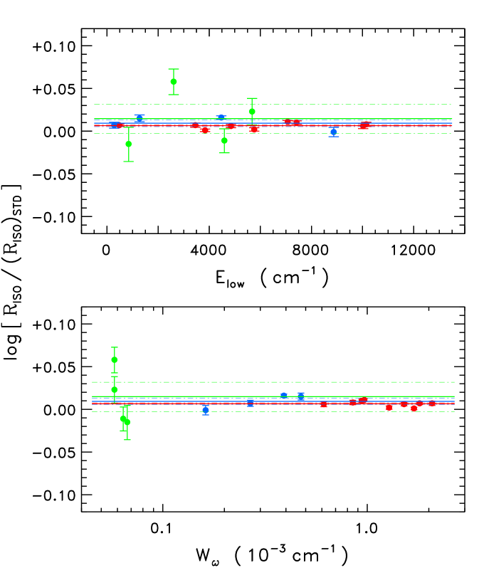
The second step in this part of the analysis was to examine the derived and oxygen abundances (e.g., from Fig. 5b) as a function of excitation energy, , and equivalent width, , to uncover any trends for the particular model. Figure 5c depicts the procedure for the same case illustrated in Figs. 5a and 5b (full 3D model, scale). One sees that the derived oxygen abundances (in lower portions of the panels) average just below 600 ppm; the ’s have a slight but systematic dependence on ; the and samples are separated; but neither group displays a significant trend with equivalent width.
Also included in Fig. 5c are analogous results for the FAL-C 1D model (upper portions of the panels), also using the scale, and with all the other assumptions the same (except that a depth-independent microturbulence parameter of 1.7 km s-1 was introduced so that the 1D profiles matched the observed line widths). Now, the derived oxygen abundances are much higher (e.g., APK); the excitation slope is much steeper; the and samples still are separated, and in the same sense as for the 3D model; but also the hybrids show increased scatter.
The slope of the versus distribution was measured by a linear least squares fit to the (more numerous and more diverse in energy) overtone sample, and an offset (specified by the ratio ) was inferred by forcing the (smaller) sample of fundamental lines to fit the same slope. As is clear from the figure, the main dependence is on rather than , consistent with the selection criterion designed to minimize inclusion of partially saturated lines (which would stand out in the part of the diagram as anomalous). Note that the scatter of individual values about the linear relations is small for the 3D model.
Figure 5d is similar to 5c, but now compares results from the baseline ( K) full 3D model to those of Goldilocks ( K) and MAX ( K), again for the scale. The model variants show a systematic increase in with ; a smooth change in the abundance/excitation slope from positive to negative; and a reversal of the and separation (and, of course, for the Goldilocks option). Significantly, the excitation slope is nearly zero for the Goldilocks case, an outcome that is not a foregone conclusion from simply forcing the and samples to agree.
Figure 6 summarizes the oxygen abundance exercises for snapshots A–C, provided separately for the independent oscillator strengths, G94 and HR96; the full 3D model for the scale; and the 1D model, also for the average -values.
Although the details differ between the different oscillator strength scales, the overall behavior is similar: the baseline models predict lower oxygen abundances, significant / slopes, and separated and distributions (dots mark the values), whereas the maximally-perturbed models yield higher oxygen abundances, more negative / slopes, and and separated in the opposite sense. The Goldilocks snapshots have intermediate values of and intermediate excitation slopes. A subtle consequence of the differences between the G94 and HR96 -values is on the balance temperatures (the mentioned earlier) to force for the different models. The G94 scale picks a lower balance temperature, typically closer to the baseline (), whereas HR96 picks a higher value, closer to the MAX option. Not surprisingly, the average -value scale selects intermediate balance temperatures. The effect on the balance temperatures is important given the highly temperature sensitive nature of the problem. Also note that the G94 “bow ties” scatter around zero excitation slope, whereas the HR96 symbols appear to be offset from the zero line. This could be taken as some support for the G94 scale over HR96 (although we will see later that other evidence points in the opposite direction).
The oxygen abundances of the baseline models (550–580 ppm) are higher than the “low” oxygen abundances (460–490 ppm) derived from atomic oxygen lines initially by Allende-Prieto, Lambert, & Asplund (2001) and subsequently Asplund et al. (2004), which originally inspired the so-called “Oxygen Crisis” conflict with helioseismology (e.g., APK; and references to previous work therein). In fact, the higher values from the “extreme” MAX perturbed snapshots fall around the ppm favored by helioseismology (e.g., Ayres 2008). The Goldilocks values are close to the intermediate range proposed in a more recent study of atomic oxygen by Caffau et al. (2008). Again, this comparison assumes that is exactly one-half : the inferred oxygen abundance would have to be modified to the extent that the true abundance ratio deviates from that value.
The 1D model illustrated here shows a starkly different behavior than the 3D snapshots (as anticipated in SAGS and APK): the inferred are much larger, and the excitation slopes are steeper. To the extent that shallow slopes indicate thermal harmony in the models, the 1D example clearly is far away from that ideal; almost certainly because it must represent at each pressure level the wide diversity of temperatures in the real inhomogeneous atmosphere by only a single compromise value. The spatial averages of ultraviolet and visible spectral diagnostics inherent in forming the 1D model clearly fail miserably to capture the average behavior of the CO and bands, undoubtedly because the UV/optical has a natural bias toward hotter temperatures, while molecules have the diametrically opposite bias. We can safely conclude that the CO problem is the gold-standard example where a 1D model provides a very misleading — in fact completely useless — viewpoint compared to 3D (as ventured earlier by SAGS).
As a tracer of the oxygen abundance, the CO bands clearly are very model dependent, and thus are more susceptible to systematic errors in the thermal properties of the 3D models than typical atomic lines. Personally we favor the Goldilocks scenario over the unperturbed baseline snapshots, or the MAX variants. We consider the latter to be an extreme case, for the reasons outlined earlier. At the same time, the baseline model very likely is slightly too cool compared with the real photosphere, by virtue of the additional heating process not currently included in the simulations. Thus our natural preference is for the intermediate Goldilocks case: not too cool, not too warm. Our discussion of the oxygen abundance here mainly is for sake of completeness, since we utilize essentially as a transfer standard, as cautioned earlier. Thankfully, the rather broad range of derived values has a smaller impact on the isotopic analysis, owing to its differential nature (although we will see that part of the anticipated cancellation is not realized owing to the influence of the different -value scales on the Goldilocks balance temperatures, which feeds back into the isotopic problem).
3.3 Isotopic Ratios
The final piece of the puzzle was to determine the isotopic ratios for the reference snapshots, the full 3D model, and their temperature-perturbed cousins, given the oxygen abundances and excitation slopes derived in the first phase.
Owing to the different molecular weights of the isotopic diatoms, not only are the rovibrational properties different, but so too is the chemistry. The dissociation potential, for example, is slightly affected by the different ground level energies of the isotopomers (Morton & Noreau 1994), as is the kinetic factor in the dissociative equilibrium. Furthermore, the partition functions of each isotopomer are affected by the slightly compressed rovibrational energy ladders (G94).
In the equation of state, we accounted for the ICE formation of the significant diatomic molecules in a solar mixture, based on Grevesse & Sauval (1998) abundances for all elements except O, which we varied; C, which we took as O; and N, which we set at O. In the ICE solution, for simplicity, we included only the dominant isotope of each element (e.g., 12C for carbon and 16O for oxygen), with the appropriate molecular formation parameters for that combination. This is a good approximation for CO because the contribution by the rare isotopes is only about 1%.
We then treated the CO isotopomer abundances as fractions of the total concentration obtained from the dominant-isotope ICE solution. To derive the relevant ratios, we simulated the full isotopic chemistry, but restricted to CO itself (and the main isotopomers 26, 27, 28, and 36; ignoring the minute concentrations of 37 and 38). We expressed the isotopomer abundance for, say, 13C16O, relative to the calculated total density as
| (1) |
where is the 13C16O number density, is the total CO density from the ICE solution, is the 12C/13C ratio, is the 16O/17O ratio, and so forth. The leading term in square brackets simply reflects the fraction of carbon that is 13C, and the trailing term in square brackets reflects the fraction of oxygen that is 16O. The product of the two would be the isotopomer abundance ratio if the chemistry were independent of the molecular weights and dissociation constants. Finally, is a correction factor, derived from the CO isotopomer network, which captures the impact of the more subtle chemistry issues. In practice, is temperature and density dependent, especially for K and high densities ( cm-3); and exhibits asymptotic behavior below 3500 K and above 5000 K. However, it also happens that the dominant altered factors in the dissociative equilibrium nearly cancel, so is close to one, differing from unity at most by only about half a percent in the worst {} case. That implies that the isotopomer chemistry is close to that of the parent CO, on a per molecule basis, which conveniently justifies the dominant-isotope approximation in the global ICE chemistry.
We calculated the ’s in detail for medium snapshot “B,” and determined representative values: 1.0010, 1.0007, 1.0016, and 1.000 for isotopomers 36, 28, 27, and 26 respectively. We introduced these as temperature- and density-independent constants in the isotopomer synthesis. This is reasonable because the peak of the CO density function occurs at temperatures much warmer than the low- limit where the maximum departures of from unity occur.
SAGS performed a similar type of analysis, although they also included the factor of the partition function that appears in the line opacity, together with the factor of the partition function in the dissociative equilibrium, because in principle the two cancel, at least if the molecular formation is completely unsaturated (in the sense that ; i.e., only a small amount of the free carbon and oxygen has associated into CO). We chose to retain the partition function factors explicitly, and separately, in the line opacity and chemical equilibrium to allow for partial saturation effects in the lower temperature overshooting convective plumes of the 3D models, which are not accommodated by the SAGS strategy. Furthermore, the SAGS “opacity scale factors” were derived taking the isotopomer oscillator strengths equal to those of the equivalent parent transitions. However, the isotopomer strengths on either the G94 or HR96 scales are 4% less than for the equivalent parent transition (for 36 and 28; e.g., Fig. 1c), leading to a systematic error of at least that magnitude (isotopic abundances underestimated, and isotopic ratios, , overstated), all else being equal.
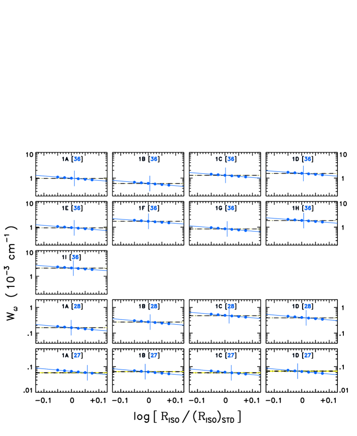
We adopted reference ’s of 90, 500, and 2650 for 23, 68, and 67, respectively (essentially the terrestrial standard values); then calculated equivalent widths for multiples (, as described earlier) of these, from 0.050 dex to +0.075 dex, in steps of 0.025 dex (six total). As we did for the oxygen abundances from the parent sample, we fitted a parabolic relation to the calculated equivalent widths and solved for the isotopic ratio scale factor that matched the observed . Figures 7a–c illustrate the procedure for the Goldilocks version of the full 3D model, utilizing the scale. We adopted a specific oxygen abundance, , for each simulation based on the sample, but adjusted the oscillator strengths of the isotopomer transitions (all type) by a multiplicative factor to compensate for any slope in versus :
| (2) |
where . The intercept, , and slope, , of the linear relation initially were derived from the sample, but then adjusted to according to the factor mentioned earlier; note also that . The -scaling of the -values simulates the effect of a gradient in the oxygen abundance with , at least in the regime where the CO formation is unsaturated.
Figure 7c shows that for the full 3D model Goldilocks option, and the average oscillator strengths, the isotopic abundance ratios 12C/13C and 16O/18O are slightly higher than terrestrial (by about 2%), with only small random errors due to the dispersion of values within each sample, particularly if we are permitted to describe these as standard errors of the mean. The 16O/17O ratio is slightly higher still, although now the dispersion among the four independent hybrid points is large, paralleling the large individual uncertainties. The 12C17O features are extremely weak, and therefore especially susceptible to errors in the local continuum level, so any conclusions drawn from that isotopomer will be much less secure than for the stronger 13C16O and 12C18O systems.
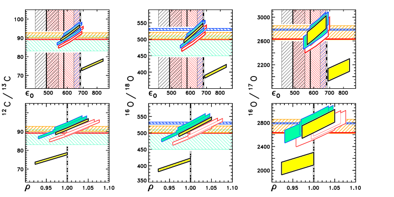
The derived isotopic ratios are depicted schematically in Figure 8, as a function of ( values) and the ratio described earlier, for the same set of models illustrated previously in Fig. 6.
On the G94 scale, the isotopic ratios are systematically % lower than those derived from the HR96 scale, for the baseline and MAX models. Going from the baselines to the MAX models, the isotope ratios increase systematically for both oscillator strength scales, by nearly same amount for each: 8% higher for 36 and 10% higher for 28 and 27. The dispersion in among the reference snapshots is 2–3% for the baselines, and about half that for the MAX variants (undoubtedly because the latter are closer together in temperature than the baselines thanks to the temperature-correction procedure).
On the G94 scale, the values are systematically % higher than those from the HR96 scale, for the baseline models and the MAX variants, due to the systematically slightly lower G94 -values. For the baseline models, the average is about 570 ppm with a 2.6% snapshot dispersion. For the MAX models, the dispersion shrinks to about 1%, again likely because of the temperature confluence effect, but the absolute oxygen abundance rises a dramatic 21% to about 685 ppm. The large increase in the derived oxygen abundance with only a small –110 K change from the baseline models demonstrates the strong temperature sensitivity of CO. Note, however, that the rise in the isotopic ratios from baseline to MAX is only about half that of the oxygen abundance itself, demonstrating some significant cancellations in the differential analysis.
Now consider the Goldilocks models that force the and parent samples to agree in oxygen abundance space. The differences between the results for the two oscillator strength scales are more pronounced, because the systematic offsets between the G94 and HR96 -values for and went in opposite directions (at least for the lower vibrational bands that are relevant in this analysis), so the balance temperature to force them into agreement was different. In fact, the HR96 Goldilocks temperatures are closer to the MAX values, averaging 50% of the maximum ’s; while the G94 temperatures are closer to the baselines: only 1 K higher in the case of snapshot “C,” and only 7 K higher for “B.” As before, the dispersions of the isotopic ratios among the three Goldilocks snapshots for a given oscillator strength scale are small (1%), but now the HR96 values are systematically higher by about 5–6% than those for G94. The average oxygen abundances are about 600 ppm for G94 and 630 ppm for HR96, with a small (2%) dispersion among the snapshots in both cases (although with snapshots “B” and “C” giving nearly identical results, but “A” almost 25 ppm higher).
We now are in a position to recommend isotopic ratios based on the global analysis. We choose the Goldilocks option as our preferred temperature correction, because these are the models that achieve agreement between the and bands. This would be the desired outcome for a model that has an optimum thermal structure as far as the molecules are concerned, if the oscillator strength scale is reliable. We chose recommended values from the full 3D model, and the average -values, because we have no reason (yet) to prefer one of the oscillator strength scales over the other. Further, within the set of reference snapshots we can identify the sources of uncertainty devolving from: (1) the reference oxygen abundances (small, contributed by the parameter derived from the ten hybrids); (2) “noise” in the isotopomer hybrid line samples (generally small, except for isotopomer 27); (3) variations among the snapshots (also small, when considering the full set of 16); and (4) differences imposed by the alternative oscillator strength scales (dominates the others). The first three sources can be characterized by standard errors of the mean, because we are comparing multiple realizations of ostensibly similar objects. For the oscillator strength scales, we have only two examples, so we quote the uncertainty as one-half the difference between the alternative results (equivalent to a 1 dispersion for a sample of two).
In addition, we can characterize the further uncertainty that arises from the reality that we do not know, a priori, which is the more correct 3D model scenario: baseline, Goldilocks, or MAX. This error must be treated as a standard deviation, because we are comparing ostensibly different objects. The derived “scenario uncertainty” typically is larger than any of the individual sources, and in fact is larger than all those collectively (quadratic sum), except again in the case of isotopomer 27, for which the sample random error is large and comparable to the scenario component.
We find:
| 12C/13C= | 91.4 | ||||||
|---|---|---|---|---|---|---|---|
| 16O/18O= | 511 | ||||||
| 16O/17O= | 2738 | ||||||
| = | 603 |
The first error (1 s.e.) is that associated with the uncertainty of the applied in the isotopomer synthesis, resulting from scaling the derived abundance (which has negligible random error owing to the large number of contributing overtone transitions and their generally small scatter) according to the factor. The % for the ten hybrid lines (1 s.e.%) is amplified for the isotopic ratios by a factor of (derived by numerical experiments). The second uncertainty (1 s.e.) is that due to the isotopomer sample random error (or the hybrid sample for ). The third (1 s.e.) is the snapshot variability, taking the dispersion of results from the three independent reference snapshots, for the scale, and dividing by to estimate the s.e. over the full 3D model. The fourth (1 ) is from the -values, as described above. Finally, the fifth (1 ) is the scenario uncertainty: i.e., which level of temperature correction, if any, should be applied to the baseline model. The leading error quoted in the trailing parentheses is the total uncertainty for the Goldilocks option treated alone, which is the “optimistic” value if we believe that Goldilocks is the most realistic of the scenarios. The second parenthetical error includes the scenario component, and thus would fall at the conservative, pessimistic, end of the uncertainty spectrum. Note that in all cases, the snapshot variability contribution is smaller than the total sample random error (sum of first two terms in quadrature), demonstrating that 16 snapshots is sufficient for the purpose.
Table 3 summarizes abundances and isotopic ratios derived with the three temperature correction scenarios applied to the full 3D model, for the scale; and the Goldilocks variants of the full model separately for the G94 and HR96 -values.
For comparison, we carried out the isotopic analysis using the FAL-C 1D model illustrated earlier. In this case, as with the 3D models, and for all three oscillator strength options, it also was necessary to impose a balance temperature to bring the and ’s into agreement. This was K for the scale. Note that because the 1D temperature stratification in a sense already is at the maximum level, owing to the UV/optical bias in its construction, the additional positive temperature enhancement is counterintuitive (and plainly unphysical, to the extent that 1D models can claim to be physical in the first place). Nevertheless, the results from the 1D model follow the pattern seen in 3D: the Goldilocks version yields a higher oxygen abundance than the baseline model by about 13%, while the isotopic ratios also are higher, but only about half of the corresponding rise.
The results for the 1D Goldilocks scenario with the average -values are as follows: ppm; 12C/13C=; 16O/18O=; and 16O/17O=. Although not directly comparable, these are similar to the 1D values obtained previously by APK, in the sense that the derived isotopic ratios all are significantly lower than terrestrial, while the inferred oxygen abundance is much higher than any contemporary-accepted value. The discouraging corollary is that all the previous efforts devoted to deriving abundances and isotopic ratios from 1D synthesis of CO, and other molecules, must be considered in vain, since it is clear that this particular problem is especially prone to the thermal differences between a 1D average temperature stratification versus the fluctuations inherent in a dynamically convecting late-type photosphere.
To be sure, the earlier Ayres et al. work made a concerted effort to incorporate temperature perturbations in a schematic way by considering a set of 1D multicomponent models that were scaled from a baseline thermal profile by depth-independent positive and negative increments in temperature, and weighted by a Gaussian-like distribution to mimic observed continuum brightness histograms. However, consideration of the different types of thermal structures populating a 3D snapshot (e.g., Ayres 2008: his Fig. 2), shows that convection does not simply raise and lower the temperature profile uniformly, but rather skews it so that those stratifications that are hot deep in tend to be cooler higher up, and vice versa (origin of the so-called “reversed granulation” pattern at high altitudes). That skewness likely has a fundamental impact on the CO problem, since the continuum forms in deeper layers, while the molecular absorptions form higher up. Furthermore, thanks to the Wedemeyer-Böhm & Rouppe van der Voort (2009) Hinode study, we now know that the amplitudes of thermal fluctuations in the photosphere are significantly larger than assumed by APK, who had appealed to ground-based granulation measurements (that apparently were more affected by stray light and the telescope point response profile than realized). Thus, the APK multicomponent strategy was, in effect, much closer to 1D than 3D.
We also note, with respect to the earlier SAGS study, which derived rather lower equivalent values of from CO666Although the authors cast their results in terms of the carbon abundance, they did adopt the previous Asplund et al. (2004) low oxygen abundance, and obtained a C/O ratio of about 0.5, consistent with what we use here., that the 3D snapshots utilized in that work apparently were somewhat cooler above than those employed here (see, e.g., Caffau et al. 2008, their Fig. 1). The cooler temperature profile likely was a consequence of the fewer-frequency opacity binning used in the earlier models. As we have seen here, cooler mid-photospheric temperatures tend to predict systematically lower oxygen abundances from CO and lower isotopic ratios, all else being equal (although, to be fair, the SAGS isotopic ratios are consistent with those derived here, given the large error bars of the earlier 3D study [Fig. 8]).
4 Discussion and Conclusions
The value (10, 23) [] derived from the ATMOS spectra is somewhat smaller of a deficit than the Genesis inferred photospheric value of 530 []. Our photospheric ratio implies a larger deficit [], closer to the Genesis result, although hardly any weight can be attached to this owing to the uncomfortably large measurement errors. Therefore our results, while tantalizing, cannot confirm that the solar photosphere falls 28 below the terrestrial fractionation line, as determined by Genesis (McKeegan et al. 2011). The value of (1.3, 3.3) [] measured here is similar to our and is slightly higher than the terrestrial value of 89.2. The main conclusion — given our intermediate modelization strategy and middle choice of oscillator strength scales — is that the photospheric isotopic ratios of carbon and oxygen are slightly on the high side of the terrestrial values, although not to the extent found by Genesis for the heavy oxygen isotopes. That the Sun likely is lighter than the Earth, isotopically speaking, means that exotic fractionation mechanisms need not be invoked for the early solar system, although the Genesis findings for and imply that whatever the process, it must have been mass-independent (McKeegan et al. 2011).
Taking some additional liberties, we can turn the problem around and ask what are the implications if Genesis is correct and the actual photospheric oxygen isotopic ratios are above the terrestrial standard values? If we further require that a satisfactory model must have , we see that this combination favors the HR96 -value scale (Fig. 8 and Table 3), and by implication , close to the Genesis heavy oxygen deficits; and one step further, an ppm well beyond the upper side of the “low-O” error flags, just at the lower edge of the seismic range.
In short, we reinforce the conclusions of Scott et al. that the solar CO problem is a poster child for the importance of 3D effects: the 1D models simply fail to account for key aspects of the highly temperature sensitive molecular formation, and provide completely misleading results in the end. We showed, moreover, that altering the thermal profiles of the 3D models slightly according to reasonable criteria can achieve a better match to the empirical CO spectra, but with an accompanying significant impact on especially the oxygen abundance. Although we again caution that CO is a less than ideal abundance indicator, and uncertainties remain due to the discordance between the available oscillator strength scales, the derived ’s for our favored “Goldilocks” scenario are in accord with the ‘high’ range found in recent 3D studies of solar atomic oxygen, and possibly within striking distance of a value that could be swallowed, without grimacing, by helioseismology.
References
- Abrams et al. (1999) Abrams, M. C., Goldman, A., Gunson, M. R., Rinsland, C. P., & Zander, R. 1999, Appl. Opt., 35, 2747
- Allende Prieto et al. (2001) Allende Prieto, C., Lambert, D. L., & Asplund, M. 2001, ApJ, 556, L63
- Asplund et al. (2004) Asplund, M., Grevesse, N., Sauval, A. J., Allende Prieto, C., & Kiselman, D. 2004, A&A, 417, 751
- Asplund et al. (2005) Asplund, M., Grevesse, N., & Sauval, A. J. 2005, Cosmic Abundances as Records of Stellar Evolution and Nucleosynthesis, 336, 25
- Asplund et al. (2000) Asplund, M., Nordlund, Å., Trampedach, R., Allende Prieto, C., & Stein, R. F. 2000, A&A, 359, 729
- Auer (1976) Auer, L. 1976, JQSRT, 16, 931
- Ayres (1975) Ayres, T. R. 1975, ApJ, 201, 799
- Ayres (2008) Ayres, T. R. 2008, ApJ, 686, 731
- Ayres et al. (2006) Ayres, T. R., Plymate, C., & Keller, C. U. 2006, ApJS, 165, 618 (APK)
- Ayres & Wiedemann (1989) Ayres, T. R., & Wiedemann, G. R. 1989, ApJ, 338, 1033
- Beeck et al. (2012) Beeck, B., Collet, R., Steffen, M., et al. 2012, A&A, 539, A121
- Burnett et al. (2003) Burnett, D. S., et al. 2003, Space Science Reviews, 105, 509
- Caffau et al. (2008) Caffau, E., Ludwig, H.-G., Steffen, M., et al. 2008, A&A, 488, 1031
- Clayton (2002) Clayton, R. N. 2002, Nature, 415, 860
- Dominguez (2010) Dominguez, G. 2010, ApJ, 713, L59
- Fontenla et al. (1993) Fontenla, J. M., Avrett, E. H., & Loeser, R. 1993, ApJ, 406, 319
- Freytag et al. (2012) Freytag, B., Steffen, M., Ludwig, H.-G., et al. 2012, Journal of Computational Physics, 231, 919
- Gonfiantini et al. (1994) Gonfiantini, R., Stichler, W., & Rozanski, K. 1995, IAEA-TECDOC-825 (Vienna: International Atomic Energy Agency), 13
- Goorvitch (1994) Goorvitch, D. 1994, ApJS, 95, 535 (G94)
- Grevesse & Sauval (1998) Grevesse, N., & Sauval, A. J. 1998, Space Science Reviews, 85, 161
- Grevesse et al. (2010) Grevesse, N., Asplund, M., Sauval, A. J., & Scott, P. 2010, Ap&SS, 328, 179 (GASS)
- Hall (1973) Hall, D. N. B. 1973, ApJ, 182, 977
- Hall et al. (1972) Hall, D. N. B., Noyes, R. W., & Ayres, T. R. 1972, ApJ, 171, 615
- Harris et al. (1987) Harris, M. J., Lambert, D. L., & Goldman, A. 1987, MNRAS, 224, 237
- Hashizume & Chaussidon (2005) Hashizume, K., & Chaussidon, M. 2005, Nature, 434, 619
- Holweger & Müller (1973) Holweger, H., & Müller, E. A. 1974, Sol. Phys., 39, 19
- Hure & Roueff (1996) Hure, J. M., & Roueff, E. 1996, A&AS, 117, 561 (HR96)
- Ireland et al. (2006) Ireland, T. R., Holden, P., Norman, M. D., & Clarke, J. 2006, Nature, 440, 776
- Krot et al. (2005) Krot, A. N., et al. 2005, ApJ, 622, 1333
- Krot et al. (2010) Krot, A. N., Nagashima, K., Ciesla, F. J., et al. 2010, ApJ, 713, 1159
- Langer & Penzias (1993) Langer, W. D., & Penzias, A. A. 1993, ApJ, 408, 539
- Lee et al. (2008) Lee, J.-E., Bergin, E. A., & Lyons, J. R. 2008, Meteoritics and Planetary Science, 43, 1351
- Lenz & Ayres (1992) Lenz, D. D., & Ayres, T. R. 1992, PASP, 104, 1104
- Lyons & Young (2005) Lyons, J. R., & Young, E. D. 2005, Nature, 435, 317
- McKeegan et al. (2011) McKeegan, K. D., Kallio, A. P. A., Heber, V. S., et al. 2011, Science, 332, 1528
- Morton & Noreau (1994) Morton, D. C., & Noreau, L. 1994, ApJS, 95, 301
- Sakamoto et al. (2007) Sakamoto, N., Seto, Y., Itoh, S., et al. 2007, Science, 317, 231
- Scott et al. (2006) Scott, P. C., Asplund, M., Grevesse, N., & Sauval, A. J. 2006, A&A, 456, 675 (SAGS)
- Sheffer et al. (2002) Sheffer, Y., Lambert, D. L., & Federman, S. R. 2002, ApJ, 574, L171
- Smith et al. (2009) Smith, R. L., Pontoppidan, K. M., Young, E. D., Morris, M. R., & van Dishoeck, E. F. 2009, ApJ, 701, 163
- Stein (2012) Stein, R. F. 2012, Living Reviews in Solar Physics, 9, 4
- Ulmschneider (1974) Ulmschneider, P. 1974, Sol. Phys., 39, 327
- Wedemeyer-Böhm et al. (2005) Wedemeyer-Böhm, S., Kamp, I., Bruls, J., & Freytag, B. 2005, A&A, 438, 1043
- Wedemeyer-Böhm & Rouppe van der Voort (2009) Wedemeyer-Böhm, S., & Rouppe van der Voort, L. 2009, A&A, 503, 225
- Wiens et al. (1997) Wiens, R. C., Burnett, D. S., & Huss, G. R. 1997, Lunar and Planetary Institute Conference Abstracts, 28, 1553
- Wiens et al. (2004) Wiens, R. C., Burnett, D. S., McKeegan, K. D., Thiemens, M. H., Franchi, I. A., Bochsler, P., & Mao, P. 2004, Lunar and Planetary Institute Conference Abstracts, 35, 1296
- Woods (2009) Woods, P. M. 2009, arXiv:0901.4513
- Yurimoto & Kuramoto (2004) Yurimoto, H., & Kuramoto, K. 2004, Science, 305, 1763
| Transition | FWHM | Flag | ||||
|---|---|---|---|---|---|---|
| (cm-1) | (cm-1) | ( cm-1) | (km s-1) | |||
| 2–1 P92 | 1638.5309 | 17997.97 | 4.44 | n | ||
| 2–1 P91 | 1644.9269 | 17666.30 | 4.56 | n | ||
| 2–1 P90 | 1651.3006 | 17337.83 | 4.50 | n | ||
| 2–1 P89 | 1657.6517 | 17012.59 | 4.51 | n | ||
| 1A26 | 1648.8911 | 17464.58 | 4.54 | |||
| 1–0 P94 | 1648.8738 | 16683.95 | 4.36 | n | ||
| 1–0 P93 | 1655.3485 | 16342.62 | 4.41 | l | ||
| 1–0 P92 | 1661.8011 | 16004.50 | 4.50 | l | ||
| 1B26 | 1655.7844 | 16321.21 | 4.44 | |||
| 1–0 P90 | 1674.6395 | 15337.95 | 4.49 | n | ||
| 1–0 P89 | 1681.0251 | 15009.55 | 4.55 | l | ||
| 1–0 P87 | 1693.7284 | 14362.57 | 4.61 | n | ||
| 1–0 P86 | 1700.0458 | 14044.01 | 4.61 | l | ||
| 1C26 | 1688.8924 | 14613.11 | 4.60 | |||
| 3–2 P82 | 1677.9226 | 16824.71 | 4.75 | n | ||
| 4–3 P76 | 1690.6726 | 17085.25 | 4.83 | l | ||
| 5–4 P71 | 1696.4065 | 17725.30 | 4.74 | r | ||
| 5–4 P70 | 1702.2023 | 17470.95 | 4.76 | n | ||
| 1D26 | 1692.2540 | 17285.70 | 4.80 | |||
| 2–1 P85 | 1682.8292 | 15744.06 | 4.68 | n | ||
| 2–1 P84 | 1689.0661 | 15435.10 | 4.72 | n | ||
| 2–1 P83 | 1695.2798 | 15129.43 | 4.78 | r | ||
| 2–1 P82 | 1701.4702 | 14827.07 | 4.79 | n | ||
| 1E26 | 1692.8647 | 15250.59 | 4.77 | |||
| 9–8 P28 | 1820.8624 | 17851.92 | 4.65 | n | ||
| 9–8 P22 | 1847.1185 | 17308.93 | 4.56 | n | ||
| 9–8 P20 | 1855.6181 | 17156.12 | 4.61 | l | ||
| 1F26 | 1840.6961 | 17451.14 | 4.63 | |||
| 8–7 P8 | 1929.5857 | 14578.75 | 4.47 | n | ||
| 8–7 P7 | 1933.4265 | 14549.96 | 4.46 | r | ||
| 8–7 R5 | 1980.2139 | 14503.17 | 4.41 | n | ||
| 8–7 R6 | 1983.5660 | 14524.77 | 4.46 | n | ||
| 1G26 | 1955.6292 | 14541.29 | 4.47 | |||
| 7–6 P5 | 1966.8906 | 12518.28 | 4.52 | n | ||
| 7–6 P4 | 1970.6641 | 12500.11 | 4.40 | n | ||
| 7–6 R3 | 1999.6015 | 12485.57 | 4.39 | l | ||
| 7–6 R4 | 2003.0602 | 12500.11 | 4.53 | b | ||
| 1H26 | 1985.3169 | 12501.79 | 4.49 | |||
| 6–5 P2 | 2004.1715 | 10463.23 | 4.37 | n | ||
| 5–4 R0 | 2041.4229 | 8414.46 | 4.33 | l | ||
| 1I26 | 2021.0742 | 9539.74 | 4.37 | |||
| 4–3 R0 | 2067.7353 | 6350.43 | 4.49 | n | ||
| 1J26 | 2067.7353 | 6350.43 | 4.49 | |||
| 7–5 P63 | 3635.1206 | 17751.86 | 4.35 | n | ||
| 7–5 P62 | 3642.8485 | 17526.74 | 4.23 | n | ||
| 8–6 P54 | 3652.1604 | 17807.96 | 4.21 | r | ||
| 9–7 P43 | 3676.6781 | 17832.96 | 4.15 | n | ||
| 9–7 P42 | 3683.0854 | 17680.10 | 4.36 | l | ||
| 2A26 | 3659.7804 | 17723.43 | 4.28 | |||
| 8–6 P42 | 3733.6516 | 15726.29 | 4.05 | l | ||
| 8–6 P41 | 3740.0303 | 15575.43 | 4.24 | r | ||
| 9–7 P25 | 3782.1151 | 15616.62 | 4.21 | l | ||
| 9–7 P22 | 3797.6212 | 15358.43 | 4.34 | r | ||
| 2B26 | 3761.0750 | 15576.80 | 4.23 | |||
| 7–5 P34 | 3833.8782 | 12627.24 | 4.25 | n | ||
| 7–5 P32 | 3845.6079 | 12383.19 | 4.34 | r | ||
| 7–5 P29 | 3862.7120 | 12044.06 | 4.21 | n | ||
| 7–5 P25 | 3884.5963 | 11642.40 | 4.31 | l | ||
| 2C26 | 3857.0982 | 12167.44 | 4.28 | |||
| 6–4 P35 | 3879.0270 | 10738.94 | 4.26 | r | ||
| 6–4 P34 | 3885.0247 | 10610.31 | 4.27 | n | ||
| 6–4 P33 | 3890.9573 | 10485.30 | 4.28 | r | ||
| 2D26 | 3885.0686 | 10610.17 | 4.25 | |||
| 9–7 R15 | 3940.7097 | 14880.83 | 4.36 | n | ||
| 9–7 R17 | 3945.4187 | 14999.42 | 4.31 | b | ||
| 9–7 R18 | 3947.6644 | 15064.07 | 4.19 | l | ||
| 2E26 | 3944.7547 | 14985.55 | 4.27 | |||
| 5–3 P35 | 3930.2825 | 8696.96 | 4.15 | r | ||
| 5–3 P34 | 3936.3153 | 8567.10 | 4.26 | l | ||
| 5–3 P33 | 3942.2830 | 8440.90 | 4.32 | l | ||
| 5–3 P30 | 3959.7946 | 8084.27 | 4.49 | l | ||
| 5–3 P27 | 3976.7156 | 7760.68 | 4.26 | r | ||
| 5–3 P26 | 3982.2240 | 7660.18 | 4.25 | b | ||
| 2F26 | 3955.2330 | 8189.89 | 4.30 | |||
| 2–0 P50 | 3985.0994 | 4862.74 | 4.23 | n | ||
| 2–0 P49 | 3992.1960 | 4673.53 | 4.25 | r | ||
| 2–0 P48 | 3999.2296 | 4488.00 | 4.26 | r | ||
| 2G26 | 3992.3851 | 4669.23 | 4.29 | |||
| 3–1 P42 | 3988.6813 | 5563.81 | 4.35 | n | ||
| 3–1 P40 | 4001.7259 | 5251.07 | 4.20 | l | ||
| 3–1 P38 | 4014.5138 | 4953.09 | 4.23 | l | ||
| 3–1 P36 | 4027.0438 | 4669.91 | 4.21 | l | ||
| 2H26 | 4008.8637 | 5089.47 | 4.23 | |||
| 9–7 R29 | 3967.5315 | 16010.58 | 4.14 | r | ||
| 9–7 R30 | 3968.8942 | 16117.92 | 4.33 | n | ||
| 7–5 R61 | 4081.9755 | 17305.01 | 4.28 | l | ||
| 7–5 R60 | 4082.9238 | 17086.66 | 4.44 | n | ||
| 2I26 | 4025.4474 | 16626.88 | 4.30 | |||
| 7–5 R20 | 4057.6387 | 11221.85 | 4.29 | n | ||
| 7–5 R22 | 4061.7586 | 11379.17 | 4.38 | l | ||
| 7–5 R23 | 4063.7085 | 11463.29 | 4.28 | n | ||
| 2J26 | 4061.1143 | 11357.84 | 4.29 | |||
| 7–5 R29 | 4073.8593 | 12044.06 | 4.54 | r | ||
| 7–5 R33 | 4079.1405 | 12503.42 | 4.35 | n | ||
| 7–5 R37 | 4083.2217 | 13020.18 | 4.37 | n | ||
| 2K26 | 4078.7026 | 12518.27 | 4.41 | |||
| 3–1 P25 | 4091.2978 | 3378.95 | 4.34 | n | ||
| 3–1 P22 | 4107.4365 | 3105.64 | 4.24 | n | ||
| 3–1 P18 | 4128.0192 | 2794.07 | 4.26 | l | ||
| 3–1 P17 | 4132.9968 | 2725.63 | 4.32 | n | ||
| 2L26 | 4114.0663 | 3014.95 | 4.28 | |||
| 6–4 R72 | 4121.1779 | 17982.98 | 4.27 | n | ||
| 6–4 R70 | 4124.6822 | 17470.95 | 4.25 | l | ||
| 6–4 R67 | 4129.3348 | 16728.00 | 4.30 | l | ||
| 2M26 | 4125.4780 | 17331.22 | 4.27 | |||
| 6–4 R26 | 4122.3991 | 9711.92 | 4.30 | l | ||
| 6–4 R28 | 4125.7047 | 9914.68 | 4.33 | n | ||
| 6–4 R30 | 4128.7133 | 10132.02 | 4.30 | n | ||
| 6–4 R31 | 4130.1058 | 10246.15 | 4.34 | n | ||
| 2N26 | 4126.7659 | 10003.51 | 4.31 | |||
| 6–4 R36 | 4135.9451 | 10871.18 | 4.34 | n | ||
| 6–4 R37 | 4136.8872 | 11007.03 | 4.36 | r | ||
| 6–4 R39 | 4138.5446 | 11289.53 | 4.33 | n | ||
| 6–4 R40 | 4139.2596 | 11436.17 | 4.31 | n | ||
| 2O26 | 4137.6319 | 11146.33 | 4.34 | |||
| 5–3 R27 | 4177.5502 | 7760.68 | 4.32 | n | ||
| 5–3 R28 | 4179.2008 | 7864.86 | 4.39 | l | ||
| 5–3 R29 | 4180.7772 | 7972.73 | 4.32 | n | ||
| 5–3 R30 | 4182.2791 | 8084.27 | 4.33 | l | ||
| 5–3 R33 | 4186.3371 | 8440.90 | 4.37 | r | ||
| 5–3 R35 | 4188.6677 | 8696.96 | 4.31 | n | ||
| 2P26 | 4182.4733 | 8136.71 | 4.34 | |||
| 5–3 R69 | 4181.2480 | 15240.46 | 4.39 | n | ||
| 5–3 R68 | 4182.7632 | 14990.39 | 4.29 | n | ||
| 5–3 R66 | 4185.5532 | 14500.46 | 4.31 | n | ||
| 5–3 R65 | 4186.8282 | 14260.61 | 4.37 | l | ||
| 2Q26 | 4184.2968 | 14713.50 | 4.34 | |||
| 4–2 R73 | 4229.6013 | 14278.71 | 4.49 | l | ||
| 4–2 R72 | 4231.4032 | 14012.58 | 4.23 | l | ||
| 4–2 R69 | 4236.3246 | 13234.62 | 4.20 | r | ||
| 4–2 R68 | 4237.8042 | 12982.14 | 4.43 | l | ||
| 2R26 | 4234.2155 | 13559.28 | 4.32 | |||
| 4–2 R27 | 4231.1521 | 5683.53 | 4.35 | l | ||
| 4–2 R28 | 4232.8376 | 5788.69 | 4.36 | r | ||
| 4–2 R31 | 4237.4479 | 6126.46 | 4.43 | n | ||
| 4–2 R32 | 4238.8355 | 6246.46 | 4.32 | n | ||
| 2S26 | 4235.0904 | 5962.72 | 4.37 | |||
| 4–2 R66 | 4240.5231 | 12487.48 | 4.62 | l | ||
| 4–2 R65 | 4241.7626 | 12245.32 | 4.40 | r | ||
| 4–2 R64 | 4242.9224 | 12006.63 | 4.32 | n | ||
| 4–2 R63 | 4244.0026 | 11771.41 | 4.28 | n | ||
| 4–2 R62 | 4245.0034 | 11539.67 | 4.26 | n | ||
| 2T26 | 4242.9628 | 11984.87 | 4.36 | |||
| 4–2 R35 | 4242.5487 | 6628.63 | 4.39 | l | ||
| 4–2 R36 | 4243.6361 | 6763.39 | 4.35 | n | ||
| 4–2 R37 | 4244.6480 | 6901.83 | 4.34 | l | ||
| 4–2 R39 | 4246.4450 | 7189.72 | 4.43 | l | ||
| 4–2 R40 | 4247.2298 | 7339.16 | 4.31 | r | ||
| 4–2 R41 | 4247.9386 | 7492.25 | 4.34 | n | ||
| 2U26 | 4245.3507 | 7043.10 | 4.37 | |||
| 3–1 R17 | 4263.6356 | 2725.63 | 4.27 | r | ||
| 3–1 R18 | 4266.0904 | 2794.07 | 4.29 | n | ||
| 3–1 R19 | 4268.4725 | 2866.29 | 4.29 | n | ||
| 3–1 R20 | 4270.7816 | 2942.30 | 4.28 | n | ||
| 3–1 R21 | 4273.0177 | 3022.08 | 4.35 | l | ||
| 3–1 R22 | 4275.1805 | 3105.64 | 4.31 | n | ||
| 3–1 R23 | 4277.2699 | 3192.98 | 4.31 | l | ||
| 2V26 | 4270.9033 | 2958.84 | 4.30 | |||
| 3–1 R82 | 4265.4063 | 14827.07 | 4.36 | n | ||
| 3–1 R81 | 4267.9059 | 14528.02 | 4.23 | l | ||
| 3–1 R80 | 4270.3235 | 14232.31 | 4.03 | r | ||
| 3–1 R78 | 4274.9127 | 13650.91 | 4.30 | l | ||
| 3–1 R77 | 4277.0847 | 13365.25 | 4.13 | r | ||
| 2W26 | 4271.7245 | 14039.34 | 4.19 | |||
| 3–1 R66 | 4295.6311 | 10448.09 | 4.26 | n | ||
| 3–1 R65 | 4296.8351 | 10203.62 | 4.28 | n | ||
| 3–1 R64 | 4297.9594 | 9962.65 | 4.23 | b | ||
| 2X26 | 4296.8517 | 10195.79 | 4.27 | |||
| 2–0 R13 | 4306.4749 | 349.69 | 4.25 | n | ||
| 2–0 R14 | 4309.2544 | 403.46 | 4.35 | l | ||
| 2–0 R16 | 4314.5966 | 522.47 | 4.27 | n | ||
| 2–0 R17 | 4317.1590 | 587.72 | 4.30 | r | ||
| 2Y26 | 4312.2073 | 473.25 | 4.29 | |||
| 2–0 R20 | 4324.4098 | 806.38 | 4.30 | n | ||
| 2–0 R21 | 4326.6808 | 886.90 | 4.36 | r | ||
| 2–0 R22 | 4328.8785 | 971.23 | 4.27 | n | ||
| 2–0 R23 | 4331.0029 | 1059.37 | 4.26 | n | ||
| 2–0 R24 | 4333.0537 | 1151.31 | 4.29 | l | ||
| 2–0 R25 | 4335.0309 | 1247.05 | 4.25 | n | ||
| 2Z26 | 4329.9746 | 1025.69 | 4.29 |
Note. — Line center frequencies, , and lower level energies, , are from G94; -values are averages of G94 and HR96. Uncertainties on equivalent widths, , are 1 , based on Lenz & Ayres (1992), with an empirical estimate of the photometric noise. Rightmost column (“Flag”) indicates how profile was trimmed before the coaddition step: “n”– no trimming; “l”– left wing trimmed; “r”– right wing; “b”– both wings.
| Transition | FWHM | Flag | ||||
|---|---|---|---|---|---|---|
| (cm-1) | (cm-1) | ( cm-1) | (km s-1) | |||
| 13C16O | ||||||
| 2–1 P53 | 1835.8986 | 7263.82 | 3.97 | l | ||
| 2–1 P52 | 1841.0593 | 7074.05 | 4.21 | n | ||
| 2–1 P51 | 1846.1940 | 6887.74 | 4.02 | n | ||
| 1A36 | 1841.2046 | 7069.78 | 4.14 | |||
| 5–4 P36 | 1847.9960 | 10583.74 | 4.08 | n | ||
| 5–4 P32 | 1866.2495 | 10098.20 | 4.32 | r | ||
| 5–4 P29 | 1879.6415 | 9770.51 | 4.18 | l | ||
| 5–4 P28 | 1884.0480 | 9668.24 | 4.08 | n | ||
| 1B36 | 1869.8756 | 10022.02 | 4.14 | |||
| 2–1 P45 | 1876.4530 | 5842.88 | 4.16 | r | ||
| 2–1 P44 | 1881.4034 | 5680.97 | 4.03 | l | ||
| 1C36 | 1878.9695 | 5760.63 | 4.14 | |||
| 2–1 P40 | 1900.9348 | 5068.49 | 4.25 | r | ||
| 2–1 P37 | 1915.2963 | 4646.21 | 4.06 | l | ||
| 1D36 | 1908.3619 | 4850.57 | 4.14 | |||
| 4–3 P30 | 1899.3493 | 7871.16 | 4.04 | l | ||
| 4–3 P26 | 1917.0482 | 7465.37 | 4.01 | r | ||
| 4–3 P23 | 1930.0159 | 7198.08 | 4.07 | n | ||
| 4–3 P22 | 1934.2794 | 7116.07 | 4.18 | n | ||
| 1E36 | 1919.9709 | 7418.37 | 4.14 | |||
| 2–1 P34 | 1929.4078 | 4255.87 | 4.09 | l | ||
| 2–1 P33 | 1934.0555 | 4132.88 | 4.05 | n | ||
| 2–1 P30 | 1947.8280 | 3785.33 | 4.14 | n | ||
| 2–1 P28 | 1956.8665 | 3571.53 | 4.19 | n | ||
| 2–1 P27 | 1961.3423 | 3470.01 | 4.14 | n | ||
| 1F36 | 1946.1313 | 3838.53 | 4.14 | |||
| 5–4 R27 | 2080.6760 | 9569.47 | 4.09 | l | ||
| 5–4 R30 | 2088.1925 | 9876.26 | 4.07 | r | ||
| 5–4 R35 | 2099.9808 | 10457.16 | 4.26 | l | ||
| 5–4 R37 | 2104.4344 | 10713.78 | 4.17 | l | ||
| 1G36 | 2093.1762 | 10145.43 | 4.14 | |||
| 1–0 R12 | 2140.8278 | 286.58 | 3.99 | r | ||
| 1–0 R14 | 2147.2045 | 385.72 | 4.27 | l | ||
| 1–0 R17 | 2156.5089 | 561.89 | 4.17 | l | ||
| 1–0 R18 | 2159.5403 | 627.93 | 4.06 | l | ||
| 1H36 | 2151.8492 | 480.27 | 4.14 | |||
| 1–0 R42 | 2221.4090 | 3301.16 | 4.15 | n | ||
| 1–0 R43 | 2223.5190 | 3457.45 | 4.18 | r | ||
| 1–0 R44 | 2225.5905 | 3617.29 | 4.15 | r | ||
| 1I36 | 2223.4707 | 3455.82 | 4.14 | |||
| 12C18O | ||||||
| 3–2 P53 | 1809.5808 | 9260.84 | 4.27 | r | ||
| 3–2 P50 | 1824.8215 | 8709.06 | 4.36 | n | ||
| 3–2 P49 | 1829.8500 | 8531.98 | 4.86 | l | ||
| 4–3 P42 | 1840.5850 | 9401.32 | 3.74 | n | ||
| 4–3 P36 | 1868.8777 | 8564.81 | 4.12 | l | ||
| 1A28 | 1835.4927 | 8869.81 | 4.14 | |||
| 1–0 P15 | 2033.8515 | 439.11 | 4.36 | l | ||
| 1–0 P11 | 2050.0805 | 241.59 | 4.16 | n | ||
| 1–0 R9 | 2126.9299 | 164.74 | 3.80 | r | ||
| 1–0 R11 | 2133.4895 | 241.59 | 4.49 | r | ||
| 1B28 | 2084.7945 | 281.80 | 4.14 | |||
| 1–0 R22 | 2167.0986 | 925.05 | 3.91 | b | ||
| 1–0 R26 | 2178.2619 | 1282.61 | 4.07 | r | ||
| 1–0 R29 | 2186.2556 | 1588.75 | 3.82 | l | ||
| 1C28 | 2177.4391 | 1272.49 | 4.14 | |||
| 2–1 R37 | 2179.5029 | 4632.65 | 4.15 | r | ||
| 1–0 R48 | 2229.1062 | 4275.82 | 4.19 | n | ||
| 1–0 R49 | 2230.9793 | 4452.65 | 4.33 | n | ||
| 1D28 | 2209.7509 | 4472.02 | 4.14 | |||
| 12C17O | ||||||
| 1–0 P42 | 1931.5996 | 3365.44 | 4.38 | r | ||
| 1–0 P35 | 1966.0712 | 2351.97 | 6.71 | n | ||
| 1–0 P34 | 1970.8816 | 2221.79 | 3.49 | l | ||
| 1A27 | 1957.6087 | 2607.09 | 4.14 | |||
| 1–0 P50 | 1890.5340 | 4740.88 | 4.88 | n | ||
| 1–0 P49 | 1895.7624 | 4556.38 | 2.42 | n | ||
| 2–1 P37 | 1931.8009 | 4715.92 | 4.02 | l | ||
| 2–1 P34 | 1946.2171 | 4318.04 | 3.56 | n | ||
| 2–1 P33 | 1950.9647 | 4192.67 | 2.53 | r | ||
| 3–2 P20 | 1984.9124 | 4978.67 | 3.49 | l | ||
| 3–2 P16 | 2001.9015 | 4706.90 | 4.38 | l | ||
| 2–1 R37 | 2205.3932 | 4715.92 | 2.70 | l | ||
| 1B27 | 1991.2737 | 4592.26 | 4.14 | |||
| 2–1 P47 | 1881.9118 | 6276.42 | 6.46 | l | ||
| 2–1 P42 | 1907.2048 | 5451.32 | 2.31 | l | ||
| 3–2 P33 | 1926.3298 | 6264.26 | 8.32 | r | ||
| 3–2 P21 | 1980.5875 | 5055.74 | 2.30 | n | ||
| 2–1 R42 | 2216.4885 | 5451.32 | 5.24 | b | ||
| 1C27 | 2002.3517 | 5677.56 | 4.14 | |||
| 1–0 P29 | 1994.4960 | 1625.94 | 3.60 | b | ||
| 1–0 P24 | 2017.3692 | 1122.28 | 5.44 | l | ||
| 1–0 P21 | 2030.7301 | 864.53 | 3.67 | n | ||
| 1–0 P15 | 2056.6177 | 449.41 | 4.88 | l | ||
| 1–0 R7 | 2145.0538 | 104.92 | 5.48 | l | ||
| 1–0 R9 | 2151.8983 | 168.60 | 4.25 | l | ||
| 1D27 | 2052.3259 | 844.97 | 4.14 | |||
Note. — Line center frequencies, , and lower level energies, , are from G94; -values are averages of G94 and HR96. Uncertainties on equivalent widths, , are 1 , based on Lenz & Ayres (1992), with an empirical estimate of the photometric noise. Rightmost column (“Flag”) indicates how profile was trimmed before the coaddition step: “n”– no trimming; “l”– left wing trimmed; “r”– right wing; “b”– both wings. A uniform FWHM= 4.14 km s-1 was imposed in the Gaussian fitting procedure.
| Scenario | |||||||
|---|---|---|---|---|---|---|---|
| Average -values | |||||||
| B | 0 | 572 6 | 0.972 0.013 | 88.9 0.7 (0.2) | 493 7 ( 3) | 2642 204 (102) | |
| G | +34 | 603 6 | 1.000 0.011 | 91.4 0.7 (0.2) | 511 9 ( 4) | 2738 209 (104) | |
| M | +90 | 644 9 | 1.050 0.017 | 96.2 0.9 (0.3) | 544 10 ( 5) | 2915 203 (101) | |
| G94 -values | |||||||
| G | +17 | 587 7 | 1.000 0.014 | 89.3 0.9 (0.3) | 496 7 ( 3) | 2657 209 (104) | |
| HR96 -values | |||||||
| G | +51 | 620 7 | 1.000 0.010 | 93.7 0.8 (0.3) | 528 11 ( 5) | 2829 210 (105) | |
Note. — “Scenario” corresponds to one of three temperature correction schemes, parametrized by (in K): “B”= baseline; “G”= Goldilocks; and “M”= MAX. Abundance gradient, , is in units of ppm per cm-1. In (ppm) and columns, values refer to parent sample; corresponding values can be obtained by multiplying by factor. In and columns, cited uncertainties are 1 dispersions. In columns, first uncertainty is a 1 dispersion, second is 1 s.e.
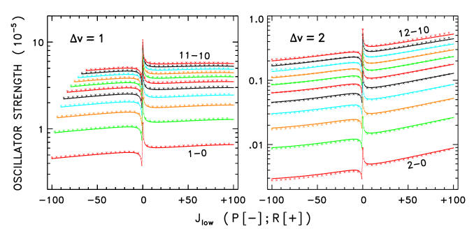
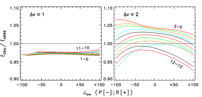
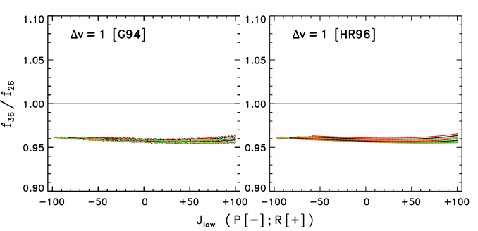
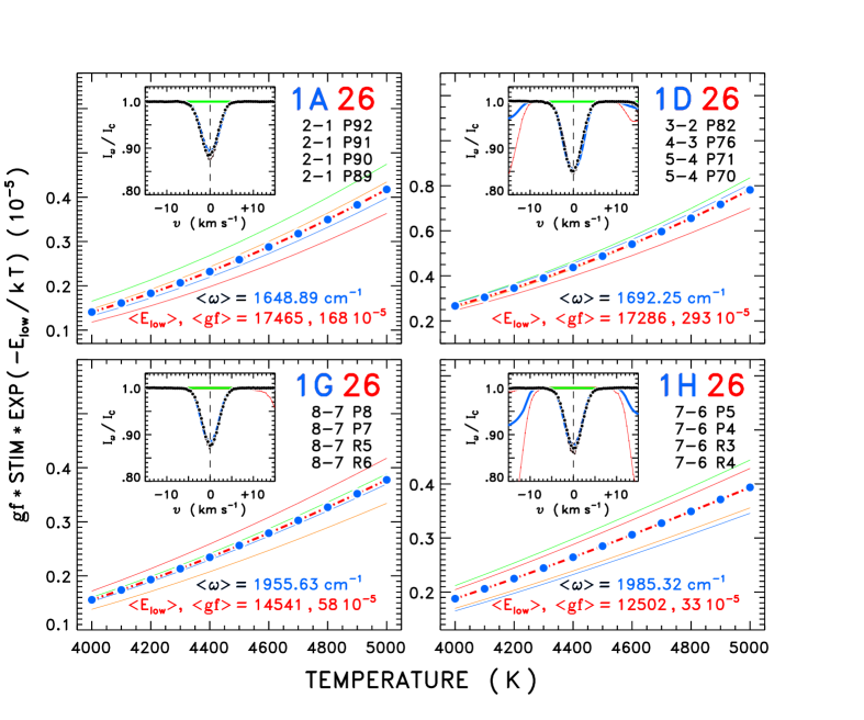
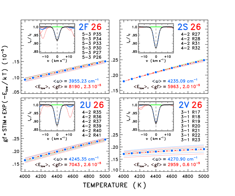
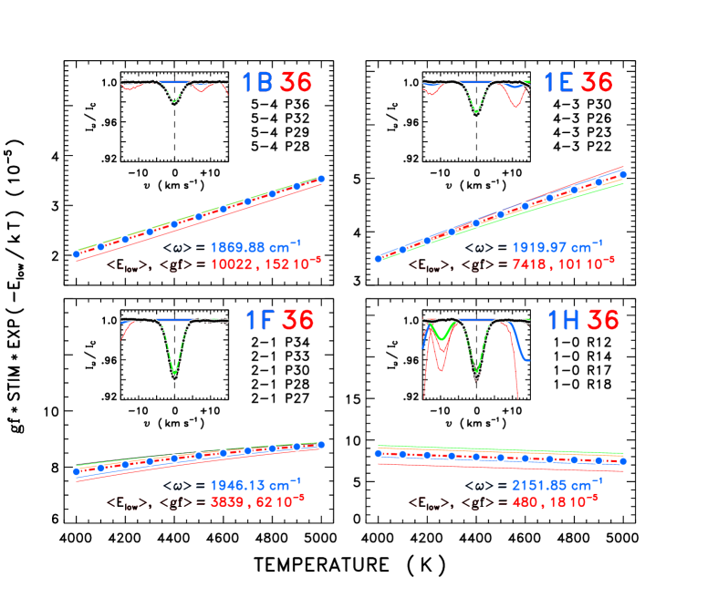
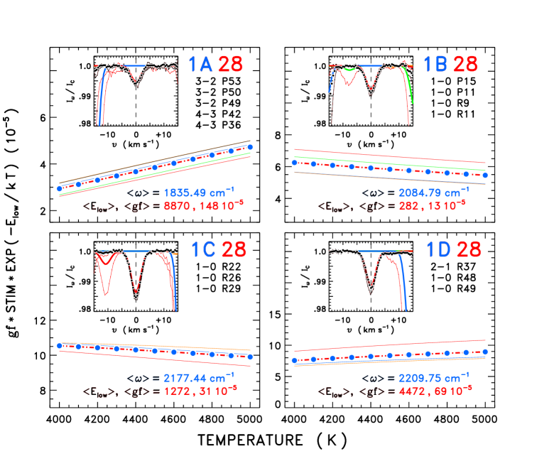
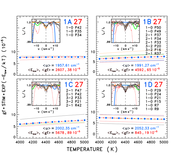
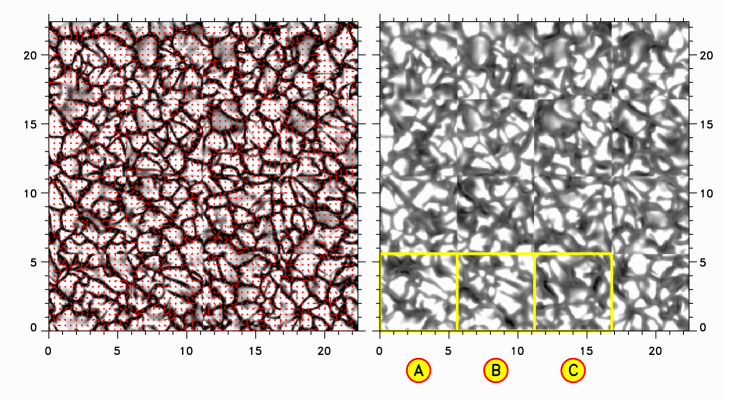
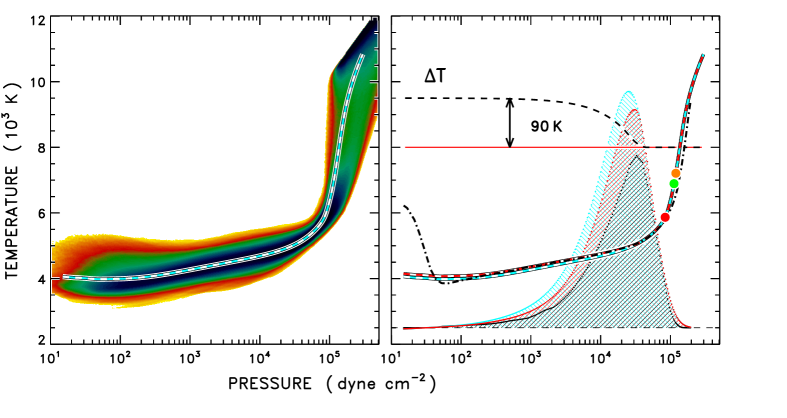
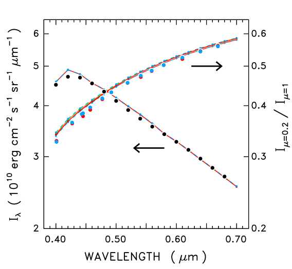
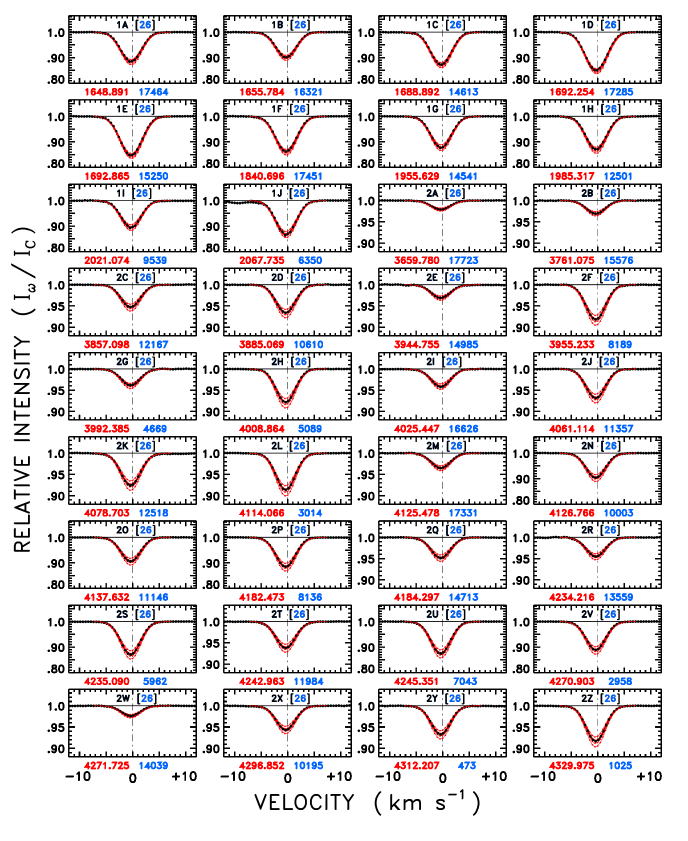
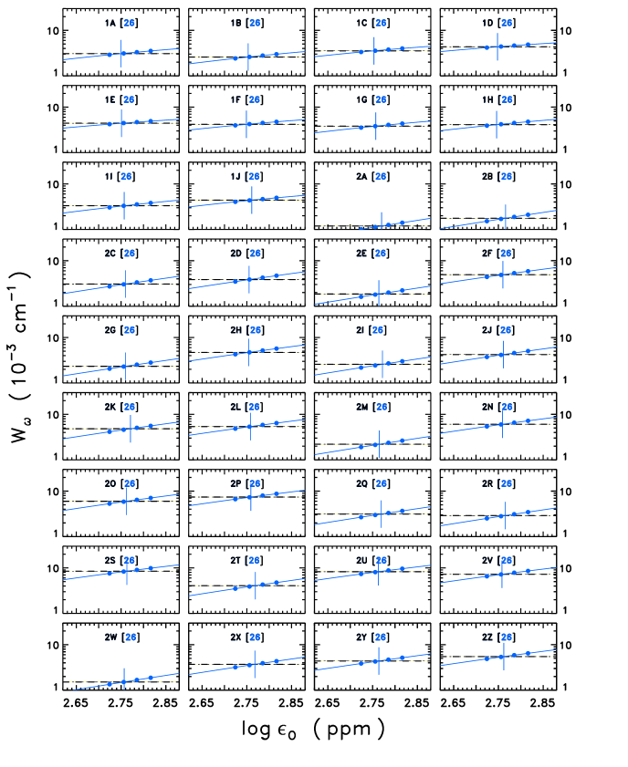
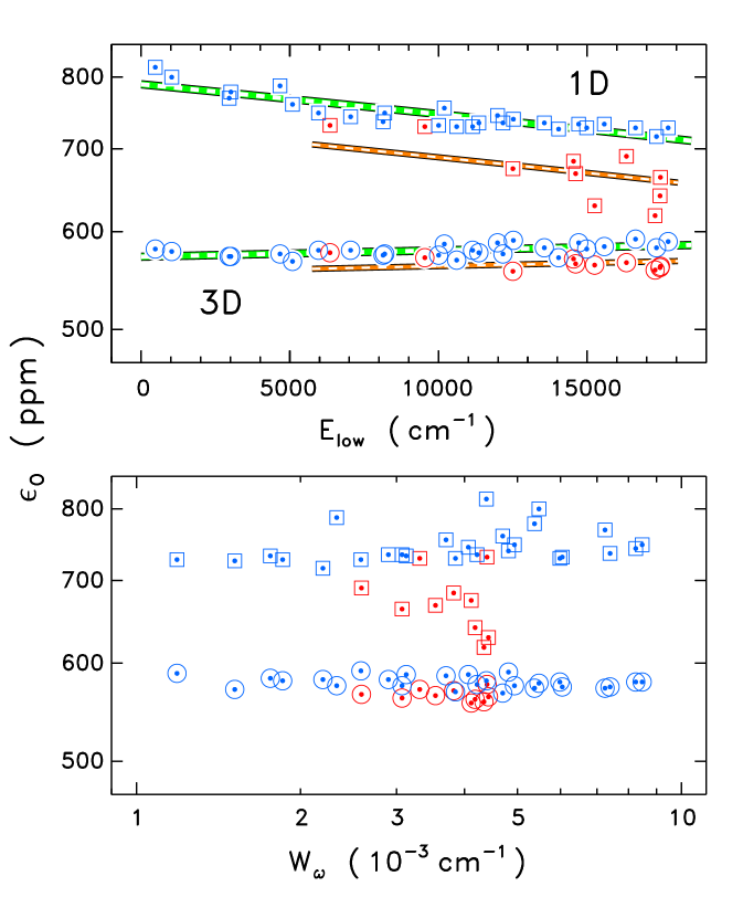
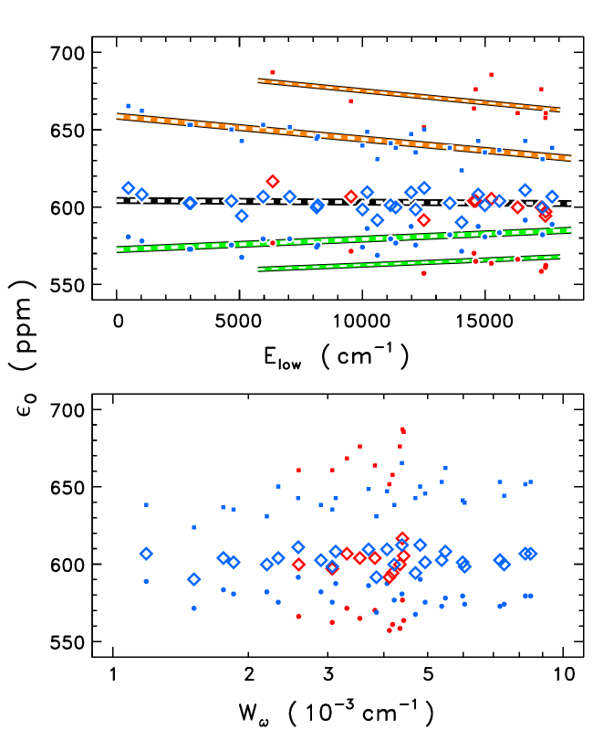
![[Uncaptioned image]](/html/1301.5281/assets/x16.png)
