Estimating norms of commutators

Abstract.

We discuss a general method of finding bounds on the norm of a commutator of an operator and a function of a normal operator. As an application we find new bounds on the norm of a commuator with a square root.

1. Norms of Commutators and functional calculus

For later versions of this paper please visit
https://repository.unm.edu/handle/1928/23462
UNM Lobo Vault 1928/23462

For $f$ a continuous function $\mathbb{R}$ that is periodic, period $2\pi$ always assumed, then we we will have need to apply if via functional calculus to both hermitian and unitary elements, in the latter case by interpreting $f$ as a function on the circle. Just to be clear, we introduce the notation

$$f[V]=\tilde{f}(V)$$

for $V$ any unitary element in a unital $C^{*}$-algebra $\mathcal{A}$, where

$$f(z)=f\left(-i\log(z)\right)$$

for any $z$ of modulus one. For example

$$\cos[V]=\tfrac{1}{2}V^{*}+\tfrac{1}{2}V.$$

It is trivial to prove that when an element $A$ in $\mathcal{A}$ commutes with $V$ then $A$ commutes with $f[V]$. We will need good estimates that quantify the statement that when $A$ almost commutes with $V$ then it also almost commutes with $f[V]$.

The only norm on $\left[A,V\right]$ we really care about is the operator norm, i.e. the norm on $\mathcal{A}$, that we denote $\left\|\cdot\right\|$. As to functions $f$ that are periodic, we need

$$\left\|f\right\|_{\infty}=\sup_{-\pi\leq x\leq\pi}\left|f(x)\right|$$

and, whenever $f$ has Fourier series converging absolutely, we use

$$\bigl{\|}f\bigr{\|}_{F}=\bigl{\|}\hat{f}\bigr{\|}_{1}$$

the $\ell^{1}$ norm of the Fourier series. We use $\mathcal{U}(A)$ for the group of unitaries in $\mathcal{A}$.

Definition 1.1.

Suppose $f$ is continous and periodic. Define $\eta_{f}:[0,\infty)\rightarrow[0,\infty)$ by

$$f_{\eta}(\delta)=\sup\left\{\left\|\left[f[V],A\right]\right\|\left|\,V\in\mathcal{U}(A),\left\|A\right\|\leq 1,\left\|\left[V,A\right]\right\|\leq\delta\right.\right\}$$

and the supremum is taken over every possible $C^{*}$-algebra $\mathcal{A}$ and taking $V$ and $A$ in $\mathcal{A}$.

There is a general trend where results about commutators are related to continuity results involving the functional calculus. See [1], for example. In the case of unitaries there is an easy connection between the two topics.

Lemma 1.2.

For $f$ that is continous and periodic, if $V$ and $V_{1}$ are unitaries then

$$\left\|f[V]-f[V_{1}]\right\|\leq\eta_{f}\left(\left\|V-V_{1}\right\|\right).$$

Proof.

Notice

$$\left\|\left[\left(\begin{array}[]{cc}0&1\\ 1&0\end{array}\right),\left(\begin{array}[]{cc}0&V\\ V_{1}&0\end{array}\right)\right]\right\|=\left\|V-V_{1}\right\|$$

and

$$\left\|\left[\left(\begin{array}[]{cc}0&1\\ 1&0\end{array}\right),\left(\begin{array}[]{cc}0&f[V]\\ f[V_{1}]&0\end{array}\right)\right]\right\|=\left\|f[V]-f[V_{1}]\right\|$$

so this is an easy calculation. ∎

The following generalizes a trick in Pedersen’s work on commutators and square roots, [4, Lemma 6.2].

Lemma 1.3.

Suppose $f$, $g$ and $h$ are continous and periodic, that $g^{\prime}$ has absolutely convergent Fourier series. If $f=g+h$ then

$$\eta_{f}(\delta)\leq m\delta+b$$

where

$$m=\left\|g^{\prime}\right\|_{F}$$

and

$$b=2\min_{\lambda\in\mathbb{C}}\left\|h-\lambda\right\|_{\infty}.$$

When $h$ is real valued then $b=\max(h)-\min(h)$.

Remark.

In the special case where $h=0$ we recover the folk theorem that says

(1.1) $$\left\|\left[g[V],A\right]\right\|\leq\left\|g^{\prime}\right\|_{F}\left\|\left[V,A\right]\right\|$$

for any unitary $V$ and any operator $A$, now without norm restriction because the two sides are homogeneous in $A$.

Proof.

Suppose $\left\|A\right\|\leq 1$ and $V$ is unitary. Since

$$\left\|\left[f[V],A\right]\right\|\leq\left\|\left[g[V],A\right]\right\|+\left\|\left[h[V],A\right]\right\|$$

and

$$\left\|\left[h[V],A\right]\right\|=\left\|\left[h[V]+\lambda I,A\right]\right\|=\left\|\left[\left(h+\lambda\right)[V],A\right]\right\|$$

it suffices to prove equation (1.1) and

(1.2) $$\left\|\left[h[V],A\right]\right\|\leq 2\left\|h\right\|_{\infty}.$$

We know

$$g(x)=\sum_{n=-\infty}^{\infty}a_{n}e^{inx}$$

where $\sum|na_{n}|<\infty$ and so

$$\left\|\left[g[V],A\right]\right\| =\left\|\left[\sum_{n=-\infty}^{\infty}a_{n}V^{n},A\right]\right\|$$

$$\leq\sum_{n=-\infty}^{\infty}\left|a_{n}\right|\left\|\left[V^{n},A\right]\right\|$$

$$\leq\sum_{n=-\infty}^{\infty}\left|na_{n}\right|\left\|\left[V,A\right]\right\|$$

$$=\left\|g^{\prime}\right\|_{F}\left\|\left[V,A\right]\right\|.$$

The spectral theorem tells us $\left\|h[V]\right\|\leq\left\|h\right\|_{\infty}$ and so

$$\left\|\left[h[V],A\right]\right\|=\left\|h[V]A-h[V]A\right\|\leq 2\left\|h[V]\right\|\left\|A\right\|\leq 2\left\|h\right\|_{\infty}.$$

∎

As an example, we attack the square root function $f(x)=\sqrt{x}$. However, this is for $0\leq H\leq 1$ replacing $V$ so is about $\gamma_{f}$ not $\eta_{f}$, where $\gamma_{f}$ we now define for working with functional calculus of postive contractions.

Definition 1.4.

Suppose $f$ is continous on $[0,1]$. Define $\eta_{f}:[0,\infty)\rightarrow[0,\infty)$ by

$$f_{\eta}(\delta)=\sup\left\{\left\|\left[f(H),A\right]\right\|\left|\,0\leq H\leq 1,\left\|A\right\|\leq 1,\left\|H\right\|\leq 1,\left\|\left[H,A\right]\right\|\leq\delta\right.\right\}$$

and the supremum is taken over every possible $C^{*}$-algebra $\mathcal{A}$ and taking $H$ and $A$ in $\mathcal{A}$.

Lemma 1.5.

Suppose $f$, $g$ and $h$ are continous on $[0,1]$ and that $g$ is analytic, with power series

$$g(x)=\sum_{n=0}^{\infty}a_{n}x^{n}.$$

If $f=g+h$ then

$$\eta_{f}(\delta)\leq m\delta+b$$

where

$$m=\sum_{n=0}^{\infty}\left|na_{n}\right|$$

and

$$b=2\min_{\lambda\in\mathbb{C}}\left\|h-\lambda\right\|_{\infty}.$$

Proof.

We know $\sum|na_{n}|<\infty$ and so

$$\left\|\left[g(H),A\right]\right\| =\left\|\left[\sum_{n=0}^{\infty}a_{n}H^{n},A\right]\right\|$$

$$=\left\|\sum_{n=0}^{\infty}a_{n}\left[H^{n},A\right]\right\|$$

$$\leq\sum_{n=0}^{\infty}\left|a_{n}\right|\left\|\left[H^{n},A\right]\right\|$$

$$\leq\sum_{n=0}^{\infty}\left|na_{n}\right|\left\|\left[H,A\right]\right\|.$$

It is not clear who first asseted the following, but it appears in [5]. ∎

Conjecture 1.6.

For $f(x)=\sqrt{x}$ we have $\gamma_{f}(\delta)=\sqrt{\delta}$. Equivalently

$$\left\|\left[H^{\frac{1}{2}},A\right]\right\|\leq\left\|\left[H,A\right]\right\|^{\frac{1}{2}}$$

wherever $0\leq H\leq 1$ and $\left\|A\right\|\leq 1$.

For any $a$ greater than $0$ and at most $1$ let $g$ be the Taylor expansion of $f$ at $a$,

$$g(x)=\frac{1}{2\sqrt{a}}(x-a)+\sqrt{a}.$$

and $h=f-g$,

$$h(x)=\sqrt{x}-\frac{1}{2\sqrt{a}}(x-a)-\sqrt{a}.$$

Clearly $\max(h)=h(a)=0$ and the minimum occurs at either $x=0$ or $x=1$, where the values are

$$h(0)=-\tfrac{1}{2}\sqrt{a}$$

and

$$h(1)=1-\frac{1}{2\sqrt{a}}-\frac{\sqrt{a}}{2}.$$

For $\tfrac{1}{4}\leq a\leq 1$ we find

$$\min(h)=-\tfrac{1}{2}\sqrt{a}.$$

Therefore,

(1.3) $$\eta_{f}(\delta)\leq\frac{1}{2\sqrt{a}}\delta+\tfrac{1}{2}\sqrt{a}$$

for $\tfrac{1}{4}\leq a\leq 1$, which is very interesting since at $\delta=a$ the right hand side is $\sqrt{a}$. We have proven a special case of the conjecture, which we state as a lemma.

Lemma 1.7.

When $0\leq H\leq 1$ and $\left\|A\right\|\leq 1$ and $\left\|\left[H,A\right]\right\|\geq\tfrac{1}{4}$, we have

$$\left\|\left[H^{\frac{1}{2}},A\right]\right\|\leq\left\|\left[H,A\right]\right\|^{\frac{1}{2}}.$$

Pedersen uses the following easy lemma.

Lemma 1.8.

If $f_{1}$ is continuous on $[0,1]$ and we set

$$f_{2}(x)=1-f_{1}(1-x)$$

that $\gamma_{f_{1}}=\gamma_{f_{2}}$.

His proof of the inequality

(1.4) $$\left\|\left[H^{\frac{1}{2}},A\right]\right\|\leq\frac{2}{\sqrt{\pi}}\left\|\left[H,A\right]\right\|^{\frac{1}{2}}$$

(notice $2\pi^{\frac{1}{2}}\approx 1.128$) in [4, Lemma 6.2] invokes Lemma 1.5 infinitely many times, as $g$ ranges over the Taylor polynomials for $f(x)=1-\sqrt{1-x}$ exanded at $0$. While (1.4) is the statement

$$\gamma_{f}(\delta)\leq\frac{2}{\sqrt{\pi}}\delta^{\frac{1}{2}}$$

what he actually proves is a bound that is significantly smaller for $\delta$ close to $1$. Indeed, he showed $\gamma_{f}$ to be bounded by the function shown in Figure 1.1

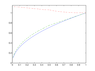
Figure 1.1. Bound on $\left\|\left[H^{\frac{1}{2}},A\right]\right\|$ for varying values of $\left\|\left[H,A\right]\right\|$ as found by Pedersen, shown as a dashed line. The solid curve is $\sqrt{\delta}$. The top curve is the ratio of the bound to $\sqrt{\delta}$.

The mininum of all these lines does not lead to an easy formula, so we state our best theorem regarding the square root in terms on a ploted function.

Theorem 1.9.

If $0\leq H\leq 1$ and $\left\|A\right\|\leq 1$ then

$$\left\|\left[H^{\frac{1}{2}},A\right]\right\|\leq\gamma_{0}\left(\left\|\left[H,A\right]\right\|\right)$$

where $\gamma$ is the function illustrated in Figure 1.2.

Proof.

We simply combine all the linear bounds in [4, Lemma 6.2] with Lemma 1.7. ∎

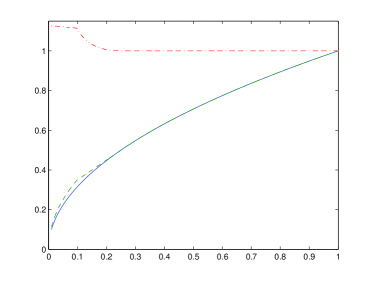
Figure 1.2. Bound on $\left\|\left[H^{\frac{1}{2}},A\right]\right\|$ for varying values of $\delta=\left\|\left[H,A\right]\right\|$ as improved by the inequalities (1.3). The solid curve is $\sqrt{\delta}$. The dashed curve is the upper bound $\gamma_{0}(\delta)$ of Thereom 1.9. The top curve is $\gamma_{0}(\delta)/\sqrt{\delta}$.

2. Examples involving functions on the circle

There is a desire, driven by investigations in physics [3], to get quantitative results regarding almost commuting matrices. The Bott index for almost commuting matrices depends on the functional calculus of unitary matrices. Quantitative studies of the Bott index require triples of functions

$$f,g,h:\mathbb{T}^{2}\rightarrow\mathbb{R}^{3}$$

with certain topological properies. Having a method for dealing with $\left\|\left[f[V],U\right]\right\|$for a pair of unitary elements was the primary motivation for the present paper.

Corollary 2.1.

If $f$ has uniformly converent Fourier series,

$$f(x)=\sum_{n=-\infty}^{\infty}a_{n}e^{inx}$$

then

$$\eta_{f}(\delta)\leq 2\sum_{n=-\infty}^{\infty}|a_{n}|.$$

and

(2.1) $$\eta_{f}(\delta)\leq\delta\sum_{n=-N}^{N}|na_{n}|+2\sum_{n=N+1}^{\infty}\left(|a_{n}|+|a_{-n}|\right).$$

Proof.

If we take set

$$g(x)=\sum_{n=-N}^{N}a_{n}e^{inx}$$

and apply Lemma 1.3 we obtain (2.1). For the other we set $g$ to $0$. ∎

Example 2.2.

Consider the triangle wave

$$f(x)=\begin{cases}1+\frac{2}{\pi}x&-\pi\leq x\leq 0\\ 1-\frac{2}{\pi}x&0\leq x\leq\pi\end{cases}$$

we have $a_{2n}=0$ and

$$a_{2n-1}=\frac{8}{\pi^{2}}\frac{1}{(2n-1)^{2}}.$$

Using Corollary 2.1 we get the bound on $\eta_{f}$ as indicated in Figure 2.1. Slighlty better estimates are possible if we exactly compute the min and max of the difference between $f$ and its triginometric polynomial approximations. We could also eliminate the corners by interpolating with trig polynomials between the truncated Fourier series.

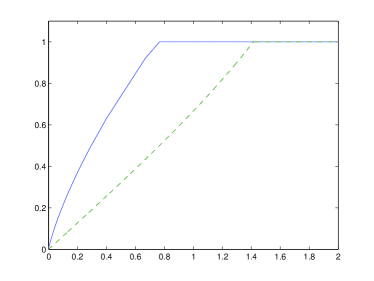
Figure 2.1. Bounds on $\left\|\left[f[V],A\right]\right\|$ for varying values of $\delta=\left\|\left[V,A\right]\right\|$ for $f$ a triangle wave. The solid line is an upper bound and the dashed line is a lower bound.

The triangle wave is, up to scaling, the function used in [2] as one of the functions defining the Bott invariant. To see how well we are doing in bounding $\left\|\left[f[V],A\right]\right\|$ we consider a crude lower bound.

Lemma 2.3.

If $f$ is periodic and continuous then for any $\delta<2$ we have

$$\eta_{f}(\delta)\geq\max\left\{\left|f(x_{2})-f(x_{1})\right|\,\left|\,\left|x_{2}-x_{1}\right|\leq 2\arcsin\left(\tfrac{\delta}{2}\right)\right.\right\}.$$

The follows easily from examining the commutator of

$$\left(\begin{array}[]{cc}0&1\\ 1&0\end{array}\right)$$

with

$$\left(\begin{array}[]{cc}e^{ix_{2}}&0\\ 0&e^{ix_{2}}\end{array}\right)$$

and

$$f\left[\left(\begin{array}[]{cc}e^{ix_{2}}&0\\ 0&e^{ix_{2}}\end{array}\right)\right]=\left(\begin{array}[]{cc}f(x_{1})&0\\ 0&f(x_{2})\end{array}\right).$$

Thus in the example of the triangle wave, we could may have considerable room to improve our estimate. However, for the purposes of “quantitative $K$-theory” involving the Bott index, this $f$ shows limited potential, as its companion functions $g$ and $h$ are not so nice. That is, in the Bott index definition as in [2] we also need

(2.2) $$h(x)=\begin{cases}\sqrt{1-\frac{4}{\pi^{2}}x^{2}}&\mbox{ if }x\in\left[-\frac{\pi}{2},\frac{\pi}{2}\right]\\ 0&\mbox{ if }x\notin\left[-\frac{\pi}{2},\frac{\pi}{2}\right]\end{cases}$$

and $\eta_{h}$ tends to zero rather slowly. The crude lower bound from Lemma 2.3 is shown in Figure 2.2. This is one reason for the switch to a different triple of functions $f$, $g$ and $h$ in [3]. Commutators involving the functions in the new and improved Bott index will be analyized elsewhere.

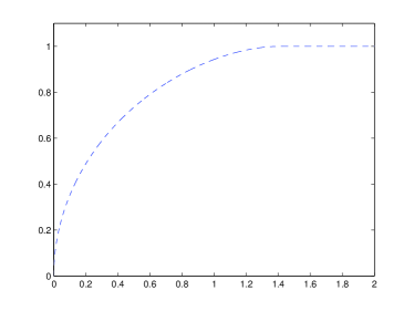
Figure 2.2. A lower bound on $\left\|\left[h[V],A\right]\right\|$ where $h$ is the bump function on the circle defined in Equation 2.2.

3. Acknowledgements

This work was partially supported by a grant from the Simons Foundation (208723 to Loring).

References

[1]R. Bhatia and F. Kittaneh, Some inequalities for norms of
commutators, SIAM J. Matrix Anal. Appl., 18 (1997), pp. 258–263.
[2]R. Exel and T. A. Loring, Invariants of almost commuting unitaries,
J. Funct. Anal., 95 (1991), pp. 364–376.
[3]M. B. Hastings and T. A. Loring, Topological insulators and -algebras: Theory and numerical practice, Ann. Physics, 326 (2011),
pp. 1699–1759.
[4]G. K. Pedersen, The corona construction, in Operator Theory:
Proceedings of the 1988 GPOTS-Wabash Conference (Indianapolis,
IN, 1988), vol. 225 of Pitman Res. Notes Math. Ser., Longman Sci. Tech.,
Harlow, 1990, pp. 49–92.
[5], A commutator
inequality, in Operator algebras, mathematical physics, and low-dimensional
topology (Istanbul, 1991), vol. 5 of Res. Notes Math., A K Peters,
Wellesley, MA, 1993, pp. 233–235.