Phase transition in a coevolving network of conformist and contrarian voters

Abstract

In the coevolving voter model, each voter has one of two diametrically opposite opinions, and a voter encountering a neighbor with the opposite opinion may either adopt it or rewire the connection to another randomly chosen voter sharing the same opinion. As we smoothly change the relative frequency of rewiring compared to that of adoption, there occurs a phase transition between an active phase and a frozen phase. By performing extensive Monte Carlo calculations, we show that the phase transition is characterized by critical exponents $\beta=0.54(1)$ and $\bar{\nu}=1.5(1)$, which differ from the existing mean-field-typed prediction. We furthermore extend the model by introducing a contrarian type that tries to have neighbors with the opposite opinion, and show that the critical behavior still belongs to the same universality class irrespective of such contrarians’ fraction.

I INTRODUCTION

Analyzing social dynamics from a physical viewpoint has become an important topic in statistical physics. In particular, emergence of collective opinion is an intriguing phenomenon which can be readily compared to the collective ordering manifested in many statistical-physical systems, and the voter model has served as an insightful starting point to study the opinion dynamics *[See; e.g.; ][forfurtherreferences.]CastellanoRMP. When the voter model began to be investigated in the context of complex networks, the underlying connection structure among voters was usually assumed to be static. In this case, the dynamics can be basically described as follows: The opinion $S_{j}$ assigned to a voter $j$ is either $+1$ or $-1$ like an Ising spin. For a given voter $j$, we randomly choose one of the neighbors, say $k$. If $S_{j}\neq S_{k}$, the link between $j$ and $k$ is called active, and $j$ adopts $k$’s opinion under certain stochastic rules. As implied in this adoption mechanism, it is true that our opinion is shaped by whom we are surrounded by, but it can be equally true that our opinion shapes our social networks. So the situation becomes more interesting when we allow voters to change their neighbors. It then looks natural to introduce a tendency to connect to like-minded people, because as the proverb says, birds of a feather flock together. This simultaneous change in the network structure is termed coevolution, and the voter model has been studied in this coevolutionary framework for the natural reason mentioned above Vazquez et al. (2008); Durrett et al. (2012); *BenczikPRE; *FuPRE; Holme and Newman (2006); Iñiguez et al. (2011). Besides the opinion dynamics, we can also mention that the coevolutionary dynamics plays a crucial role in the context of epidemiology since adaptation of a network structure in response to disease spreading is directly related to quarantine policies (see Refs. Gross et al. (2006); *GrossROYAL; *CrokIOP; Shaw and Schwartz (2008) for theoretical investigations). In addition, more physically motivated studies include a coevolving network of phase oscillators Aoki and Aoyagi (2009), the kinetic Ising model with Glauber-like dynamics Mandrà et al. (2009); *HajraEPJB, and a variation of the $XY$ model Holme et al. (2009).

II COEVOLVING NETWORK OF VOTERS

In this work, we begin with the coevolving voter model proposed by Vazquez et al. Vazquez et al. (2008) where an active link becomes inert either by rewiring with probability $p$ or by adoption with probability $1-p$ (see also Ref. Cheng et al. (2010); *HerreraEPL; *NardiniPRL; *ZschalerPRE for its extended versions). According to a mean-field (MF) argument and numerical simulations, this model has a well-defined phase transition at a critical value $p_{c}$, separating an active phase from a frozen phase in which one observes no active links between the two different opinions. Specifically, as $p$ approaches the critical point $p_{c}$ from below, the active-link density is expected to scale as $\rho\sim(p_{c}-p)^{\beta}$, or equivalently, $\rho\sim N^{-\beta/\bar{\nu}}$ at $p=p_{c}$ for a large but finite number $N$ of voters, where $\beta$ and $\bar{\nu}$ are critical indices. The MF argument in Ref. Vazquez et al. (2008) predicts $\beta=1$ and $p_{c}=(\mu-2)/(\mu-1)$, where $\mu$ means the average degree. Although this predicted $p_{c}$ significantly deviates from numerical estimates, there are better methods to estimate $p_{c}$ Böhme and Gross (2011). However, it has not been questioned whether the critical behavior is consistent with the MF prediction, and we will show that this is not the case by finding $\beta=0.54(1)$ and $\bar{\nu}=1.5(1)$. Then, we extend the model by introducing a peculiar voter type that tries to surround herself with the opposite opinion, which might be called heterophily Kimura and Hayakawa (2008). The effect of such behavior has already been studied in opinion dynamics Galam (2004); Crokidakis and Anteneodo (2012); *BiswasAX and Ref. De La Lama et al. (2007) has argued that such behavior can be generated by stochasticity. Though this heterophilic dynamics is sometimes dubbed the “inverse voter” model Zhu et al. (2011), let us denote the usual voter and the inverse voter as a conformist ($v$) and a contrarian (${\bar{v}}$), respectively, following the terminology in Refs. Galam (2004); Hong and Strogatz (2011). Our point is that the critical behavior is universal regardless of such contrarians’ fraction whereas $p_{c}$ is a nonuniversal quantity.

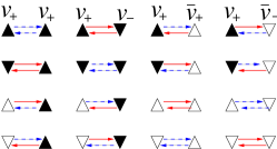
Figure 1: (Color online) Possible states of a link between a pair of voters. We represent a conformist as a filled triangle, pointing up ($\blacktriangle$) or down ($\blacktriangledown$) depending on the opinion. Likewise, a contrarian is represented as an empty triangle ($\vartriangle$ or $\triangledown$). A full red arrow and a dashed blue arrow mean an active link and an inert one, respectively. Whether a link is active depends on whose viewpoint is taken, so an arrow from a voter means the state of the link from her viewpoint. For example, the link between $\triangledown$ and $\blacktriangle$ is active from $\blacktriangle$’s viewpoint, while it is inert from $\triangledown$’s viewpoint (bottom left).

For simplicity, we assume that voters do not change their types, (i.e., once a contrarian, forever a contrarian) so the fraction $r$ of conformists is constant in time. When $r=1$, our model is reduced to the original one in Ref. Vazquez et al. (2008), while for $r=0$, it is identical to the inverse voter model in Ref. Zhu et al. (2011). It is important to note that whether a link is active between two voters depends on their types: Fig. 1 shows all the possible link configurations between two voters, where the signs mean their opinions. Although each link is expressed as two directed arrows, there exists only one single link between a pair of voters so the double arrows imply that the state of a link is not uniquely defined, in general. For example, if a conformist with opinion $+1$ is linked to a contrarian with $-1$, the conformist regards the link as active while the contrarian regards it as inert. If a link connecting two voters is regarded by both as active (inert), the link contributes $1$ ($0$) to the total number of active links in the system. If only one of them regards it as active, on the other hand, it is counted as one-half.

Let us now explain details of our calculation. In terms of a network, a voter is mapped to a node, and a link connecting nodes $j$ and $k$ can be denoted as $(j,k)$. As an initial condition, we construct a regular random network of size $N$ where every node has exactly $\mu$ neighbors (we choose $\mu=4$ throughout this work). We then randomly select $rN$ nodes as conformists while the others are set to be contrarians. Every node has equally random probability to have either opinion at the starting point. Then, we randomly pick up a node $j$ and choose one of its neighbors, say $k$, also at random. If the link $(j,k)$ is inert from $j$’s viewpoint, nothing happens. If it is not, there are two possible options: With probability $p$, $(j,k)$ is rewired to a randomly chosen node $l$ in such a way that $(j,l)$ becomes inert from $j$’s viewpoint. Or with probability $1-p$, $S_{j}$ is flipped to make $(j,k)$ inert from $j$’s viewpoint. At each time step $t$, this updating procedure is repeated for $N$ times.

III RESULTS

We take the active-link density $\rho$ as an order parameter whose dependence on $N$ at $p=p_{c}$ provides estimates of the critical indices. In order to find its stationary value for each $N$, $\rho$ should be first measured as a function of $t$ over $N_{s}$ independent samples. Note that we measure surviving average by including only samples with at least one active link at each given time $t$. This surviving-averaged quantity shows transient behavior at small $t$, whereas it fluctuates violently at large $t$ as statistics become poor with few surviving samples. So the stationary value $\rho(N)$ is estimated by taking an average over a certain time interval $[t_{1},t_{2}]$. In our case, the lower bound $t_{1}$ is chosen as $5\times 10^{2}$ or $10^{3}$ depending on $N$, while $t_{2}$ is fixed at $5\times 10^{3}$. The error bar becomes generally smaller as $N_{s}$ increases, and we find it quite enough to work with $N_{s}=10^{4}$ for $r=1/2$ and $N_{s}=2\times 10^{5}$ for $r=0$ or $r=1$. In addition, as for the system size $N$, we need to consider two limitations: That is, if $N$ is too small, it is difficult to generate many surviving samples at large $t$ since $\rho=0$ is an absorbing state which can always be reached due to fluctuations in a finite-sized system. If $N$ is too large, on the other hand, it is difficult to approach a stationary value, especially near the critical point, due to the diverging relaxation time scale. For these reasons, we will concentrate on precise estimates of $\rho(N)$ from $N=10^{3}$ to $N=2\times 10^{3}$.

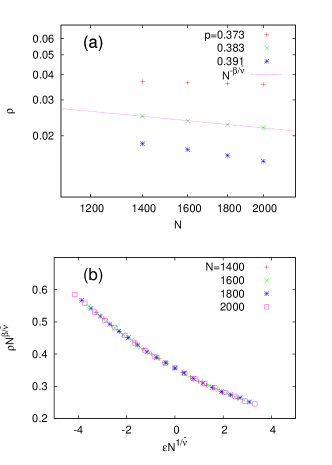
Figure 2: (Color online) Coevolving voter model with $r=1$ where all voters are conformists. (a) The stationary active-link density $\rho$ is plotted as a function of $N$ at different rewiring probabilities. The solid line is a guide to eyes. (b) The function $f$ in Eq. (1) is obtained by scaling collapse with $\bar{\nu}=1.5(1)$, $\beta=0.54(1)$, and $p_{c}=0.383(1)$.

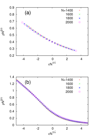
Figure 3: (Color online) (a) Scaling collapse for $r=0$ where all voters are contrarians and (b) for $r=1/2$. The critical exponents $\beta/\bar{\nu}=0.37(2)$ and $\bar{\nu}=1.5(1)$ are used in common, whereas $p_{c}=0.383(1)$ in panel (a) in contrast to $p_{c}=0.790(1)$ in panel (b).

We start with $r=1$ and plot numerical results of $\rho(N)$ at various values of $p$ in Fig. 2(a). It is observed that $\rho$ decays algebraically at $p\approx 0.383$, indicating the existence of a continuous phase transition at $p_{c}=0.383(1)$, in agreement with $p_{c}\approx 0.38$ found by numerical simulations in Ref. Vazquez et al. (2008). From the standard finite-size scaling form

$$\rho=N^{-\beta/\bar{\nu}}f(\varepsilon N^{1/\bar{\nu}})$$ (1)

with $\varepsilon\equiv(p-p_{c})/p_{c}$, the slope of the line in Fig. 2(a) determines $\beta/\bar{\nu}\approx 0.36$. We use these values of $p_{c}$ and $\beta/\bar{\nu}$ to make the data collapse in Fig. 2(b). This analysis finds that $p_{c}=0.383(1)$, $\bar{\nu}=1.5(1)$, and $\beta=0.54(1)$. It is noteworthy that the actual value of $\beta$ is far from the MF prediction that $\beta=1$. The reason is that the full mixing assumption of the MF approach cannot be justified when the system splits into clusters, which is exactly what happens at the critical point [see Fig. 5(a) below]. In this respect, it should not be surprising that the actual transition is not of the MF type.

We then repeat the same analysis for $r=0$ [Fig. 3(a)]. The resulting exponents $\beta/\bar{\nu}=0.37(2)$ and $\bar{\nu}=1.5(1)$ as well as $p_{c}=0.383(1)$ are in striking agreement with those in the above case with $r=1$. From the observation that both with $r=0$ and $r=1$ belong to the same universality class characterized by the same critical exponents $\beta$ and $\bar{\nu}$, one might guess that this holds true for any value of $r\in[0,1]$. In order to check this, one could perform the same finite-size scaling analysis for $r=1/2$ [Fig. 3(b)]. Unfortunately, finite-size corrections to scaling are so substantial in our data that we should be content with a consistency check just by tuning $p_{c}$ with having fixed $\beta/\bar{\nu}=0.37$ and $\bar{\nu}=1.5$. In spite of such limitations, we can say that the result is not inconsistent with the guess. It is somewhat interesting to note that the coevolving model in Ref. Holme and Newman (2006) has $1/\bar{\nu}\approx 0.7(1)$, which is also close to our finding $1/\bar{\nu}\approx 0.67$.

Figure 4: Phase diagram of the model on the $(p,r)$ plane. See text for details.

Let us now turn our attention to determining the critical threshold to find the shape of the phase boundary. The estimate of $p_{c}$ in the simple MF approximation by Vazquez et al. Vazquez et al. (2008) can be briefly explained in the following way: Suppose that there is one active link in the system with average degree $\mu$. For example, there are two clusters of opposite opinions and there is one single link between them. If the link is rewired with probability $p$, this active link will disappear. If one voter changes the opinion with probability $1-p$, then the original active link disappears but all the other $\mu-1$ links become active. Therefore, the expected change in the number of active links is $[(\mu-1)-1](1-p)-p$, which is zero below the threshold, leading to $p_{c}=(\mu-2)/(\mu-1)$. Note that the above simple MF approximation does not depend on the value of $r$, and thus giving $p_{c}=2/3$ for $\mu=4$ irrespective of $r$, which is sharply against our observation that $p_{c}(r=1/2)\neq p_{c}(r=1)$.

In order to numerically obtain the actual phase diagram on the $(p,r)$ plane, we first measure $\rho^{\ast}\equiv\rho(p=p_{c}=0.383)$ at $r=1$ for size $N=10^{3}$ and then use the same $\rho^{\ast}$ to locate $p_{c}$ for other values of $r$. In other words, $p_{c}(r)$ is roughly estimated from the condition that $\rho(p_{c};r,N=10^{3})=\rho^{\ast}$. We have confirmed that this simple method yields $p_{c}$ reasonably close to the the above-mentioned estimates for $r=0$ and $r=1/2$. Furthermore, it is enough to use a smaller ensemble ($N_{s}=200$) for the present purpose. The resulting phase diagram shows a lobelike shape with a maximum value around $r=1/2$ (Fig. 4), and the MF theory fails to predict this feature once again.

In order to understand such a shape, let us look into the MF estimate a little further: In updating a node with the probability $1-p$, it is possible to come back to the original configuration by flipping the same node once again. This possibility is ignored in the simple MF scheme in Ref. Vazquez et al. (2008), which means that the spatial correlation among the newly created active links is ignored. The $q$-fan motif method Böhme and Gross (2011) is a more advanced approximation in the sense that it evolves the configuration until clusters of the active links are separated by at least one spacing. If the configuration is expressed with a finite number of separate clusters of active links after some time, then the method ignores the spatial correlation among them in describing their further evolution with a stochastic matrix. Comparing $r=0$ with $r=1$, we see that the $q$-fan motif method works in the same way and the resulting estimates of $p_{c}$ are therefore identical again. When $0<r<1$, however, there arises an important difference that there can exist an active link between a conformist and a contrarian, which never disappears just by changing one’s opinion. There is always a finite chance that a cluster of active links keeps growing from this active seed link by flipping neighboring voters. Thus the configuration cannot be generally a collection of finite separated clusters for $0<r<1$, and the $q$-fan motif method fails in estimating $p_{c}$. Nevertheless, it tells us that one needs a higher $p$ in order to suppress such growth of the cluster by rewiring the active link instead of changing opinions. This qualitatively explains why the phase boundary at $0<r<1$ is pushed to higher $p$ in Fig. 4.

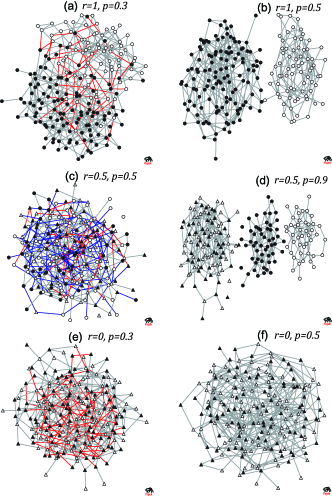
Figure 5: (Color online) Snapshots of network structures in the active phase [(a), (c), (e)] and in the frozen phase [(b), (d), (f)] with $r=1$ [(a),(b)], $r=1/2$ [(c),(d)], and $r=0$ [(e),(f)]. The number of nodes is $N=200$ in each case. Circles and triangles denote conformists and contrarians, respectively, and a filled (empty) symbol denotes the opinion $+1$ ($-1$). Red, blue, and gray colors mean that the link is active in both directions, active in only one direction, and inert in both directions, respectively. All links become inert (gray) in the frozen phase.

Finally, we visualize actual network structures in Fig. 5. When everyone is a conformist ($r=1$), one can clearly see that the network structure radically changes as $p$ passes the critical point so that the frozen phase is characterized by completely segregated opinions. More specifically, as $p_{c}$ is approached from below, two clusters have fewer and fewer inter-cluster links and they get disconnected at $p_{c}$. Therefore, in the vicinity of the critical point, the full-mixing assumption in the simple MF approximation just breaks down, allowing the critical exponents to deviate from the MF ones, as confirmed in the present work. We add a remark that network structures in the frozen phase largely depend on the conformist fraction $r$. For example, when $r=1/2$, the system usually splits into three clusters, one for contrarians and the other two for conformists.

IV SUMMARY

In summary, we have numerically studied the phase transition of the coevolving voter model composed of conformists and contrarians. Our main result suggests that the simple MF approximation cannot explain the transition nature, and that the universality class is well characterized by critical exponents $\beta\approx 0.54$ and $\nu\approx 1.5$, irrespective of the conformist fraction. We present the full phase diagram on the $(p,r)$ plane, which shows a symmetric lobelike structure around $r=1/2$.