Dynamic Functional Principal Components

Abstract

Abstract. In this paper, we address the problem of dimension reduction for time series of functional data $(X_{t}\colon t\in\mathbb{Z})$. Such functional time series frequently arise, e.g., when a continuous-time process is segmented into some smaller natural units, such as days. Then each $X_{t}$ represents one intraday curve. We argue that functional principal component analysis (FPCA), though a key technique in the field and a benchmark for any competitor, does not provide an adequate dimension reduction in a time-series setting. FPCA indeed is a static procedure which ignores the essential information provided by the serial dependence structure of the functional data under study. Therefore, inspired by Brillinger’s theory of dynamic principal components, we propose a dynamic version of FPCA, which is based on a frequency-domain approach. By means of a simulation study and an empirical illustration, we show the considerable improvement the dynamic approach entails when compared to the usual static procedure.

¹ Department of Mathematics, Université libre de Bruxelles (ULB), CP210, Bd. du Triomphe, B-1050 Brussels, Belgium.

² ECARES, Université libre de Bruxelles (ULB), CP 114/04 50, avenue F.D. Roosevelt B-1050 Brussels, Belgium.

³ ORFE, Princeton University, Sherrerd Hall, Princeton, NJ 08540, USA.

Keywords. Dimension reduction, frequency domain analysis, functional data analysis, functional time series, functional spectral analysis, principal components, Karhunen-Loève expansion.

1 Introduction

The tremendous technical improvements in data collection and storage allow to get an increasingly complete picture of many common phenomena. In principle, most processes in real life are continuous in time and, with improved data acquisition techniques, they can be recorded at arbitrarily high frequency. To benefit from increasing information, we need appropriate statistical tools that can help extracting the most important characteristics of some possibly high-dimensional specifications. Functional data analysis (FDA), in recent years, has proven to be an appropriate tool in many such cases and has consequently evolved into a very important field of research in the statistical community.

Typically, functional data are considered as realizations of (smooth) random curves. Then every observation $X$ is a curve $(X(u)\colon u\in\mathcal{U})$. One generally assumes, for simplicity, that $\mathcal{U}=[0,1]$, but $\mathcal{U}$ could be a more complex domain like a cube or the surface of a sphere. Since observations are functions, we are dealing with high-dimensional – in fact intrinsically infinite-dimensional – objects. So, not surprisingly, there is a demand for efficient data-reduction techniques. As such, functional principal component analysis (FPCA) has taken a leading role in FDA, and functional principal components (FPC) arguably can be seen as the key technique in the field.

In analogy to classical multivariate PCA (see Jolliffe [22]), functional PCA relies on an eigendecomposition of the underlying covariance function. The mathematical foundations for this have been laid several decades ago in the pioneering papers by Karhunen [23] and Loève [26], but it took a while until the method was popularized in the statistical community. Some earlier contributions are Besse and Ramsay [5], Ramsay and Dalzell [30] and, later, the influential books by Ramsay and Silverman [31], [32] and Ferraty and Vieu [11]. Statisticians have been working on problems related to estimation and inference (Kneip and Utikal [24], Benko et al. [3]), asymptotics (Dauxois et al. [10] and Hall and Hosseini-Nasab [15]), smoothing techniques (Silverman [34]), sparse data (James et al. [21], Hall et al. [16]), and robustness issues (Locantore et al. [25], Gervini [12]), to name just a few. Important applications include FPC-based estimation of functional linear models (Cardot et al. [9], Reiss and Ogden [33]) or forecasting (Hyndman and Ullah [20], Aue et al. [1]). The usefulness of functional PCA has also been recognized in other scientific disciplines, like chemical engineering (Gokulakrishnan et al. [14]) or functional magnetic resonance imaging (Aston and Kirch [2], Viviani et al. [37]). Many more references can be found in the above cited papers and in Sections 8–10 of Ramsay and Silverman [32], where we refer to for background reading.

Most existing concepts and methods in FDA, even though they may tolerate some amount of serial dependence, have been developed for independent observations. This is a serious weakness, as in numerous applications the functional data under study are obviously dependent, either in time or in space. Examples include daily curves of financial transactions, daily patterns of geophysical and environmental data, annual temperatures measured on the surface of the earth, etc. In such cases, we should view the data as the realization of a functional time series $(X_{t}(u)\colon t\in\mathbb{Z})$, where the time parameter $t$ is discrete and the parameter $u$ is continuous. For example, in case of daily observations, the curve $X_{t}(u)$ may be viewed as the observation on day $t$ with intraday time parameter $u$. A key reference on functional time series techniques is Bosq [8], who studied functional versions of AR processes. We also refer to Hörmann and Kokoszka [19] for a survey.

Ignoring serial dependence in this time-series context may result in misleading conclusions and inefficient procedures. Hörmann and Kokoszka [18] investigate the robustness properties of some classical FDA methods in the presence of serial dependence. Among others, they show that usual FPCs still can be consistently estimated within a quite general dependence framework. Then the basic problem, however, is not about consistently estimating traditional FPCs: the problem is that, in a time-series context, traditional FPCs are not the adequate concept of dimension reduction anymore – a fact which, since the seminal work of Brillinger [6], is well recognized in the usual vector time-series setting. FPCA indeed operates in a static way: when applied to serially dependent curves, it fails to take into account the potentially very valuable information carried by the past values of the functional observations under study. In particular, a static FPC with small eigenvalue, hence negligible instantaneous impact on $X_{t}$, may have a major impact on $X_{t+1}$, and high predictive value.

Besides their failure to produce optimal dimension reduction, static FPCs, while cross-sectionally uncorrelated at fixed time $t$, typically still exhibit lagged cross-correlations. Therefore the resulting FPC scores cannot be analyzed componentwise as in the i.i.d. case, but need to be considered as vector time series which are less easy to handle and interpret.

These major shortcomings are motivating the present development of dynamic functional principal components (dynamic FPCs). The idea is to transform the functional time series into a vector time series (of low dimension, $\leq 4$, say), where the individual component processes are mutually uncorrelated (at all leads and lags; autocorrelation is allowed, though), and account for most of the dynamics and variability of the original process. The analysis of the functional time series can then be performed on those dynamic FPCs; thanks to their mutual orthogonality, dynamic FPCs moreover can be analyzed componentwise. In analogy to static FPCA, the curves can be optimally reconstructed/approximated from the low-dimensional dynamic FPCs via a dynamic version of the celebrated Karhunen-Loève expansion.

Dynamic principal components first have been suggested by Brillinger [6] for vector time series. The purpose of this article is to develop and study a similar approach in a functional setup. The methodology relies on a frequency-domain analysis for functional data, a topic which is still in its infancy (see, for instance, Panaretos and Tavakoli 2013a).

The rest of the paper is organized as follows. In Section 2 we give a first illustration of the procedure and sketch two typical applications. In Section 3, we describe our approach and state a number of relevant propositions. We also provide some asymptotic features. In Section 4, we discuss its computational implementation. After an illustration of the methodology by a real data example on pollution curves in Section 5, we evaluate our approach in a simulation study (Section 6). Appendices A and B detail the mathematical framework and contain the proofs. Some of the more technical results and proofs are outsourced to Appendix C.

After the present paper (which has been available on Arxiv since October 2012) was submitted, another paper by Panaretos and Tavakoli (2013b) was published, where similar ideas are proposed. While both papers aim at the same objective of a functional extension of Brillinger’s concept, there are essential differences between the solutions developed. The main result in Panaretos and Tavakoli (2013b) is the existence of a functional process $(X_{t}^{*})$ of rank $q$ which serves as an “optimal approximation” to the process $(X_{t})$ under study. The construction of $(X_{t}^{*})$, which is mathematically quite elegant, is based on stochastic integration with respect to some orthogonal-increment (functional) stochastic process $(Z_{\omega})$. The disadvantage, from a statistical perspective, is that this construction is not explicit, and that no finite-sample version of the concept is provided – only the limiting behavior of the empirical spectral density operator and its eigenfunctions is obtained. Quite on the contrary, our Theorem 3 establishes the consistency of an empirical, explicitly constructed and easily implementable version of the dynamic scores – which is what a statistician will be interested in. We also remark that we are working under milder technical conditions.

2 Illustration of the method

An impression of how well the proposed method works can be obtained from Figure 1. Its left panel shows ten consecutive intraday curves of some pollutant level (a detailed description of the underlying data is given in Section 5). The two panels to the right show one-dimensional reconstructions of these curves. We used static FPCA in the central panel and dynamic FPCA in the right panel.

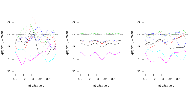
Figure 1: Ten successive daily observations (left panel), the corresponding static Karhunen-Loève expansion based on one (static) principal component (middle panel), and the dynamic Karhunen-Loève expansion with one dynamic component (right panel). Colors provide the matching between the actual observations and their Karhunen-Loève approximations.

The difference is notable. The static method merely provides an average level, exhibiting a completely spurious and highly misleading intraday symmetry. In addition to daily average levels, the dynamic approximation, to a large extent, also catches the intraday evolution of the curves. In particular, it retrieves the intraday trend of pollution levels, and the location of their daily spikes and troughs (which varies considerably from one curve to the other). For this illustrative example we chose one-dimensional reconstructions, based on one single FPC; needless to say, increasing the number of FPCs (several principal components), we obtain much better approximations – see Section 4 for details.

Applications of dynamic PCA in a time series analysis are the same as those of static PCA in the context of independent (or uncorrelated) observations. This is why obtaining mutually orthogonal principal components – in the sense of mutually orthogonal processes – is a major issue here. This orthogonality, at all leads and lags, of dynamic principal components, indeed, implies that any second-order based method (which is the most common approach in time series) can be carried out componentwise, i.e.  via scalar methods. In contrast, static principal components still have to be treated as a multivariate time series.

Let us illustrate this superiority of mutually orthogonal dynamic components over the auto- and cross-correlated static ones by means of two examples.

Change point analysis: Suppose that we wish to find a structural break (change point) in a sequence of functional observations $X_{1},\ldots,X_{n}$. For example, Berkes et al. [4] consider the problem of detecting a change in the mean function of a sequence of independent functional data. They propose to first project data on the $p$ leading principal components and argue that a change in the mean will show in the score vectors, provided hat the proportion of variance they are accounting for is large enough. Then a CUSUM procedure is utilized. The test statistic is based on the functional

$$T_{n}(x)=\frac{1}{n}\sum_{m=1}^{p}\hat{\lambda}_{m}^{-1}\left(\sum_{1\leq k\leq nx}\hat{Y}^{\text{stat}}_{mk}-x\sum_{1\leq k\leq n}\hat{Y}^{\text{stat}}_{mk}\right)^{2},\quad 0\leq x\leq 1.$$

Here $\hat{Y}^{\text{stat}}_{mk}$ is the $m$-th empirical PC score of $X_{k}$ and $\hat{\lambda}_{m}$ is the $m$-th largest eigenvalue of the empirical covariance operator related to the functional sample. The assumption of independence implies that $T_{n}(x)$ converges, under the no-change hypothesis, to the sum of $p$ squared independent Brownian bridges. Roughly speaking, this is due to the fact that the partial sums of score vectors (used in the CUSUM statistic) converge in distribution to a multivariate normal with diagonal covariance. That is, the partial sums of the individual scores become asymptotically independent, and we just obtain $p$ independent CUSUM test statistics – a separate one for each score sequence. The independent test statistics are then aggregated.

This simple structure is lost when data are serially dependent. Then, if a CLT holds, $\big{(}\sum_{1\leq k\leq n}\hat{Y}^{\text{stat}}_{mk}\colon m=1,\ldots,p\big{)}^{\prime}$ converges to a normal vector where the covariance (which is still diagonal) needs to be replaced by the long-run covariance of the score vectors, which is typically non-diagonal.

In contrast, using dynamic principal components, the long-run covariance of the score vectors remains diagonal; see Proposition 3. Let $\mathrm{diag}(\hat{\lambda}_{1}(0),\ldots,\hat{\lambda}_{p}(0))$ be a consistent estimator of this long-run variance and $\hat{Y}_{mk}^{\mathrm{dyn}}$ be the dynamic scores. Then replacing the test functionals $T_{n}(x)$ by

$$T^{\text{dyn}}_{n}(x)=\frac{2\pi}{n}\sum_{m=1}^{p}\hat{\lambda}_{m}^{-1}(0)\left(\sum_{1\leq k\leq nx}\hat{Y}^{\text{dyn}}_{mk}-x\sum_{1\leq k\leq n}\hat{Y}^{\text{dyn}}_{mk}\right)^{2},\quad 0\leq x\leq 1,$$

we get that (under appropriate technical assumptions ensuring a functional CLT) the same asymptotic behavior holds as for $T_{n}(x)$, so that again $p$ independent CUSUM test statistics can be aggregated.

Dynamic principal components, thus, and not the static ones, provide a feasible extension of the Berkes et al. [4] method to the time series context.

Lagged regression: A lagged regression model is a linear model in which the response $W_{t}\in\mathbb{R}^{q}$, say, is allowed to depend on an unspecified number of lagged values of a series of regressor variables $(X_{t})\in\mathbb{R}^{p}$. More specifically, the model equation is

$$W_{t}=a+\sum_{k\in\mathbb{Z}}b_{k}X_{t-k}+\varepsilon_{t},$$ (1)

with some i.i.d. noise $(\varepsilon_{t})$ which is independent of the regressor series. The intercept $a\in\mathbb{R}^{q}$ and the matrices $b_{k}\in\mathbb{R}^{q\times p}$ are unknown. In time series analysis, the lagged regression is the natural extension of the traditional linear model for independent data.

The main problem in this context, which can be tackled by a frequency domain approach, is estimation of the parameters. See, for example, Shumway and Stoffer [35] for an introduction. Once the parameters are known, the model can, e.g., be used for prediction.

Suppose now that $W_{t}$ is a scalar response and that $(X_{k})$ constitutes a functional time series. The corresponding lagged regression model can be formulated in analogy, but involves estimation of an unspecified number of operators, which is quite delicate. A pragmatic way to proceed is to have $X_{k}$ in (1) replaced by the vector of the first $p$ dynamic functional principal component scores $Y_{k}=(Y_{1k},\ldots,Y_{pk})^{\prime}$, say. The general theory implies that, under mild assumptions (basically guaranteeing convergence of the involved series),

$$b_{k}=\frac{1}{2\pi}\int_{-\pi}^{\pi}B_{\theta}e^{\mathbbm{i}k\theta}d\theta,\quad\text{where}\quad B_{\theta}=\mathcal{F}_{\theta}^{WY}\big{(}\mathcal{F}_{\theta}^{Y}\big{)}^{-1},$$

and

$$\mathcal{F}_{\theta}^{Y}=\frac{1}{2\pi}\sum_{h\in\mathbb{Z}}\mathrm{cov}(Y_{t+h},Y_{t})e^{-\mathbbm{i}h\theta}\quad\text{and}\quad\mathcal{F}_{\theta}^{WY}=\frac{1}{2\pi}\sum_{h\in\mathbb{Z}}\mathrm{cov}(W_{t+h},Y_{t})e^{-\mathbbm{i}h\theta}$$

are the spectral density matrix of the score sequence and the cross-spectrum between $(W_{t})$ and $(Y_{t})$, respectively. In the present setting the structure greatly simplifies. Our theory will reveal (see Proposition 8) that $\mathcal{F}_{\theta}^{Y}$ is diagonal at all frequencies and that

$$B_{\theta}=\left(\frac{f_{\theta}^{WY_{1}}}{\lambda_{1}(\theta)},\ldots,\frac{f_{\theta}^{WY_{p}}}{\lambda_{p}(\theta)}\right),$$

with $f_{\theta}^{WY_{m}}$ being the co-spectrum between $(W_{t})$ and $(Y_{mt})$ and $\lambda_{m}(\theta)$ is the $m$-th dynamic eigenvalue of the spectral density operator of the series $(X_{k})$ (see Section 3.2). As a consequence, the influence of each score sequence on the regressors can be assessed individually.

Of course, in applications, these population quantities are replaced by their empirical versions and one may use some testing procedure for the null-hypothesis $H_{0}\colon f_{\theta}^{WY_{p}}=0$ for all $\theta$, in order to justify the choice of the dimension of the dynamic score vectors and to retain only those components which have a significant impact on $W_{t}$.

3 Methodology for $L^{2}$ curves

In this section, we introduce some necessary notation and tools. Most of the discussion on technical details is postponed to the Appendices A, B and C. For simplicity, we are focusing here on $L^{2}([0,1])$-valued processes, i.e.  on square-integrable functions defined on the unit interval; in the appendices, however, the theory is developed within a more general framework.

3.1 Notation and setup

Throughout this section, we consider a functional time series $(X_{t}\colon t\in\mathbb{Z})$, where $X_{t}$ takes values in the space $H:=L^{2}([0,1])$ of complex-valued square-integrable functions on $[0,1]$. This means that $X_{t}=(X_{t}(u)\colon u\in[0,1])$, with

$$\int_{0}^{1}|X_{t}(u)|^{2}du<\infty\vspace{-2mm}$$

($|z|:=\sqrt{z\bar{z}}$, where $\bar{z}$ the complex conjugate of $z$, stands for the modulus of $z\in\mathbb{C}$). In most applications, observations are real, but, since we will use spectral methods, a complex vector space definition will serve useful.

The space $H$ then is a Hilbert space, equipped with the inner product $\langle x,y\rangle:=\int_{0}^{1}x(u)\bar{y}(u)du$, so that $\|x\|:={\langle x,x\rangle}^{1/2}$ defines a norm. The notation $X\in L_{H}^{p}$ is used to indicate that, for some $p>0$, $E[\|X\|^{p}]<\infty$. Any $X\in L_{H}^{1}$ then possesses a mean curve $\mu=(E[X(u)]\colon u\in[0,1])$, and any $X\in L_{H}^{2}$ a covariance operator $C$, defined by $C(x):=E[(X-\mu)\langle x,X-\mu\rangle]$. The operator $C$ is a kernel operator given by

$$C(x)(u)=\int_{0}^{1}c(u,v)x(v)dv,\\ \ \text{with}\ c(u,v):=\operatorname{cov}(X(u),X(v)),\,\,u,v\in[0,1],\vspace{-2mm}$$

with $\operatorname{cov}(X,Y):=E(X-EX)\overline{(Y-EY)}.$ The process $(X_{t}\colon t\in\mathbb{Z})$ is called weakly stationary if, for all $t$, (i) $X_{t}\in L_{H}^{2}$, (ii) $EX_{t}=EX_{0}$, and (iii) for all $h\in\mathbb{Z}$ and $u,v\in[0,1]$,

$$\operatorname{cov}(X_{t+h}(u),X_{t}(v))=\operatorname{cov}(X_{h}(u),X_{0}(v))=:c_{h}(u,v).$$

Denote by $C_{h},h\in\mathbb{Z},$ the operator corresponding to the autocovariance kernels $c_{h}$. Clearly, $C_{0}=C$. It is well known that, under quite general dependence assumptions, the mean of a stationary functional sequence can be consistently estimated by the sample mean, with the usual $\sqrt{n}$-convergence rate. Since, for our problem, the mean is not really relevant, we throughout suppose that the data have been centered in some preprocessing step. For the rest of the paper, it is tacitly assumed that $(X_{t}\colon t\in\mathbb{Z})$ is a weakly stationary, zero mean process defined on some probability space $(\Omega,\mathcal{A},P)$.

As in the multivariate case, the covariance operator $C$ of a random element $X\in L_{H}^{2}$ admits an eigendecomposition (see, e.g., p. 178, Theorem 5.1 in [13])

$$C(x)=\sum_{\ell=1}^{\infty}\lambda_{\ell}\langle x,v_{\ell}\rangle v_{\ell},\vspace{-2mm}$$ (2)

where $(\lambda_{\ell}\colon\ell\geq 1)$ are $C$’s eigenvalues (in descending order) and $(v_{\ell}\colon\ell\geq 1)$ the corresponding normalized eigenfunctions, so that $C(v_{\ell})=\lambda_{\ell}v_{\ell}$ and $\|v_{\ell}\|=1$. If $C$ has full rank, then the sequence $(v_{\ell}\colon\ell\geq 1)$ forms an orthonormal basis of $L^{2}([0,1])$. Hence, $X$ admits the representation

$$X=\sum_{\ell=1}^{\infty}\langle X,v_{\ell}\rangle v_{\ell},\vspace{-2mm}$$ (3)

which is called the static Karhunen-Loève expansion of $X$. The eigenfunctions $v_{\ell}$ are called the (static) functional principal components (FPCs) and the coefficients $\langle X,v_{\ell}\rangle$ are called the (static) FPC scores or loadings. It is well known that the basis $(v_{\ell}\colon\ell\geq~{}1)$ is optimal in representing $X$ in the following sense: if $(w_{\ell}\colon\ell\geq 1)$ is any other orthonormal basis of $H$, then

$$E\|X-\sum_{\ell=1}^{p}\langle X,v_{\ell}\rangle v_{\ell}\|^{2}\leq E\|X-\sum_{\ell=1}^{p}\langle X,w_{\ell}\rangle w_{\ell}\|^{2},\quad\forall p\geq 1.\vspace{-2mm}$$ (4)

Property (4) shows that a finite number of FPCs can be used to approximate the function $X$ by a vector of given dimension $p$ with a minimum loss of “instantaneous” information. It should be stressed, though, that this approximation is of a static nature, meaning that it is performed observation by observation, and does not take into account the possible serial dependence of the $X_{t}$’s, which is likely to exist in a time-series context. Globally speaking, we should be looking for an approximation which also involves lagged observations, and is based on the whole family $(C_{h}\colon h\in\mathbb{Z})$ rather than on $C_{0}$ only. To achieve this goal, we introduce below the spectral density operator, which contains the full information on the family of operators $(C_{h}\colon h\in\mathbb{Z})$.

3.2 The spectral density operator

In analogy to the classical concept of a spectral density matrix, we define the spectral density operator.

Definition 1.

Let $(X_{t})$ be a stationary process. The operator $\mathcal{F}_{\theta}^{X}$ whose kernel is

$$f^{X}_{\theta}(u,v):=\frac{1}{2\pi}\sum_{h\in\mathbb{Z}}c_{h}(u,v)e^{-\mathbbm{i}h\theta},\quad\theta\in[-\pi,\pi],\vspace{-2mm}$$

where $\mathbbm{i}$ denotes the imaginary unit, is called the spectral density operator of $(X_{t})$ at frequency $\theta$.

To ensure convergence (in an appropriate sense) of the series defining $f^{X}_{\theta}(u,v)$ (see Appendix A.2), we impose the following summability condition on the autocovariances

$$\sum_{h\in\mathbb{Z}}\left(\int_{0}^{1}\int_{0}^{1}|c_{h}(u,v)|^{2}dudv\right)^{1/2}<\infty.$$ (5)

The same condition is more conveniently expressed as

$$\sum_{h\in\mathbb{Z}}\|C_{h}\|_{\mathcal{S}}<\infty,\vspace{-2mm}$$ (6)

where $\|\cdot\|_{\mathcal{S}}$ denotes the Hilbert-Schmidt norm (see Appendix C.1). A simple sufficient condition for (6) to hold will be provided in Proposition 6.

This concept of a spectral density operator has been introduced by Panaretos and Tavakoli [27]. In our context, this operator is used to create particular functional filters (see Sections 3.3 and A.3), which are the building blocks for the construction of dynamic FPCs. A functional filter is defined via a sequence $\boldsymbol{\Phi}=(\Phi_{\ell}\colon\ell\in\mathbb{Z})$ of linear operators between the spaces $H=L^{2}([0,1])$ and $H^{\prime}=\mathbb{R}^{p}$. The filtered variables $Y_{t}$ have the form $Y_{t}=\sum_{\ell\in\mathbb{Z}}\Phi_{\ell}(X_{t-\ell})$, and by the Riesz representation theorem, the linear operators $\Phi_{\ell}$ are given as

$$x\mapsto\Phi_{\ell}(x)=(\langle x,\phi_{1\ell}\rangle,\ldots,\langle x,\phi_{p\ell}\rangle)^{\prime},\quad\text{with}\quad\phi_{1\ell},\ldots,\phi_{p\ell}\in H.$$

We shall considerer filters $\boldsymbol{\Phi}$ for which the sequences $(\sum_{\ell=-N}^{N}\phi_{m\ell}(u)e^{\mathbbm{i}\ell\theta}\colon N\geq 1)$, $1\leq m\leq p,$ converge in $L^{2}([0,1]\times[-\pi,\pi])$. Hence, we assume existence of a square integrable function $\phi_{m}^{\star}(u|\theta)$ such that

$$\lim_{N\to\infty}\int_{-\pi}^{\pi}\int_{0}^{1}\left(\sum_{\ell=-N}^{N}\phi_{m\ell}(u)e^{\mathbbm{i}\ell\theta}-\phi_{m}^{\star}(u|\theta)\right)^{2}dud\theta=0.$$ (7)

In addition we suppose that

$$\sup_{\theta\in[-\pi,\pi]}\int_{0}^{1}\left[\phi_{m}^{\star}(u|\theta)\right]^{2}du<\infty.$$ (8)

Then, we write $\phi_{m}^{\star}(\theta):=\sum_{\ell\in\mathbb{Z}}\phi_{m\ell}e^{\mathbbm{i}\ell\theta}$ or, in order to emphasize its functional nature, $\phi_{m}^{\star}(u|\theta):=\sum_{\ell\in\mathbb{Z}}\phi_{m\ell}(u)e^{\mathbbm{i}\ell\theta}$. We denote by $\mathcal{C}$ the family of filters $\boldsymbol{\Phi}$ which satisfy (7) and (8). For example, if $\boldsymbol{\Phi}$ is such that $\sum_{\ell}\|\phi_{m\ell}\|<\infty$, then $\boldsymbol{\Phi}\in\mathcal{C}$.

The following proposition relates the spectral density operator of $(X_{t})$ to the spectral density matrix of the filtered sequence $(Y_{t}=\sum_{\ell\in\mathbb{Z}}\Phi_{\ell}(X_{t-\ell}))$. This simple result plays a crucial role in our construction.

Proposition 1.

Assume that $\boldsymbol{\Phi}\in\mathcal{C}$ and let $\phi_{m}^{\star}(\theta)$ be given as above. Then the series $\sum_{\ell\in\mathbb{Z}}\Phi_{\ell}(X_{t-\ell})$ converges in mean square to a limit $Y_{t}$. The $p$-dimensional vector process $(Y_{t})$ is stationary, with spectral density matrix

$$\mathcal{F}^{Y}_{\theta}=\begin{pmatrix}\langle\mathcal{F}^{X}_{\theta}(\phi_{1}^{\star}(\theta)),\phi_{1}^{\star}(\theta)\big{\rangle}&\cdots&\langle\mathcal{F}^{X}_{\theta}(\phi_{p}^{\star}(\theta)),\phi_{1}^{\star}(\theta)\big{\rangle}\\ \vdots&\ddots&\vdots\\ \langle\mathcal{F}^{X}_{\theta}(\phi_{1}^{\star}(\theta)),\phi_{p}^{\star}(\theta)\big{\rangle}&\cdots&\langle\mathcal{F}^{X}_{\theta}(\phi_{p}^{\star}(\theta)),\phi_{p}^{\star}(\theta)\big{\rangle}\end{pmatrix}.$$

Since we do not want to assume a priori absolute summability of the filter coefficients $\Phi_{\ell}$, the series $\mathcal{F}^{Y}_{\theta}=({2\pi})^{-1}\sum_{h\in\mathbb{Z}}C_{h}^{Y}e^{\mathbbm{i}h\theta}$, where $C_{h}^{Y}=\mathrm{cov}(Y_{h},Y_{0})$, may not converge absolutely, and hence not pointwise in $\theta$. As our general theory will show, the operator $\mathcal{F}^{Y}_{\theta}$ can be considered as an element of the space $L^{2}_{\mathbb{C}^{p\times p}}([-\pi,\pi])$, i.e. the collection of measurable mappings $f:[-\pi,\pi]\to\mathbb{C}^{p\times p}$ for which $\int_{-\pi}^{\pi}\|f(\theta)\|_{F}^{2}d\theta<~{}\infty$, where $\|\cdot\|_{F}$ denotes the Frobenius norm. Equality of $f$ and $g$ is thus understood as $\int_{-\pi}^{\pi}\|f(\theta)-g(\theta)\|_{F}^{2}d\theta=0$. In particular it implies that $f(\theta)=g(\theta)$ for almost all $\theta$.

To explain the important consequences of Proposition 1, first observe that under (6), for every frequency $\theta$, the operator $\mathcal{F}^{X}_{\theta}$ is a non-negative, self-adjoint Hilbert-Schmidt operator (see Appendix C for details). Hence, in analogy to (2), $\mathcal{F}^{X}_{\theta}$ admits, for all $\theta$, the spectral representation

$$\mathcal{F}^{X}_{\theta}(x)=\sum_{m\geq 1}\lambda_{m}(\theta)\langle x,\varphi_{m}(\theta)\rangle\varphi_{m}(\theta),$$

where $\lambda_{m}(\theta)$ and $\varphi_{m}(\theta)$ denote the dynamic eigenvalues and eigenfunctions. We impose the order $\lambda_{1}(\theta)\geq\lambda_{2}(\theta)\geq\ldots\geq 0$ for all $\theta\in[-\pi,\pi]$, and require that the eigenfunctions be standardized so that $\|\varphi_{m}(\theta)\|=1$ for all $m\geq 1$ and $\theta\in[-\pi,\pi]$.

Assume now that we could choose the functional filters $(\phi_{m\ell}\colon\ell\in\mathbb{Z})$ in such a way that

$$\lim_{N\to\infty}\int_{-\pi}^{\pi}\int_{0}^{1}\left(\sum_{\ell=-N}^{N}\phi_{m\ell}(u)e^{\mathbbm{i}\ell\theta}-\varphi_{m}(u|\theta)\right)^{2}dud\theta=0.$$ (9)

We then have $\mathcal{F}^{Y}_{\theta}=\mathrm{diag}(\lambda_{1}(\theta),\ldots,\lambda_{p}(\theta))$ for almost all $\theta$, implying that the coordinate processes of $(Y_{t})$ are uncorrelated at any lag: $\operatorname{cov}(Y_{mt},Y_{m^{\prime}s})=0$ for all $s,t$ and $m\neq m^{\prime}$. As discussed in the Introduction, this is a desirable property which the static FPCs do not possess.

3.3 Dynamic FPCs

Motivated by the discussion above, we wish to define $\phi_{m\ell}$ in such a way that $\phi_{m}^{\star}=\varphi_{m}$ (in $L^{2}([0,1]\times[-\pi,\pi])$). To this end, we suppose that the function $\varphi_{m}(u|\theta)$ is jointly measurable in $u$ and $\theta$ (this assumption is discussed in Appendix A.1). The fact that eigenfunctions are standardized to unit length implies $\int_{-\pi}^{\pi}\int_{0}^{1}\varphi_{m}^{2}(u|\theta)dud\theta=2\pi$. We conclude from Tonelli’s theorem that $\int_{-\pi}^{\pi}\varphi_{m}^{2}(u|\theta)d\theta<\infty$ for almost all $u\in[0,1]$, i.e. that $\varphi_{m}(u|\theta)\in L^{2}([-\pi,\pi])$ for all $u\in A_{m}\subset[0,1]$, where $A_{m}$ has Lebesgue measure one. We now define, for $u\in A_{m}$,

$$\phi_{m\ell}(u):=\frac{1}{2\pi}\int_{-\pi}^{\pi}\varphi_{m}(u|s)e^{-\mathbbm{i}\ell s}ds;$$ (10)

for $u\notin A_{m}$, $\phi_{m\ell}(u)$ is set to zero. Then, it follows from the results in Appendix A.1 that (9) holds. We conclude that the functional filters defined via $(\phi_{m\ell}\colon\ell\in\mathbb{Z},1\leq m\leq p)$ belong to the class $\mathcal{C}$ and that the resulting filtered process has diagonal autocovariances at all lags.

Definition 2 (Dynamic functional principal components).

Assume that $(X_{t}\colon t\in~{}\mathbb{Z})$ is a mean-zero stationary process with values in $L_{H}^{2}$ satisfying assumption (6). Let $\phi_{m\ell}$ be defined as in (10). Then the $m$-th dynamic functional principal component score of $(X_{t})$ is

$$Y_{mt}:=\sum_{\ell\in\mathbb{Z}}\langle X_{t-\ell},\phi_{m\ell}\rangle,\quad t\in\mathbb{Z},\>m\geq 1.\vspace{-2mm}$$ (11)

Call $\Phi_{m}:=(\phi_{m\ell}\colon\ell\in\mathbb{Z})$ the $m$-th dynamic FPC filter coefficients.

Remark 1.

If $EX_{t}=\mu$, then the dynamic FPC scores $Y_{mt}$ are defined as in (11), with $X_{s}$ replaced by $X_{s}-\mu$.

Remark 2.

Note that the dynamic scores $(Y_{mt})$ in (11) are not unique. The filter coefficients $\phi_{m\ell}$ are computed from the eigenfunctions $\varphi_{m}(\theta)$, which are defined up to some multiplicative factor $z$ on the complex unit circle. Hence, to be precise, we should speak of a version of $(Y_{mt})$ and a version of $(\phi_{m\ell})$. We further discuss this issue after Theorem 1 and in Section 3.4.

The rest of this section is devoted to some important properties of dynamic FPCs.

Proposition 2 (Elementary properties).

Let $(X_{t}\colon t\in\mathbb{Z})$ be a real-valued stationary process satisfying (6), with dynamic FPC scores $Y_{mt}$. Then,
(a) the eigenfunctions $\varphi_{m}(\theta)$ are Hermitian, and hence $Y_{mt}$ is real;
(b) if $C_{h}=0$ for $h\neq 0$, the dynamic FPC scores coincide with the static ones.

Proposition 3 (Second-order properties).

Let $(X_{t}\colon t\in\mathbb{Z})$ be a stationary process satisfying (6), with dynamic FPC scores $Y_{mt}$. Then,
(a) the series defining $Y_{mt}$ is mean-square convergent, with

$$EY_{mt}=0\quad\text{and}\quad EY_{mt}^{2}=\sum_{\ell\in\mathbb{Z}}\sum_{k\in\mathbb{Z}}\langle C_{\ell-k}(\phi_{m\ell}),\phi_{mk}\rangle;\vspace{-2mm}$$

(b) the dynamic FPC scores $Y_{mt}$ and $Y_{m^{\prime}s}$ are uncorrelated for all $s,t$ and $m\neq m^{\prime}$. In other words, if $Y_{t}=(Y_{1t},\ldots,Y_{pt})^{\prime}$ denotes some $p$-dimensional score vector and $C^{Y}_{h}$ its lag-$h$ covariance matrix, then $C^{Y}_{h}$ is diagonal for all $h$;
(c) the long-run covariance matrix of the dynamic FPC score vector process $(Y_{t})$ is

$$\lim_{n\to\infty}\frac{1}{n}\operatorname{Var}(Y_{1}+\cdots+Y_{n})=2\pi\,\mathrm{diag}(\lambda_{1}(0),\ldots,\lambda_{p}(0)).$$

The next theorem, which tells us how the original process $(X_{t}(u)\colon t\in\mathbb{Z},\,u\in[0,1])$ can be recovered from $(Y_{mt}\colon t\in\mathbb{Z},\,m\geq 1)$, is the dynamic analogue of the static Karhunen-Loève expansion (3) associated with static principal components.

Theorem 1 (Inversion formula).

Let $Y_{mt}$ be the dynamic FPC scores related to the process $(X_{t}(u)\colon t\in\mathbb{Z},\,u\in[0,1])$. Then,

$$X_{t}(u)=\sum_{m\geq 1}X_{mt}(u)\quad\text{with}\quad X_{mt}(u):=\sum_{\ell\in\mathbb{Z}}Y_{m,t+\ell}\phi_{m\ell}(u)\vspace{-2mm}$$ (12)

(where convergence is in mean square). Call (12) the dynamic Karhunen-Loève expansion of $X_{t}$.

We have mentioned in Remark 2 that dynamic FPC scores are not unique. In contrast, our proofs show that the curves $X_{mt}(u)$ are unique. To get some intuition, let us draw a simple analogy to the static case. There, each $v_{\ell}$ in the Karhunen-Loève expansion (3) can be replaced by $-v_{\ell}$, i.e., the FPCs are defined up to their signs. The $\ell$-th score is $\langle X,v_{\ell}\rangle$ or $\langle X,-v_{\ell}\rangle$, and thus is not unique either. However, the curves $\langle X,v_{\ell}\rangle v_{\ell}$ and $\langle X,-v_{\ell}\rangle(-v_{\ell})$ are identical.

The sums $\sum_{m=1}^{p}X_{mt}(u)$, $p\geq 1$, can be seen as $p$-dimensional reconstructions of $X_{t}(u)$, which only involve the $p$ time series $(Y_{mt}\colon t\in\mathbb{Z})$, $1\leq m\leq p$. Competitors to this reconstruction are obtained by replacing $\phi_{m\ell}$ in (11) and (12) with alternative sequences $\psi_{m\ell}$ and $\upsilon_{m\ell}$. The next theorem shows that, among all filters in $\mathcal{C}$, the dynamic Karhunen-Loève expansion (12) approximates $X_{t}(u)$ in an optimal way.

Theorem 2 (Optimality of Karhunen-Loève expansions).

Let $Y_{mt}$ be the dynamic FPC scores related to the process $(X_{t}\colon t\in\mathbb{Z})$, and define $X_{mt}$ as in Theorem 1. Let $\tilde{X}_{mt}=\sum_{\ell\in Z}\tilde{Y}_{m,t+\ell}\,\upsilon_{m\ell}$, with $\tilde{Y}_{mt}=\sum_{\ell\in Z}\langle X_{t-\ell},\psi_{m\ell}\rangle$, where $(\psi_{mk}\colon k\in\mathbb{Z})$ and $(\upsilon_{mk}\colon k\in\mathbb{Z})$ are sequences in $H$ belonging to $\mathcal{C}$. Then,

$$E\|X_{t}-\sum_{m=1}^{p}X_{mt}\|^{2}=\sum_{m>p}\int_{-\pi}^{\pi}\lambda_{m}(\theta)d\theta\leq E\|X_{t}-\sum_{m=1}^{p}\tilde{X}_{mt}\|^{2}\quad\forall p\geq 1.\vspace{-2mm}$$ (13)

Inequality (13) can be interpreted as the dynamic version of (4). Theorem 2 also suggests the proportion

$$\sum_{m\leq p}\int_{-\pi}^{\pi}\lambda_{m}(\theta)d\theta\Big{/}E\|X_{1}\|^{2}$$ (14)

of variance explained by the first $p$ dynamic FPCs as a natural measure of how well a functional time series can be represented in dimension $p$.

3.4 Estimation and asymptotics

In practice, dynamic FPC scores need to be calculated from an estimated version of $\mathcal{F}^{X}_{\theta}$. At the same time, the infinite series defining the scores need to be replaced by finite approximations. Suppose again that $(X_{t}:t\in\mathbb{Z})$ is a weakly stationary zero-mean time series such that (6) holds. Then, a natural estimator for $Y_{mt}$ is

$$\hat{Y}_{mt}:=\sum_{\ell=-L}^{L}\langle X_{t-\ell},\hat{\phi}_{m\ell}\rangle,\quad m=1,\ldots,p\quad\text{and}\quad t=L+1,\ldots n-L,$$ (15)

where $L$ is some integer and $\hat{\phi}_{m\ell}$ is computed from some estimated spectral density operator $\mathcal{\hat{F}}^{X}_{\theta}$. For the latter, we impose the following preliminary assumption.

• B.1 The estimator $\mathcal{\hat{F}}^{X}_{\theta}$ is consistent in integrated mean square, i.e.

  $$\int_{-\pi}^{\pi}E\|\mathcal{F}_{\theta}^{X}-\mathcal{\hat{F}}^{X}_{\theta}\|^{2}_{\mathcal{S}}\,d\theta\rightarrow 0\quad\text{as}\quad n\to\infty.$$ (16)

Panaretos and Tavakoli [27] propose an estimator $\mathcal{\hat{F}}^{X}_{\theta}$ satisfying (16) under certain functional cumulant conditions. By stating (16) as an assumption, we intend to keep the theory more widely applicable. For example, the following proposition shows that estimators satisfying Assumption B.1 also exist under $L^{4}$-$m$-approximability, a dependence concept for functional data introduced in Hörmann and Kokoszka [18]. Define

$$\mathcal{\hat{F}}_{\theta}^{X}=\sum_{|h|\leq q}\left(1-\frac{|h|}{q}\right)\hat{C}_{h}^{X}e^{-\mathbbm{i}h\theta},\quad 0<q<n,$$ (17)

where $\hat{C}_{h}^{X}$ is the usual empirical autocovariance operator at lag $h$.

Proposition 4.

Let $(X_{t}:t\in\mathbb{Z})$ be $L^{4}$-$m$-approximable, and let $q=q(n)\to\infty$ such that $q^{3}=o(n)$. Then the estimator $\mathcal{\hat{F}}_{\theta}^{X}$ defined in (17) satisfies Assumption B.1. The approximation error is $O(\alpha_{q,n})$, where

$$\alpha_{q,n}=\frac{q^{3/2}}{\sqrt{n}}+\frac{1}{q}\sum_{|h|\leq q}|h|\|C_{h}\|_{\mathcal{S}}+\sum_{|h|>q}\|C_{h}\|_{\mathcal{S}}.$$

Corollary 1.

Under the assumptions of Proposition 4 and $\sum_{h}|h|\|C_{h}\|_{\mathcal{S}}<\infty$ the convergence rate of the estimator (17) is $O(n^{-1/5})$.

Since our method requires the estimation of eigenvectors of the spectral density operator, we also need to introduce certain identifiability constraints on eigenvectors. Define $\alpha_{1}(\theta):=\lambda_{1}(\theta)-\lambda_{2}(\theta)$ and

$$\alpha_{m}(\theta):=\min\{\lambda_{m-1}(\theta)-\lambda_{m}(\theta),\lambda_{m}(\theta)-\lambda_{m+1}(\theta)\}\quad\text{for}\quad m>1,$$

where $\lambda_{i}(\theta)$ is the $i$-th largest eigenvalue of the spectral density operator evaluated in $\theta$.

• B.2 For all $m$, $\alpha_{m}(\theta)$ has finitely many zeros.

Assumption B.2 essentially guarantees disjoint eigenvalues for all $\theta$. It is a very common assumption in functional PCA, as it ensures that eigenspaces are one-dimensional, and thus eigenfunctions are unique up to their signs. To guarantee identifiability, it only remains to provide a rule for choosing the signs. In our context, the situation is slightly more complicated, since we are working in a complex setup. The eigenfunction $\varphi_{m}(\theta)$ is unique up to multiplication by a number on the complex unit circle. A possible way to fix the direction of the eigenfunctions is to impose a constraint of the form $\langle\varphi_{m}(\theta),v\rangle\in(0,\infty)$ for some given function $v$. In other words, we choose the orientation of the eigenfunction such that its inner product with some reference curve $v$ is a positive real number. This rule identifies $\varphi_{m}(\theta)$, as long as it is not orthogonal to $v$. The following assumption ensures that such identification is possible on a large enough set of frequencies $\theta\in[-\pi,\pi]$.

• B.3 Denoting by $\varphi_{m}(\theta)$ be the $m$-th dynamic eigenvector of $\mathcal{F}_{\theta}^{X}$, there exists $v$ such that $\langle\varphi_{m}(\theta),v\rangle\neq 0$ for almost all $\theta\in[-\pi,\pi]$.

From now on, we tacitly assume that the orientations of $\varphi_{m}(\theta)$ and $\hat{\varphi}_{m}(\theta)$ are chosen so that $\langle\varphi_{m}(\theta),v\rangle$ and $\langle\hat{\varphi}_{m}(\theta),v\rangle$ are in $[0,\infty)$ for almost all $\theta$. Then, we have the following result.

Theorem 3 (Consistency).

Let $\hat{Y}_{mt}$ be the random variable defined by (15) and suppose that Assumptions $B.1$–$B.3$ hold. Then, for some sequence $L=L(n)\to\infty$, we have $\hat{Y}_{mt}\stackrel{{\scriptstyle\mathcal{P}}}{{\longrightarrow}}Y_{mt}$ as $n\to\infty$.

Practical guidelines for the choice of $L$ are given in the next section.

4 Practical implementation

In applications, data can only be recorded discretely. A curve $x(u)$ is observed on grid points $0\leq u_{1}<u_{2}<\cdots<u_{r}\leq 1$. Often, though not necessarily so, $r$ is very large (high frequency data). The sampling frequency $r$ and the sampling points $u_{i}$ may change from observation to observation. Also, data may be recorded with or without measurement error, and time warping (registration) may be required. For deriving limiting results, a common assumption is that $r\to\infty$, while a possible measurement error tends to zero. All these specifications have been extensively studied in the literature, and we omit here the technical exercise to cast our theorems and propositions in one of these setups. Rather, we show how to implement the proposed method, after the necessary preprocessing steps have been carried out. Typically, data are then represented in terms of a finite (but possibly large) number of basis functions $(v_{k}\colon 1\leq k\leq d)$, i.e., $x(u)=\sum_{k=1}^{d}x_{k}v_{k}(u)$. Usually Fourier bases, $b$-splines or wavelets are used. For an excellent survey on preprocessing the raw data, we refer to Ramsey and Silverman [32, Chapters 3–5].

In the sequel, we write $(a_{ij}\colon 1\leq i,j\leq d)$ for a $d\times d$ matrix with entry $a_{ij}$ in row $i$ and column $j$. Let $x$ belong to the span $H_{d}:=\overline{\mathrm{sp}}(v_{k}\colon 1\leq k\leq d)$ of $v_{1},\ldots,v_{d}$. Then $x$ is of the form $\mathbf{v}^{\prime}\mathbf{x}$, where $\mathbf{v}=(v_{1},\ldots,v_{d})^{\prime}$ and $\mathbf{x}=(x_{1},\ldots,x_{d})^{\prime}$. We assume that the basis functions $v_{1},\ldots,v_{d}$ are linearly independent, but they need not be orthogonal. Any statement about $x$ can be expressed as an equivalent statement about $\mathbf{x}$. In particular, if $A:H_{d}\to H_{d}$ is a linear operator, then, for $x\in H_{d}$,

$$A(x)=\sum_{k=1}^{d}x_{k}A(v_{k})=\sum_{k=1}^{d}\sum_{k^{\prime}=1}^{d}x_{k}\langle A(v_{k}),v_{k^{\prime}}\rangle v_{k^{\prime}}=\mathbf{v}^{\prime}\mathfrak{A}\mathbf{x},\vspace{-1mm}$$

where $\mathfrak{A}^{\prime}=(\langle A(v_{i}),v_{j}\rangle\colon 1\leq i,j\leq d)$. Call $\mathfrak{A}$ the corresponding matrix of $A$ and $\mathbf{x}$ the corresponding vector of $x$.

The following simple results are stated without proof.

Lemma 1.

Let $A,B$ be linear operators on $H_{d}$, with corresponding matrices $\mathfrak{A}$ and $\mathfrak{B}$, respectively. Then,
(i) for any $\alpha,\beta\in\mathbb{C}$, the corresponding matrix of $\alpha A+\beta B$ is $\alpha\mathfrak{A}+\beta\mathfrak{B}$;
(ii) $A(e)=\lambda e$ iff $\mathfrak{A}\mathbf{e}=\lambda\mathbf{e}$, where $e=\mathbf{v}^{\prime}\mathbf{e}$;
(iii) letting $A:=\mathop{\sum}\limits_{i=1}^{p}\mathop{\sum}\limits_{j=1}^{p}g_{ij}v_{i}\otimes v_{j}$, $G:=(g_{ij}\colon 1\leq i,j\leq d)$, where $g_{ij}\in\mathbb{C}$, and $V:=(\langle v_{i},v_{j}\rangle\colon 1\leq i,j\leq d)$, the corresponding matrix of $A$ is $\mathfrak{A}=GV^{\prime}$.

To obtain the corresponding matrix of the spectal density operators $\mathcal{F}_{\theta}^{X}$, first observe that, if $X_{k}=\sum_{i=1}^{d}X_{ki}v_{i}=:\mathbf{v}^{\prime}\mathbf{X}_{k}$, then

$$C_{h}^{X}=EX_{h}\otimes X_{0}=\sum_{i=1}^{d}\sum_{j=1}^{d}EX_{hi}X_{0j}v_{i}\otimes v_{j}.\vspace{-1mm}$$

It follows from Lemma 1 (iii) that $\mathfrak{C}_{h}^{X}=C_{h}^{\mathbf{X}}V^{\prime}$ is the corresponding matrix of $C_{h}^{\mathbf{X}}:=E\mathbf{X}_{h}\mathbf{X}_{0}^{\prime}$; the linearity property (i) then implies that

$$\mathfrak{F}_{\theta}^{X}=\frac{1}{2\pi}\Big{(}\sum_{h\in\mathbb{Z}}C_{h}^{\mathbf{X}}e^{-\mathbbm{i}h\theta}\Big{)}V^{\prime}\vspace{-1mm}$$ (18)

is the corresponding matrix of $\mathcal{F}_{\theta}^{X}$. Assume that $\lambda_{m}(\theta)$ is the $m$-th largest eigenvalue of $\mathfrak{F}_{\theta}^{X}$, with eigenvector $\boldsymbol{\varphi}_{m}(\theta)$. Then $\lambda_{m}(\theta)$ is also an eigenvalue of $\mathcal{F}^{X}_{\theta}$ and $\mathbf{v}^{\prime}\boldsymbol{\varphi}_{m}(\theta)$ is the corresponding eigenfunction, from which we can compute, via its Fourier expansion, the dynamic FPCs. In particular, we have

$$\phi_{mk}=\frac{\mathbf{v}^{\prime}}{2\pi}\int_{-\pi}^{\pi}\boldsymbol{\varphi}_{m}(s)e^{-\mathbbm{i}ks}ds=:\mathbf{v}^{\prime}\boldsymbol{\phi}_{mk},$$

and hence

$$Y_{mt}=\sum_{k\in\mathbb{Z}}\int_{0}^{1}\mathbf{X}_{t-k}^{\prime}\mathbf{v}(u)\mathbf{v}^{\prime}(u)\boldsymbol{\phi}_{mk}du=\sum_{k\in\mathbb{Z}}\mathbf{X}_{t-k}^{\prime}V\boldsymbol{\phi}_{mk}.$$ (19)

In view of (18), our task is now to replace the spectral density matrix

$$\mathcal{F}_{\theta}^{\mathbf{X}}=\frac{1}{2\pi}\sum_{h\in\mathbb{Z}}C_{h}^{\mathbf{X}}e^{-\mathbbm{i}h\theta}\vspace{-1mm}$$

of the coefficient sequence $(\mathbf{X}_{k})$ by some estimate. For this purpose, we can use existing multivariate techniques. Classically, we would put, for $|h|<n$,

$$\hat{C}_{h}^{\mathbf{X}}:=\frac{1}{n}\sum_{k=h+1}^{n}\mathbf{X}_{k}\mathbf{X}_{k-h}^{\prime},\quad h\geq 0,\quad\text{and}\quad\hat{C}_{h}^{\mathbf{X}}:=\hat{C}_{-h}^{\mathbf{X}},\quad h<0\vspace{-1mm}$$

(recall that we throughout assume that the data are centered) and use, for example, some lag window estimator

$$\hat{\mathcal{F}}_{\theta}^{\mathbf{X}}:=\frac{1}{2\pi}\sum_{|h|\leq q}w(h/q)\hat{C}_{h}^{\mathbf{X}}e^{-\mathbbm{i}h\theta},\vspace{-1mm}$$ (20)

where $w$ is some appropriate weight function, $q=q_{n}\to\infty$ and $q_{n}/n\to 0$. For more details concerning common choices of $w$ and the tuning parameter $q_{n}$, we refer to Chapters 10–11 in Brockwell and Davis [7] and to Politis [29]. We then set $\hat{\mathfrak{F}}_{\theta}^{X}:=\hat{\mathcal{F}}_{\theta}^{\mathbf{X}}V^{\prime}$ and compute the eigenvalues and eigenfunctions $\hat{\lambda}_{m}(\theta)$ and $\hat{\boldsymbol{\varphi}}_{m}(\theta)$ thereof, which serve as estimators of $\lambda_{m}(\theta)$ and $\boldsymbol{\varphi}_{m}(\theta)$, respectively. We estimate the filter coefficients by $\hat{\phi}_{mk}=\frac{\mathbf{v}^{\prime}}{2\pi}\int_{-\pi}^{\pi}\hat{\boldsymbol{\varphi}}_{m}(s)e^{\mathbbm{i}ks}ds$. Usually, no analytic form of $\hat{\boldsymbol{\varphi}}_{m}(s)$ is available, and one has to perform numerical integration. We take the simplest approach, which is to set

$$\hat{\phi}_{mk}=\frac{\mathbf{v}^{\prime}}{2\pi(2N_{\theta}+1)}\sum_{j=-N_{\theta}}^{N_{\theta}}\hat{\boldsymbol{\varphi}}_{m}(\pi j/N_{\theta})e^{\mathbbm{i}ks}=:\mathbf{v}^{\prime}\hat{\boldsymbol{\phi}}_{mk},\quad(N_{\theta}\gg 1).\vspace{-1mm}$$

The larger $N_{\theta}$ the better. This clearly depends on the available computing power.

Now, we substitute $\hat{\boldsymbol{\phi}}_{mk}$ into (19), replacing the infinite sum with a rolling window

$$\hat{Y}_{mt}=\sum_{k=-L}^{L}\mathbf{X}_{t-k}^{\prime}V\hat{\boldsymbol{\phi}}_{mk}.\vspace{-1mm}$$ (21)

This expression only can be computed for $t\in\{L+1,\dots,n-L\}$; for $1\leq t\leq L$ or $n-L+1\leq t\leq n$, set $X_{-L+1}=\cdots=X_{0}=X_{n+1}=\cdots=X_{n+L}=EX_{1}=0$. This, of course, creates a certain bias on the boundary of the observation period. As for the choice of $L$, we observe that $\sum_{\ell\in\mathbb{Z}}\|\hat{\phi}_{m\ell}\|^{2}=1$. It is then natural to choose $L$ such that $\sum_{-L\leq\ell\leq L}\|\hat{\phi}_{m\ell}\|^{2}\geq 1-\epsilon$, for some small threshold $\epsilon$, e.g., $\epsilon=0.01$.

Based on this definition of $\hat{\phi}_{mk}$, we obtain an empirical $p$-term dynamic Karhunen-Loève expansion

$$\hat{X}_{t}=\sum_{m=1}^{p}\sum_{k=-L}^{L}\hat{Y}_{m,t+k}\hat{\phi}_{mk},\ \text{with}\ \ \hat{Y}_{mt}=0,\ t\in\{-L+1,\ldots,0\}\cup\{n+1,\ldots,n+L\}.$$ (22)

Parallel to (14), the proportion of variance explained by the first $p$ dynamic FPCs can be estimated through

$$\mathrm{PV}_{\mathrm{dyn}}(p):=\frac{\pi}{N_{\theta}}\sum_{m\leq p}\sum_{j=-N_{\theta}}^{N_{\theta}}\hat{\lambda}_{m}(\pi j/N_{\theta})\Big{/}\frac{1}{n}\sum_{k=1}^{n}\|X_{k}\|^{2}.\vspace{-2mm}$$

We will use $(1-\mathrm{PV}_{\mathrm{dyn}}(p))$ as a measure of the loss of information incurred when considering a dimension reduction to dimension $p$. Alternatively, one also can use the normalized mean squared error

$$\mathrm{NMSE}(p):=\sum_{k=1}^{n}\|X_{k}-\hat{X}_{k}\|^{2}\Big{/}\sum_{k=1}^{n}\|X_{k}\|^{2}.\vspace{-2mm}$$ (23)

Both quantities converge to the same limit.

5 A real-life illustration

In this section, we draw a comparison between dynamic and static FPCA on basis of a real data set. The observations are half-hourly measurements of the concentration (measured in $\mu gm^{-3}$) of particulate matter with an aerodynamic diameter of less than $10\mu m$, abbreviated as PM10, in ambient air taken in Graz, Austria from October 1, 2010 through March 31, 2011. Following Stadlober et al. [36] and Aue et al. [1], a square-root transformation was performed in order to stabilize the variance and avoid heavy-tailed observations. Also, we removed some outliers and a seasonal (weekly) pattern induced from different traffic intensities on business days and weekends. Then we use the software R to transform the raw data, which is discrete, to functional data, as explained in Section 4, using 15 Fourier basis functions. The resulting curves for 175 daily observations, $X_{1},\ldots,X_{175}$, say, roughly representing one winter season, for which pollution levels are known to be high, are displayed in Figure 2.

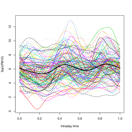
Figure 2: A plot of 175 daily curves $x_{t}(u)$, $1\leq t\leq 175$, where $x_{t}(u)$ are the square-root transformed and detrended functional observations of PM10, based on 15 Fourier basis functions. The solid black line represents the sample mean curve $\hat{\mu}(u)$.

From those data, we computed the (estimated) first dynamic FPC score sequence $(\hat{Y}_{1t}^{\mathrm{dyn}}\colon~{}1\leq~{}t\leq~{}175)$. To this end, we centered the data at their empirical mean $\hat{\mu}(u)$, then implemented the procedure described in Section 4. We used the traditional Bartlett kernel $w(x)=1-|x|$ in (20) to obtain an estimator for the spectral density operator, with bandwidth $q=\lfloor{n}^{1/2}\rfloor=13$. More sophisticated estimation methods, as those proposed, for example, by Politis [29], of course can be considered; but they also depend on additional tuning parameters, still leaving much of the selection to the practitioner’s choice. From $\hat{\mathcal{F}}_{\theta}^{\mathbf{X}}$ we obtain the estimated filter elements $\hat{\phi}_{1\ell}$. It turns out that they fade away quite rapidly. In particular $\sum_{\ell=-10}^{10}\|\hat{\phi}_{1\ell}\|^{2}\approx 0.998$. Hence, for calculation of the scores in (21) it is justified to choose $L=10$. The five central filter elements $\hat{\phi}_{1\ell}(u)$, $\ell=-2,\ldots,2$, are plotted in Figure 3.

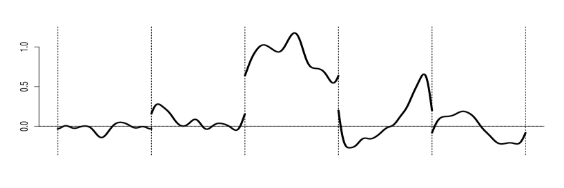
Figure 3: The five central filter elements $\hat{\phi}_{1,-2}(u),\ldots,\hat{\phi}_{1,2}(u)$ (from left to right).

Further components could be computed similarly, but for the purpose of demonstration we focus on one component only. In fact, the first dynamic FPC already explains about $80\%$ of the total variance, compared to the $73\%$ explained by the first static FPC. The latter was also computed, resulting in the static FPC score sequence $(\hat{Y}_{1t}^{\mathrm{stat}}\colon~{}1\leq~{}t\leq~{}175)$. Both sequences are shown in Figure 4, along with their differences.

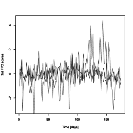
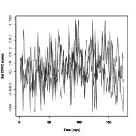
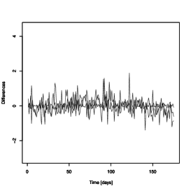
Figure 4: First static (left panel) and first dynamic (middle panel) FPC score sequences, and their differences (right panel).

Although based on entirely different ideas, the static and dynamic scores in Figure 4 (which, of course, are not loading the same functions) appear to be remarkably close to one another. The reason why the dynamic Karhunen-Loève expansion accounts for a significantly larger amount of the total variation is that, contrary to its static counterpart, it does not just involve the present observation.

To get more statistical insight into those results, let us consider the first static sample FPC, $\hat{v}_{1}(u)$, say, displayed in Figure 5.

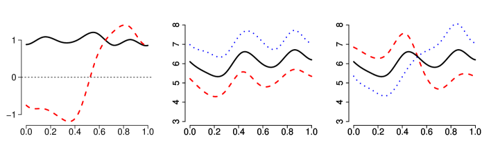
Figure 5: First static FPC $\hat{v}_{1}(u)$ (solid line), and second static FPC $\hat{v}_{2}(u)$ (dashed line) [left panel]. $\hat{\mu}(u)\pm\hat{v}_{1}(u)$ [middle panel] and $\hat{\mu}(u)\pm\hat{v}_{2}(u)$ [right panel] describe the effect of the first and second static FPC on the mean curve.

We see that $\hat{v}_{1}(u)\approx 1$ for all $u\in[0,1]$, so that the static FPC score $\hat{Y}_{1t}^{\mathrm{stat}}=\int_{0}^{1}(X_{t}(u)-\hat{\mu}(u))\hat{v}_{1}(u)du$  roughly coincides with the average deviation of $X_{t}(u)$ from the sample mean $\hat{\mu}(u)$: the effect of a large (small) first score corresponds to a large (small) daily average of $\sqrt{{\tt PM10}}$. In view of the similarity between $\hat{Y}_{1t}^{\mathrm{dyn}}$ and $\hat{Y}_{1t}^{\mathrm{stat}}$, it is possible to attribute the same interpretation to the dynamic FPC scores. However, regarding the dynamic Karhunen-Loève expansion, dynamic FPC scores should be interpreted sequentially. To this end, let us take advantage of the fact that $\sum_{\ell=-1}^{1}\|\hat{\phi}_{1\ell}\|^{2}\approx 0.92$. In the approximation by a single-term dynamic Karhunen-Loève expansion, we thus roughly have

$$X_{t}(u)\approx\hat{\mu}(u)+\sum_{\ell=-1}^{1}\hat{Y}_{1,t+\ell}^{\mathrm{dyn}}\hat{\phi}_{1\ell}(u).$$

This suggests studying the impact of triples $(\hat{Y}_{1,t-1}^{\mathrm{dyn}},\hat{Y}_{1t}^{\mathrm{dyn}},\hat{Y}_{1,t+1}^{\mathrm{dyn}})$ of consecutive scores on the pollution level of day $t$. We do this by adding the functions

$$\mathrm{eff}(\delta_{-1},\delta_{0},\delta_{1}):=\sum_{\ell=-1}^{1}\delta_{\ell}\hat{\phi}_{1\ell}(u),\quad\text{with}\quad\delta_{i}=\mathrm{const}\times\pm 1,\vspace{-1mm}$$

to the overall mean curve $\hat{\mu}(u)$. In Figure 6, we do this with $\delta_{i}=\pm 1$. For instance, the upper left panel shows $\hat{\mu}(u)+\mathrm{eff}(-1,-1,-1)$, corresponding to the impact of three consecutive small dynamic FPC scores. The result is a negative shift of the mean curve. If two small scores are followed by a large one (second panel from the left in top row), then the PM10 level increases as $u$ approaches 1. Since a large value of $\hat{Y}_{1,t+1}^{\mathrm{dyn}}$ implies a large average concentration of $\sqrt{\tt{PM10}}$ on day $t+1$, and since the pollution curves are highly correlated at the transition from day $t$ to day $t+1$, this should indeed be reflected by a higher value of $\sqrt{{\tt PM10}}$ towards the end of day $t$. Similar interpretations can be given for the other panels in Figure 6.

It is interesting to observe that, in this example, the first dynamic FPC seems to take over the roles of the first two static FPCs. The second static FPC (see Figure 5) indeed can be interpreted as an intraday trend effect; if the second static score of day $t$ is large (small), then $X_{t}(u)$ is increasing (decreasing) over $u\in[0,1]$. Since we are working with sequentially dependent data, we can get information about such a trend from future and past observations, too. Hence, roughly speaking, we have

$$\sum_{\ell=-1}^{1}\hat{Y}_{1,t+\ell}^{\mathrm{dyn}}\hat{\phi}_{1\ell}(u)\approx\sum_{m=1}^{2}\hat{Y}_{mt}^{\mathrm{stat}}\hat{v}_{m}(u).$$

This is exemplified in Figure 1 of Section 1, which shows the ten consecutive curves $x_{71}(u)-\hat{\mu}(u),\ldots,x_{80}(u)-\hat{\mu}(u)$ (left panel) and compares them to the single-term static (middle panel) and the single-term dynamic Karhunen-Loève expansions (right panel).

Figure 6: Mean curves $\hat{\mu}(u)$ (solid line) and $\hat{\mu}(u)+\mathrm{eff}(\delta_{-1},\delta_{0},\delta_{1})$, with $\delta_{i}=\pm 1$ (dashed).

6 Simulation study

In this simulation study, we compare the performance of dynamic FPCA with that of static FPCA for a variety of data-generating processes. For each simulated functional time series $(X_{t})$, where $X_{t}=X_{t}(u)$, $u\in[0,1]$, we compute the static and dynamic scores, and recover the approximating series $(\hat{X}_{t}^{\mathrm{stat}}(p))$ and $(\hat{X}_{t}^{\mathrm{dyn}}(p))$ that result from the static and dynamic Karhunen-Loève expansions, respectively, of order $p$. The performances of these approximations are measured in terms of the corresponding normalized mean squared errors (NMSE)

$$\sum_{t=1}^{n}\|X_{t}-\hat{X}_{t}^{\mathrm{stat}}(p)\|^{2}\Big{/}\sum_{t=1}^{n}\|X_{t}\|^{2}\quad\text{and}\quad\sum_{t=1}^{n}\|X_{t}-\hat{X}_{t}^{\mathrm{dyn}}(p)\|^{2}\Big{/}\sum_{t=1}^{n}\|X_{t}\|^{2}.$$

The smaller these quantities, the better the approximation.

Computations were implemented in R, along with the fda package. The data were simulated according to a functional AR(1) model $X_{n+1}=\Psi(X_{n})+\varepsilon_{n+1}$. In practice, this simulation has to be performed in finite dimension $d$, say. To this end, let $(v_{i})$, $i\in\mathbb{N}$ be the Fourier basis functions on $[0,1]$: for large $d$, due to the linearity of $\Psi$,

$$\langle X_{n+1},v_{j}\rangle=\langle\Psi(X_{n}),v_{j}\rangle+\langle\varepsilon_{n+1},v_{j}\rangle$$

$$\quad=\langle\Psi\big{(}\sum_{i=1}^{\infty}\langle X_{n},v_{i}\rangle v_{i}\big{)},v_{j}\rangle+\langle\varepsilon_{n+1},v_{j}\rangle\approx\sum_{i=1}^{d}\langle X_{n},v_{i}\rangle\langle\Psi(v_{i}),v_{j}\rangle+\langle\varepsilon_{n+1},v_{j}\rangle.$$

Hence, letting $\mathbf{X}_{n}=(\langle X_{n},v_{1}\rangle,\ldots,\langle X_{n},v_{d}\rangle)^{\prime}$ and $\boldsymbol{\varepsilon}_{n}=(\langle\varepsilon_{n+1},v_{1}\rangle,\ldots,\langle\varepsilon_{n+1},v_{d}\rangle)^{\prime}$, the first $d$ Fourier coefficients of $X_{n}$ approximately satisfy the VAR(1) equation$\mathbf{X}_{n+1}=\mathfrak{P}\mathbf{X}_{n}+\boldsymbol{\varepsilon}_{n},$ where $\mathfrak{P}=(\langle\Psi(v_{i}),v_{j}\rangle\colon 1\leq i,j\leq d)$. Based on this observation, we used a VAR(1) model for generating the first $d$ Fourier coefficients of the process $(X_{n})$. To obtain $\mathfrak{P}$, we generate a matrix $G=(G_{ij}\colon 1\leq i,j\leq d)$, where the $G_{ij}$’s are mutually independent $N(0,\psi_{ij})$, and then set $\mathfrak{P}:=\kappa{G}/{\|G\|}$. Different choices of $\psi_{ij}$ are considered. Since $\Psi$ is bounded, we have $\mathfrak{P}_{ij}\to 0$ as $i,j\to\infty$. For the operators $\Psi_{1}$, $\Psi_{2}$ and $\Psi_{3}$, we used $\psi_{ij}=(i^{2}+j^{2})^{-1/2}$, $\psi_{ij}=(i^{2/2}+j^{3/2})^{-1}$, and $\psi_{ij}=e^{-(i+j)}$, respectively. For $d$ and $\kappa$, we considered the values $d=15,31,51,101$ and $\kappa=0.1,0.3,0.6,0.9$. The noise $(\varepsilon_{t})$ is chosen as independent Gaussian and obtained as a linear combination of the functions $(v_{i}\colon 1\leq i\leq d)$ with independent zero-mean normal coefficients $(C_{i}\colon 1\leq i\leq d)$, such that $\mathrm{Var}(C_{i})=\exp((i-1)/10)$. With this approach, we generate $n=400$ observations. We then follow the methodology described in Section 4 and use the Barlett kernel in (20) for estimation of the spectral density operator. The tuning parameter $q$ is set equal to $\sqrt{n}=20$. A more sophisticated calibration probably can lead to even better results, but we also observed that moderate variations of $q$ do not fundamentally change our findings. The numerical integration for obtaining $\hat{\phi}_{mk}$ is performed on the basis of $1000$ equidistant integration points. In (21) we chose $L=\min(L^{\prime},60)$, where $L^{\prime}=\mathrm{argmin}_{j\geq 0}\sum_{-j\leq\ell\leq j}\|\hat{\phi}_{m\ell}\|^{2}\geq 0.99$. The limitation $L\leq 60$ is imposed to keep computation times moderate. Usually, convergence is relatively fast.

For each choice of $d$ and $\kappa$, the experiment as described above is repeated $200$ times. The mean and standard deviation of NMSE in different settings and with values $p=1,2,3,6$ are reported in Table 1. Results do not vary much among setups with $d\geq 31$, and thus in Table 1 we only present the cases $d=15$ and $d=101$.

We see that, in basically all settings, dynamic FPCA significantly outperforms static FPCA in terms of NMSE. As one can expect, the difference becomes more striking with increasing dependence coefficient $\kappa$. It is also interesting to observe that the variations of NMSE among the 200 replications is systematically smaller for the dynamic procedure.

Finally, it should be noted that, in contrast to the static PCA, the empirical version of our procedure is not “exact”, but is subject to small approximation errors. These approximation errors can stem from numerical integration (which is required in the calculation of $\hat{\phi}_{mk}$) and are also due to the truncation of the filters at some finite lag $L$ (see Section 4). Such little deviations do not matter in practice if a component explains a significant proportion of variance. If, however, the additional contribution of the higher-order component is very small, then it can happen that it doesn’t compensate a possible approximation error. This becomes visible in the setting $\Psi_{3}$ with 3 or 6 components, where for some constellations the NMSE for dynamic components is slightly larger than for the static ones.

			$1$ component		$2$ components		$3$ components		$6$ components
	$d$	$\kappa$	static	dynamic	static	dynamic	static	dynamic	static	dynamic
$\Psi_{1}$	15	0.1	0.697 (0.16)	0.637 (0.13)	0.546 (0.15)	0.447 (0.10)	0.443 (0.12)	0.325 (0.08)	0.256 (0.08)	0.138 (0.05)
		0.3	0.696 (0.16)	0.621 (0.14)	0.542 (0.15)	0.434 (0.11)	0.440 (0.13)	0.314 (0.08)	0.253 (0.08)	0.132 (0.05)
		0.6	0.687 (0.32)	0.571 (0.23)	0.526 (0.25)	0.392 (0.15)	0.423 (0.20)	0.283 (0.11)	0.240 (0.11)	0.119 (0.06)
		0.9	0.648 (0.76)	0.479 (0.47)	0.481 (0.56)	0.322 (0.29)	0.377 (0.43)	0.229 (0.20)	0.209 (0.22)	0.096 (0.09)
	101	0.1	0.805 (0.12)	0.740 (0.08)	0.708 (0.11)	0.587 (0.08)	0.642 (0.12)	0.478 (0.07)	0.519 (0.08)	0.274 (0.05)
		0.3	0.802 (0.13)	0.729 (0.11)	0.704 (0.12)	0.577 (0.09)	0.637 (0.11)	0.469 (0.08)	0.515 (0.10)	0.269 (0.05)
		0.6	0.792 (0.22)	0.690 (0.18)	0.689 (0.19)	0.545 (0.12)	0.619 (0.16)	0.441 (0.10)	0.495 (0.13)	0.252 (0.07)
		0.9	0.755 (0.66)	0.616 (0.45)	0.640 (0.50)	0.479 (0.31)	0.568 (0.40)	0.387 (0.23)	0.446 (0.34)	0.220 (0.15)
$\Psi_{2}$	15	0.1	0.524 (0.20)	0.491 (0.17)	0.355 (0.14)	0.306 (0.11)	0.263 (0.10)	0.208 (0.08)	0.129 (0.05)	0.082 (0.03)
		0.3	0.522 (0.21)	0.473 (0.18)	0.351 (0.16)	0.294 (0.12)	0.259 (0.12)	0.200 (0.08)	0.126 (0.06)	0.078 (0.04)
		0.6	0.507 (0.49)	0.413 (0.29)	0.331 (0.29)	0.255 (0.15)	0.240 (0.19)	0.174 (0.10)	0.114 (0.08)	0.068 (0.05)
		0.9	0.458 (1.15)	0.310 (0.59)	0.272 (0.64)	0.187 (0.32)	0.193 (0.41)	0.130 (0.21)	0.088 (0.17)	0.052 (0.09)
	101	0.1	0.585 (0.19)	0.549 (0.17)	0.436 (0.15)	0.378 (0.11)	0.356 (0.13)	0.282 (0.10)	0.240 (0.08)	0.146 (0.05)
		0.3	0.581 (0.21)	0.530 (0.18)	0.436 (0.12)	0.369 (0.11)	0.350 (0.13)	0.274 (0.09)	0.234 (0.10)	0.141 (0.06)
		0.6	0.564 (0.46)	0.469 (0.27)	0.405 (0.33)	0.321 (0.18)	0.323 (0.21)	0.242 (0.13)	0.212 (0.12)	0.125 (0.07)
		0.9	0.495 (1.06)	0.362 (0.59)	0.345 (0.68)	0.250 (0.39)	0.251 (0.58)	0.180 (0.34)	0.168 (0.26)	0.097 (0.14)
$\Psi_{3}$	15	0.1	0.367 (0.20)	0.344 (0.18)	0.134 (0.08)	0.127 (0.07)	0.049 (0.03)	0.054 (0.04)	0.002 (0.00)	0.017 (0.03)
		0.3	0.362 (0.24)	0.322 (0.17)	0.129 (0.09)	0.119 (0.07)	0.048 (0.03)	0.050 (0.04)	0.002 (0.00)	0.015 (0.03)
		0.6	0.334 (0.55)	0.253 (0.24)	0.113 (0.16)	0.097 (0.09)	0.041 (0.05)	0.040 (0.04)	0.002 (0.00)	0.011 (0.02)
		0.9	0.236 (1.12)	0.146 (0.43)	0.074 (0.28)	0.061 (0.16)	0.025 (0.08)	0.027 (0.07)	0.001 (0.00)	0.008 (0.04)
	101	0.1	0.366 (0.19)	0.344 (0.17)	0.134 (0.08)	0.127 (0.07)	0.049 (0.03)	0.054 (0.04)	0.002 (0.00)	0.017 (0.03)
		0.3	0.363 (0.25)	0.322 (0.18)	0.131 (0.10)	0.120 (0.07)	0.047 (0.03)	0.050 (0.04)	0.002 (0.00)	0.015 (0.03)
		0.6	0.325 (0.52)	0.251 (0.24)	0.113 (0.16)	0.098 (0.09)	0.040 (0.05)	0.040 (0.04)	0.002 (0.00)	0.011 (0.02)
		0.9	0.235 (1.05)	0.149 (0.43)	0.074 (0.28)	0.061 (0.16)	0.025 (0.09)	0.026 (0.07)	0.001 (0.00)	0.008 (0.04)

Table 1: Results of the simulations of Section 6. Bold numbers represent the mean of NMSE for dynamic and static procedures resulting from 200 simulation runs. The numbers in brackets show standard deviations multiplied by a factor 10. The values $\kappa$ give the size of $\|\Psi_{i}\|_{\mathcal{L}}$, $i=1,2,3$. We consider dimensions of the underlying models $d=15$ and $d=101$.

7 Conclusion

Functional principal component analysis is taking a leading role in the functional data literature. As an extremely effective tool for dimension reduction, it is useful for empirical data analysis as well as for many FDA-related methods, like functional linear models. A frequent situation in practice is that functional data are observed sequentially over time and exhibit serial dependence. This happens, for instance, when observations stem from a continuous-time process which is segmented into smaller units, e.g., days. In such cases, classical static FPCA still may be useful, but, in contrast to the i.i.d. setup, it does not lead to an optimal dimension-reduction technique.

In this paper, we propose a dynamic version of FPCA which takes advantage of the potential serial dependencies in the functional observations. In the special case of uncorrelated data, the dynamic FPC methodology reduces to the usual static one. But, in the presence of serial dependence, static FPCA is (quite significantly, if serial dependence is strong) outperformed.

This paper also provides (i) guidelines for practical implementation, (ii) a toy example with PM10 air pollution data, and (iii) a simulation study. Our empirical application brings empirical evidence that dynamic FPCs have a clear edge over static FPCs in terms of their ability to represent dependent functional data in small dimension. In the appendices, our results are cast into a rigorous mathematical framework, and we show that the proposed estimators of dynamic FPC scores are consistent.

Appendix A General methodology and proofs

In this subsection, we give a mathematically rigorous description of the methodology introduced in Section 3.1. We adopt a more general framework which can be specialized to the functional setup of Section 3.1. Throughout, $H$ denotes some (complex) separable Hilbert space equipped with norm $\|\cdot\|$ and inner product $\langle\cdot,\cdot\rangle$. We work in complex spaces, since our theory is based on a frequency domain analysis. Nevertheless, all our functional time series observations $X_{t}$ are assumed to be real-valued functions.

A.1 Fourier series in Hilbert spaces.

For $p\geq 1$, consider the space $L_{H}^{p}([-\pi,\pi])$, that is, the space of measurable mappings $x:[-\pi,\pi]\to H$ such that $\int_{-\pi}^{\pi}\|x(\theta)\|^{p}d\theta<~{}\infty$. Then, $\|x\|_{p}=(\frac{1}{2\pi}\int_{-\pi}^{\pi}\|x(\theta)\|^{p}d\theta)^{1/p}$ defines a norm. Equipped with this norm, $L_{H}^{p}([-\pi,\pi])$ is a Banach space, and for $p=2$, a Hilbert space with inner product

$$(x,y):=\frac{1}{2\pi}\int_{-\pi}^{\pi}\langle x(\theta),y(\theta)\rangle d\theta.$$

One can show (see e.g. [8, Lemma 1.4]) that, for any $x\in L_{H}^{1}([-\pi,\pi])$, there exists a unique element $I(x)\in H$ which satisfies

$$\int_{-\pi}^{\pi}\langle x(\theta),v\rangle d\theta=\langle I(x),v\rangle\quad\forall v\in H.$$ (24)

We define $\int_{-\pi}^{\pi}x(\theta)d\theta:=I(x)$.

For $x\in L_{H}^{2}([-\pi,\pi])$, define the $k$-th Fourier coefficient as

$$f_{k}:=\frac{1}{2\pi}\int_{-\pi}^{\pi}x(\theta)e^{-\mathbbm{i}k\theta}d\theta,\quad k\in\mathbb{Z}.$$ (25)

Below, we write $e_{k}$ for the function $\theta\mapsto e^{\mathbbm{i}k\theta}$, $\theta\in[-\pi,\pi]$.

Proposition 5.

Suppose $x\in L_{H}^{2}([-\pi,\pi])$ and define $f_{k}$ by equation (25). Then, the sequence $S_{n}:=\sum_{k=-n}^{n}f_{k}e_{k}$ has a mean square limit in $L_{H}^{2}([-\pi,\pi])$. If we denote the limit by $S$, then $x(\theta)=S(\theta)$ for almost all $\theta$.

Let us turn to the Fourier expansion of eigenfunctions $\varphi_{m}(\theta)$ used in the definition of the dynamic DPFCs. Eigenvectors are scaled to unit length: $\|\varphi_{m}(\theta)\|^{2}=1$. In order for $\varphi_{m}$ to belong to $L_{H}^{2}([-\pi,\pi])$, we additionally need measurability. Measurability cannot be taken for granted. This comes from the fact that $\|z\varphi_{m}(\theta)\|^{2}=1$ for all $z$ on the complex unit circle. In principle we could choose the “signs” $z=z(\theta)$ in an extremely erratic way, such that $\varphi_{m}(\theta)$ is no longer measurable. To exclude such pathological choices, we tacitly impose in the sequel that versions of $\varphi_{m}(\theta)$ have been chosen in a “smooth enough way”, to be measurable.

Now we can expand the eigenfunctions $\varphi_{m}(\theta)$ in a Fourier series in the sense explained above:

$$\varphi_{m}=\sum_{\ell\in\mathbb{Z}}\phi_{m\ell}e_{\ell}\quad\text{with}\quad\phi_{m\ell}=\frac{1}{2\pi}\int_{-\pi}^{\pi}\varphi_{m}(s)e^{-\mathbbm{i}\ell s}ds.$$

The coefficients $\phi_{m\ell}$ thus defined yield the definition (11) of dynamic FPCs. In the special case $H=L^{2}([0,1])$, $\phi_{m\ell}=\phi_{m\ell}(u)$ satisfies by (24)

$$\int_{0}^{1}\phi_{m\ell}(u)v(u)du =\frac{1}{2\pi}\int_{-\pi}^{\pi}\int_{0}^{1}\varphi_{m}(u|s)v(u)due^{-\mathbbm{i}\ell s}ds$$

$$=\int_{0}^{1}\left(\frac{1}{2\pi}\int_{-\pi}^{\pi}\varphi_{m}(u|s)e^{-\mathbbm{i}\ell s}ds\right)v(u)du\quad\forall v\in H.$$

This implies that $\phi_{m\ell}(u)=\frac{1}{2\pi}\int_{-\pi}^{\pi}\varphi_{m}(u|s)e^{-\mathbbm{i}\ell s}ds$ for almost all $u\in[0,1]$, which is in line with the definition given in (10). Furthermore, (9) follows directly from Proposition 5.

A.2 The spectral density operator

Assume that the $H$-valued process $(X_{t}\colon t\in\mathbb{Z})$ is stationary with lag $h$ autocovariance operator $C_{h}^{X}$ and spectral density operator

$$\mathcal{F}^{X}_{\theta}:=\frac{1}{2\pi}\sum_{h\in\mathbb{Z}}C_{h}^{X}e^{-\mathbbm{i}h\theta}.\vspace{-1mm}$$ (26)

Let $\mathcal{S}(H,H^{\prime})$ be the set of Hilbert-Schmidt operators mapping from $H$ to $H^{\prime}$ (both assumed to be separable Hilbert spaces). When $H=H^{\prime}$ and when it is clear which space $H$ is meant, we sometimes simply write $\mathcal{S}$. With the Hilbert-Schmidt norm $\|\cdot\|_{\mathcal{S}(H,H^{\prime})}$ this defines again a separable Hilbert space, and so does $L_{\mathcal{S}(H,H^{\prime})}^{2}([-\pi,\pi])$. We will impose that the series in (26) converges in $L_{\mathcal{S}(H,H)}^{2}([-\pi,\pi])$: we then say that $(X_{t})$ possesses a spectral density operator.

Remark 3.

It follows that the results of the previous section can be applied. In particular we may deduce that $C_{k}^{X}=\int_{-\pi}^{\pi}\mathcal{F}_{\theta}^{X}e^{\mathbbm{i}k\theta}d\theta$.

A sufficient condition for convergence of (26) in $L^{2}_{\mathcal{S}(H,H)}([-\pi,\pi])$ is assumption (6). Then, it can be easily shown that the operator $\mathcal{F}^{X}_{\theta}$ is self-adjoint, non-negative definite and Hilbert-Schmidt. Below, we introduce a weak dependence assumption established in [18], from which we can derive a sufficient condition for (6).

Definition 3 ($L^{p}$–$m$–approximability).

A random $H$–valued sequence $(X_{n}\colon n\in\mathbb{Z})$ is called $L^{p}$–$m$–approximable if it can be represented as $X_{n}=f(\delta_{n},\delta_{n-1},\delta_{n-2},...)$, where the $\delta_{i}$’s are i.i.d. elements taking values in some measurable space $S$ and $f$ is a measurable function $f:S^{\infty}\rightarrow H$. Moreover, if $\delta^{\prime}_{1},\delta^{\prime}_{2},...$ are independent copies of $\delta_{1},\delta_{2},...$ defined on the same measurable space $S$, then, for

$$X_{n}^{(m)}:=f(\delta_{n},\delta_{n-1},\delta_{n-2},...,\delta_{n-m+1},\delta^{\prime}_{n-m},\delta^{\prime}_{n-m-1},...),$$

we have

$$\sum_{m=1}^{\infty}(E\|X_{m}-X_{m}^{(m)}\|^{p})^{1/p}<\infty.$$ (27)

Hörmann and Kokoszka [18] show that this notion is widely applicable to linear and non-linear functional time series. One of its main advantages is that it is a purely moment-based dependence measure that can be easily verified in many special cases.

Proposition 6.

Assume that $(X_{t})$ is $L^{2}$–$m$–approximable. Then (6) holds and the operators $\mathcal{F}_{\theta}^{X}$, $\theta\in[-\pi,\pi]$, are trace-class.

Instead of Assumption (6), Panaretos and Tavakoli [27] impose for the definition of a spectral density operator summability of $C_{h}^{X}$ in Schatten 1-norm, that is, $\sum_{h\in\mathbb{Z}}\|C_{h}^{X}\|_{\mathcal{T}}<\infty$. Under such slightly more stringent assumption, it immediately follows that the resulting spectral operator is trace-class. The verification of convergence may, however, be a bit delicate. At least, we could not find a simple criterion as in Proposition 6.

Proposition 7.

Let $\mathcal{F}_{\theta}^{X}$ be the spectral density operator of a stationary sequence $(X_{t})$ for which the summability condition (6) holds. Let $\lambda_{1}(\theta)\geq\lambda_{2}(\theta)\geq\cdots$ denote its eigenvalues and $\varphi_{m}(\theta)$ be the corresponding eigenfunctions. Then, (a) the functions $\theta\mapsto\lambda_{m}(\theta)$ are continuous; (b) if we strengthen (6) into the more stringent condition $\sum_{h\in\mathbb{Z}}|h|\|C_{h}^{X}\|_{\mathcal{S}}<~{}\infty,$ the $\lambda_{m}(\theta)$’s are Lipschitz-continuous functions of $\theta$; (c) assuming that $(X_{t})$ is real-valued, for each $\theta\in[-\pi,\pi]$, $\lambda_{m}(\theta)=\lambda_{m}(-\theta)$ and $\varphi_{m}(\theta)=\overline{\varphi_{m}(-\theta)}$.

Let $\overline{x}$ be the conjugate element of $x$, i.e. $\langle x,z\rangle=\langle z,\overline{x}\rangle$ for all $z\in H$. Then $x$ is real-valued iff $x=\overline{x}$.

Remark 4.

Since $\varphi_{m}(\theta)$ is Hermitian, it immediately follows that $\phi_{m\ell}=\overline{\phi_{m\ell}},$ implying that the dynamic FPCs are real if the process $(X_{t})$ is.

A.3 Functional filters

Computation of dynamic FPCs requires applying time-invariant functional filters to the process $(X_{t})$. Let $\boldsymbol{\Psi}=(\Psi_{k}\colon k\in\mathbb{Z})$ be a sequence of linear operators mapping the separable Hilbert space $H$ to the separable Hilbert space $H^{\prime}$. Let $B$ be the backshift or lag operator, defined by $B^{k}X_{t}:=X_{t-k}$, $k\in\mathbb{Z}$. Then the functional filter $\Psi(B):=\sum_{k\in\mathbb{Z}}\Psi_{k}B^{k}$, when applied to the sequence $(X_{t})$, produces an output series $(Y_{t})$ in $H^{\prime}$ via

$$Y_{t}=\Psi(B)X_{t}=\sum_{k\in\mathbb{Z}}\Psi_{k}(X_{t-k}).$$ (28)

Call $\boldsymbol{\Psi}$ the sequence of filter coefficients, and, in the style of the scalar or vector time series terminology, call

$$\Psi_{\theta}=\Psi(e^{-\mathbbm{i}\theta})=\sum_{k\in\mathbb{Z}}\Psi_{k}e^{-\mathbbm{i}k\theta}$$ (29)

the frequency response function of the filter $\Psi(B)$. Of course, series (28) and (29) only have a meaning if they converge in an appropriate sense. Below we use the following technical lemma.

Proposition 8.

Suppose that $(X_{t})$ is a stationary sequence in $L_{H}^{2}$ and possesses a spectral density operator satisfying  $\sup_{\theta}\mathrm{tr}(\mathcal{F}_{\theta}^{X})<\infty$. Consider a filter $(\Psi_{k})$ such that $\Psi_{\theta}$ converges in $L^{2}_{\mathcal{S}(H,H^{\prime})}([-\pi,\pi])$, and suppose that $\sup_{\theta}\|\Psi_{\theta}\|_{\mathcal{S}(H,H^{\prime})}<\infty$. Then,

1. the series $Y_{t}:=\sum_{k\in\mathbb{Z}}\Psi_{k}(X_{t-k})$ converges in $L^{2}_{H^{\prime}}$;

2. $(Y_{t})$ possesses the spectral density operator $\mathcal{F}_{\theta}^{Y}=\Psi_{\theta}\mathcal{F}_{\theta}^{X}(\Psi_{\theta})^{*}$;

3. $\sup_{\theta}\mathrm{tr}(\mathcal{F}_{\theta}^{Y})<\infty$.

In particular, the last proposition allows for iterative applications. If $\sup_{\theta}\mathrm{tr}(\mathcal{F}_{\theta}^{X})<~{}\infty$ and $\Psi_{\theta}$ satisfies the above properties, then analogue results apply to the output $Y_{t}$. This is what we are using in the proofs of Theorems 1 and 2.

A.4 Proofs for Section 3

To start with, observe that Propositions 1 and 3 directly follow from Proposition 8. Part (a) of Proposition 2 also has been established in the previous Section (see Remark 4), and part (b) is immediate. Thus, we can proceed to the proof of Theorems 1 and 2.

Proof of Theorems 1 and 2.

Assume we have filter coefficients $\boldsymbol{\Psi}=(\Psi_{k}\colon k\in\mathbb{Z})$ and $\boldsymbol{\Upsilon}=(\Upsilon_{k}\colon k\in\mathbb{Z})$, where $\Psi_{k}:H\to\mathbb{C}^{p}$ and $\Upsilon_{k}:\mathbb{C}^{p}\to H$ both belong to the class $\mathcal{C}$. If $(X_{t})$ and $(Y_{t})$ are $H$-valued and $\mathbb{C}^{p}$-valued processes, respectively, then there exist elements $\psi_{mk}$ and $\upsilon_{mk}$ in $H$ such that

$$\Psi(B)(X_{t})=\sum_{k\in\mathbb{Z}}\left(\langle X_{t-k},\psi_{1k}\rangle,\ldots,\langle X_{t-k},\psi_{pk}\rangle\right)^{\prime}\vspace{-2mm}$$

and

$$\Upsilon(B)(Y_{t})=\sum_{\ell\in\mathbb{Z}}\sum_{m=1}^{p}Y_{t+\ell,m}\upsilon_{m\ell}.$$

Hence, the $p$-dimensional reconstruction of $X_{t}$ in Theorem 2 is of the form

$$\sum_{m=1}^{p}\tilde{X}_{mt}=\Upsilon(B)[\Psi(B)X_{t}]=:\Upsilon\Psi(B)X_{t}.$$

Since $\boldsymbol{\Psi}$ and $\boldsymbol{\Upsilon}$ are required to belong to $\mathcal{C}$, we conclude from Proposition 8 that the processes $Y_{t}:=\Psi(B)X_{t}$ and $\tilde{X}_{t}=\Upsilon(B)Y_{t}$ are mean-square convergent and possess a spectral density operator. Letting $\psi_{m}(\theta)=\sum_{k\in\mathbb{Z}}\psi_{mk}e^{\mathbbm{i}k\theta}$ and $\upsilon_{m}(\theta)=\sum_{\ell\in\mathbb{Z}}\upsilon_{m\ell}e^{\mathbbm{i}\ell\theta}$, we obtain, for $x\in H$ and $y=(y_{1},\ldots,y_{m})^{\prime}\in\mathbb{C}^{p}$, that the frequency response functions $\Psi_{\theta}$ and $\Upsilon_{\theta}$ satisfy

$$\Psi_{\theta}(x)=\sum_{k\in\mathbb{Z}}\left(\langle x,\psi_{1k}\rangle,\ldots,\langle x,\psi_{pk}\rangle\right)^{\prime}e^{-\mathbbm{i}k\theta}=\left(\langle x,\psi_{1}(\theta)\rangle,\ldots,\langle x,\psi_{p}(\theta)\rangle\right)^{\prime}\vspace{-2mm}$$

and

$$\Upsilon_{\theta}(y)=\sum_{\ell\in\mathbb{Z}}\sum_{m=1}^{p}y_{m}\upsilon_{m\ell}e^{-\mathbbm{i}\ell\theta}=\sum_{m=1}^{p}y_{m}\upsilon_{m}(-\theta).$$

Consequently,

$$\Upsilon_{\theta}\Psi_{\theta}=\sum_{m=1}^{p}\upsilon_{m}(-\theta)\otimes\psi_{m}(\theta).$$ (30)

Now, using Proposition 8, it is readily verified that, for $Z_{t}:=X_{t}-\Upsilon\Psi(B)X_{t}$, we obtain the spectral density operator

$$\mathcal{F}^{Z}_{\theta}=\left(\tilde{\mathcal{F}}^{X}_{\theta}-\Upsilon_{\theta}\Psi_{\theta}\tilde{\mathcal{F}}^{X}_{\theta}\right)\left(\tilde{\mathcal{F}}^{X}_{\theta}-\tilde{\mathcal{F}}^{X}_{\theta}\Psi^{*}_{\theta}\Upsilon_{\theta}^{*}\right),$$ (31)

where $\tilde{\mathcal{F}}^{X}_{\theta}$ is such that $\tilde{\mathcal{F}}^{X}_{\theta}\tilde{\mathcal{F}}^{X}_{\theta}=\mathcal{F}^{X}_{\theta}.$

Using Lemma 5,

$$E\|X_{t}-\Upsilon\Psi(B)X_{t}\|^{2}=\int_{-\pi}^{\pi}\mathrm{tr}(\mathcal{F}_{\theta}^{Z})\,d\theta=\int_{-\pi}^{\pi}\Big{\|}\tilde{\mathcal{F}}^{X}_{\theta}-\Upsilon_{\theta}\Psi_{\theta}\tilde{\mathcal{F}}^{X}_{\theta}\Big{\|}_{\mathcal{S}}^{2}d\theta.$$ (32)

Clearly, (32) is minimized if we minimize the integrand for every fixed $\theta$ under the constraint that $\Upsilon_{\theta}\Psi_{\theta}$ is of the form (30). Employing the eigendecomposition $\mathcal{F}^{X}_{\theta}=\sum_{m\geq 1}\lambda_{m}(\theta)\varphi_{m}(\theta)\otimes\varphi_{m}(\theta)$, we infer that

$$\tilde{\mathcal{F}}^{X}_{\theta}=\sum_{m\geq 1}\sqrt{\lambda_{m}(\theta)}\varphi_{m}(\theta)\otimes\varphi_{m}(\theta).\vspace{-2mm}$$

The best approximating operator of rank $p$ to $\tilde{\mathcal{F}}_{\theta}^{X}$ is the operator

$$\tilde{\mathcal{F}}^{X}_{\theta}(p)=\sum_{m=1}^{p}\sqrt{\lambda_{m}(\theta)}\varphi_{m}(\theta)\otimes\varphi_{m}(\theta),$$

which is obtained if we choose $\Upsilon_{\theta}\Psi_{\theta}=\sum_{m=1}^{p}\varphi_{m}(\theta)\otimes\varphi_{m}(\theta)$ and hence

$$\psi_{m}(\theta)=\varphi_{m}(\theta)\quad\text{and}\quad\upsilon_{m}(\theta)=\varphi_{m}(-\theta).$$

Consequently, by Proposition 5, we get

$$\psi_{mk}=\frac{1}{2\pi}\int_{-\pi}^{\pi}\varphi_{m}(s)e^{-\mathbbm{i}ks}ds\quad\text{and}\quad\upsilon_{mk}=\frac{1}{2\pi}\int_{-\pi}^{\pi}\varphi_{m}(-s)e^{-\mathbbm{i}ks}ds=\psi_{m,-k}.$$

With this choice, it is clear that $\Upsilon\Psi(B)X_{t}=\sum_{m=1}^{p}X_{mt}$ and

$$E\|X_{t}-\sum_{m=1}^{p}X_{mt}\|^{2}=\int_{-\pi}^{\pi}\Big{\|}\tilde{\mathcal{F}}^{X}_{\theta}-\tilde{\mathcal{F}}^{X}_{\theta}(p)\Big{\|}_{\mathcal{S}}^{2}d\theta=\int_{-\pi}^{\pi}\sum_{m>p}\lambda_{m}(\theta)d\theta;$$

the proof of Theorem 2 follows.

Turning to Theorem 1, observe that, by the monotone convergence theorem, the last integral tends to zero if $p\to\infty$, which completes the proof of Theorem 1. ∎

Appendix B Large sample properties

For the proof of Theorem 3, let us show that $E|Y_{mt}-\hat{Y}_{mt}|\to 0$ as $n\to\infty$.

Fixing $L\geq 1$,

$$E|Y_{mt}-\hat{Y}_{mt}| \leq E\bigg{|}\mathop{\sum}\limits_{j\in\mathbb{Z}}\langle X_{t-j},\phi_{mj}\rangle-\mathop{\sum}\limits_{j=-L}^{L}\langle X_{t-j},\hat{\phi}_{mj}\rangle\bigg{|}$$

$$\leq E\bigg{|}\mathop{\sum}\limits_{j=-L}^{L}\langle X_{t-j},\phi_{mj}-\hat{\phi}_{mj}\rangle\bigg{|}+E\bigg{|}\mathop{\sum}\limits_{|j|>L}\langle X_{t-j},\phi_{mj}\rangle\bigg{|},$$ (33)

and the result follows if each summand in (33) converges to zero, which we prove in the two subsequent lemmas. For notational convenience, we often suppress the dependence on the sample size $n$; all limits below, however, are taken as $n\to\infty$.

Lemma 2.

If $L=L(n)\to\infty$ sufficiently slowly, then, under Assumptions $B.1$–$B.3$, we have that $\Big{|}\mathop{\sum}\limits_{|j|\leq L}\langle X_{k-j},\phi_{mj}-\hat{\phi}_{mj}\rangle\Big{|}=o_{P}(1).$

Proof.

The triangle and Cauchy-Schwarz inequalities yield

$$\Big{|}\mathop{\sum}\limits_{|j|\leq L}\langle X_{k-j},\phi_{mj}-\hat{\phi}_{mj}\rangle\Big{|} \leq\mathop{\sum}\limits_{j=-L}^{L}\|X_{k-j}\|\|\phi_{mj}-\hat{\phi}_{mj}\|$$

$$\leq\max_{j\in\mathbb{Z}}\|\phi_{mj}-\hat{\phi}_{mj}\|\mathop{\sum}\limits_{j=-L}^{L}\|X_{k-j}\|.$$

Let $\hat{c}_{m}(\theta):=\langle\phi_{m}(\theta),\hat{\phi}_{m}(\theta)\rangle/|\langle\phi_{m}(\theta),\hat{\phi}_{m}(\theta)\rangle|$. Jensen’s inequality and the triangular inequality imply that, for any $j\in\mathbb{Z}$,

$$2\pi\|\phi_{mj}-\hat{\phi}_{mj}\| =\Big{\|}\int_{-\pi}^{\pi}(\varphi_{m}(\theta)-\hat{\varphi}_{m}(\theta))e^{\mathbbm{i}j\theta}d\theta\Big{\|}\leq\int_{-\pi}^{\pi}\|\varphi_{m}(\theta)-\hat{\varphi}_{m}(\theta)\|d\theta$$

$$\leq\int_{-\pi}^{\pi}\|\varphi_{m}(\theta)-\hat{c}_{m}(\theta)\hat{\varphi}_{m}(\theta)\|d\theta+\int_{-\pi}^{\pi}|1-\hat{c}_{m}(\theta)|d\theta$$

$$=:Q_{1}+Q_{2}.$$

By Lemma 3.2 in [18], we have

$$Q_{1}\leq\int_{-\pi}^{\pi}\frac{8}{|\alpha_{m}(\theta)|^{2}}\|\mathcal{F}_{\theta}^{X}-\hat{\mathcal{F}}_{\theta}^{X}\|_{\mathcal{S}}\wedge 2\ d\theta.$$

By Assumption B.2, $\alpha_{m}(\theta)$ has only finitely many zeros, $\theta_{1},\ldots,\theta_{K}$, say. Let $\delta_{\varepsilon}(\theta):=[\theta-\varepsilon,\theta+\varepsilon]$ and $A(m,\varepsilon):=\bigcup_{i=1}^{K}\delta_{\varepsilon}(\theta_{i})$. By definition, the Lebesgue measure of this set is $|A(m,\varepsilon)|\leq 2K\varepsilon$. Define $M_{\varepsilon}$ such that

$$M_{\varepsilon}^{-1}=\min\{\alpha_{m}(\theta)\ |\ \theta\in[-\pi,\pi]\backslash A(m,\varepsilon)\}.$$

By continuity of $\alpha_{m}(\theta)$ (see Proposition 7), we have $M_{\varepsilon}<\infty$, and thus

$$\int_{-\pi}^{\pi}\frac{8}{|\alpha_{m}(\theta)|^{2}}\|\mathcal{F}_{\theta}^{X}-\hat{\mathcal{F}}_{\theta}^{X}\|\wedge 2d\theta\leq 4K\varepsilon+8M_{\varepsilon}^{2}\int_{-\pi}^{\pi}\|\mathcal{F}_{\theta}^{X}-\hat{\mathcal{F}}_{\theta}^{X}\|d\theta=:B_{n,\varepsilon}.$$

By Assumption B.1, there exists a sequence $\varepsilon_{n}\rightarrow 0$ such that $B_{n,\varepsilon_{n}}\rightarrow 0$ in probability, which entails $Q_{1}=o_{P}(1)$. Note that this also implies

$$\int_{-\pi}^{\pi}\big{|}\langle\varphi_{m}(\theta),v\rangle-\hat{c}_{m}(\theta)\langle\hat{\varphi}_{m}(\theta),v\rangle\big{|}d\theta=o_{P}(1).$$ (34)

Turning to $Q_{2}$, suppose that $Q_{2}$ is not $o_{P}(1)$ Then, there exists $\varepsilon>0$ and $\delta>0$ such that ,for infinitely many $n$, $P(Q_{2}\geq\varepsilon)\geq\delta$. Set

$$F=F_{n}:=\left\{\theta\in[-\pi,\pi]\colon|\hat{c}_{m}(\theta)-1|\geq\frac{\varepsilon}{4\pi}\right\}.$$

One can easily show that, on the set $\{Q_{2}\geq\varepsilon\}$, we have $\lambda(F)>\varepsilon/4$. Clearly, $|\hat{c}_{m}(\theta)-1|\geq{\varepsilon}/{4\pi}$ implies that $\hat{c}_{m}(\theta)=e^{\mathbbm{i}z(\theta)}$ with $z(\theta)\in[-\pi/2,-\varepsilon^{\prime}]\cup[\varepsilon^{\prime},\pi/2]$, for some small enough $\varepsilon^{\prime}$. Then the left-hand side in (34) is bounded from below by

$$\int_{F}\big{|}\langle\varphi_{m}(\theta),v\rangle-\hat{c}_{m}(\theta)\langle\hat{\varphi}_{m}(\theta),v\rangle\big{|}d\theta$$

$$\quad=\int_{F}\left(\langle(\varphi_{m}(\theta),v\rangle-\cos(z(\theta)\langle\hat{\varphi}_{m}(\theta),v\rangle)^{2}+(\sin^{2}(z(\theta))\langle\hat{\varphi}_{m}(\theta),v\rangle^{2}\right)^{1/2}d\theta.$$ (35)

Write $F:=F^{\prime}\cup F^{\prime\prime}$, where

$$F^{\prime} :=F\cap\left\{\theta\colon|\langle\varphi_{m}(\theta),v\rangle-\cos(z(\theta))\langle\hat{\varphi}_{m}(\theta),v\rangle\big{|}\geq\frac{\langle\varphi_{m}(\theta),v\rangle}{2}\right\}\quad\text{and}$$

$$F^{\prime\prime} :=F\cap\left\{\theta\colon|\langle\varphi_{m}(\theta),v\rangle-\cos(z(\theta))\langle\hat{\varphi}_{m}(\theta),v\rangle\big{|}<\frac{\langle\varphi_{m}(\theta),v\rangle}{2}\right\}.$$

On $F^{\prime}$, the integrand (35) is greater than or equal to $\langle\varphi_{m}(\theta),v\rangle/2$. On $F^{\prime\prime}$ the inequality $\cos(z(\theta))\langle\hat{\varphi}_{m}(\theta),v\rangle>\langle\varphi_{m}(\theta),v\rangle/2$ holds, and consequently

$$\langle\hat{\varphi}_{m}(\theta),v\rangle|\sin(z(\theta))| >\frac{\langle\varphi_{m}(\theta),v\rangle}{2}|\sin(z(\theta))|$$

$$>\frac{\langle\varphi_{m}(\theta),v\rangle}{\pi}|z(\theta)|\geq\frac{\langle\varphi_{m}(\theta),v\rangle}{\pi}\varepsilon^{\prime}.$$

Altogether, this yields that the integrand in (35) is larger than or equal to $\langle\varphi_{m}(\theta),v\rangle\varepsilon^{\prime}/\pi$. Now, it is easy to see that, due to Assumption B.3, (34) cannot hold. This leads to a contradiction.

Thus, we can conclude that $\max_{j\in\mathbb{Z}}\|\phi_{mj}-\hat{\phi}_{mj}\|=o_{P}(1)$, so that, for sufficiently slowly growing $L$, we also have $L\,\max_{j\in\mathbb{Z}}\|\phi_{mj}-\hat{\phi}_{mj}\|=o_{P}(1)$. Consequently,

$$\Bigg{|}\mathop{\sum}\limits_{|j|\leq L}\langle X_{k-j},\phi_{mj}-\hat{\phi}_{mj}\rangle\Bigg{|} =o_{P}(1)\times\left(L^{-1}\mathop{\sum}\limits_{j=-L}^{L}\|X_{k-j}\|\right).$$ (36)

It remains to show that $L^{-1}\mathop{\sum}\limits_{j=-L}^{L}\|X_{k-j}\|=O_{P}(1)$. By the weak stationarity assumption, we have $E\|X_{k}\|^{2}=E\|X_{1}\|^{2}$, and hence, for any $x>0$,

$$P\bigg{(}L^{-1}\mathop{\sum}\limits_{j=-L}^{L}\|X_{k-j}\|>x\bigg{)}\leq\frac{\sum_{k=-L}^{L}E\|X_{k}\|}{Lx}\leq\frac{3\sqrt{E\|X_{1}\|^{2}}}{x}.$$

∎

Lemma 3.

Let $L=L(n)\to\infty$. Then, under condition (6), we have

$$\Bigg{|}\mathop{\sum}\limits_{|j|>L}\langle X_{k-j},\phi_{mj}\rangle\Bigg{|}=o_{P}(1).$$

Proof.

This is immediate from Proposition 3, part (a). ∎

Turning to the proof of Proposition 4, we first establish the following lemma, which an extension to lag-$h$ autocovariance operators of a consistency result from [18] on the empirical covariance operator. Define, for $|h|<n$,

$$\hat{C}_{h}=\frac{1}{n}\sum_{k=1}^{n-h}X_{k+h}\otimes X_{k},\quad h\geq 0,\quad\text{and}\quad\hat{C}_{h}=\hat{C}_{-h},\quad h<0.$$

Lemma 4.

Assume that $(X_{t}:t\in\mathbb{Z})$ is an $L^{4}$-$m$-approximable series. Then, for all $|h|<n$, $E\|\hat{C}_{h}-C_{h}\|_{\mathcal{S}}\leq U\sqrt{{(|h|\vee 1)}/{n}},$ where the constant $U$ neither depends on $n$ nor on $h$.

Proof of Proposition 4.

By the triangle inequality,

$$2\pi\|\mathcal{F}_{\theta}^{X}-\mathcal{\hat{F}}_{\theta}^{X}\|_{\mathcal{S}}=\Bigg{\|}\mathop{\sum}\limits_{k\in\mathbb{Z}}C_{h}e^{-\mathbbm{i}h\theta}-\mathop{\sum}\limits_{h=-q}^{q}\bigg{(}1-\frac{|h|}{q}\bigg{)}\hat{C}_{h}e^{-\mathbbm{i}h\theta}\Bigg{\|}_{\mathcal{S}}$$

$$\qquad\leq\Bigg{\|}\mathop{\sum}\limits_{h=-q}^{q}\bigg{(}1-\frac{|h|}{q}\bigg{)}(C_{h}-\hat{C}_{h})e^{-\mathbbm{i}h\theta}\Bigg{\|}_{\mathcal{S}}$$

$$\qquad\ \ \ +\Bigg{\|}\frac{1}{q}\mathop{\sum}\limits_{h=-q}^{q}|h|C_{h}e^{-\mathbbm{i}h\theta}\Bigg{\|}_{\mathcal{S}}+\Bigg{\|}\mathop{\sum}\limits_{|h|>q}C_{h}e^{-\mathbbm{i}h\theta}\Bigg{\|}_{\mathcal{S}}$$

$$\qquad\leq\mathop{\sum}\limits_{h=-q}^{q}\bigg{(}1-\frac{|h|}{q}\bigg{)}\|C_{h}-\hat{C}_{h}\|_{\mathcal{S}}+\frac{1}{q}\mathop{\sum}\limits_{h=-q}^{q}|h|\|C_{h}\|_{\mathcal{S}}+\mathop{\sum}\limits_{|h|>q}\|C_{h}\|_{\mathcal{S}}.$$

The last two terms tend to $0$ by condition (6) and Kronecker’s lemma. For the first term we may use Lemma 4. Taking expectations, we obtain that, for some $U_{1}$,

$$\mathop{\sum}\limits_{h=-q}^{q}\bigg{(}1-\frac{|h|}{q}\bigg{)}E\|C_{h}-\hat{C}_{h}\|_{\mathcal{S}}\leq U_{1}\frac{q^{3/2}}{\sqrt{n}}.\vspace{-1mm}$$

Note that the bound does not depend on $\theta$; hence $q^{3}=o(n)$ and condition (6) jointly imply that $\sup_{\theta\in[-\pi,\pi]}E\|\mathcal{F}_{\theta}^{X}-\mathcal{\hat{F}}_{\theta}^{X}\|_{\mathcal{S}}\to 0$ as $n\to\infty$. ∎

Appendix C Technical results and background

C.1 Linear operators

Consider the class $\mathcal{L}(H,H^{\prime})$ of bounded linear operators between two Hilbert spaces $H$ and $H^{\prime}$. For $\Psi\in\mathcal{L}(H,H^{\prime})$, the operator norm is defined as $\|\Psi\|_{\mathcal{L}}:=\sup_{\|x\|\leq 1}\|\Psi(x)\|$. The simplest operators can be defined via a tensor product $v\otimes w$; then $v\otimes w(z):=v\langle z,w\rangle$. Every operator $\Psi\in\mathcal{L}(H,H^{\prime})$ possesses an adjoint $\Psi^{*}\in\mathcal{L}(H^{\prime},H)$, which satisfies $\langle\Psi(x),y\rangle=\langle x,\Psi^{*}(y)\rangle$ for all $x\in H$ and $y\in H^{\prime}$. It holds that $\|\Psi^{*}\|_{\mathcal{L}}=\|\Psi\|_{\mathcal{L}}$. If $H=H^{\prime}$, then $\Psi$ is called self-adjoint if $\Psi=\Psi^{*}$. It is called non-negative definite if $\langle\Psi x,x\rangle\geq 0$ for all $x\in H$.

A linear operator $\Psi\in\mathcal{L}(H,H^{\prime})$ is said to be Hilbert-Schmidt if, for some orthonormal basis $(v_{k}\colon k\geq 1)$ of $H$, we have $\|\Psi\|_{\mathcal{S}}^{2}:=\sum_{k\geq 1}\|\Psi(v_{k})\|^{2}<\infty$. Then, $\|\Psi\|_{\mathcal{S}}$ defines a norm, the so-called Hilbert-Schmidt norm of $\Psi$, which bounds the operator norm $\|\Psi\|_{\mathcal{L}}\leq\|\Psi\|_{\mathcal{S}}$, and can be shown to be independent of the choice of the orthonormal basis. Every Hilbert-Schmidt operator is compact. The class of Hilbert-Schmidt operators between $H$ and $H^{\prime}$ defines again a separable Hilbert space with inner product $\langle\Psi,\Theta\rangle_{\mathcal{S}}:=\sum_{k\geq 1}\langle\Psi(v_{k}),\Theta(v_{k})\rangle$: denote this class by $\mathcal{S}(H,H^{\prime})$.

If $\Psi\in\mathcal{L}(H,H^{\prime})$ and $\Upsilon\in\mathcal{L}(H^{\prime\prime},H)$, then $\Psi\Upsilon$ is the operator mapping $x\in H^{\prime\prime}$ to $\Psi(\Upsilon(x))\in H^{\prime}$. Assume that $\Psi$ is a compact operator in $\mathcal{L}(H,H^{\prime})$ and let $(s^{2}_{j})$ be the eigenvalues of $(\Psi^{*})\Psi$. Then $\Psi$ is said to be trace class if $\|\Psi\|_{\mathcal{T}}:=\sum_{j\geq 1}s_{j}<\infty$. In this case, $\|\Psi\|_{\mathcal{T}}$ defines a norm, the so-called Schatten 1-norm. We have that $\|\Psi\|_{\mathcal{S}}\leq\|\Psi\|_{\mathcal{T}}$, and hence any trace-class operator is Hilbert-Schmidt. For self-adjoint non-negative operators, it holds that $\|\Psi\|_{\mathcal{T}}=\mathrm{tr}(\Psi):=\sum_{k\geq 1}\langle\Psi(v_{k}),v_{k}\rangle$. If $\tilde{\Psi}\tilde{\Psi}=\Psi$, then we have $\mathrm{tr}(\Psi)=\|\tilde{\Psi}\|_{\mathcal{S}}^{2}$.

For further background on the theory of linear operators we refer to [13].

C.2 Random sequences in Hilbert spaces

All random elements that appear in the sequel are assumed to be defined on a common probability space $(\Omega,\mathcal{A},P)$. We write $X\in L_{H}^{p}(\Omega,\mathcal{A},P)$ (in short, $X\in L_{H}^{p}$) if $X$ is an $H$-valued random variable such that $E\|X\|^{p}<\infty$. Every element $X\in L_{H}^{1}$ possesses an expectation, which is the unique $\mu\in H$ satisfying $E\langle X,y\rangle=\langle\mu,y\rangle$ for all $y\in H$. Provided that $X$ and $Y$ are in $L_{H}^{2}$, we can define the cross-covariance operator as $C_{XY}:=E(X-\mu_{X})\otimes(Y-\mu_{Y})$, where $\mu_{X}$ and $\mu_{Y}$ are the expectations of $X$ and $Y$, respectively. We have that $\|C_{XY}\|_{\mathcal{T}}\leq E\|(X-\mu_{X})\otimes(Y-\mu_{Y})\|_{\mathcal{T}}=E\|X-\mu_{X}\|\|Y-\mu_{Y}\|$, and so these operators are trace-class. An important specific role is played by the covariance operator $C_{XX}$. This operator is non-negative definite and self-adjoint with $\mathrm{tr}(C_{XX})=E\|X-\mu_{X}\|^{2}$. An $H$-valued process $(X_{t})$ is called (weakly) stationary if $(X_{t})\in L_{H}^{2}$, and $EX_{t}$ and $C_{X_{t+h}X_{t}}$ do not depend on $t$. In this case, we write $C_{h}^{X}$, or shortly $C_{h}$, for $C_{X_{t+h}X_{t}}$ if it is clear to which process it belongs.

Many useful results on random processes in Hilbert spaces or more general Banach spaces are collected in Chapters 1 and 2 of [8].

C.3 Proofs for Appendix A

Proof of Proposition 5.

Letting $0<m<n$, note that

$$\|S_{n}-S_{m}\|_{2}^{2} =\bigg{(}\sum_{m\leq|k|\leq n}f_{k}e_{k},\sum_{m\leq|\ell|\leq n}f_{\ell}e_{\ell}\bigg{)}$$

$$=\frac{1}{2\pi}\int_{-\pi}^{\pi}\sum_{m\leq|k|\leq n}\sum_{m\leq|\ell|\leq n}\langle f_{k},f_{\ell}\rangle e^{\mathbbm{i}(k-\ell)\theta}d\theta=\sum_{m\leq|k|\leq n}\|f_{k}\|^{2}.$$

To prove the first statement, we need to show that $(S_{n})$ defines a Cauchy sequence in $L_{H}^{2}([-\pi,\pi])$, which follows if we show that $\sum_{k\in\mathbb{Z}}\|f_{k}\|^{2}<\infty$. We use the fact that, for any $v\in H$, the function $\langle x(\theta),v\rangle$ belongs to $L^{2}([-\pi,\pi])$. Then, by Parseval’s identity and (24), we have, for any $v\in H$,

$$\frac{1}{2\pi}\int_{-\pi}^{\pi}|\langle x(\theta),v\rangle|^{2}d\theta =\sum_{k\in\mathbb{Z}}\left(\frac{1}{2\pi}\int_{-\pi}^{\pi}\langle x(s),v\rangle e^{-\mathbbm{i}ks}ds\right)^{2}=\sum_{k\in\mathbb{Z}}|\langle f_{k},v\rangle|^{2}.$$

Let $(v_{k}\colon k\geq 1)$ be an orthonormal basis of $H$. Then, by the last result and Parseval’s identity again, it follows that

$$\|x\|_{2}^{2} =\frac{1}{2\pi}\int_{-\pi}^{\pi}\sum_{\ell\geq 1}|\langle x(\theta),v_{\ell}\rangle|^{2}d\theta=\frac{1}{2\pi}\sum_{\ell\geq 1}\int_{-\pi}^{\pi}|\langle x(\theta),v_{\ell}\rangle|^{2}d\theta$$

$$=\sum_{\ell\geq 1}\sum_{k\in\mathbb{Z}}|\langle f_{k},v_{\ell}\rangle|^{2}=\sum_{k\in\mathbb{Z}}\|f_{k}\|^{2}.$$

As for the second statement, we conclude from classical Fourier analysis results that, for each $v\in H$,

$$\lim_{n\to\infty}\frac{1}{2\pi}\int_{-\pi}^{\pi}\left(\langle x(\theta),v\rangle-\sum_{k=-n}^{n}\left(\frac{1}{2\pi}\int_{-\pi}^{\pi}\langle x(s),v\rangle e^{-\mathbbm{i}ks}ds\right)e^{\mathbbm{i}k\theta}\right)^{2}d\theta=0.\vspace{-1mm}$$

Now, by definition of $S_{n}$, this is equivalent to

$$\lim_{n\to\infty}\frac{1}{2\pi}\int_{-\pi}^{\pi}\left\langle x(\theta)-S_{n}(\theta),v\right\rangle^{2}d\theta=0,\quad\forall v\in H.\vspace{-1mm}$$

Combined with the first statement of the proposition and

$$\int_{-\pi}^{\pi}\left\langle x(\theta)-S(\theta),v\right\rangle^{2}d\theta \leq 2\int_{-\pi}^{\pi}\left\langle x(\theta)-S_{n}(\theta),v\right\rangle^{2}d\theta$$

$$\quad+2\|v\|^{2}\int_{-\pi}^{\pi}\|S_{n}(\theta)-S(\theta)\|^{2}d\theta,$$

this implies that

$$\frac{1}{2\pi}\int_{-\pi}^{\pi}\left\langle x(\theta)-S(\theta),v\right\rangle^{2}d\theta=0,\quad\forall v\in H.$$ (37)

Let $(v_{i})$, $i\in\mathbb{N}$ bee an orthonormal basis of $H$, and define

$$A_{i}:=\{\theta\in[-\pi,\pi]\colon\left\langle x(\theta)-S(\theta),v_{i}\right\rangle\neq 0\}.\vspace{-2mm}$$

By (37), we have that $\lambda(A_{i})=0$ ($\lambda$ denotes the Lebesgue measure), and hence $\lambda(A)=~{}0$ for $A=\cup_{i\geq 1}A_{i}$. Consequently, since $(v_{i})$ define an orthonormal basis, for any $\theta\in[-\pi,\pi]\setminus A$, we have $\langle x(\theta)-S(\theta),v\rangle=0$ for all $v\in H$, which in turn implies that $x(\theta)-S(\theta)=0$. ∎

Proof of Proposition 6.

Without loss of generality, we assume that $EX_{0}=0$. Since $X_{0}$ and $X_{h}^{(h)}$, $h\geq 1$, are independent,

$$\|C_{h}^{X}\|_{\mathcal{S}}=\|EX_{0}\otimes(X_{h}-X_{h}^{(h)})\|_{\mathcal{S}}\leq(E\|X_{0}\|^{2})^{1/2}(E\|X_{h}-X_{h}^{(h)}\|^{2})^{1/2}.$$

The first statement of the proposition follows.

Let $\theta$ be fixed. Since $\mathcal{F}_{\theta}^{X}$ is non-negative and self-adjoint, it is trace class if and only if

$$\mathrm{tr}(\mathcal{F}_{\theta}^{X})=\sum_{m\geq 1}\langle\mathcal{F}_{\theta}^{X}(v_{m}),v_{m}\rangle<\infty$$ (38)

for some orthonormal basis $(v_{m})$ of $H$. The trace can be shown to be independent of the choice of the basis. Define $V_{n,\theta}=(2\pi n)^{-1/2}\sum_{k=1}^{n}X_{k}e^{\mathbbm{i}k\theta}$ and note that, by stationarity,

$$\mathcal{F}_{n,\theta}^{X}:=EV_{n,\theta}\otimes V_{n,\theta}=\frac{1}{2\pi}\sum_{|h|<n}\left(1-\frac{|h|}{n}\right)EX_{0}\otimes X_{-h}e^{-\mathbbm{i}h\theta}.$$

It is easily verified that the operators $\mathcal{F}_{n,\theta}^{X}$ again are non-negative and self-adjoint. Also note that, by the triangular inequality,

$$\|\mathcal{F}_{n,\theta}^{X}-\mathcal{F}_{\theta}^{X}\|_{\mathcal{S}}\leq\sum_{|h|<n}\frac{|h|}{n}\|C_{h}^{X}\|_{\mathcal{S}}+\sum_{|h|\geq n}\|C_{h}^{X}\|_{\mathcal{S}}.$$

By application of (6) and Kronecker’s lemma, it easily follows that the latter two terms converge to zero. This implies that $\mathcal{F}_{n,\theta}^{X}(v)$ converges in norm to $\mathcal{F}_{\theta}^{X}(v)$, for any $v\in H$.

Choose $v_{m}=\varphi_{m}(\theta)$. Then, by continuity of the inner product and Fatou’s lemma, we have

$$\sum_{m\geq 1}\langle\mathcal{F}_{\theta}^{X}(\varphi_{m}(\theta)),\varphi_{m}(\theta)\rangle =\sum_{m\geq 1}\liminf_{n\to\infty}\langle\mathcal{F}_{n,\theta}^{X}(\varphi_{m}(\theta)),\varphi_{m}(\theta)\rangle$$

$$\leq\liminf_{n\to\infty}\sum_{m\geq 1}\langle\mathcal{F}_{n,\theta}^{X}(\varphi_{m}(\theta)),\varphi_{m}(\theta)\rangle.$$

Using the fact that the $\mathcal{F}_{n,\theta}^{X}$’s are self-adjoint and non-negative, we get

$$\sum_{m\geq 1}\langle\mathcal{F}_{n,\theta}^{X}(\varphi_{m}(\theta)),\varphi_{m}(\theta)\rangle =\mathrm{tr}(\mathcal{F}_{n,\theta}^{X})=E\|V_{n}\|^{2}$$

$$=\frac{1}{2\pi}\sum_{|h|<n}\left(1-\frac{|h|}{n}\right)E\langle X_{0},X_{h}\rangle e^{-\mathbbm{i}h\theta}.$$

Since $|E\langle X_{0},X_{h}\rangle|=|E\langle X_{0},X_{h}-X_{h}^{(h)}\rangle|$, by the Cauchy-Schwarz inequality,

$$\sum_{h\in\mathbb{Z}}|E\langle X_{0},X_{h}\rangle|\leq\sum_{h\in\mathbb{Z}}(E\|X_{0}\|^{2})^{1/2}(E(X_{h}-X_{h}^{(h)})^{2})^{1/2}<\infty,$$

and thus the dominated convergence theorem implies that

$$\mathrm{tr}(\mathcal{F}_{\theta}^{X})\leq\sum_{h\in\mathbb{Z}}|E\langle X_{0},X_{h}\rangle|<\infty,$$ (39)

which completes he proof.∎

Proof of Proposition 7.

We have (see e.g. [13], p. 186) that the dynamic eigenvalues are such that $|\lambda_{m}(\theta)-\lambda_{m}(\theta^{\prime})|\leq\|\mathcal{F}_{\theta}^{X}-\mathcal{F}_{\theta^{\prime}}^{X}\|_{\mathcal{S}}.$ Now,

$$\|\mathcal{F}_{\theta}^{X}-\mathcal{F}_{\theta^{\prime}}^{X}\|_{\mathcal{S}}\leq\sum_{h\in\mathbb{Z}}\|C_{h}^{X}\|_{\mathcal{S}}|e^{-\mathbbm{i}h\theta}-e^{-\mathbbm{i}h\theta^{\prime}}|.$$

The summability condition (6) implies continuity, hence part (a) of the proposition. The fact that $|e^{-\mathbbm{i}h\theta}-e^{-\mathbbm{i}h\theta^{\prime}}|\leq|h||\theta-\theta^{\prime}|$ yields part (b). To prove (c), observe that

$$\lambda_{m}(\theta)\varphi_{m}(\theta)=\mathcal{F}_{\theta}^{X}(\varphi_{m}(\theta))=\frac{1}{2\pi}\sum_{h\in\mathbb{Z}}EX_{h}\langle\varphi_{m}(\theta),X_{0}\rangle e^{-\mathbbm{i}h\theta}$$

for any $\theta\in[-\pi,\pi]$. Since the eigenvalues $\lambda_{m}(\theta)$ are real, we obtain, by computing the complex conjugate of the above equalities,

$$\lambda_{m}(\theta)\overline{\varphi_{m}(\theta)}=\frac{1}{2\pi}\sum_{h\in\mathbb{Z}}EX_{h}\langle\overline{\varphi_{m}(\theta)},X_{0}\rangle e^{\mathbbm{i}h\theta}=\mathcal{F}_{-\theta}^{X}(\overline{\varphi_{m}(\theta)}).$$

This shows that $\lambda_{m}(\theta)$ and $\overline{\varphi_{m}(\theta)}$ are eigenvalue and eigenfunction of $\mathcal{F}^{X}_{-\theta}$ and they must correspond to a pair $(\lambda_{n}(-\theta),\varphi_{n}(-\theta))$; (c) follows. ∎

Lemma 5.

Let $(Z_{t})$ be a stationary sequence in $L_{H}^{2}$ with spectral density $\mathcal{F}^{Z}_{\theta}$. Then,

$$\int_{-\pi}^{\pi}\mathrm{tr}(\mathcal{F}_{\theta}^{Z})d\theta=\mathrm{tr}\Big{(}\int_{-\pi}^{\pi}\mathcal{F}_{\theta}^{Z}d\theta\Big{)}=\mathrm{tr}(C_{0}^{Z})=E\|Z_{t}\|^{2}.$$

Proof.

Let $\mathcal{S}=\mathcal{S}(H,H)$. Note that $\int_{-\pi}^{\pi}\mathcal{F}_{\theta}^{Z}d\theta=\mathrm{I}\mathcal{F}^{Z}$ if and only if

$$\langle\mathrm{I}\mathcal{F}^{Z},V\rangle_{\mathcal{S}}=\int_{-\pi}^{\pi}\langle\mathcal{F}_{\theta}^{Z},V\rangle_{\mathcal{S}}\,d\theta\quad\text{for all }V\in\mathcal{S}.$$ (40)

For some orthonormal basis $(v_{k})$ define $V_{N}=\sum_{k=1}^{N}v_{k}\otimes v_{k}$. Then (40) implies that

$$\mathrm{tr}(\mathrm{I}\mathcal{F}^{Z}) =\lim_{N\to\infty}\sum_{k=1}^{N}\langle\mathrm{I}\mathcal{F}^{Z}(v_{k}),v_{k}\rangle=\lim_{N\to\infty}\langle\mathrm{I}\mathcal{F}^{Z},V_{N}\rangle_{\mathcal{S}}$$

$$=\lim_{N\to\infty}\int_{-\pi}^{\pi}\langle\mathcal{F}_{\theta}^{Z},V_{N}\rangle_{\mathcal{S}}d\theta=\lim_{N\to\infty}\int_{-\pi}^{\pi}\sum_{k=1}^{N}\langle\mathcal{F}_{\theta}^{Z}(v_{k}),v_{k}\rangle\,d\theta.$$

Since $\mathcal{F}_{\theta}^{Z}$ is non-negative definite for any $\theta$, the monotone convergence theorem allows to interchange the limit with the integral. ∎

Proof of Proposition 8.

(i) Define $Y_{t}^{r,s}:=\sum_{r<|k|\leq s}\Psi_{k}(X_{t-k})$ and the related transfer operator $\Psi^{r,s}_{\theta}:=\sum_{r<|k|\leq s}\Psi_{k}e^{-\mathbbm{i}k\theta}$. We also use $Y_{t}^{s}=\Psi_{0}(X_{t})+Y_{t}^{0,s}$ and $\Psi^{s}_{\theta}=\Psi_{0}+\Psi^{0,s}_{\theta}$. Since $Y_{t}^{r,s}$ is a finite sum, it is obviously in $L^{2}_{H^{\prime}}$. Also, the finite number of filter coefficients makes it easy to check that $(Y_{t}^{r,s}\colon t\in\mathbb{Z})$ is stationary and has spectral density operator $\mathcal{F}_{\theta}^{Y^{r,s}}=\Psi_{\theta}^{r,s}\mathcal{F}_{\theta}^{X}(\Psi_{\theta}^{r,s})^{*}$. By the previous lemma we have

$$E\|Y_{t}^{r,s}\|^{2} =\int_{-\pi}^{\pi}\mathrm{tr}(\mathcal{F}_{\theta}^{Y_{t}^{r,s}})d\theta=\int_{-\pi}^{\pi}\mathrm{tr}(\Psi_{\theta}^{r,s}\mathcal{F}_{\theta}^{X}(\Psi_{\theta}^{r,s})^{*})d\theta$$

$$\leq\int_{-\pi}^{\pi}\|\Psi_{\theta}^{r,s}\|^{2}_{\mathcal{S}(H,H^{\prime})}\mathrm{tr}(\mathcal{F}_{\theta}^{X})d\theta.$$

Now, it directly follows from the assumptions that $(Y_{t}^{s}\colon s\geq 1)$ defines a Cauchy sequence in $L^{2}_{H^{\prime}}$. This proves (i).

Next, remark that by our assumptions $\Psi_{\theta}\mathcal{F}_{\theta}^{X}(\Psi_{\theta})^{*}\in L^{2}_{\mathcal{S}(H^{\prime},H^{\prime})}([-\pi,\pi])$. Hence, by the results in Appendix A.1,

$$\sum_{|h|\leq r}\frac{1}{2\pi}\int_{-\pi}^{\pi}\Psi_{u}\mathcal{F}_{u}^{X}(\Psi_{u})^{*}e^{\mathbbm{i}hu}du\,e^{-\mathbbm{i}h\theta}\to\Psi_{\theta}\mathcal{F}_{\theta}^{X}(\Psi_{\theta})^{*}\quad\text{as }r\to\infty,$$

where convergence is in $L^{2}_{\mathcal{S}(H^{\prime},H^{\prime})}([-\pi,\pi])$. We prove that $\Psi_{\theta}\mathcal{F}_{\theta}^{X}(\Psi_{\theta})^{*}$ is the spectral density operator of $(Y_{t})$. This is the case if $\frac{1}{2\pi}\int_{-\pi}^{\pi}\Psi_{u}\mathcal{F}_{u}^{X}(\Psi_{u})^{*}e^{\mathbbm{i}hu}du=C_{h}^{Y}$. For the approximating sequences $(Y_{t}^{s}\colon t\in\mathbb{Z})$ we know from (i) and Remark 3 that

$$\frac{1}{2\pi}\int_{-\pi}^{\pi}\Psi_{u}^{s}\mathcal{F}_{u}^{X}(\Psi_{u}^{s})^{*}e^{\mathbbm{i}hu}du=C_{h}^{Y^{s}}.$$

Routine arguments show that under our assumptions $\|C_{h}^{Y^{s}}-C_{h}^{Y}\|_{\mathcal{S}(H^{\prime},H^{\prime})}\to 0$ and

$$\left\|\int_{-\pi}^{\pi}\left(\Psi_{u}\mathcal{F}_{u}^{X}(\Psi_{u})^{*}-\Psi_{u}^{s}\mathcal{F}_{u}^{X}(\Psi_{u}^{s})^{*}\right)e^{\mathbbm{i}hu}du\right\|_{\mathcal{S}(H^{\prime},H^{\prime})}\to 0,\quad(s\to\infty).$$

Part (ii) of the proposition follows, hence also part (iii). ∎

Proof of Lemma 4.

Let us only consider the case $h\geq 0$. Define $X_{n}^{(r)}$ as the $r$-dependent approximation of $(X_{n})$ provided by Definition 3. Observe that

$$nE\big{\|}\hat{C}_{h}-C_{h}\big{\|}_{\mathcal{S}}^{2}=nE\left\|\frac{1}{n}\sum\limits_{k=1}^{n-h}Z_{k}\right\|_{\mathcal{S}}^{2},$$

where $Z_{k}=X_{k+h}\otimes X_{k}-C_{h}$. Set $Z_{k}^{(r)}=X_{k+h}^{(r)}\otimes X_{k}^{(r)}-C_{h}$. Stationarity of $(Z_{k})$ implies

$$nE\left\|\frac{1}{n}\sum\limits_{k=1}^{n-h}Z_{k}\right\|_{\mathcal{S}}^{2} =\sum\limits_{|r|<n-h}\left(1-\frac{|r|}{n}\right)E\langle Z_{0},Z_{r}\rangle_{\mathcal{S}}$$

$$\leq\sum\limits_{r=-h}^{h}|E\langle Z_{0},Z_{r}\rangle_{\mathcal{S}}|+2\sum\limits_{r=h+1}^{\infty}|E\langle Z_{0},Z_{r}\rangle_{\mathcal{S}}|,$$ (41)

while the Cauchy-Schwarz inequality yields

$$|E\langle Z_{0},Z_{r}\rangle_{\mathcal{S}}|\leq E|\langle Z_{0},Z_{r}\rangle_{\mathcal{S}}|\leq\sqrt{E{\|Z_{0}\|_{\mathcal{S}}^{2}}E{\|Z_{r}\|_{\mathcal{S}}^{2}}}=E{\|Z_{0}\|_{\mathcal{S}}^{2}}.$$

Furthermore, from $\|X_{h}\otimes X_{0}\|=\|X_{h}\|\|X_{0}\|$, we deduce

$$E\|Z_{0}\|_{\mathcal{S}}^{2}=E\|X_{0}\|^{2}\|X_{h}\|^{2}\leq\left(E\|X_{0}\|^{4}\right)^{1/2}<\infty.$$

Consequently, we can bound the first sum in (41) by $(2h+1)\left(E\|X_{0}\|^{4}\right)^{1/2}$. For the second term in (41), we obtain, by independence of $Z_{r}^{(r-h)}$ and $Z_{0}$, that

$$|E\langle Z_{0},Z_{r}\rangle_{\mathcal{S}}|=|E\langle Z_{0},Z_{r}-Z_{r}^{(r-h)}\rangle_{\mathcal{S}}|\leq(E\|Z_{0}\|_{\mathcal{S}}^{2})^{1/2}(E\|Z_{r}-Z_{r}^{(r-h)}\|_{\mathcal{S}}^{2})^{1/2}.$$

To conclude, it suffices to show that $\sum_{r=1}^{\infty}(E\|Z_{r}-Z_{r}^{(r-h)}\|_{\mathcal{S}}^{2})^{1/2}\leq M<\infty$, where the bound $M$ is independent of $h$. Using an inequality of the type $|ab-cd|^{2}\leq 2|a|^{2}|b-d|^{2}+2|d|^{2}|a-c|^{2}$, we obtain

$$E\|Z_{r}-Z_{r}^{(r-h)}\|_{\mathcal{S}}^{2}=E\|X_{r}\otimes X_{r+h}-X_{r}^{(r-h)}\otimes X_{r+h}^{(r-h)}\|_{\mathcal{S}}^{2}$$

$$\qquad\leq 2E\|X_{r}\|^{2}\|X_{r+h}-X_{r+h}^{(r-h)}\|^{2}+2E\|X_{r+h}^{(r-h)}\|^{2}\|X_{r}-X_{r}^{(r-h)}\|^{2}$$

$$\qquad\leq 2(E\|X_{r}\|^{4})^{1/2}(E\|X_{r+h}-X_{r+h}^{(r-h)}\|^{4})^{1/2}$$

$$\qquad\quad+2(E\|X_{r+h}^{(r-h)}\|^{4})^{1/2}(E\|X_{r}-X_{r}^{(r-h)}\|^{4})^{1/2}.$$

Note that $E\|X_{r}\|^{4}=E\|X_{r+h}^{(r-h)}\|^{4}=E\|X_{0}\|^{4}$ and

$$E\|X_{r+h}-X_{r+h}^{(r-h)}\|^{4}=E\|X_{r}-X_{r}^{(r-h)}\|^{4}=E\|X_{0}-X_{0}^{(r-h)}\|^{4}.$$

Altogether we get

$$E\|Z_{r}-Z_{r}^{(r-h)}\|_{\mathcal{S}}^{2}\leq 4(E\|X_{0}\|^{4})^{1/2}(E\|X_{0}-X_{0}^{(r-h)}\|^{4})^{1/2}.$$

Hence, $L^{4}$-$m$-approximability implies that $\sum_{r=h+1}^{\infty}|E\langle Z_{0},Z_{r}\rangle_{\mathcal{S}}|$ converges and is uniformly bounded over $0\leq h<n$. ∎

References

• [1] Aue, A., Dubart Norinho, D. and Hörmann, S. (2014), On the prediction of functional time series, J. Amer. Statist. Assoc. (forthcoming).
• [2] Aston, J.A.D. and Kirch, C. (2011), Estimation of the distribution of change-points with application to fMRI data, Technical Report, University of Warwick, Centre for Research in Statistical Methodology, 2011.
• [3] Benko, M., Härdle, W. and Kneip, A. (2009), Common functional principal components, The Annals of Statistics 37, 1–34.
• [4] Berkes, I., Gabrys, R., Horváth, L. and Kokoszka, P.(2009), Detecting changes in the mean of functional observations, J. Roy. Statist. Soc. Ser. B, 71, 927–946.
• [5] Besse, P. and Ramsay, J. O. (1986), Principal components analysis of sampled functions, Psychometrika 51, 285–311.
• [6] Brillinger, D. R. (1981), Time Series: Data Analysis and Theory, Holden Day, San Francisco.
• [7] Brockwell, P. J. and Davis, R. A. (1981), Time Series: Theory and Methods, Springer, New York.
• [8] Bosq, D. (2000), Linear Processes in Function Spaces, Springer, New York.
• [9] Cardot, H., Ferraty, F. and Sarda, P. (1999), Functional linear model, Statist.& Probab. Lett. 45, 11–22.
• [10] Dauxois, J., Pousse, A. and Romain, Y. (1982), Asymptotic theory for the principal component analysis of a vector random function: Some applications to statistical inference, J. Multivariate Anal.  12, 136–154.
• [11] Ferraty, F. and Vieu, P. (2006), Nonparametric Functional Data Analysis, Springer, New York.
• [12] Gervini, D. (2007), Robust functional estimation using the median and spherical principal components, Biometrika 95, 587–600.
• [13] Gohberg, I., Goldberg, S. and Kaashoek, M. A. (2003), Basic Classes of Linear Operators, Birkhäuser.
• [14] Gokulakrishnan, P., Lawrence, P. D., McLellan, P. J. and Grandmaison, E. W. (2006), A functional-PCA approach for analyzing and reducing complex chemical mechanisms, Computers and Chemical Engineering 30, 1093–1101.
• [15] Hall, P. and Hosseini-Nasab, M. (2006), On properties of functional principal components analysis, J. Roy. Statist. Soc. Ser. B 68, 109–126.
• [16] Hall, P., Müller, H.-G. and Wang, J.-L. (2006), Properties of principal component methods for functional and longitudinal data analysis, The Annals of Statistics 34, 1493–1517.
• [17] Hörmann, S. and Kidziński, Ł. (2012), A note on estimation in Hilbertian linear models, Scand. J. Stat. (forthcoming).
• [18] Hörmann, S. and Kokoszka, P. (2010), Weakly dependent functional data, The Annals of Statistics 38, 1845–1884.
• [19] Hörmann, S. and Kokoszka, P. (2012), Functional Time Series, in Handbook of Statistics: Time Series Analysis-Methods and Applications, 157–186.
• [20] Hyndman, R. J. and Ullah, M. S. (2007), Robust forecasting of mortality and fertility rates: a functional data approach, Computational Statistics & Data Analysis 51, 4942–4956.
• [21] James, G.M., Hastie T. J. and Sugar, C. A. (2000), Principal component models for sparse functional data, Biometrika 87, 587–602.
• [22] Jolliffe, I.T. (2002), Principal Component Analysis, Springer, New York.
• [23] Karhunen, K. (1947), Über lineare Methoden in der Wahrscheinlichkeitsrechnung, Ann. Acad. Sci. Fennicae Ser. A. I. Math.-Phys. 37, 79.
• [24] Kneip, A. and Utikal, K. (2001), Inference for density families using functional principal components analysis, J. Amer. Statist. Assoc. 96, 519–531.
• [25] Locantore, N., Marron, J. S., Simpson, D. G., Tripoli, N., Zhang, J. T. and Cohen, K. L. (1999), Robust principal component analysis for functional data, Test 8, 1–73.
• [26] Loève, M. (1946), Fonctions aléatoires de second ordre, Revue Sci. 84, 195–206.
• [27] Panaretos, V. M. and Tavakoli, S. (2013a), Fourier analysis of stationary time series in function space, The Annals of Statistics 41, 568-603.
• [28] Panaretos, V. M. and Tavakoli, S. (2013b), Cramér-Karhunen-Loève representation and harmonic principal component analysis of functional time series, Stoch. Proc. Appl. 123, 2779-2807.
• [29] Politis, D. N. (2011), Higher-order accurate, positive semi-definite estimation of large-sample covariance and spectral density matrices, Econometric Theory 27, 703–744.
• [30] Ramsay, J. O. and Dalzell, C. J. (1991), Some tools for functional data analysis (with discussion), J. Roy. Statist. Soc. Ser. B 53, 539–572.
• [31] Ramsay, J. and Silverman, B. (2002), Applied Functional Data Analysis, Springer, New York.
• [32] Ramsay, J. and Silverman, B. (2005), Functional Data Analysis (2nd ed.), Springer, New York.
• [33] Reiss, P. T. and Ogden, R. T. Functional principal component regression and functional partial least squares, J. Amer. Statist. Assoc. 102, 984–996.
• [34] Silverman, B. (1996), Smoothed functional principal components analysis by choice of norm, The Annals of Statistics 24, 1–24.
• [35] Shumway, R. and Stoffer, D. (2006), Time Series Analysis and Its Applications (2nd ed.), Springer, New York.
• [36] Stadlober, E., Hörmann, S. and Pfleiler, B. (2008), Quality and performance of a PM10 daily forecasting model, Atmospheric Environment 42, 1098–1109.
• [37] Viviani, R., Grön, G. and Spitzer, M. (2005), Functional principal component analysis of fMRI data, Human Brain Mapping 24, 109–129.