HadISD: a quality-controlled global synoptic report database for selected variables at long-term stations from 1973–2011

Zusammenfassung

This paper describes the creation of HadISD: an automatically quality-controlled synoptic resolution dataset of temperature, dewpoint temperature, sea-level pressure, wind speed, wind direction and cloud cover from global weather stations for 1973–2011. The full dataset consists of over 6000 stations, with 3427 long-term stations deemed to have sufficient sampling and quality for climate applications requiring sub-daily resolution. As with other surface datasets, coverage is heavily skewed towards Northern Hemisphere mid-latitudes.

The dataset is constructed from a large pre-existing ASCII flatfile data bank that represents over a decade of substantial effort at data retrieval, reformatting and provision. These raw data have had varying levels of quality control applied to them by individual data providers. The work proceeded in several steps: merging stations with multiple reporting identifiers; reformatting to netCDF; quality control; and then filtering to form a final dataset. Particular attention has been paid to maintaining true extreme values where possible within an automated, objective process. Detailed validation has been performed on a subset of global stations and also on UK data using known extreme events to help finalise the QC tests. Further validation was performed on a selection of extreme events world-wide (Hurricane Katrina in 2005, the cold snap in Alaska in 1989 and heat waves in SE Australia in 2009). Some very initial analyses are performed to illustrate some of the types of problems to which the final data could be applied. Although the filtering has removed the poorest station records, no attempt has been made to homogenise the data thus far, due to the complexity of retaining the true distribution of high-resolution data when applying adjustments. Hence non-climatic, time-varying errors may still exist in many of the individual station records and care is needed in inferring long-term trends from these data.

This dataset will allow the study of high frequency variations of temperature, pressure and humidity on a global basis over the last four decades. Both individual extremes and the overall population of extreme events could be investigated in detail to allow for comparison with past and projected climate. A version-control system has been constructed for this dataset to allow for the clear documentation of any updates and corrections in the future.

The Integrated Surface Database (ISD) held at NOAA’s National Climatic Data Center is an archive of synoptic reports from a large number of global surface stations (Smith et al., 2011; Ame, 2004; see http://www.ncdc.noaa.gov/oa/climate/isd/index.php). It is a rich source of data useful for the study of climate variations, individual meteorological events and historical climate impacts. For example, these data have been applied to quantify precipitation frequency (Dai, 2001a) and its diurnal cycle (Dai, 2001b), diurnal variations in surface winds and divergence field (Dai and Deser, 1999), and recent changes in surface humidity (Dai, 2006; Willett et al., 2008), cloudiness (Dai et al., 2006) and wind speed (Peterson et al., 2011).

The collation of ISD, merging and reformatting to a single format from over 100 constituent sources and three major databanks represented a substantial and ground-breaking effort undertaken over more than a decade at NOAA NCDC. The database is updated in near real-time. A number of automated quality control (QC) tests are applied to the data that largely consider internal station series consistency and are geographically invariant in their application (i.e. threshold values are the same for all stations regardless of the local climatology). These procedures are briefly outlined in Ame (2004) and (Smith et al., 2011). The tests concentrate on the most widely used variables and consist of a mix of logical consistency checks and outlier type checks. Values are flagged rather than deleted. Automated checks are essential as it is impractical to manually check thousands of individual station records that could each consist of several tens of thousands of individual observations. It should be noted that the raw data in many cases have been previously quality controlled manually by the data providers, so the raw data are not necessarily completely raw for all stations.

The ISD database is non-trivial for the non-expert to access and use, as each station consists of a series of annual ASCII flatfiles (with each year being a separate directory) with each observation representing a row in a format akin to the synoptic reporting codes that is not immediately intuitive or amenable to easy machine reading (http://www1.ncdc.noaa.gov/pub/data/ish/ish-format-document.pdf). NCDC, however, provides access to the ISD database using a GIS interface. This does give the ability for users to select parameters and stations and output the results to a text file. Also, a subset of the ISD variables (air temperature, dewpoint temperature, sea level pressure, wind direction, wind speed, total cloud cover, one-hour accumulated liquid precipitation, six-hour accumulated liquid precipitation) is available as ISD-Lite in fixed-width format ASCII files. However, there has been no selection on data or station quality. In this paper we outline the steps undertaken to provide a new quality-controlled version, called HadISD, which is based on the raw ISD records, in netCDF format for selected variables for a subset of the stations with long records. This new dataset will allow the easy study of the behaviour of short-timescale climate phenomena in recent decades, with the subsequent comparison to past climates and future climate projections.

One of the primary uses of a sub-daily resolution database will be the characterisation of extreme events for specific locations, and so it is imperative that multiple, independent efforts be undertaken to assess the fundamental quality of individual observations. We also therefore undertake a new and comprehensive quality control of the ISD, based upon the raw holdings, which should be seen as complementary to that which already exists. In the same way that multiple independent homogenisation efforts have informed our understanding of true long-term trends in variables such as tropospheric temperatures (Thorne et al., 2011), numerous independent QC efforts will be required to fully understand changes in extremes. Arguably, in this context structural uncertainty (Thorne et al., 2005) in quality control choices will be as important as that in any homogenisation processes that were to be applied in ensuring an adequate portrayal of our true degree of uncertainty in extremes behaviour. Poorly applied quality control processes could certainly have a more detrimental effect than poor homogenisation processes. Too aggressive and the real tails are removed; too liberal and data artefacts remain to be misinterpreted by the unwary. As we are unable to know for certain whether a given value is truly valid, it is impossible to unambiguously determine the prevalence of type-I and type-II errors for any candidate QC algorithm. In this work, type-I errors occur when a good value is flagged, and type-II errors are when a bad value is not flagged.

Quality control is therefore an increasingly important aspect of climate dataset construction as the focus moves towards regional- and local-scale impacts and mitigation in support of climate services (Doherty et al., 2008). The data required to support these applications need to be at a much finer temporal and spatial resolution than is typically the case for most climate datasets, free of gross errors and homogenised in such a way as to retain the high as well as low temporal frequency characteristics of the record. Homogenisation at the individual observation level is a separate and arguably substantially more complex challenge. Here we describe solely the data preparation and QC. The methodology is loosely based upon that developed in Durre et al. (2010) for daily data from the Global Historical Climatology Network. Further discussion of the data QC problem, previous efforts and references can be found therein. These historical issues are not covered in any detail here.

Section 1 describes how stations that report under varying identifiers were combined, an issue that was found to be globally insidious and particularly prevalent in certain regions. Section 2 outlines selection of an initial set of stations for subsequent QC. Section 3 outlines the intra- and inter-station QC procedures developed and summarises their impact. We validate the final quality-controlled dataset in Sect. 4. Section LABEL:sec:finalselection briefly summarises the final selection of stations, and Sect. LABEL:sec:nomenclature describes our version numbering system. Section LABEL:sec:uses outlines some very simple analyses of the data to illustrate their likely utility, whilst Sect. LABEL:sec:summary concludes.

The final data are available through http://www.metoffice.gov.uk/hadobs/hadisd along with the large volume of process metadata that cannot reasonably be appended to this paper. The database covers 1973 to end-2011, because availability drops off substantially prior to 1973 (Willett et al., 2008). In future periodic updates are planned to keep the dataset up-to-date.

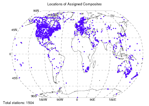
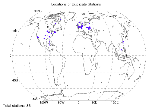
Abbildung 1: Top: locations of assigned composite stations from the ISD database before any station selection and filtering. Only 943 of these 1504 stations were passed into the QC process. Bottom: locations of 83 duplicated stations identified by the inter-station duplicate check (Sect. 3.1.1, test 1.)

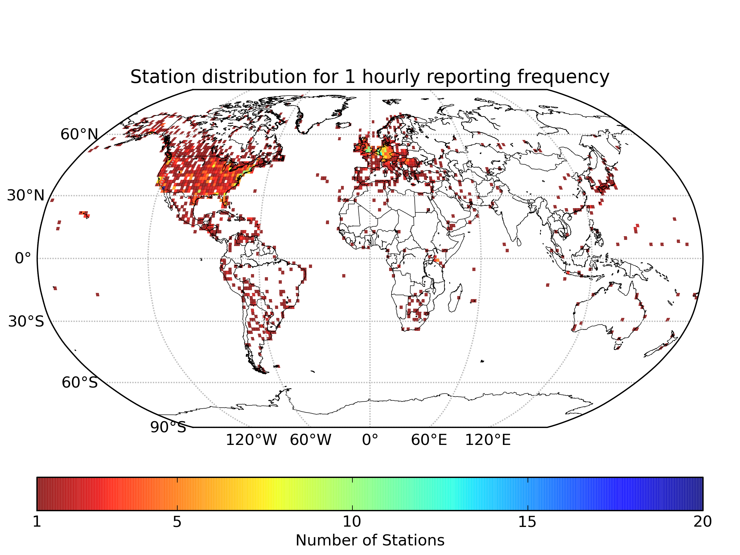
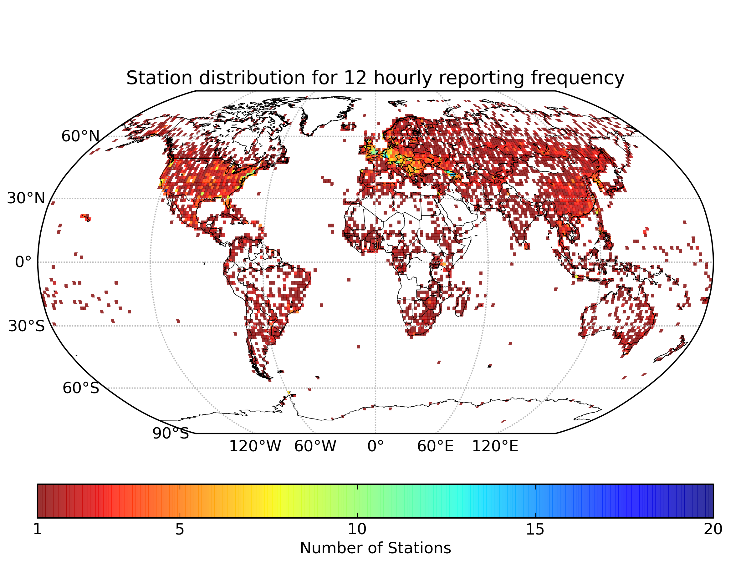
Abbildung 2: Station distributions for different minimum reporting frequencies for a 1976–2005 climatology period. For presentational purposes we show the number of stations within $1.5^{\circ}\times 1.5^{\circ}$ grid boxes. Hourly (top panel); 3-hourly (middle panel) and 12-hourly (bottom panel).

1 Compositing stations

The ISD database archives according to the station identifier (ID) appended to the report transmission, resulting in around 28 000 individual station IDs. Despite efforts by the ISD dataset creators, this causes issues for stations that have changed their reporting ID frequently or that have reported simultaneously under multiple IDs to different ISD source databanks (i.e. using a WMO identifier over the GTS and a national identifier to a local repository). Many such station records exist in multiple independent station files within the ISD database despite in reality being a single station record. In some regions, e.g. Canada and parts of Eastern Europe, WMO station ID changes have been ubiquitous, so compositing is essential for record completeness.

Tabelle 1: Hierarchical criteria for deciding whether given pairs of stations in the ISD master listing were potentially the same station and therefore needed assessing further. The final value arising for a given pair of stations is the sum of the values for all hierarchical criteria met, e.g. a station pair that agrees within the elevation and latitude/longitude bounds but for no other criteria will have a value of 7.

	Hierarchical
Criteria	criteria value
Reported elevation within 50 m	1
Latitude within 0.05∘	2
Longitude within 0.05∘	4
Same country	8
WMO identifier agrees and not missing, same country	16
USAF identifier agrees in first 5 numbers and not missing	32
Station name agrees and country either the same or missing	64
METAR (Civil aviation) station call sign agrees	128

Station location and ID information were read from the ISD station inventory, and the potential for station matches assessed by pairwise comparisons using a hierarchical scoring system (Table 1). The inventory is used instead of within data file location information as the latter had been found to be substantially more questionable (Neal Lott, personal communication, 2008). Scores are high for those elements which, if identical, would give high confidence that the stations are the same. For example it is highly implausible that a METAR call sign will have been recycled between geographically distinct stations. Station pairs that exceeded a total score of 14 are selected for further analysis (see Table 1). Therefore, a candidate pair for consideration must at an absolute minimum be close in distance and elevation and from the same country, or have the same ID or name. Several stations appeared in more than one unique pairing of potential composites. These cases were combined to form consolidated sets of potential matches. Some of these sets comprise as many as five apparently unique station IDs in the ISD database.

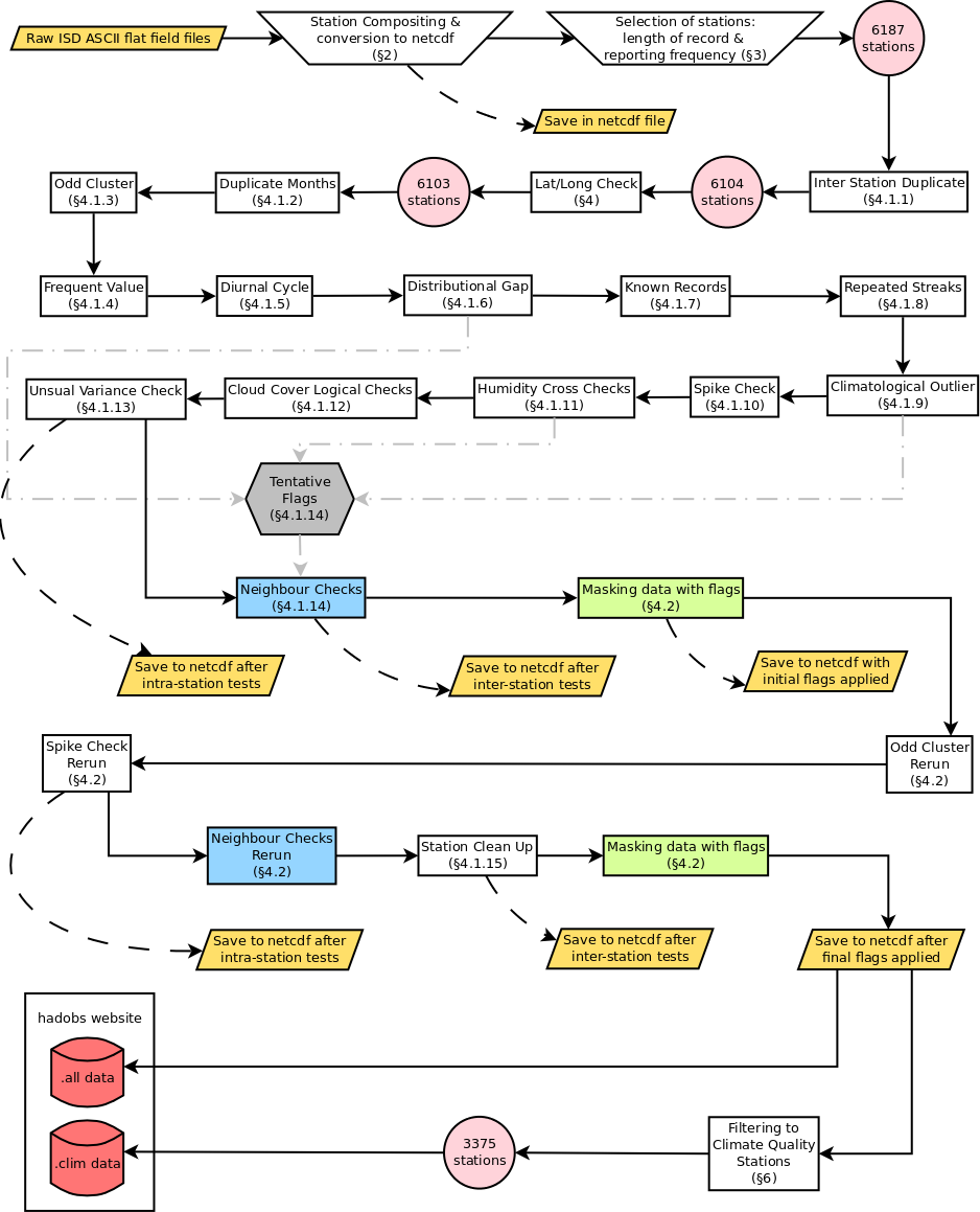
Abbildung 3: Flow diagram of the testing procedure. Final output is available on www.metoffice.gov.uk/hadobs/hadisd. Other outputs (yellow trapezoids) are available on request.

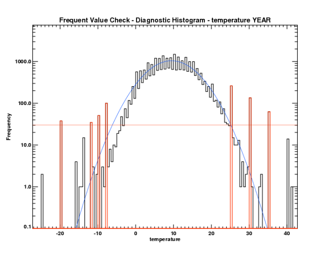
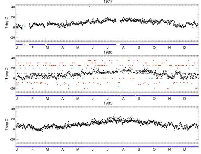
Abbildung 4: Frequent value check (test 4) for station 037930-99999, Anvil Green, Kent, UK (51.22^∘ N, 1.000^∘ E, 140 m), showing temperature. Top: Histogram with logarithmic y-axis for entire station record showing the bins which have been identified as being likely frequent values. Bottom: red points show values removed by this test and blue points by other tests for the years 1977, 1980 and 1983. The panel below each year indicates which station the observations come from in the case of a composite (not relevant here but is relevant in other station plots so included in all).

For each potential station match set, in addition to the hierarchical scoring system value (Table 1), were considered graphically the following quantities: 00:00 UTC temperature anomalies from the ISD-lite database (http://www.ncdc.noaa.gov/oa/climate/isd/index.php) using anomalies relative to the mean of the entire set of candidate station records; the ISD-lite data count by month; and the daily distribution of observing times. This required in-depth manual input taking roughly a calendar month to complete resulting in 1504 likely composite sets assigned as matches (comprising 3353 unique station IDs, Fig. 1). Of these just over half are very obviously the same station. For example, data ceased from one identifier simultaneously with data commencing from the other where the data are clearly not substantially inhomogeneous across the break; or the different identifiers report at different synoptic hours, but all other details are the same. Other cases were less clear, in most cases because data overlap implied potentially distinct stations or discontinuities yielding larger uncertainties in assignment. Assigned sets were merged giving initial preference to longer record segments but allowing infilling of missing elements where records overlap from the shorter segment records to maximise record completeness. This matching of stations was carried out on an earlier extraction of the ISD dataset spanning 1973 to 2007. The final dataset is based on an extraction from the ISD of data spanning 1973 to end-2011, and the station assignments have been carried over with no reanalysis.

There may well be assigned composites that should be separate stations, especially in densely sampled regions of the globe. If the merge were being done for the raw ISD archive that constitutes the baseline synoptic dataset held in the designated WMO World Data Centre, then far more meticulous analysis would be required. For this value added product a few false station merges can be tolerated and later amended/removed if detected. The station IDs that were combined to form a single record are noted in the metadata of the final output file where appropriate. A list of the identifiers of the 943 stations in the final dataset, which are assigned composites as well as their component station IDs, can be found on the HadISD website.

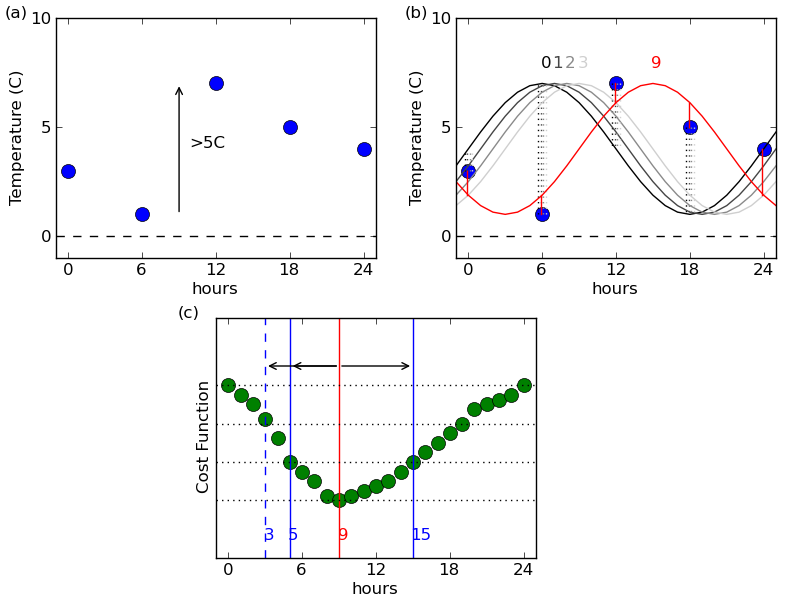
Abbildung 5: Schematic for the diurnal cycle check. (a) An example time series for a given day. There are observations in more than 3 quartiles of the day and the diurnal range is more than 5 ^∘C so the test will run. (b) A sine curve is fitted to the day observations. In this schematic case, the best fit that occurs has a 9-h shift. The cost function used to calculate the best fit is indicated by the dotted vertical lines. (c) The cost function distribution for each of the possible 24 offsets of the sine curve for this day. The terciles of the distribution are shown by horizontal black dotted lines. Where the cost function values enter the second tercile determines the uncertainty (vertical blue lines). The larger of the two differences (in this case 9 to 15 = 6 h) is chosen as the uncertainty. So if the climatological value is between 3 and 15 h, then this day does not have an anomalous diurnal cycle phase.

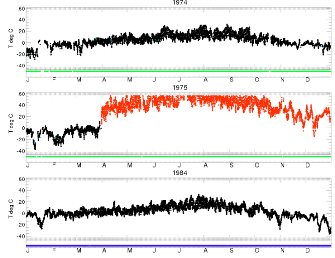
Abbildung 6: Distributional gap check (test 6) example for composite station 714740-99999, Clinton, BC, Canada (51.15^∘ N, 121.50^∘ W, 1057 m), showing temperature for the years 1974, 1975 and 1984. Red points show values removed by this test and blue points by other tests (none for the years shown). The panel below each year shows whether the data in the composited station come from the named station (blue) or a matched station (green). There is no change in source station within 1975, and so the compositing has not caused the clear offset observed therein, but the source station has changed for 1984 compared to the other two years.

2 Selection and retrieval of an initial set of stations

The ISD consists of a large number of stations, some of which have reported only rarely. Of the 30 000 stations, about 2/3 have observations for 30 yr or fewer and several thousand have small total file sizes, corresponding to few observations. However, almost 2000 stations have long records extending 60 or more years between 1901 and end-2011. Most of these have large total file sizes indicating quasi-continuous records, rather than only a few observations per year. To simplify selection, only stations that may plausibly have records suitable for climate applications were considered, using two key requirements: length of record and reporting frequency. The latter is important for characterisation of extremes, as too infrequent observing will greatly reduce the potential to capture both truly extreme events and the diurnal cycle characteristics. A degree of pre-screening was therefore deemed necessary prior to application of QC tests to winnow out those records that would be grossly inappropriate for climate studies.

To maximise spatial coverage, network distributions for four climatology periods (1976–2005, 1981–2000, 1986–2005 and 1991–2000) and four different average time steps between consecutive reports (hourly, 3-hourly, 6-hourly, 12-hourly) were compared. For a station to qualify for a climatology period, at least half of the years within the climatology period must have a corresponding data file regardless of its size. No attempt was made at this very initial screening stage to ensure these are well distributed within the climatological period. To assign the reporting frequency, (up to) the first 250 observations of each annual file were used to work out the average interval between consecutive observations. With hourly frequency, stipulation coverage collapses to essentially NW Europe and North America (Fig. 2). Three-hourly frequency yields a much more globally complete distribution. There is little additional coverage or station density derived by further coarsening to 6- (not shown) or 12-hourly except in parts of Australia, South America and the Pacific. Sensitivity to choice of climatology period is much smaller (not shown), so a 1976–2005 climatology period and a 3-hourly reporting frequency were chosen as a minimum requirement. This selection resulted in 6187 stations selected for further analysis.

Tabelle 2: Variables extracted from the ISD database and converted to netCDF for subsequent potential analysis. The second column indicates whether the value is an instantaneous measure or a time-averaged quantity. The third column shows the subset that we quality controlled and the fourth column the set included within the final files which includes some non-quality controlled variables.

	Instantaneous (I)	Subse-	Output
	or past period (P)	quent	in final
Variable	measurement	QC	dataset
Temperature	I	Y	Y
Dewpoint	I	Y	Y
SLP	I	Y	Y
Total cloud cover	I	Y	Y
High cloud cover	I	Y	Y
Medium cloud cover	I	Y	Y
Low cloud cover	I	Y	Y
Cloud base	I	N	Y
Wind speed	I	Y	Y
Wind direction	I	Y	Y
Present significant weather	I	N	N
Past significant weather #1	P	N	Y
Past significant weather #2	P	N	N
Precipitation report #1	P	N	Y
Precipitation report #2	P	N	N
Precipitation report #3	P	N	N
Precipitation report #4	P	N	N
Extreme temperature report #1	P	N	N
Extreme temperature report #2	P	N	N
Sunshine duration	P	N	N

ISD raw data files are (potentially) very large ASCII flat files – one per station per year. The stations data were converted to hourly resolution netCDF files for a subset of the variables including both WMO-designated mandatory and optional reporting parameters. Details of all variables retrieved and those considered further in the current quality control suite are given in Table 2. There are some stations which for part of the analysed period report at sub-hourly frequencies. As both temperature and dewpoint temperature are required to be measured simultaneously for any study on humidity to be reliably carried out, reports that have both temperature and dewpoint temperature observations are favoured (under the assumption that the readings were taken at close proximity in space and time) over those reports that have one or the other (but not both), even if the reports with both observations are further from the full hour. In cases where observations only have temperature or dewpoint temperature (and never both), then those with temperature are favoured, even if these are further from the full hour (00 min). All variables in a single HadISD hourly time step always derive from a single ISD time step, with no blending between the various within-hour reports. However the HadISD times are always converted to the nearest whole hour. To minimise data storage the time axis is collapsed in the netCDF files so that only time steps with observations are retained.

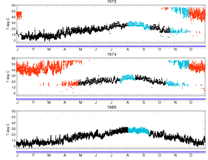
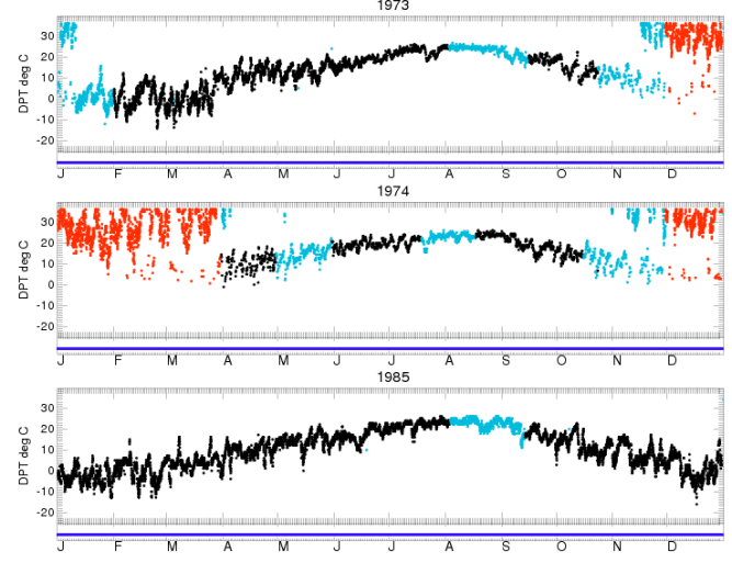
Abbildung 7: Distributional gap check (test 6) example when comparing all of a given calendar month in the dataset for composite station 476960-43323, Yokosuka, Japan (35.58^∘ N, 139.667^∘ E, 530 m), for (top) temperature and (middle) dewpoint temperature for the years 1973, 1974 and 1985. Red points show values removed by this test and blue points by other tests (in this case, mainly the diurnal cycle check). The problem for this station affects both variables, but the tests are applied separately. There is no change in source station in any of the years, and so compositing has not caused the bad data quality of this station.

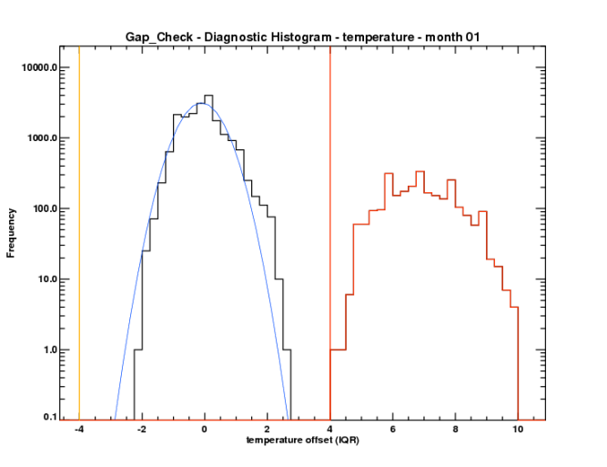
Abbildung 8: Distribution of the observations from all Januaries in the station record for composite station 476960-43323, Yokosuka, Japan (35.58^∘ N, 139.667^∘ E, 530 m). The population highlighted in red is removed by the distributional gap check (test 6), as shown in Fig. 7. Note logarithmic y-axis.

3 Quality control steps and analysis

An individual hourly station record with full temporal sampling from 1973 to 2011 could contain in excess of 340 000 observations and there are $>6$ 000 candidate stations. Hence, a fully automated quality-control procedure was essential. A similar approach to that of GHCND (Durre et al., 2010) was taken. Intra-station tests were initially trained against a single (UK) case-study station series with bad data deliberately introduced to ensure that the tests, at least to first order, behaved as expected. Both intra- and inter-station tests were then further designed, developed and validated based upon expert judgment and analysis using a set of 76 stations from across the globe (listed on the HadISD website). This set included both stations with proportionally large data removals in early versions of the tests and GCOS (Global Climate Observing System) Surface Network stations known to be highly equipped and well staffed so that major problems are unlikely. The test software suite took a number of iterations to obtain a satisfactorily small expert judgement false positive rate (type I error rate) and, on subjective assessment, a clean dataset for these stations. In addition, geographical maps of detection rates were viewed for each test and in total to ensure that rejection rates did not appear to have a real physical basis for any given test or variable. Deeper validation on UK stations (IDs beginning 03) was carried out using the well-documented 2003 heat wave and storms of 1987 and 1990. This resulted in a further round of refining, resulting in the tests as presented below.

Wherever distributional assumptions were made, an indicator that is robust to outliers was required. Pervasive data issues can lead to an unduly large standard deviation ($\sigma$) being calculated which results in the tests being too conservative. So, the inter-quartile range (IQR) or the median absolute deviation (MAD) was used instead; these sample solely the (presumably reasonable) core portion of the distribution. The IQR samples 50 per cent of the population, whereas $\pm 1$$\sigma$ encapsulates 68 per cent of the population for a truly normal distribution. One IQR is 1.35$\sigma$, and one MAD is 0.67$\sigma$ if the underlying data are truly normally distributed.

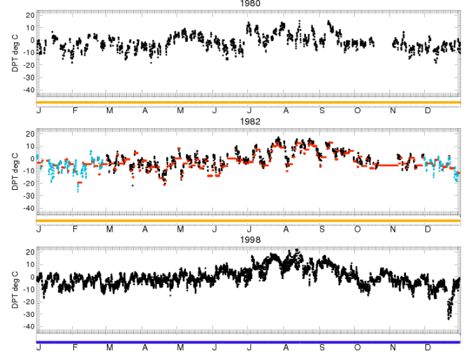
Abbildung 9: Repeated streaks/unusual streak frequency check (test 8) example for composite station 724797-23176 (Milford, UT, USA; 38.44^∘ N, 112.038^∘ W, 1534 m), for dewpoint temperature in 1982, illustrating frequent short streaks. Red points show values removed by this test and blue points by other tests. The panel below each year shows whether the data in the composited station come from the named station (blue) or a matched station (orange). There is no change in source station in 1982, and so the compositing has not caused the streaks observed in 1982, but a different station is used in 1998 compared to the other two years.

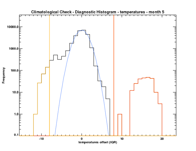
Abbildung 10: Climatological outlier check (test 9) for 040180-16201 (Keflavik, Iceland, 63.97^∘ N, 22.6^∘ W, 50 m) for temperature showing the distribution for May. Note logarithmic y-axis. The threshold values are shown by the vertical lines. The right-hand side shows the flagged values which occur further from the centre of the distribution than the gap and the threshold value. The left-hand side shows observations which have been tentatively flagged, as they are only further from the centre of the distribution than the threshold value. It is therefore not clear if the large tail is real or an artefact.

The Durre et al. (2010) method applies tests in a deliberate order, removing bad data progressively. Here, a slightly different approach is taken including a multi-level flagging system. All bad data have associated flags identifying the tests that they failed. Some tests result in instantaneous data removal (latitude-longitude and station duplicate checks), whereas most just flag the data. Flagged, but retained, data are not used for any further derivations of test thresholds. However, all retained data undergo each test such that an individual observation may receive multiple flags. Furthermore, some of the tests outlined in the next section set tentative flags. These values can be reinstated using comparisons with neighbouring stations in a later test, which reduces the chances of removing true local or regional extremes. The tests are conducted in a specified order such that large chunks of bad data are removed from the test threshold derivations first and so the tests become progressively more sensitive. After an initial latitude-longitude check (which removed one station) and a duplicate station check, intra-station tests are applied to the station in isolation, followed by inter-station neighbour comparisons. A subset of the intra-station tests is then re-run, followed by the inter-station checks again and then a final clean-up (Fig. 3).

3.1 QC tests

3.1.1 Test 1: inter-station duplicate check

It is possible that two unique station identifiers actually contain identical data. This may be simple data management error or an artefact of dummy station files intended for temporary data storage. To detect these, each station’s temperature time series is compared iteratively with that of every other station. To account for reporting time ($t$) issues, the series are offset by 1 h steps between $t-11$ and $t+11$ h. Series with $>1000$ coincident non-missing data points, of which over 25 per cent are flagged as exact duplicates, are listed for further consideration. This computer-intensive check resulted in 280 stations being put forward for manual scrutiny.

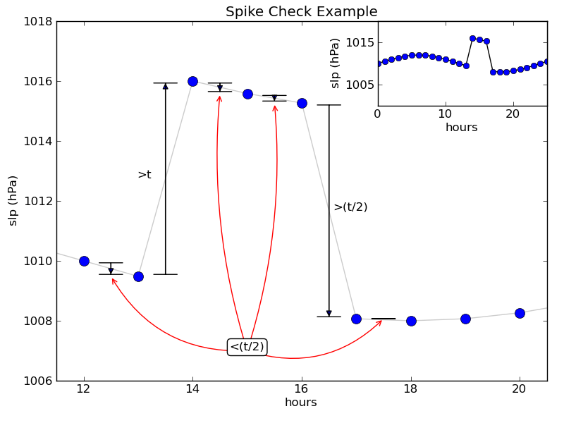
Abbildung 11: Spike check (test 10) schematic, showing the requirements on the first differences inside and outside of a multi-point spike. The inset shows the spike of three observations clearly above the rest of the time series. The first difference value leading into the spike has to be greater than the threshold value, $t$, and the first difference value coming out of the spike has to be of the opposite direction and at least half the threshold value ($t/2$). The differences outside and inside the spike (as pointed to by the red arrows) have to be less than half the threshold value.

All duplicate pairs and groups were then manually assessed using the match statistics, reporting frequencies, separation distance and time series of the stations involved. If a station pair had exact matches on $\geq 70$ per cent of potential occasions, then the shortest station of the pair was removed. This results in a further loss of stations. As this test is searching for duplicates after the merging of composite stations (Sect. 2), any stations found by this test did not previously meet the requirements for stations to be merged, but still have significant periods where the observations are duplicated. Therefore the removal of data is the safest course of action. Stations that appeared in the potential duplicates list twice or more were also removed. A further subjective decision was taken to remove any stations having a very patchy or obscure time series, for example with very high variance. This set of checks removed a total of 83 stations (Fig. 1), leaving 6103 to go forward into the rest of the QC procedure.

3.1.2 Test 2: duplicate months check

Given day-to-day weather, an exact match of synoptic data for a month with any other month in that station is highly unlikely. This test checks for exact replicas of whole months of temperature data where at least 20 observations are present. Each month is pattern-matched for data presence with all other months, and any months with exact duplicates for each matched value are flagged. As it cannot be known a priori which month is correct, both are flagged. Although the test was successful at detecting deliberately engineered duplication in a case study station, no occurrences of such errors were found within the real data. The test was retained for completeness and also because such an error may occur in future updates of HadISD.

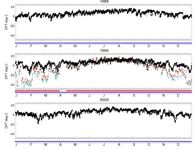
Abbildung 12: Spike check (test 10) for composite station 718936-99999 (49.95^∘ N, 125.267^∘ W, 106 m, Campbell River, BC, Canada), for dewpoint temperature showing the removal of a ghost station. Red points show values removed by this test and blue points by other tests. The panel below each year shows whether the data in the composited station come from the named station (blue) or a matched station (red). In 1988 and 2006 a single station is used for the data, but in 1996 there is clearly a blend between two stations (718936-99999 and 712050-99999). In this case the compositing has caused the ghosting; however, both these stations are labelled in the ISD history file as Campbell River, with identical latitudes and longitudes. An earlier period of merger between these two stations did not lead to any ghosting effects.

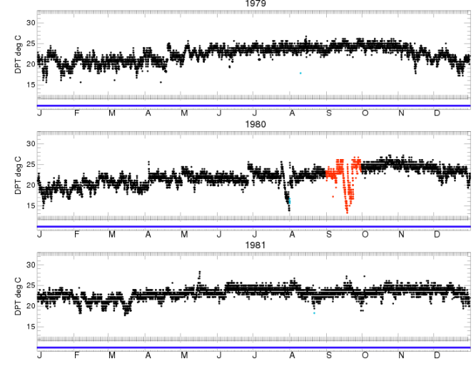
Abbildung 13: Unusual variance check (test 13) for (top) 912180-99999 (13.57^∘ N, 144.917^∘ E, 162 m, Andersen Air Force Base, Guam) for dewpoint temperature and (bottom) 133530-99999 (43.82^∘ N, 18.33^∘ E, 511 m, Sarajevo, Bosnia-Herzegovina) for temperature. Red points show values removed by this test and blue points by other tests (none for the years and variables shown).

3.1.3 Test 3: odd cluster check

A number of time series exhibit isolated clusters of data. An instrument that reports sporadically is of questionable scientific value. Furthermore, with little or no surrounding data it is much more difficult to determine whether individual observations are valid. Hence, any short clusters of up to 6 h within a 24 h period separated by 48 h or longer from all other data are flagged. This applies to temperature, dewpoint temperature and sea-level pressure elements individually. These flags can be undone if the neighbouring stations have concurrent, unflagged observations whose range encompasses the observations in question (see Sect. 3.1.14).

3.1.4 Test 4: frequent value check

The problem of frequent values found in Durre et al. (2010) also extends to synoptic data. Some stations contain far more observations of a given value than would be reasonably expected. This could be the use of zero to signify missing data, or the occurrence of some other local data-issue identifier that has been mistakenly ingested into the database as a true value. This test identifies suspect values using the entire record and then scans for each value on a year-by-year basis to flag only if they are a problem within that year.

This test is also run seasonally (JF + D, MAM, JJA, SON), using a similar approach as above. Each set of three months is scanned over the entire record to identify problem values (e.g. all MAMs over the entire record), but flags applied on an annual basis using just the three months on their own (e.g. each MAM individually, scanning for values highlighted in the previous step). As indicated by JF + D, the January and February are combined with the following December (from the same calendar year) to create a season, rather than working with the December from the previous calendar year. Performing a seasonal version, although having fewer observations to work with, is more powerful because the seasonal shift in the distribution of the temperatures and dewpoints can reveal previously hidden frequent values.

For the filtered (where previously flagged observations are not included) temperature, dewpoint and sea-level pressure data, histograms are created with 0.5 or 1.0 ^∘C or hPa increments (depending on the reporting accuracy of the measurement) and each histogram bin compared to the three on either side. If this bin contains more than half of the total population of the seven bins combined and also more than 30 observations over the station record (20 for the seasonal scan), then the histogram bin interval is highlighted for further investigation (Fig. 4). The minimum number limit was imposed to avoid removing true tails of the distribution.

Abbildung 14: Nearest neighbour data check (test 14) for 912180-99999 (13.57^∘ N, 144.917^∘ E, 162 m, Andersen Air Force Base, Guam) for sea-level pressure. Red points show values removed by this test (none for the years shown) and blue points by other tests. The spikes for the hurricanes in 1976 and 1977 are kept in the dataset. February 1976 is removed by the variance check – this February has higher variance than expected when compared to all other Februaries for this station.

After this identification stage, the unfiltered distribution is studied on a yearly basis. If the highlighted bins are prominent (contain $>50$ per cent of the observations of all seven bins and more than 20 observations in the year, or $90$ per cent of the observations of all seven bins and more than 10 observations in the year) in any year, then they are flagged (the bin sizes are reduced to 15 and 10 respectively for the seasonal scan). This two-stage process was designed to avoid removing too many valid observations (type II errors). However, even with this method, by flagging all values within a bin it is likely that some real data are flagged if the values are sufficiently close to the mean of the overall data distribution. Also, frequent values that are pervasive for only a few years out of a longer record and are close to the distribution peak may not be identified with this method (type I errors). However, alternative solutions were found to be too computationally inefficient. Station 037930-99999 (Anvil Green, Kent, UK) shows severe problems from frequent values in the temperature data for 1980 (Fig. 4). Temperature and dewpoint flags are synergistically applied, i.e. temperature flags are applied to both temperature and dewpoint data, and vice versa.

3.1.5 Test 5: diurnal cycle check

All ISD data are archived as UTC; conversion has generally taken place from local time at some point during recording, reporting and archiving the data. Errors could introduce large biases into the data for some applications that consider changes in the diurnal characteristics. The test is only applied to stations at latitudes below 60^∘ N/S as above these latitudes the diurnal cycle in temperature can be weak or absent, and obvious robust geographical patterns across political borders were apparent in the test failure rates when it was applied in these regions.

This test is run on temperature only as this variable has the most robust diurnal cycle, but it flags data for all variables. Firstly, a diurnal cycle is calculated for each day with at least four observations spread across at least three quartiles of the day (see Fig. 5). This is done by fitting a sine curve with amplitude equal to half the spread of reported temperatures on that day. The phase of the sine curve is determined to the nearest hour by minimising a cost function, namely the mean squared deviations of the observations from the curve (see Fig. 5). The climatologically expected phase for a given calendar month is that with which the largest number of individual days phases agrees. If a day’s temperature range is less than 5 ^∘C, no attempt is made to determine the diurnal cycle for that day.

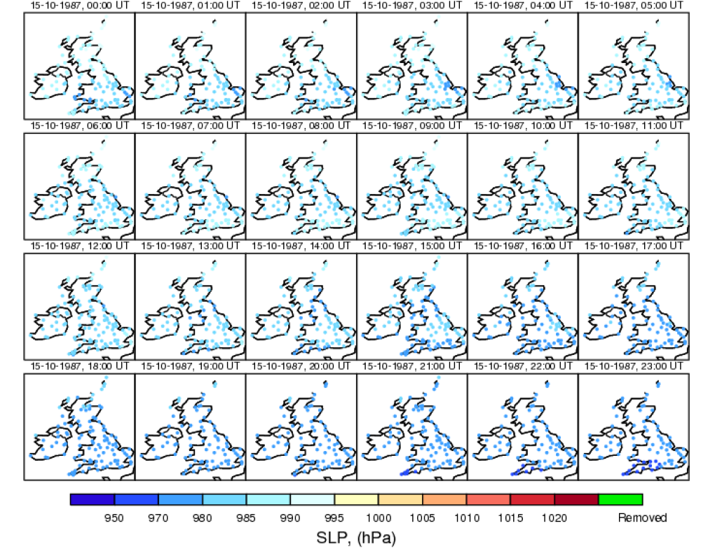
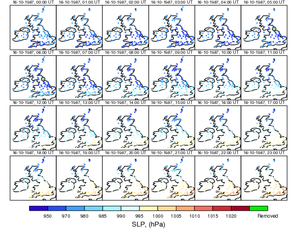
Abbildung 15: Passage of low pressure core over the British Isles during the night of 15–16 October 1987. Green points (highlighted by circles) are stations where the observation for that hour has been removed. There are two, at 05:00 and 06:00 UTC, on 16 October 1987 in the north-east of England. These flagged observations are investigated in Fig. 16.

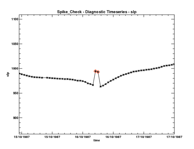
Abbildung 16: Sea level pressure data from station 032450-99999 (Newcastle Weather Centre, 54.967^∘ N, $-$1.617^∘ W, 47 m) during mid-October 1987. The two observations that have triggered the spike check are clearly visible and are distinct from the rest of the data. Given their values (994.6 and 993.1 hPa), the two flagged observations are clearly separate from their adjacent ones (966.4 and 963.3 hPa). It is possible that a keying error in the SYNOP report led to 946 and 931 being reported, rather than 646 and 631. However, we make no attempt in this dataset to rescue flagged values.

It is then assessed whether a given day’s fitted phase matches the expected phase within an uncertainty estimate. This uncertainty estimate is the larger of the number of hours by which the day’s phase must be advanced or retarded for the cost function to cross into the middle tercile of its distribution over all 24 possible phase-hours for that day. The uncertainty is assigned as symmetric (see Fig. 5). Any periods $>30$ days where the diurnal cycle deviates from the expected phase by more than this uncertainty, without three consecutive good or missing days or six consecutive days consisting of a mix of only good or missing values, are deemed dubious and the entire period of data (including all non-temperature elements) is flagged.

Small deviations, such as daylight saving time (DST) reporting hour changes, are not detected by this test. This type of problem has been found for a number of Australian stations where during DST the local time of observing remains constant, resulting in changes in the common GMT reporting hours across the year. Such changes in reporting frequency and also the hours on which the reports are taken are noted in the metadata of the netCDF file.

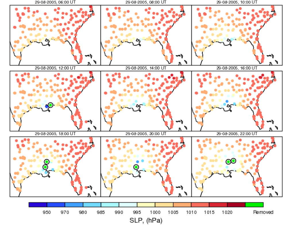
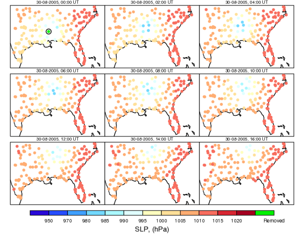
Abbildung 17: Passage of low pressure core of Hurricane Katrina during its landfall in 2005. Every second hour is shown. Green points are observations which have been removed, in this case by the neighbour outlier check (see test 14).

3.1.6 Test 6: distributional gap check

Portions of a time series may be erroneous, perhaps originating from station ID issues, recording or reporting errors, or instrument malfunction. To capture these, monthly medians $M_{ij}$ are created from the filtered data for calendar month $i$ in year $j$. All monthly medians are converted to anomalies $A_{ij}\equiv M_{ij}-M_{i}$ from the calendar monthly median $M_{i}$ and standardised by the calendar month inter-quartile range IQR_i (inflated to 4 ^∘C or hPa for those months with very small IQR_i) to account for any seasonal cycle in variance. The station’s series of standardised anomalies $S_{ij}A_{ij}/\textrm{IQR}_{i}$ is then ranked, and the median, $\acute{S}$, obtained.

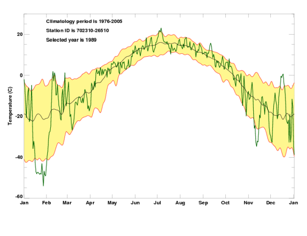
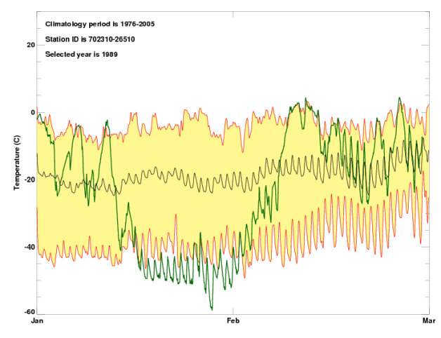
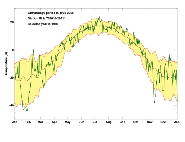
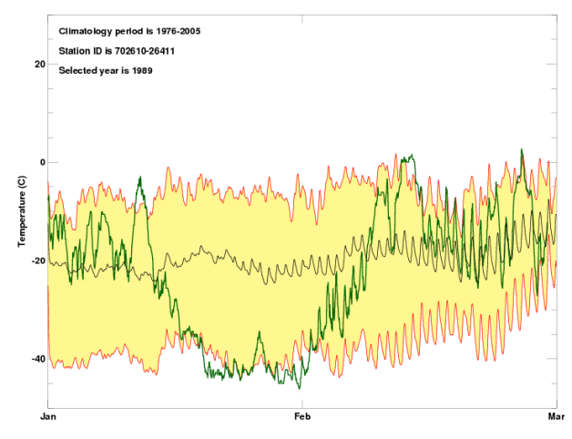
Abbildung 18: Left: Alaskan daily mean temperature in 1989 (green curve) shown against the climatological daily average temperature (black line) and the 5th and 95th percentile region, red curves and yellow shading. The cold spell in late January is clearly visible. Right: similar plots, but showing the sub-daily resolution data for a two month period starting in January 1989. The climatology, 5th and 95th percentile lines have been smoothed using an 11-point binomial filter in all four plots. Top: McGrath (702310-99999, 62.95^∘ N, 155.60^∘ W, 103 m), bottom: Fairbanks (702610-26411, 64.82^∘ N, 147.86^∘ W, 138 m).

Firstly, all observations in any month and year with $S_{ij}$ outside the range $\pm 5$ (in units of the IQR_i) from $\acute{S}$ are flagged, to remove gross outliers. Then, proceeding outwards from $\acute{S}$, pairs of $S_{ij}$ above and below ($S_{iu}$, $S_{iv}$) it are compared in a step-wise fashion. Flagging is triggered if one anomaly $S_{iu}$ is at least twice the other $S_{iv}$ and both are at least 1.5IQR_i from $\acute{S}$. All observations are flagged for the months for which $S_{ij}$ exceeds $S_{iu}$ and has the same sign. This flags one entire tail of the distribution. This test should identify stations that have a gap in the data distribution, which is unrealistic. Later checks should find any issues existing in the remaining tail. Station 714740-99999 (Clinton, BC, Canada, an assigned composite) shows an example of the effectiveness of this test at highlighting a significantly outlying period in temperature between 1975 and 1976 (Fig. 6).

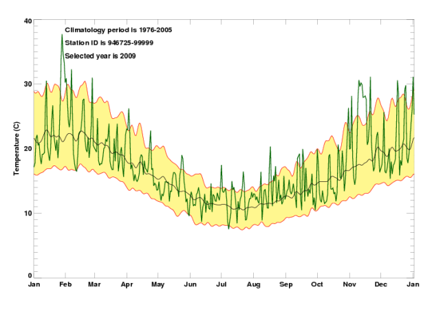
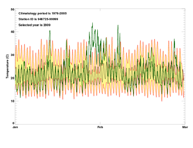
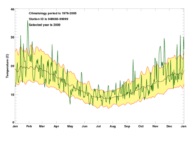
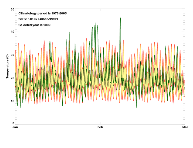
Abbildung 19: Left: daily mean temperature in southern Australia in 2009 (green curve) with climatological average (black line) and 5th and 95th percentiles (red lines and yellow shading). The exceptionally high temperatures in late January/early February and mid-November can clearly be seen. Right: similar plots showing the full sub-daily resolution data for a two month period starting in January 2009. The climatology, 5th and 95th percentile lines have been smoothed using an 11-point binomial filter in all four plots. Top: Adelaide (946725-99999, 34.93^∘ S, 138.53^∘ E, 4 m), bottom: Melbourne (948660-99999, 37.67^∘ S, 144.85^∘ E, 119 m).

An extension of this test compares all the observations for a given calendar month over all years to look for outliers or secondary populations. A histogram is created from all observations within a calendar month. To characterise the width of the distribution for this month, a Gaussian curve is fitted. The positions where this expected distribution crosses the $y=0.1$ line are noted, and rounded outwards to the next integer-plus-one to create a threshold value. From the centre outwards, the histogram is scanned for gaps, i.e. bins which have a value of zero. When a gap is found, and it is large enough (at least twice the bin width), then any bins beyond the end of the gap, which are also beyond the threshold value, are flagged.

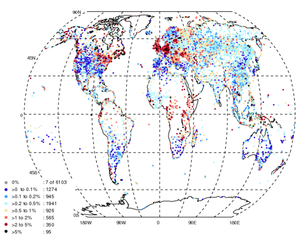
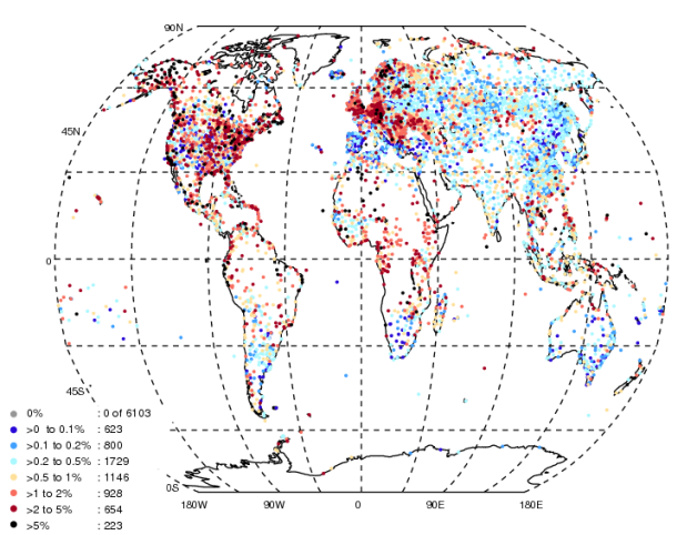
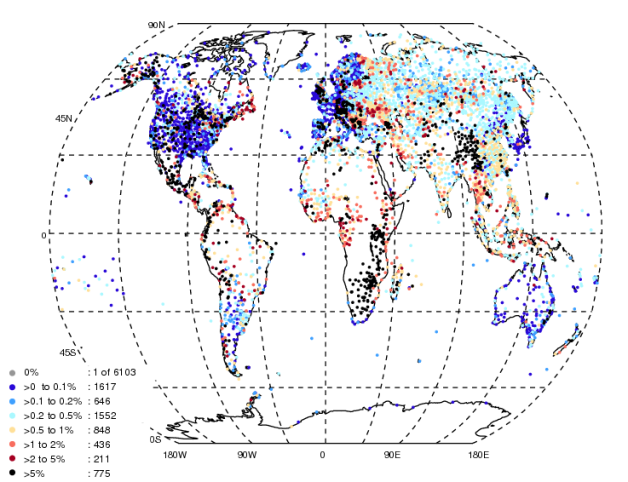
Abbildung 20: Rejection rates by variable for each station. Top panel: temperature, Middle panel: dewpoint temperature, and Lower Panel: sea-level pressure. Different rejection rates are shown by different colours, and the key in each panel provides the total number of stations in each band.

Although a Gaussian fit may not be optimal or appropriate, it will account for the spread of the majority of observations for each station, and the contiguous portion of the distribution will be retained. For Station 476960-43323 (Yokosuka, Japan, an assigned composite) this part of the test flags a number of observations. In fact, during the winter all temperature measurements below 0 ^∘C appear to be measured in Fahrenheit (see Fig. 7). In months that have a mixture of above and below 0 ^∘C data (possibly Celsius and Fahrenheit data), the monthly median may not show a large anomaly, so this extension is needed to capture the bad data. Figure 7 shows that the two clusters of red points in January and October 1973 are captured by this portion of the test. By comparing the observations for a given calendar month over all years, the difference between the two populations is clear (see bottom panel in Fig. 8). If there are two, approximately equally sized distributions in the station record, then this test will not be able to choose between them.

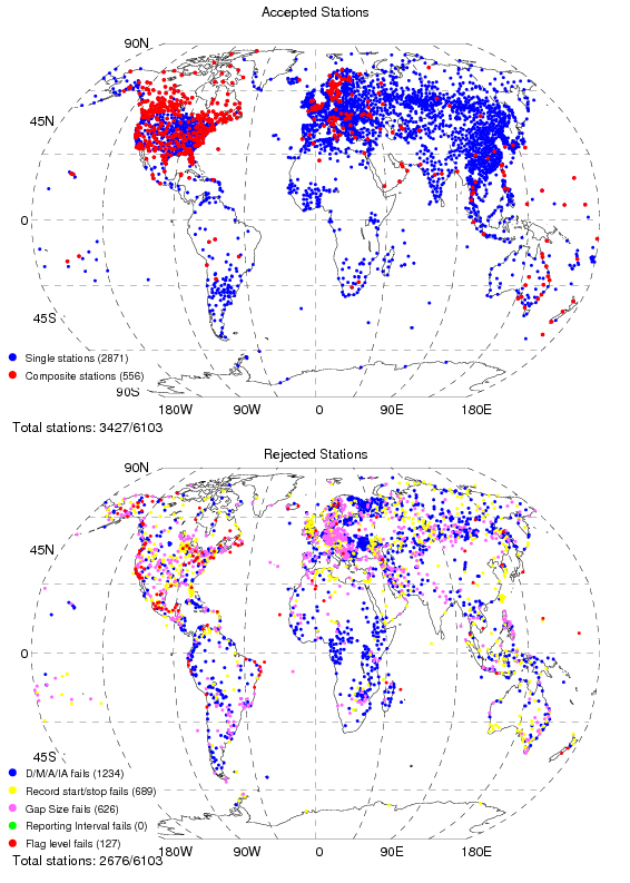
Abbildung 21: The results of the final filtering to select climate quality stations. Top: the selected stations that pass the filtering, with red for composite stations (556/3427). Bottom: the rejected stations. Of these, 1234/2676 fail to meet the daily, monthly, annual or interannual requirements (D/M/A/IA); 689/2676 begin after 1980 or end before 2000; 626/2676 have a gap exceeding two years after the daily, monthly and annual completeness criteria have been applied; and 127 fail because one of the three main variables has a high proportion of flags.

To prevent the low pressure extremes associated with tropical cyclones being excessively flagged, any low SLP observation identified by this second part of the test is only tentatively flagged. Simultaneous wind speed observations, if present, are used to identify any storms present, in which case low SLP anomalies are likely to be true. If the simultaneous wind speed observations exceed the median wind speed for that calendar month by 4.5 MADs, then storminess is assumed and the SLP flags are unset. If there are no wind data present, the neighbouring stations can be used to unset these tentative flags in test 14. The tentative flags are only used for SLP observations in this test.

3.1.7 Test 7: known records check

Absolute limits are assigned based on recognised and documented world and regional records (Table 3). All hourly observations outside these limits are flagged. If temperature observations exceed a record, the dewpoints are synergistically flagged. Recent analyses of the record Libyan temperature have resulted in a change to the global and African temperature record (Fadli et al., 2012). Any observations that would be flagged using the new value but not by the old are likely to have been flagged by another test. This only affects African observations, and those not assigned to the WMO regions outlined in Table 3. The value used by this test will be updated in a future release of HadISD.

Abbildung 22: The median diurnal temperature ranges recorded by each station (using the selected 3427 stations) for each of the four three-month seasons. Top-left for December-January-February, top-right for March-April-May, bottom-left for June-July-August and bottom-right for September-October-November.

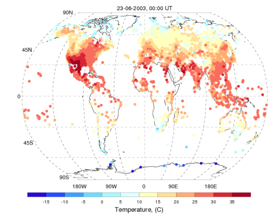
Abbildung 23: The temperature for each station on the 23 June 2003 at 00:00, 06:00, 12:00 and 18:00 UT using all 6103 stations.

Tabelle 3: Extreme limits for observed variables gained from http://wmo.asu.edu (the official WMO climate extremes repository) and the GHCND tests. Dewpoint minima are estimates based upon the record temperature minimum for each region. First element in each cell is the minimum and the second the maximum legal value. Regions follow WMO regional definitions and are given at: http://weather.noaa.gov/tg/site.shtml. Global values are used for any station where the assigned WMO identifier is missing or does not fall within the region categorization. Wind speed and sea-level pressure records are not currently documented regionally so global values are used throughout. We note that the value for the African and global maximum temperature has changed (Fadli et al., 2012). This will be updated in a future version of HadISD.

Region	Temperature			Dewpoint Temperature			Wind speed			Sea-level pressure
	(∘C)			(∘C)			(m s-1)			(hPa)
	max	min		max	min		max	min		max	min
Global	$-$89.2	57.8		$-$100.0	57.8		0.0	113.3		870	1083.3
Africa	$-$23.0	57.8		$-$50.0	57.8		–	–		–	–
Asia	$-$67.8	53.9		$-$100.0	53.9		–	–		–	–
S. America	$-$32.8	48.9		$-$60.0	48.9		–	–		–	–
N. America	$-$63.0	56.7		$-$100.0	56.7		–	–		–	–
Pacific	$-$23.0	50.7		$-$50.0	50.7		–	–		–	–
Europe	$-$58.1	48.0		$-$100.0	48.0		–	–		–	–
Antarctica	$-$89.2	15.0		$-$100.0	15.0		–	–		–	–

3.1.8 Test 8: repeated streaks/unusual spell frequency

This test searches for consecutive observation replication, same hour observation replication over, a number of days (either using a threshold of a certain number of observations, or for sparser records, a number of days during which all the observations have the same value) and also whole day replication for a streak of days. All three tests are conditional upon the typical reporting precision as coarser precision reporting (e.g. temperatures only to the nearest whole degree) will increase the chances of a streak arising by chance (Table 4). For wind speed, all values below 0.5 ms^-1 (or 1 ms^-1 for coarse recording resolution) are also discounted in the streak search given that this variable is not normally distributed and there could be long streaks of calm conditions.

Tabelle 4: Streak check criteria and their assigned sensitivity to typical within-station reporting resolution for each variable.

	Reporting	Straight repeat	Hour repeat	Day repeat
Variable	resolution	streak criteria	streak criteria	streak criteria
	1 ∘C	40 values of 14 days	25 days	10 days
Temperature	0.5 ∘C	30 values or 10 days	20 days	7 days
	0.1 ∘C	24 values or 7 days	15 days	5 days
	1 ∘C	80 values of 14 days	25 days	10 days
Dewpoint	0.5 ∘C	60 values or 10 days	20 days	7 days
	0.1 ∘C	48 values or 7 days	15 days	5 days
	1 hPa	120 values of 28 days	25 days	10 days
SLP	0.5 hPa	100 values or 21 days	20 days	7 days
	0.1 hPa	72 values or 14 days	15 days	5 days
	1 ms-1	40 values of 14 days	25 days	10 days
Wind speed	0.5 ms-1	30 values or 10 days	20 days	7 days
	0.1 ms-1	24 values or 7 days	15 days	5 days

During development of the test a number of station time series were found to exhibit an alarming frequency of streaks shorter than the assigned critical lengths in some years. An extra criterion was added to flag all streaks in a given year when consecutive value streaks of $>10$ elements occur with extraordinary frequency ($>5$ times the median annual frequency). Station 724797-23176 (Milford, UT, USA, an assigned composite) exhibits a propensity for streaks during 1981 and 1982 in the dewpoint temperature (Fig. 9), which is not seen in any other years or nearby stations.

3.1.9 Test 9: climatological outlier check

Individual gross outliers from the general station distribution are a common error in observational data caused by random recording, reporting, formatting or instrumental errors (Fiebrich and Crawford, 2009). This test uses individual observation deviations derived from the monthly mean climatology calculated for each hour of the day. These climatologies are calculated using observations that have been winsorised to remove the initial effects of outliers. The raw, un-winsorised observations are anomalised using these climatologies and standardised by the IQR for that month and hour. Values are subsequently low-pass filtered to remove any climate change signal that would cause overzealous removal at the ends of the time series. In an analogous way to the distributional gap check, a Gaussian is fitted to the histogram of these anomalies for each month, and a threshold value, rounded outwards, is set where this crosses the $y=0.1$ line. The distribution beyond this threshold value is scanned for a gap (equal to the bin width or more), and all values beyond any gap are flagged. Observations that fall between the critical threshold value and the gap or the critical threshold value and the end of the distribution are tentatively flagged, as they fall outside of the expected distribution (assuming it is Gaussian; see Fig. 10). These may be later reinstated on comparison with good data from neighbouring stations (see Sect. 3.1.14). A caveat to protect low-variance stations is added whereby the IQR cannot be less than 1.5 ^∘C. When applied to sea-level pressure, this test frequently flags storm signals, which are likely to be of high interest to many users, and so this test is not applied to the pressure data.

As for the distributional gap check, the Gaussian may not be the best fit or even appropriate for the distribution, but by fitting to the observed distribution, the spread of the majority of the observations for the station is accounted for, and searching for a gap means that the contiguous portion of distribution is retained.

3.1.10 Test 10: spike check

Unlike the operational ISD product, which uses a fixed value for all stations (Lott et al., 2001), this test uses the filtered station time series to decide what constitutes a “spike”, given the statistics of the series. This should avoid over zealous flagging of data in high variance locations but at a potential cost for stations where false data spikes are truly pervasive. A first difference series is created from the filtered data for each time step (hourly, 2-hourly, 3-hourly) where data exist within the past three hours. These differences for each month over all years are then ranked and the IQR calculated. Critical values of 6 times the rounded-up IQR are calculated for one-, two- and three-hourly differences on a monthly basis to account for large seasonal cycles in some regions. There is a caveat that no critical value is smaller than 1 ^∘C or hPa (conceivable in some regions but below the typically expected reported resolution). Also hourly critical values are compared with two hourly critical values to ensure that hourly values are not less than 66 per cent of two hourly values. Spikes of up to three sequential observations in the unfiltered data are defined by satisfying the following criteria. The first difference change into the spike has to exceed the threshold and then have a change out of the spike of the opposite sign and at least half the critical amplitude. The first differences just outside of the spike have to be under the critical values, and those within a multi-observation spike have to be under half the critical value (see Fig. 11 highlighting the various thresholds). These checks ensure that noisy high variance stations are not overly flagged by this test. Observations at the beginning or end of a contiguous set are also checked for spikes by comparing against the median of the subsequent or previous 10 observations. Spike check is particularly efficient at flagging an apparently duplicate period of record for station 718936-99999 (Campbell River, Canada, an assigned composite station), together with the climatological check (Fig. 12).

3.1.11 Test 11: temperature and dewpoint temperature cross-check

Following (Willett et al., 2008), this test is specific to humidity-related errors and searches for three different scenarios:

1. Supersaturation (dewpoint temperature $>$ temperature), although physically plausible especially in very cold and humid climates (Makkonen and Laakso, 2005), is highly unlikely in most regions. Furthermore, standard meteorological instruments are unreliable at measuring this accurately.

2. Wet-bulb reservoir drying (due to evaporation or freezing) is very common in all climates, especially in automated stations. It is evidenced by extended periods of temperature equal to dewpoint temperature (dewpoint depression of 0 ^∘C).

3. Cutoffs of dewpoint temperatures at temperature extremes. Systematic flagging of dewpoint temperatures when the simultaneous temperature exceeds a threshold (specific to individual National Meteorological Services’ recording methods) has been a common practice historically with radiosondes (Elliott, 1995; McCarthy et al., 2009). This has also been found in surface stations both for hot and cold extremes (Willett et al., 2008).

For supersaturation, only the dewpoint temperature is flagged if the dewpoint temperature exceeds the temperature. The temperature data may still be desirable for some users. However, if this occurs for 20 per cent or more of the data within a month, then the whole month is flagged. In fact, no values are flagged by this test and a later, independent check run at NCDC showed that there were no episodes of supersaturation in the raw ISD (Neal Lott, personal communication). However it is retained for completeness. For wet-bulb reservoir drying, all continuous streaks of absolute dewpoint depression $<0.25$ ^∘C are noted. The leeway of $\pm 0.25$ ^∘C allows for small systematic differences between the thermometers. If a streak is $>24$ h with $\geq$ four observations present, then all the observations of dewpoint temperature are flagged unless there are simultaneous precipitation or fog observations for more than one-third of the continuous streak. We use a cloud base measurement of $<1000$ feet to indicate fog as well as the present weather information. This attempts to avoid over zealous flagging in fog- or rain-prone regions (which would dry-bias the observations if many fog or rain events were removed). However, it is not perfect as not all stations include these variables. For cutoffs, all observations within a month are binned into 10 ^∘C temperature bins from $-$90 ^∘C to 70 ^∘C (a range that extends wider than recognised historically recorded global extremes). For any month where at least 50 per cent of temperatures within a bin do not have a simultaneous dewpoint temperature, all temperature and dewpoint data within the bin are flagged. Reporting frequencies of temperature and dewpoint are identified for the month, and removals are not applied where frequencies differ significantly between the variables. The cutoffs part of this test can flag good dewpoint data even if only a small portion of the month has problems, or if there are gaps in the dewpoint series that are not present in the temperature observations.

3.1.12 Test 12: cloud coverage logical checks

Synoptic cloud data are a priori a very difficult parameter to test for quality and homogeneity. Traditionally, cloud base height and coverage of each layer (low, mid, and high) in oktas were estimated by eye. Now cloud is observed in many countries primarily using a ceilometer which takes a single 180^∘ scan across the sky with a very narrow off-scan field-of-view. Depending on cloud type and cloud orientation, this could easily under- or over-estimate actual sky coverage. Worse, most ceilometers can only observe low or at best mid-level clouds. Here, a conservative approach has been taken where simple cross checking on cloud layer totals is used to infer basic data quality. This should flag the most glaring issues but does not guarantee a high quality database.

Six tests are applied to the data. If coverage at any level is given as 9 or 10, which officially mean sky obscured and partial obstruction respectively, that individual value is flagged. If total cloud cover is less than the sum of low, middle and high level cloud cover, then all are flagged. If low cloud is given as 8 oktas (full coverage) but middle or high level clouds have a value, then, as it is not immediately apparent which observations are at fault, the low, middle and/or high cloud cover values are flagged. If middle layer cloud is given as 8 oktas (full coverage) but high level clouds have a value, then, similarly, both the middle and high cloud cover value are flagged. If the cloud base height is given as 22 000, this means that the cloud base is unobservable (sky is clear). This value is then set to $-$10 for computational reasons. Finally, cloud coverage can only be from 0 to 8 oktas. Any value of total, low, middle layer or high cloud that is outside these bounds is flagged.

3.1.13 Test 13: unusual variance check

The variance check flags whole months of temperature, dewpoint temperature and sea-level pressure where the within month variance of the normalised anomalies (as described for climatological check) is sufficiently greater than the median variance over the full station series for that month based on winsorised data (Afifi and Azen, 1979). The variance is taken as the MAD of the normalised anomalies in each individual month with $\geq 120$ observations. Where there is sufficient representation of that calendar month within the time series (10 months each with $\geq 120$ observations), a median variance and IQR of the variances are calculated. Months that differ by more than 8 IQR (temperatures and dewpoints) or 6 IQR (sea-level pressures) from the station month median are flagged. This threshold is increased to 10 or 8 IQR respectively if there is a reduction in reporting frequency or resolution for the month relative to the majority of the time series.

Sea-level pressure is accorded special treatment to reduce the removal of storm signals (extreme low pressure). The first difference series is taken. Any month where the largest consecutive negative or positive streak in the difference series exceeds 10 data points is not considered for removal as this identifies a spike in the data that is progressive rather than transient. Where possible, the wind speed data are also included, and the median found for a given month over all years of data. The presence of a storm is determined from the wind speed data in combination with the sea-level pressure profile. When the wind speed climbs above 4.5 MADs from the median wind speed value for that month and if this peak is coincident with a minimum of the sea-level pressure ($\pm 24$ h), which is also more than 4.5 MADs from the median pressure for that month, then storminess is assumed. If these criteria are satisfied, then no flag is set. This test for storminess includes an additional test for unusually low SLP values, as initially this QC test only identifies periods of high variance. Figure 13, for station 912180-99999 (Andersen Air Force Base, Guam), illustrates how this check is flagging obviously dubious dewpoints that previous tests had failed to identify.

3.1.14 Test 14: nearest neighbour data checks

Recording, reporting or instrument error is unlikely to be replicated across networks. Such an error may not be detectable from the intra-station distribution, which is inherently quite noisy. However, it may stand out against simultaneous neighbour observations if the correlation decay distance (Briffa and Jones, 1993) is large compared to the actual distance between stations and therefore the noise in the difference series is comparatively low. This is usually true for temperature, dewpoint and pressure. However the check is less powerful for localised features such as convective precipitation or storms.

Tabelle 5: Summary of tests applied to the data.

Test	Applies to						Test failure	Notes
(Number)	T	Td	SLP	ws	wd	clouds	criteria
Intra-station
Duplicate months check (2)	X	X	X	X	X	X	Complete match to least temporally complete month’s record for T
Odd cluster check (3)	X	X	X	X	X		$\leq 6$ values in 24 h separated from any other data by $>48$ h	Wind direction removed using wind speed characteristics
Frequent values check (4)	X	X	X				Initially $>50$ % of all data in current 0.5 ∘C or hPa bin out of this and $\pm 3$ bins for all data to highlight, with $\geq 30$ in the bin. Then on yearly basis using highlighted bins with $>50$ % of data and $\geq 20$ observations in this and $\pm 3$ bins OR $>90$ % data and $\geq 10$ observations in this and $\pm 3$ bins. For seasons, the bin size thresholds are reduced to 20, 15 and 10 respectively.	Histogram approach for computational expediency. T and Td synergistically removed, if T is bad, then Td is removed and vice versa.
Diurnal cycle check (5)	X	X	X	X	X	X	30 days without 3 consecutive good fit/missing or 6 days mix of these to T diurnal cycle.
Distributional gap check (6)	X	X	X				Monthly median anomaly $>5$IQR from median. Monthly median anomaly at least twice the distance from the median as the other tail and $>1.5$ IQR. Data outside of the Gaussian distribution for each calendar month over all years, separated from the main population.	All months in tail with apparent gap in the distribution are removed beyond the assigned gap for the variable in question. Using the distribution for all calendar months, tentative flags set if further from mean than threshold value. To keep storms, low SLP observations are only tentatively
Known record check (7)	X	X	X	X			See Table 3	Td flagged if T flagged.
Repeated streaks/unusual spell frequency check (8)	X	X	X	X			See Table 4
Climatological outliers check (9)	X	X					Distribution of normalised (by IQR) anomalies investigated for outliers using same method as for distributional gap test.	To keep low variance stations, minimum IQR is 1.5 ∘C
Spike check (10)	X	X	X				Spikes of up to 3 consecutive points allowed. Critical value of 6IQR (minimum 1 ∘C or hPa) of first difference at start of spike, at least half as large and in opposite direction at end.	First differences outside and inside a spike have to be under the critical and half the critical values respectively
T and Td cross-check: Supersaturation (11)		X					Td $>$ T	Both variables removed, all data removed for a month if $>20$ % of data fails
T and Td cross-check: Wet bulb drying (11)		X					T $=$ Td $>24$ h and $>4$ observations unless rain / fog (low cloud base) reported for $>1/3$ of string	0.25 ∘C leeway allowed.
T and Td cross-check: Wet bulb cutoffs (11)		X					$>20$ % of T has no Td within a 10 ∘C T bin	Takes into account that Td at many stations reported less frequently than T.
Cloud coverage logical checks (12)						X	Simple logical criteria (see Sect. 3.1.12)
Unusual variance check (13)	X	X	X				Winsorised normalised (by IQR) anomalies exceeding 6 IQR after filtering	8 IQR if there is a change in reporting frequency or resolution. For SLP first difference series used to find spikes (storms). Wind speed also used to identify storms

Tabelle 5: Continued.

Test	Applies to						Test failure	Notes
(Number)	T	Td	SLP	ws	wd	clouds	criteria
Intra-station
Inter-station duplicate check (1)	X						$>1000$ valid points and $>25$ % exact match over $t-11$ to $t+11$ window, followed by manual assessment of identified series	Stations identified as duplicates removed in entirety.
Nearest neighbour data check (14)	X	X	X				$>2/3$ of station comparisons suggest the value is anomalous within the difference series at the 5 IQR level.	At least three and up to ten neighbours within 300 km and 500 m, with preference given to filling directional quadrants over distance in neighbour selection. Pressure has additional caveat to ensure against removal of severe storms.
Station clean-up (15)	X	X	X	X	X		$<20$ values per month or $>40$ % of values in a given month flagged for the variable	Results in removal of whole month for that variable

For each station, up to ten nearest neighbours (within 500 m elevation and 300 km distance) are identified. Where possible, all four quadrants (northeast, southeast, southwest and northwest) surrounding the station must be represented by at least two neighbours to prevent geographical biases arising in areas of substantial gradients such as frontal regions. Where there are less than three valid neighbours, the nearest neighbour check is not applied. In such cases the station ID is noted, and these stations can be found on the HadISD website. The station may be of questionable value in any subsequent homogenisation procedure that uses neighbour comparisons. A difference series is created for each candidate station minus neighbour pair. Any observation associated with a difference exceeding 5IQR of the whole difference series is flagged as potentially dubious. For each time step, if the ratio of dubious candidate-neighbour differences flagged to candidate-neighbour differences present exceeds 0.67 (2 in 3 comparisons yield a dubious value), and there are three or more neighbours present, then the candidate observation differs substantially from most of its neighbours and is flagged. Observations where there are fewer than three neighbours that have valid data are noted in the flag array.

For sea-level pressure in the tropics, this check would remove some negative spikes which are real storms as the low pressure core can be narrow. So, any candidate-neighbour pair with a distance greater than 100 km between is assessed. If 2/3 or more of the difference series flags (over the entire record) are negative (indicating that this site is liable to be affected by tropical storms), then only the positive differences are counted towards the potential neighbour outlier removals when all neighbours are combined. This succeeds in retaining many storm signals in the record. However, very large negative spikes in sea-level pressure (tropical storms) at coastal stations may still be prone to removal especially just after landfall in relatively station dense regions (see Sect. 4.1). Here, station distances may not be large enough to switch off the negative difference flags but distant enough to experience large differences as the storm passes. Isolated island stations are not as susceptible to this effect, as only the station in question will be within the low-pressure core and the switch off of negative difference flags will be activated. Station 912180-99999 (Anderson, Guam) in the western Tropical Pacific has many storm signals in the sea-level pressure (Fig. 14). It is important that these extremes are not removed.

Flags from the spike, gap (tentative low SLP flags only; see Sect. 3.1.6), climatological (tentative flags only; see Sect. 3.1.9), odd cluster and dewpoint depression tests (test numbers 3, 6, 9, 10 & 11) can be unset by the nearest neighbour data check. For the first four tests this occurs if there are three or more neighbouring stations that have simultaneous observations that have not been flagged. If the difference between the observation for the station in question and the median of the simultaneous neighbouring observations is less than the threshold value of 4.5 MADs, then the flag is removed. These criteria are to ensure that only observations that are likely to be good can have their flags removed.

In cases where there are few neighbouring stations with unflagged observations, their distribution can be very narrow. This narrow distribution, when combined with poor instrumental reporting accuracy, can lead to an artificially small MAD, and so to the erroneous retention of flags. Therefore, the MAD is restricted to a minimum of 0.5 times the worst reporting accuracy of all the stations involved with this test. So, for example, for a station where one neighbour has 1 ^∘C reporting, the threshold value is 2.25 ^∘C = 0.5 $\times$ 1 ^∘C $\times$ 4.5.

Wet-bulb reservoir drying flags can also be unset if more than two-thirds of the neighbours also have that flag set. Reservoir drying should be an isolated event, and so simultaneous flagging across stations suggests an actual high humidity event. The tentative climatological flags are also unset if there are insufficient neighbours. As these flags are only tentative, without sufficient neighbours there can be no definitive indication that the observations are bad, and so they need to be retained.

3.1.15 Test 15: station clean-up

A final test is applied to remove data for any month where there are $<20$ observations remaining or $>40$ per cent of observations removed by the QC. This check is not applied to cloud data as errors in cloud data are most likely due to isolated manual errors.

3.2 Test order

The order of the tests has been chosen both for computational convenience (intra-station checks taking place before inter-station checks) and also so that the most glaring errors are removed early on such that distributional checks (which are based on observations that have been filtered according the flags set thus far) are not biased. Inter-station duplicate check (test 1) is run only once, followed by the latitude and longitude check. Tests 2 to 13 are run through in sequence followed by test 14, the neighbour check. At this point the flags are applied creating a masked, preliminary, quality-controlled dataset, and the flagged values copied to a separate store in case any user wishes to retrieve them at a later date. In the main data stream these flagged observations are marked with a flagged data indicator, different from the missing data indicator.

Then the spike (test 10) and odd-cluster (test 3) tests are re-run on this masked data. New spikes may be found using the masked data to set the threshold values, and odd clusters may have been left after the removal of bad data. Test 14 is re-run to assess any further changes and reinstate any tentative flags from the rerun of tests 3 and 10 where appropriate. Then the clean-up of bad months, test 15, is run and the flags applied as above creating a final quality-controlled dataset. A simple flow diagram is shown in Fig. 3 indicating the order in which the tests are applied. Table 3.1.14 summarises which tests are applied to which data, what critical values were applied, and any other relevant notes. Although the final quality-controlled suite includes wind speed, direction and cloud data, the tests concentrate upon SLP, temperature and dewpoint temperature and it is these data that therefore are likely to have the highest quality; so users of the remaining variables should take great care. The typical reporting resolution and frequency are also extracted and stored in the output netCDF file header fields.

Tabelle 6: Summary of removal of data from individual stations by the different tests for the 6103 stations considered in detailed analysis. The final column denotes any geographical prevalence. A version of this table in percent is presented in Table LABEL:table:9.

Test	Variable	Stations with detection rate band (% of total original observations)								Notes on geographical prevalence
(Number)		0	0–0.1	0.1–0.2	0.2–0.5	0.5–1.0	1.0–2.0	2.0–5.0	5.0	of extreme removals
Duplicate months check (2)	All	6103	0	0	0	0	0	0	0
Odd cluster check (3)	T	2041	2789	484	413	213	126	34	3	Ethiopia, Cameroon, Uganda, Ukraine, Baltic states, Pacific coast of Colombia, Indonesian Guinea
	Td	1855	2946	485	439	214	128	35	1	As for temperature
	SLP	1586	3149	567	487	203	94	17	0	Cameroon, Ukraine, Bulgaria, Baltic states, Indonesian Guinea
	ws	1959	2851	480	435	218	125	32	3	As for temperature
Frequent values check (4)	T	5980	93	14	7	4	3	2	0	Largely random. Generally more prevalent in tropics, particularly Kenya
	Td	5941	91	19	17	14	8	8	5	Largely random, particularly bad in Sahel region and Philippines.
	SLP	5998	27	8	8	9	4	31	18	Almost exclusively Mexican stations. Also a few UK stations.
Diurnal cycle check (5)	All	5765	1	16	179	70	35	24	12	Mainly NE N. America, central Canada and central Russia regions
Distributional gap check (6)	T	2570	3253	42	81	77	33	38	9	Mainly mid- to high-latitudes, more in N. America and central Asia
	Td	1155	4204	298	245	114	45	36	6	Mainly mid- to high-latitudes, more in N. America and central Asia
	SLP	2736	3096	73	90	55	28	18	7	Scattered
Known records check (7)	T	5313	785	1	4	0	0	0	0	S. America, central Europe
	Td	6090	12	0	1	0	0	0	0
	SLP	4872	1228	2	1	0	0	0	0	Worldwide apart from N. America, Australia, E China, Scandinavia
	ws	6103	0	0	0	0	0	0	0

Tabelle 6: Continued.

Test	Variable	Stations with detection rate band (% of total original observations)								Notes on geographical prevalence
(Number)		0	0–0.1	0.1–0.2	0.2–0.5	0.5–1.0	1.0–2.0	2.0–5.0	$<5.0$	of extreme removals
Repeated streaks/unusual spell frequency check (8)	T	4785	259	183	284	218	212	146	16	Particularly Germany, Japan, UK, Finland and NE. America and Pacific Canada/Alaska
	Td	4343	220	190	349	344	353	272	32	Similar to T, but more prevalent, additional cluster in Caribbean.
	SLP	5996	26	13	15	8	7	22	16	Almost exclusively Mexican stations
	ws	5414	243	147	135	74	60	23	7	Central & northern South America, Eastern Africa, SE Europe, S Asia, Mongolia
Climatological outliers check (9)	T	1295	4382	217	159	36	13	1	0	Fairly uniform, but higher in tropics
	Td	1064	4538	238	192	49	19	3	0	As for temperature
Spike check (10)	T	95	3650	1270	992	92	2	2	0	Fairly uniform, higher in Asia, especially eastern China
	Td	38	3567	1486	940	66	4	2	0	As for temperature
	SLP	760	3437	1068	802	33	3	0	0	Fairly uniform, few flags in southern Africa and western China
T and Td cross-check: Supersaturation (11)	T, Td	6103	0	0	0	0	0	0	0
T and Td cross-check: Wet bulb drying (11)	Td	3982	1721	194	140	37	22	6	1	Almost exclusively NH extra-tropical, concentrations, Russian high Arctic, Scandinavia, Romania.
T and Td cross-check: Wet bulb cutoffs (11)	Td	5055	114	211	319	175	128	69	32	Mainly high latitude/elevation stations, particularly Scandinavia, Alaska, Mongolia, Algeria, USA.
Cloud coverage logical check (12)	Cloud variables	1	682	471	979	1124	1357	1173	315	Worst in Central/Eastern Europe, Russian and Chinese coastal sites, USA, Mexico, eastern central Africa.
Unusual variance check (13)	T	5658	13	80	298	50	4	0	0	Most prevalent in parts of Europe, US Gulf and west coasts
	Td	5605	13	78	334	60	10	3	0	Largely Europe, SE Asia and Caribbean/Gulf of Mexico
	SLP	5263	33	118	494	150	26	10	9	Almost exclusively tropics, particularly prevalent in sub-Saharan Africa, Ukraine, also eastern China
Nearest neighbour data check (14)	T	1549	4369	94	35	27	19	12	1	Fairly uniform, worst in Ukraine, UK, Alaska
	Td	1456	4368	159	58	36	16	10	0	As for temperature
	SLP	1823	3995	203	58	13	4	6	1	Fairly uniform, worst in Ukraine, UK, eastern Arctic Russia
Station clean-up (15)	T	3865	1546	239	219	138	60	27	9	High latitude N. America, Vietnam, eastern Europe, Siberia
	Td	3756	1526	240	277	159	85	46	14	Very similar to that for temperatures
	SLP	3244	2242	212	224	107	40	29	5	Many in Central America, Vietnam, Baltic states.
	ws	3900	1584	214	226	108	40	24	7	Western tropical coasts of Central America, central & eastern Africa, Myanmar, Indonesia

3.3 Fine-tuning

In order to fine-tune the tests and their critical and threshold values, the entire suite was first tested on the 167 stations in the British Isles. To ensure that the tests were still capturing known and well-documented extremes, three such events were studied in detail: the European heat wave in August 2003 and the storms of October 1987 and January 1990. During the course of these analyses, it was noted that the tests (in their then current version) were not performing as expected and were removing true extreme values as documented in official Met Office records and literature for those events. This led to further fine-tuning and additions resulting in the tests as presented above. All analyses and diagrams are from the quality control procedure after the updates from this fine-tuning.

As an example Fig. 15 shows the passage of the low pressure core of the 1987 storm. The low pressure minimum is clearly not excluded by the tests as they now stand, whereas previously a large number of valid observations around the low pressure minimum were flagged. The two removed observations come from a single station and were flagged by the spike test (they are clear anomalies above the remaining SLP observations; see Fig. 16).

Any pervasive issues with the data or individual stations will be reported to the ISD team at NCDC to allow for the improvement of the data for all users. We encourage users of HadISD who discover suspect data in the product to contact the authors to allow the station to be investigated and any improvements to the raw data or the QC suite to be applied.

NCDC provide a list of known issues with the ISD database (http://www1.ncdc.noaa.gov/pub/data/ish/isd-problems.pdf). Of the 27 problems known at the time of writing (31 July 2012), most are for stations, variables or time periods which are not included in the above study. Of the four that relate to data issues that could be captured by the present analysis, all the bad data were successfully identified and removed (numbers 6, 7, 8 and 25, stations 718790, 722053, 722051 and 722010). Number 22 has been solved during the compositing process (our station 725765-24061 contains both 725765-99999 and 726720-99999). However, number 24 (station 725020-14734) cannot be detected by the QC suite as this error relates to the reporting accuracy of the instrument.

4 Validation and analysis of quality control results

To determine how well the dataset captures extremes, a number of known extreme climate events from around the globe were studied to determine the success of the QC procedure in retaining extreme values while removing bad data. This also allows the limitations of the QC procedure to be assessed. It also ensures that the fine-tuning outlined in Sect. 4.2 did not lead to at least gross over-tuning being based upon the climatic characteristics of a single relatively small region of the globe.

4.1 Hurricane Katrina, September 2005

Katrina formed over the Bahamas on 23 August 2005 and crossed southern Florida as a moderate Category 1 hurricane, causing some deaths and flooding. It rapidly strengthened in the Gulf of Mexico, reaching Category 5 within a few hours. The storm weakened before making its second landfall as a Category 3 storm in southeast Louisiana. It was one of the strongest storms to hit the USA, with sustained winds of 127 mph at landfall, equivalent to a Category 3 storm on the Saffir-Simpson scale (Graumann et al., 2006). After causing over $100 billion of damage and 1800 deaths in Mississippi and Louisiana, the core moved northwards before being absorbed into a front around the Great Lakes.

Figure 17 shows the passage of the low pressure core of Katrina over the southern part of the USA on 29 and 30 August 2005. This passage can clearly be tracked across the country. There are a number of observations which have been removed by the QC, highlighted in the figure. These observations have been removed by the neighbour check. This identifies the issue raised in Sect. 3.1.14 (test 14), where even stations close by can experience very different simultaneous sea-level pressures with the passing of very strong storms. However the passage of this pressure system can still be characterised from this dataset.

4.2 Alaskan cold spell, February 1989

The last two weeks of January 1989 were extremely cold throughout Alaska except the Alaska Panhandle and Aleutian Islands. A number of new minimum temperature records were set (e.g. $-$60.0 ^∘C at Tanana and $-$59.4 ^∘C at McGrath; Tanaka and MILKOVICH, 1990). Records were also set for the number of days below a certain temperature threshold (e.g. 6 days of less than $-$40.0 ^∘C at Fairbanks; Tanaka and MILKOVICH, 1990).

The period of low temperatures was caused by a large static high-pressure system which remained over the state for two weeks before moving southwards, breaking records in the lower 48 states as it went (Tanaka and MILKOVICH, 1990). The period immediately following this cold snap, in early February, was then much warmer than average (by 18 ^∘C for the monthly mean in Barrow).

The daily average temperatures for 1989 show this period of exceptionally low temperatures clearly for McGrath and Fairbanks (Fig. 18). The traces include the short period of warming during the middle of the cold snap which was reported in Fairbanks. The rapid warming and subsequent high temperatures are also detected at both stations. Figure 18 also shows the synoptic resolution data for January and February 1989. These show the full extent of the cold snap. The minimum temperature in HadISD for this period in McGrath was $-$58.9 ^∘C (only 0.5 ^∘C warmer than the new record) and $-$46.1 ^∘C at Fairbanks. As HadISD is a sub-daily resolution dataset, then the true minimum values are likely to have been missed, but the dataset still captures the very cold temperatures of this event. Some observations over the two week period were flagged, from a mixture of the gap, climatological, spike and odd cluster checks, and some were removed by the month clean-up. However, they do not prevent the detailed analysis of the event.

4.3 Australian heat waves, January & November 2009

South-eastern Australia experienced two heat waves during 2009. The first, starting in late January, lasted approximately two weeks. The highest temperature recorded was 48.8 ^∘C in Hopetoun, Victoria, a new state record, and Melbourne reached 46.4 ^∘C, also a record for the city. The duration of the heat wave is shown by the record set in Mildura, Victoria, which had 12 days where the temperature rose to over 40 ^∘C.

The second heat wave struck in mid-November, and although not as extreme as the previous, still broke records for November temperatures. Only a few stations recorded maxima over 40 ^∘C but many reached over 35 ^∘C.

In Fig. 19 we show the average daily temperature calculated from the HadISD data for Adelaide and Melbourne and also the full synoptic resolution data for January and February 2009. Although these plots are complicated by the diurnal cycle variation, the very warm temperatures in this period stand out as exceptional. The maximum temperatures recorded in the HadISD in Adelaide are 44.0 ^∘C and 46.1 ^∘C in Melbourne. The maximum temperature for Melbourne in the HadISD is only 0.3 ^∘C lower than the true maximum temperature. However, some observations over each of the two week periods were flagged, from a mixture of the gap, climatological, spike and odd cluster checks, but they do not prevent the detailed analysis of the event.

4.4 Global overview of the quality control procedure

The overall observation flagging rates as a percentage of total number of observations are given in Fig. 20 for temperature, dewpoint temperature and sea-level pressure. Disaggregated results for each test and variable are summarised in Table 6. For all variables the majority of stations have $<1$ per cent of the total number of observations flagged. Flagging patterns are spatially distinct for many of the individual tests and often follow geopolitical rather than physically plausible patterns (Table 6, final column), lending credence to a non-physical origin. For example, Mexican stations are almost ubiquitously poor for sea-level pressure measurements. For the three plotted variables, rejection rates are also broadly inversely proportional to natural climate variability (Fig. 20). This is unsurprising because it will always be easier to find an error of a given absolute magnitude in a time series of intrinsically lower variability. From these analyses we contend that the QC procedure is adequate and unlikely to be over-aggressive.

In a number of cases, stations that had apparently high flagging rates for certain tests were also composite stations (see figures for the tests). In order to check whether the compositing has caused more problems than it solved, 20 composite stations were selected at random to see if there were any obvious discontinuities across their entire record using the raw, non-quality-controlled data. No such problems were found in these 20 stations. Secondly, we compared the flagging prevalence (as in Table LABEL:table:9) for each of the different tests focussing on the three main variables. For most tests the difference in flagging percentages between composite and non-composite stations is small. The most common change is that there are fewer composite stations with 0 per cent of data flagged and more stations with 0–0.1 per cent of data flagged than non-composites. We do not believe these differences substantiate any concern. However, there are some cases of note. In the case of the dewpoint cut-off test, there is a large tail out to higher failure fractions, with a correspondingly much smaller 0 per cent flagging rate in the case of composite stations. There is a reduction in the prevalence of stations which have high flagging rates in the isolated odd cluster test in the composite stations versus the non-composite stations. The number of flagging due to streaks of all types is elevated in the composite stations.

Despite no pervasive large differences being found in apparent data quality between composited stations and non-composited stations, there are likely to be some isolated cases where the compositing has caused a degrading of the data quality. Should any issues become apparent to the user, feedback to the authors is strongly encouraged so that amendments can be made where possible.

Edited by: H. Goosse