LPNHE/2012-01

HU-EP/12-40

DESY 12-190

An Update of the HLS Estimate of the Muon $g-2$

M. Benayoun^a, P. David^a, L. DelBuono^a, F. Jegerlehner^b,c
a LPNHE des Universités Paris VI et Paris VII, IN2P3/CNRS, F-75252 Paris, France
^b Humboldt–Universität zu Berlin, Institut für Physik, Newtonstrasse 15, D–12489 Berlin, Germany
^c Deutsches Elektronen–Synchrotron (DESY), Platanenallee 6, D–15738 Zeuthen, Germany

A global fit of parameters allows us to pin down the Hidden Local Symmetry (HLS) effective Lagrangian, which we apply for the prediction of the leading hadronic vacuum polarization contribution to the muon $g-2$. The latter is dominated by the annihilation channel $e^{+}e^{-}\to\pi^{+}\pi^{-}$, for which data are available by scan (CMD-2 & SND) and ISR (KLOE-2008, KLOE-2010 & BaBar) experiments. It is well known that the different data sets are not in satisfactory agreement. In fact it is possible to fix the model parameters without using the $\pi^{+}\pi^{-}$ data, by using instead the dipion spectra measured in the $\tau$-decays together with experimental spectra for the $\pi^{0}\gamma$, $\eta\gamma$, $\pi^{+}\pi^{-}\pi^{0}$, $K^{+}K^{-}$, $K^{0}\overline{K^{0}}$ final states, supplemented by specific meson decay properties. Among these, the accepted decay width for $\rho^{0}\to e^{+}e^{-}$ and the partial widths and phase information for the $\omega/\phi\to\pi^{+}\pi^{-}$ transitions, are considered. It is then shown that, relying on this global data set, the HLS model, appropriately broken, allows to predict accurately the pion form factor below 1.05 GeV. It is shown that the data samples provided by CMD-2, SND and KLOE-2010 behave consistently with each other and with the other considered data. Consistency problems with the KLOE-2008 and BaBar data samples are substantiated. ”All data” global fits are investigated by applying reweighting the conflicting data sets. Constraining to our best fit, the broken HLS model yields $a_{\mu}^{\rm th}=(11\,659\,169.55+\left[{}^{+1.26}_{-0.59}\right]_{\phi}+\left[{}^{+0.00}_{-2.00}\right]_{\tau}\pm 5.21_{th})~{}10^{-10}$ associated with a very good global fit probability. Correspondingly, we find that $\Delta a_{\mu}=a_{\mu}^{\rm exp}-a_{\mu}^{\rm th}$ exhibits a significance ranging between 4.7 and 4.9 $\sigma$.

1 Introduction

The theoretical value for muon anomalous magnetic moment $a_{\mu}$ is an important window in the quest for new phenomena in particle physics. The predicted value is the sum of several contributions and the most prominent ones are already derived from the Standard Model with very high accuracies. The QED contribution is thus estimated with an accuracy of a few $10^{-12}$ [1, 2, 3] and the precision of the electroweak contribution is now of order $10^{-11}$ [4]. The light–by–light contribution to $a_{\mu}$ is currently known with an accepted accuracy of $2.6\times 10^{-10}$ [5].

Presently, the uncertainty of the Standard Model prediction for $a_{\mu}$ is driven by the uncertainty on the leading order (LO) hadronic vacuum polarization (HVP) up to $\simeq 2$ GeV [6, 7]. This region is covered by the non–perturbative regime of QCD and the leading order HVP $(LO-HVP)$ is evaluated by means of :

$$\left\{\begin{array}[]{lll}a_{\mu}^{LO-HVP}&=\sum_{i}a_{\mu}(H_{i})\\[14.22636pt] \displaystyle a_{\mu}(H_{i})&=\displaystyle\frac{1}{4\pi^{3}}\int_{s_{{H_{i}}}}^{s_{cut}}dsK(s)\sigma_{H_{i}}(s)~{}~{},\end{array}\right.$$ (1)

which relates the hadronic intermediate state contributions $\{H_{i},~{}i=1\cdots n\}$ to the annihilation cross sections $\sigma(e^{+}e^{-}\rightarrow H_{i})\equiv\sigma_{H_{i}}(s)$. $K(s)$ is a known kernel [4] enhancing the weight of the threshold region $s_{H_{i}}$ and $s_{cut}$ is some energy squared where perturbative QCD starts to be applicable. In the region where perturbative QCD holds, its contribution to $a_{\mu}$ carries an uncertainty of the order of a few $10^{-11}$.

Up to very recently, the single method used to get the $a_{\mu}(H_{i})$’s was to plug the experimental cross sections into Eq. (1). Among the most recent studies based on this method, let us quote [8, 6, 7, 9]. When several data sets cover the same cross section $\sigma_{H_{i}}(s)$, Eq. (1) is used with some appropriate weighting of the various spectra, allowing to improve the corresponding $a_{\mu}(H_{i})$.

On the other hand, it is now widely accepted that the Vector Meson Dominance (VMD) concept applies to low energy physics [10, 11]. VMD based Effective Lagrangians have been proposed like the Resonance Chiral Perturbation Theory or the Hidden Local Symmetry (HLS) Model; it has been proven [12] that these are essentially equivalent. Intrinsically, this means that there exist physics correlations between the various $e^{+}e^{-}\rightarrow H_{j}$ annihilation channels. Therefore, it becomes conceptually founded to expect improving each $a_{\mu}(H_{i})$ by means of the data covering the other channels $e^{+}e^{-}\rightarrow H_{j}$ ($j\neq i$).

This is basically the idea proposed in [13] relying on the HLS model [14, 15]. Using a symmetry breaking mechanism based on the simple BKY idea [16] and a vector meson mixing scheme, the model has been developed stepwise [17, 18, 19, 20] and its most recent form [13] has been shown to provide a successful $simultaneous$ description of the $e^{+}e^{-}$ annihilation into the $\pi^{+}\pi^{-}$, $\pi^{0}\gamma$, $\eta\gamma$, $\pi^{+}\pi^{-}\pi^{0}$, $K^{+}K^{-}$, $K^{0}\overline{K}^{0}$ final states as well as the $\tau^{\pm}\rightarrow\nu_{\tau}\pi^{\pm}\pi^{0}$ decay spectrum. Some more decays of the form $V\rightarrow P\gamma$ or $P\rightarrow\gamma\gamma$ are considered.

As higher mass meson nonets are absent from the standard HLS model, its energy scope is a priori limited upwards by the $\phi$ meson mass region ($\simeq 1.05$ GeV). However, as this region contributes more than 80 % to the total HVP, improvements which can follow from the broken HLS model are certainly valuable.

The global simultaneous fit of the data corresponding to the channels quoted above allows to reconstruct the various cross sections $\sigma_{H_{i}}(s)$ taking automatically into account the physics correlations inside the set ${\cal H}\equiv\{H_{i}\}$ of possible final states and decay processes. The fit parameter values and the parameter error covariance matrix summarize optimally the full knowledge of ${\cal H}$. This has two important consequences :

• One should get the $\{a_{\mu}(H_{i}),i=1,\cdots n\}$ with improved uncertainties by integrating the $model$ cross sections instead of the $measured$ ones. Indeed, the functional correlations among the various cross sections turn out to provide (much) larger statistics in $each$ channel and thus yield improved uncertainties for $each$ $a_{\mu}(H_{i})$.

• When several data samples cover the same process $H_{i}$, one has a handle to motivatedly examine the behavior of each within the global fit context. Stated otherwise, the issue of the consistency of each data set with $all$ the others can be addressed with the (global) fit probability as a tool to detect data samples carrying problematic properties.

Up to now, the broken HLS model (BHLS) [13] – basically an empty shell – has been fed with all existing data sets for what concerns the annihilation channels $\pi^{0}\gamma$, $\eta\gamma$, $\pi^{+}\pi^{-}\pi^{0}$, $K^{+}K^{-}$, $K^{0}\overline{K}^{0}$, with the spectra from ALEPH [21], CLEO [22] and BELLE [23] for the $\tau$ dipion decay and with the $VP\gamma/P\gamma\gamma$ partial width information extracted from the Review of Particle Properties (RPP) [24]. This already represents more than 40 data sets collected by different groups with different detectors; one may thus consider that the systematics affecting these data sets wash out to a large extent within a global fit framework.

For what concerns the crucial process $e^{+}e^{-}\rightarrow\pi^{+}\pi^{-}$, the analysis in [13] only deals with the data sets collected in the scan experiments performed at Novosibirsk and referred to globally hereafter as NSK [25, 26, 27, 28, 29]. The main reason was, at this step, to avoid discussing the reported tension [30, 8] between the various existing $\pi^{+}\pi^{-}$ data sets : the scan data sets just quoted, and the data sets collected using the Initial State Radiation (ISR) method by KLOE [31, 32] and BaBar [33, 34], not to mention the pion form factor data collected in the spacelike region [35, 36].

It has thus been shown that the global fit excluding the ISR data sets, allows to yield a splendid fit quality; this proves that the whole collection of data sets considered in [13] is self–consistent and may provide a safe reference, i.e. a benchmark, to examine the behavior of other data samples.

Using the fit results, the uncertainty on the contribution to $a_{\mu}$ of each of the annihilation channels considered was improved by – at least – a factor of 2, compared to the standard estimation method based on the numerical integration of the measured cross sections. For the case of the $\pi^{+}\pi^{-}$ channel, the final uncertainty was even found slightly better than those obtained with the standard method by merging scan and ISR data, i.e. a statistics about 4 times larger in the $\pi^{+}\pi^{-}$ annihilation channel.

The main purpose of the present study is an update of the work in [13] aiming at confronting all scan (NSK) and ISR (from BaBar and KLOE) – and even spacelike [35, 36] – $\pi^{+}\pi^{-}$ data and reexamine the reported issues [30, 8]. The framework in which our analysis is performed is the same as the one motivated and developed in [13].

The broken HLS model described in [13] happens to provide a tool allowing to compare the behavior of any of these $\pi^{+}\pi^{-}$ data sets when confronted with the $\pi^{0}\gamma$, $\eta\gamma$, $\pi^{+}\pi^{-}\pi^{0}$, $K^{+}K^{-}$, $K^{0}\overline{K}^{0}$ annihilation data $and$ with the $\tau$ dipion spectra. Indeed, the latter data alone, supplemented with some limited information extracted from the Review of Particle Properties (RPP) [24], allow to predict the pion form factor with a surprisingly good precision. The additional RPP information is supposed to carry the Isospin Breaking (IB) information requested in order to derive reliably the $\pi^{+}\pi^{-}$ information from the knowledge of the $\pi^{\pm}\pi^{0}$ spectrum.

We also take profit of the present work to update the numerical values for some contributions to the muon anomalous moment $a_{\mu}$, all gathered in Table 10 of [13]. Thus, we update the QED entry by using the recent spectacular progress by Aoyama, Hayakawa, Kinoshita and Nio [1, 2]. They have been able to perform a complete numerical calculation of the 5-loop QED corrections to $a_{e}$ and $a_{\mu}$. On the other hand, the electroweak contribution, which depends on the Higgs mass at 2–loops is now better known if we accept that ATLAS [37] and CMS [38] have observed at the LHC the Higgs boson at a mass of about 125 GeV in a narrow window. Using this information slightly changes the central value as well as the uncertainty of the EW entry. We also have reevaluated the higher order HVP contribution (HO) within the standard approach based on all $\pi^{+}\pi^{-}$ channels (i.e. all scan and ISR data).

The paper is organized as follows. Section 2 reminds the motivations of the BHLS model and a few basic topics concerning the $\pi\pi$ channel description (from [13]); we also reexamines how the isospin breaking corrections apply. In Section 3, the detailed framework – named ”$\tau$+PDG” – used to study the differential behavior of the scan and ISR data is presented. Thanks to the (wider than usual) energy range covered by the BaBar spectrum [33, 34], a detailed study of the $\pi^{+}\pi^{-}$ spectrum in the $\phi$ region can be performed for the first time. This leads to update the $\phi\rightarrow\pi^{+}\pi^{-}$ treatment within our computer code; this is emphasized in Subsection 3.3. In Section 4, one confronts the ”$\tau$+PDG” predictions with the available scan (NSK) and ISR data samples; it is shown that the NSK data and both KLOE data samples (referred to hereafter as KLOE08 [31] and KLOE10 [32]) have similar properties while BaBar behaves differently, especially in the $\rho-\omega$ interference region. Section 5, especially Subsection 5.1, reports on the global fits performed using the various $\pi^{+}\pi^{-}$ data samples each in isolation or combined. Subsection 5.2 collects some topics on various aspects of the physics covered by the HLS model. More precisely, Subsection 5.2.1 is devoted to studying the $\phi$ region of the pion form factor and Subsection 5.2.2 gives numerical fit information which may allow to compare with corresponding results available from other studies performed using different methods. In Section 6, we focus on the consequences for the muon anomalous moment $a_{\mu}$ of the various scan and ISR $\pi^{+}\pi^{-}$ spectra and compare results with the BNL [39, 40] measurement. The $\pi^{+}\pi^{-}$ intermediate state contribution to $a_{\mu}$ from the invariant mass region $\left[0.630,0.958\right]$ GeV is especially considered as it serves to examine the outcome of various fits with respect to the experimental expectations. Finally, Section 7 is devoted to conclusions.

2 A Brief Reminder of Concern for the $\pi\pi$ Channel

2.1 The General Context of the HLS Model

At very low energies chiral perturbation theory (ChPT)[41, 42] is the ”from first principles” approach to low-energy hadron physics. Unfortunately, ChPT ceases to converge at energies as low as about 400 MeV, and thus the most important region of the spin 1 resonances fails to be in the scope of ChPT.

A phenomenologically well established description of the vector mesons is the VMD model, which may be neatly put into a quantum field theory (QFT) framework. This, however, has to be implemented in accord with the chiral structure of the low energy spectrum. It is now widely accepted that a low energy effective QFT of massive spin 1 bosons must be a Yang-Mills theory supplemented with a Higgs-Kibble mechanism. The general framework is the Resonance Chiral Perturbation Theory (RChPT) [10], an extension of ChPT to vector mesons usually expressed in the (not very familiar) antisymmetric tensor field formalism. Like in ChPT, the basic fields are the unitary matrix fields $\xi_{L,R}=\exp\left[\pm i\,P/f_{\pi}\right]$, where $P=P_{8}+P_{0}$ is the $SU(3)$ matrix of pseudoscalar fields, with $P_{0}$ and $P_{8}$ being respectively the basic singlet and octet pseudoscalar field matrices.

The Hidden Local Symmetry (HLS) ansatz [14, 15] is an extension of the ChPT non-linear sigma model to a non-linear chiral Lagrangian based on the symmetry pattern $G_{\rm global}/H_{\rm local}$, where $G=SU(3)_{L}\otimes SU(3)_{R}$ is the chiral group of QCD and $H=SU(3)_{V}$ is the vector subgroup. The hidden local $SU(3)_{V}$ requires the vector meson fields, represented by the $SU(3)$ matrix field $V_{\mu}$, to be gauge fields. The corresponding covariant derivative reads $D_{\mu}=\partial_{\mu}-i\,g\,V_{\mu}$ and can be naturally extended [15] in order to include the couplings to the electroweak gauge fields $A_{\mu}$, $Z_{\mu}$ and $W^{\pm}_{\mu}$.

It has been proven in [12] that RChPT and HLS are equivalent provided consistency with the QCD asymptotic behavior is incorporated. Such an extension of ChPT to include VMD structures is fundamental. Although it is not yet established which version is the true low-energy effective QCD, it is the widely accepted framework which includes all particles as effective fields up to the $\phi$ and only confrontation with data can tell to which extent such an effective theory works. This has been the subject of the study [13] which we update by extending it. Obviously, this approach is more complicated than a Gounaris-Sakurai ansatz and requires elaborate calculations because the basic symmetry group is not SU(2) but SU(3)$\times$ SU(3) where the SU(3) vector subgroup must be gauged in order to obtain the Yang-Mills structure for the spin 1 bosons.

All relevant states have to be incorporated in accord with the chiral structure of the low–energy hadron spectrum. In a low-energy expansion, one naturally expects the leading low–energy tail to be close to a renormalizable effective theory; however, this is not true for the pseudo Nambu-Goldstone boson sector, which is governed by a non-linear $\sigma$ model, rather than by a renormalizable linear $\sigma$ model. The reason is that the latter requires a scalar ($\sigma$) meson as a main ingredient. Phenomenologically, scalars only play a kind of ”next–to–leading” role.

The situation is quite different for the spin 1 bosons, which naturally acquire a Yang-Mills effective structure in a low–energy expansion i..e., they naturally exhibit a leading local gauge symmetry structure with masses as generated by a Higgs-Kibble mechanism. There is one important proviso, however : such a low-energy effective structure is pronounced only to the extent that the effective expansion scale $\Lambda_{\rm eff}$ is high enough, which is not clear at all for QCD unless we understand why $\Lambda_{\rm eff}>>\Lambda_{OCD}\sim 400~{}\mbox{MeV}$. However, there is a different approach, namely, a “derivation” of the Extended Nambu–Jona-Lasinio (ENJL) model [43, 44], which has also been proved to be largely equivalent to the Resonance Lagrangian Approach (RLA) [45, 46]. Last but not least, large–$N_{c}$ QCD [47, 48, 49, 50] in fact predicts the low energy hadron spectrum to be dominated by spin 1 resonances. These arguments are also the guidelines for the construction of the HLS model [14, 15]. It provides a specific way to incorporate the phenomenologically known low energy hadron spectrum into an effective field theory.

Most frequently the RLA is applied to study individual processes. In this paper as in a few previous ones, we attempt to fit the whole HLS Lagrangian by a global fit strategy. This is, in our opinion, the only way to single out a phenomenologically acceptable low-energy effective theory, which allows to make predictions which can be confronted with experiments.

2.2 The Broken HLS Lagrangian

The (unbroken) HLS Lagrangian is then given by ${\cal L}_{\rm HLS}={\cal L}_{A}+a{\cal L}_{V}$, where

$${\cal L}_{A/V}=-\frac{f_{\pi}^{2}}{4}\,{\rm Tr}\left[L\pm R\right]^{2}~{},~{}~{}~{}(\xi_{L,R}=\exp\left[\pm i\,P/f_{\pi}\right])$$ (2)

with $L=\displaystyle[D_{\mu}\xi_{L}]\xi_{L}^{\dagger}$ and $R=\displaystyle[D_{\mu}\xi_{R}]\xi_{R}^{\dagger}$; $a$ is a basic HLS parameter not fixed by the theory, which should be constrained by confrontation with the data. From standard VMD models, one expects $a\simeq 2$.

It is well known that the global chiral symmetry $G_{\rm global}$ is not realized as an exact symmetry in nature, which implies that the ideal HLS symmetry is evidently not a symmetry of nature either. Therefore, it has obviously to be broken appropriately in order to provide a realistic low energy effective theory mimicking low energy effective QCD.

Unlike in ChPT where one is performing a systematic low energy expansion in low momenta and the quark masses, here one introduces symmetry breaking as phenomenological parameters to be fixed from appropriate data. Since a systematic low energy expansions à la ChPT does not converge above about $\simeq 400$ MeV, this is the only way to model phenomenology up to, and including, the $\phi$ resonance region.

In our approach, the Lagrangian pieces in Eqs. (2) are broken in a two step procedure. A first breaking mechanism named BKY is used, originating from [16, 15]. In order to avoid some undesirable properties [51, 52] of the original BKY mechanism, we have adopted the modified BKY scheme proposed in [17]. In its original form, this modified BKY breaking scheme only covers the breaking of the SU(3) symmetry; following [53], it has been extended in order to include isospin symmetry breaking effects. This turns out to modify Eqs. (2) by introducing two constant diagonal matrices $X_{A/V}$ :

$${\cal L}_{A/V}\displaystyle\Longrightarrow{\cal L}_{A/V}^{\prime}=-\frac{f_{\pi}^{2}}{4}{\rm Tr}\left\{[L\pm R]~{}X_{A/V}\right\}^{2}$$ (3)

and the (non–zero) entries in $X_{A/V}$ are fixed from fit to the data. The final broken HLS Lagrangian can be written :

$${\cal L}_{HLS}^{\prime}={\cal L}_{A}^{\prime}+a{\cal L}_{V}^{\prime}+{\cal L}_{{}^{\prime}tHooft}~{}~{}.$$ (4)

One has, here, included ${\cal L}_{{}^{\prime}tHooft}$ which provides determinant terms [54] breaking the nonet symmetry in the pseudoscalar sector and thus allowing an improved account of the $\pi^{0},\,\eta,\,\eta^{\prime}$ sector. ${\cal L}_{HLS}^{\prime}$ can be found expanded in the various Appendices of [13].

However, in order to account successfully for the largest possible set of data, isospin symmetry breaking à la BKY should be completed by a second step involving the kaon loop mixing of the neutral vector mesons ($\rho^{0}_{I}$, $\omega_{I}$ and $\phi_{I}$) outlined just below. This implies a change of fields to be performed in the ${\cal L}_{HLS}^{\prime}$ Lagrangian.

2.3 Mixing of Neutral Vector Mesons Through Kaon Loops

It has been shown [19, 20, 13] that ${\cal L}_{HLS}^{\prime}$ is insufficient in order to get a good simultaneous account of the $e^{+}e^{-}\rightarrow\pi^{+}\pi^{-}$ annihilation data and of the dipion spectrum measured in the $\tau^{\pm}\rightarrow\nu_{\tau}\pi^{\pm}\pi^{0}$ decay. A consistent solution to this problem is provided by the vector field mixing mechanism first introduced in [18].

Basically, the vector field mixing is motivated by the one–loop corrections to the vector field squared mass matrix. These are generated by the following term of the broken HLS Lagrangian ${\cal L}_{HLS}^{\prime}$  :

$$\frac{iag}{4z_{A}}\left\{\left[\rho^{0}_{I}+\omega_{I}-\sqrt{2}z_{V}~{}\phi_{I}\right]K^{-}\stackrel{{\scriptstyle\leftrightarrow}}{{\partial}}K^{+}+\left[\rho^{0}_{I}-\omega_{I}+\sqrt{2}z_{V}~{}\phi_{I}\right]K^{0}\stackrel{{\scriptstyle\leftrightarrow}}{{\partial}}\overline{K}^{0}\right\}~{},$$ (5)

where $g$ is the universal vector coupling and the subscript $I$ indicates the ideal vector fields originally occurring in the Lagrangian.

Therefore, the vector meson squared mass matrix $M_{0}^{2}$, which is diagonal at tree level, undergoes corrections at one–loop. The perturbation matrix $\delta M^{2}(s)$ [18, 19, 20] depends on the square of the momentum flowing through the vector meson lines. The diagonal entries acquire self–mass corrections – noticeably the $\rho^{0}$ entry absorbs the pion loop – but non–diagonal entries are also generated which correspond to transitions among the ideal $\rho^{0}$, $\omega$ and $\phi$ meson fields which originally enter the HLS Lagrangian : $\Pi_{\omega\phi}(s)$, $\Pi_{\rho\omega}(s)$ and $\Pi_{\rho\phi}(s)$. These are linear combinations of the kaon loops. Denoting by resp. $\Pi_{c}(s)$ and $\Pi_{n}(s)$ the charged and the neutral kaon loops (including resp. the $\rho^{0}K^{+}K^{-}$ and $\rho^{0}K^{0}\overline{K^{0}}$ coupling constants squared), one defines two combinations of these :

$$\begin{array}[]{ll}\varepsilon_{1}(s)=\Pi_{c}(s)-\Pi_{n}(s)~{}~{},&~{}~{}\varepsilon_{2}(s)=\Pi_{c}(s)+\Pi_{n}(s)\end{array}$$ (6)

In term of $\varepsilon_{1}(s)$ and $\varepsilon_{2}(s)$, the transition amplitudes write :

$$\begin{array}[]{lll}\Pi_{\omega\phi}(s)=-\sqrt{2}z_{V}\varepsilon_{2}(s)~{}~{},&~{}~{}\Pi_{\rho\omega}(s)=\varepsilon_{1}(s)~{}~{},&~{}~{}\Pi_{\rho\phi}(s)=-\sqrt{2}z_{V}\varepsilon_{1}(s)\end{array}$$ (7)

Therefore, at one–loop order, the ideal vector field $V_{I}=[\rho^{0}_{I},~{}\omega_{I},~{}\phi_{I}]$ originally occurring in ${\cal L}_{HLS}^{\prime}$ are no longer mass eigenstates; the $physical$ vector fields are then (re)defined as the eigenvectors of $M^{2}=M^{2}_{0}+\delta M^{2}(s)$. This change of fields should be propagated into the whole broken HLS Lagrangian ${\cal L}_{HLS}^{\prime}$, extended in order to include the anomalous couplings [55] as done in [13]. In terms of the combinations $(V_{R1})$ of the original vector fields $V_{I}$ which diagonalize ${\cal L}_{HLS}^{\prime}$ (see Section 5 in [13]), the physical vector fields – denoted $V_{R}$ – can be derived by inverting :

$$\left(\begin{array}[]{lll}\rho_{R1}\\[14.22636pt] \omega_{R1}\\[14.22636pt] \phi_{R1}\end{array}\right)=\left(\begin{array}[]{cll}\displaystyle 1&-\alpha(s)&\beta(s)\\[14.22636pt] \displaystyle\alpha(s)&~{}~{}1&\gamma(s)\\[14.22636pt] \displaystyle-\beta(s)&-\gamma(s)&1\end{array}\right)\left(\begin{array}[]{lll}\rho_{R}\\[14.22636pt] \omega_{R}\\[14.22636pt] \phi_{R}\end{array}\right)$$ (8)

where $\alpha(s)$, $\beta(s)$ and $\gamma(s)$ are the ($s$–dependent) vector mixing angles and $s$ is the 4–momentum squared flowing through the corresponding vector meson line. These functions are proportional to the transition amplitudes reminded above. In contrast to $\varepsilon_{1}(s)$ which identically vanishes in the Isospin Symmetry limit, $\varepsilon_{2}(s)$ is always a (small) non–identically vanishing function. Therefore, within our breaking scheme, the $\omega-\phi$ mixing is a natural feature following from loop corrections and not from IB effects. In contrast, the $\rho-\omega$ and $\rho-\phi$ mixings are pure effects of Isospin breaking in the pseudoscalar sector.

For brevity, the Lagrangian ${\cal L}_{HLS}^{\prime}$ expressed in terms of the physical fields is referred to as BHLS.

2.4 The $V\pi\pi$ and $V-\gamma/W^{\pm}$ Couplings

As the present study focuses on $e^{+}e^{-}\rightarrow\pi^{+}\pi^{-}$ data, it is worth to briefly remind a few relevant pieces of the ${\cal L}_{HLS}^{\prime}$ Lagrangian. In terms of $physical$ vector fields, i.e. the eigenstates of $M^{2}=M_{0}^{2}+\delta M^{2}(s)$, the $V\pi\pi$ Lagrangian piece writes :

$$\frac{iag}{2}(1+\Sigma_{V})\left[\left\{\rho^{0}+\left[(1-h_{V})\Delta_{V}-\alpha(s)\right]~{}\omega+\beta(s)~{}\phi\right\}\cdot\pi^{-}\stackrel{{\scriptstyle\leftrightarrow}}{{\partial}}\pi^{+}+\left\{\rho^{-}\cdot\pi^{+}\stackrel{{\scriptstyle\leftrightarrow}}{{\partial}}\pi^{0}-\rho^{+}\cdot\pi^{-}\stackrel{{\scriptstyle\leftrightarrow}}{{\partial}}\pi^{0}\right\}\right],$$ (9)

where $\Sigma_{V}$ and $(1-h_{V})\Delta_{V}$ are isospin breaking parameters generated by the BKY mechanism [13], whereas $\alpha(s)$ and $\beta(s)$ are (complex) ”angles” already defined. Their expressions can be found in [13]. Eq. (9) shows how the IB decays $\omega/\phi\to\pi^{+}\pi^{-}$ appear in the BHLS Lagrangian.

Another Lagrangian piece relevant for the present update is :

$$-e\left[f_{\rho\gamma}(s)\rho^{0}+f_{\omega\gamma}(s)\omega-f_{\phi\gamma}(s)\phi\right]\cdot A-\frac{g_{2}V_{ud}}{2}f_{\rho W}\left[W^{+}\cdot\rho^{-}+W^{-}\cdot\rho^{+}\right]~{},$$ (10)

where $g_{2}$ is the weak $SU(2)_{L}$ gauge coupling and $V_{ud}$ is the element of the $(u,d)$ entry in the CKM matrix. The $f_{V\gamma}(s)$ functions and $f_{\rho W}$ are the transition amplitudes of the physical vector mesons to the photon and the $W$ boson, respectively. At leading order in the breaking parameters, they are given by [13] :

$$\left\{\begin{array}[]{l}f_{\rho\gamma}(s)=\displaystyle agf_{\pi}^{2}\left[1+\Sigma_{V}+h_{V}\frac{\Delta_{V}}{3}+\frac{\alpha(s)}{3}+\frac{\sqrt{2}z_{V}}{3}\beta(s)\right]~{},\\[14.22636pt] \displaystyle f_{\omega\gamma}(s)=\frac{agf_{\pi}^{2}}{3}\left[1+\Sigma_{V}+3(1-h_{V})\Delta_{V}-3\alpha(s)+\sqrt{2}z_{V}~{}\gamma(s)\right]~{},\\[14.22636pt] \displaystyle f_{\phi\gamma}(s)=\frac{agf_{\pi}^{2}}{3}\left[-\sqrt{2}z_{V}+3\beta(s)+\gamma(s)\right]~{},\\[14.22636pt] \displaystyle f_{\rho W}\equiv f_{\rho}^{\tau}=agf_{\pi}^{2}\left[1+\Sigma_{V}\right]~{}.\end{array}\right.$$ (11)

Eqs. (9) and (10) exhibit an important property which should be noted. The functions $\alpha(s)$ and $\beta(s)$ providing the coupling of the physical $\omega$ and $\phi$ mesons to a pion pair also enter each of the $f_{V\gamma}(s)$ transition amplitudes, especially into $f_{\rho\gamma}(s)$. Therefore, any change in the conditions used in order to account for the decays $\omega/\phi\rightarrow\pi^{-}\pi^{+}$ correspondingly affects the whole description of the $e^{+}e^{-}\rightarrow\pi^{+}\pi^{-}$ cross section. Using the $\omega/\phi\to\pi^{+}\pi^{-}$ branching fractions in place of the $\pi^{+}\pi^{-}$ spectrum in the corresponding regions has, of course, local consequences by affecting the corresponding invariant mass regions; it has also quite global consequences : indeed, it also affects the description of the annihilation cross-sections to $\pi^{0}\gamma$, $\eta\gamma$, $\pi^{+}\pi^{-}\pi^{0}$, $K^{+}K^{-}$, $K^{0}\overline{K^{0}}$ final states which all carry the $f_{V\gamma}(s)$ transition amplitudes.

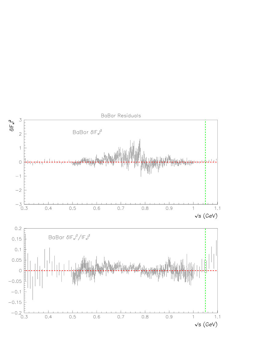
Figure 11: Fit residuals for the BaBar data sample in isolation${}^{\ref{standalone}}$ over the energy range from threshold to 1.05 GeV. The top panel shows the function $\delta|F_{\pi}(s)|^{2}=|F_{\pi}^{BaBar}(s)|^{2}-|F_{\pi}^{fit}(s)|^{2}$; the bottom panel displays the distribution $\delta|F_{\pi}(s)|^{2}/|F_{\pi}^{fit}(s)|^{2}$. The vertical dashed lines indicate the upper end of the fitted spectrum.

Another effect, already noted in [13], is exhibited by Eqs. (11) : the ratio $f_{\rho\gamma}(s)/f_{\rho W}$ becomes $s$–dependent, which is an important difference between $\tau$ decays and $e^{+}e^{-}$ annihilations absent from all previous studies, except for [7]. Figure 11 in [13] shows that the difference between $f_{\rho\gamma}(s)$ and $f_{\rho W}$ is at the few percent level.

2.5 The Pion Form Factor

Here, we only remind the BHLS form of the pion form factor in $\tau$ decay and in $e^{+}e^{-}$ annihilation and refer the interested reader to [13] for detailed information on the other channels. The pion form factor in the $\tau^{\pm}$ decay to $\pi^{\pm}\pi^{0}\nu_{\tau}$ can be written :

$$F_{\pi}^{\tau}(s)=\left[1-\frac{a}{2}(1+\Sigma_{V})\right]-\frac{ag}{2}(1+\Sigma_{V})F_{\rho}^{\tau}(s)\frac{1}{D_{\rho}(s)}~{},$$ (12)

where $a$ and $g$ are the basic HLS parameters [15] already encountered; $\Sigma_{V}$ is one of the isospin breaking parameters introduced by the (extended) BKY breaking scheme. The other quantities are :

$$\left\{\begin{array}[]{lll}\displaystyle F_{\rho}^{\tau}(s)=f_{\rho}^{\tau}-\Pi_{W}(s)~{},\\[14.22636pt] \displaystyle D_{\rho}(s)=s-m^{2}_{\rho}-\Pi_{\rho\rho}^{\prime}(s)~{},\\[14.22636pt] \displaystyle f_{\rho}^{\tau}=agf_{\pi}^{2}(1+\Sigma_{V})~{}~{}~{},~{}~{}m^{2}_{\rho}=ag^{2}f_{\pi}^{2}(1+\Sigma_{V})~{},\end{array}\right.$$ (13)

where $\Pi_{W}(s)$ and $\Pi_{\rho\rho}^{\prime}(s)$ are, respectively, the loop correction to the $\rho^{\pm}-W^{\pm}$ transition amplitude and the charged $\rho$ self–mass (see [13]).

The pion form factor in $e^{+}e^{-}$ annihilation is more complicated and writes :

$$F_{\pi}^{e}(s)=\left[1-\frac{a}{2}(1+\Sigma_{V}+\frac{h_{V}\Delta_{V}}{3})\right]-F_{\rho\gamma}^{e}(s)\frac{g_{\rho\pi\pi}}{D_{\rho}(s)}-F_{\omega\gamma}^{e}(s)\frac{g_{\omega\pi\pi}}{D_{\omega}(s)}-F_{\phi\gamma}^{e}(s)\frac{g_{\phi\pi\pi}}{D_{\phi}(s)}~{},$$ (14)

where $g_{\rho\pi\pi}$, $g_{\omega\pi\pi}$ and $g_{\phi\pi\pi}$ can be read off Eq. (9) and the $F_{V\gamma}^{e}$ are given by :

$$F_{V\gamma}^{e}(s)=f_{V\gamma}(s)-\Pi_{V\gamma}(s)~{}~{},~{}~{}(V=\rho^{0}_{R},~{}\omega_{R},~{}\phi_{R})~{}~{},$$ (15)

with the $f_{V\gamma}(s)$ given by Eqs. (11) above and the $\Pi_{V\gamma}(s)$ being loop corrections [13]. $D_{\rho}(s)=s-m^{2}_{\rho}-\Pi_{\rho\rho}(s)$ is the inverse $\rho^{0}$ propagator while $D_{\omega}(s)$ and $D_{\phi}(s)$ are the modified fixed width Breit–Wigner functions defined in [13]; these have been chosen in order to cure the violation of $F_{\pi}(0)=1$ produced by the usual fixed width Breit–Wigner approximation formulae.

2.6 IB Distortions of the Dipion $\tau$ and $e^{+}e^{-}$ Spectra

IB effects in the $\pi\pi$ channel are of various kinds. In the breaking model developed in [13] and outlined just above, the IB effects following from the neutral vector meson mixing, together or with the photon (see also [7]), are dynamically generated from the HLS Lagrangian. The most relevant effects have been reminded in Subsections 2.3 and 2.4 for the $\pi\pi$ channel. Indeed, Eq. (9) exhibits the generated coupling of the $\omega$ and $\phi$ mesons to a pion pair and Eqs. (10) and (11) show how the $V-\gamma$ couplings are modified by the extended BKY breaking and vector mixing mechanisms. Therefore, in principle, all breaking effects of concern for $e^{+}e^{-}$ annihilations are exhausted.

Some IB effects affecting the dipion $\tau$ spectrum are also generated by the breaking mechanism, which modifies the $W-\rho^{\pm}$ transition amplitude and the $\rho^{\pm}\pi^{\mp}\pi^{0}$ coupling. In some sense, the breaking mechanism decorrelates the universal coupling $g$ as it occurs in the anomalous sector from those in the non–anomalous sector, where $g$ appears in combinations reflecting IB effects, like $g(1+\Sigma_{V})$ for the simplest form [13].

On the other hand, and as a general statement, the effects generated by the pion mass difference $m_{\pi^{\pm}}-m_{\pi^{0}}$ do not call for any specific IB treatment, as the appropriate pion masses are utilized at the corresponding places inside the model formulae derived from BHLS; this concerns, in particular, the pion 3–momentum which appears, for instance, in the phase space terms of the charged and neutral $\rho$ widths.

However, there are IB breaking effects in $\tau$ decay, which have not yet been taken into account. Indeed, known distortions of the dipion $\tau$ spectrum relative to $e^{+}e^{-}$ are produced by the radiative corrections due to photon emission. The long distance effects have been calculated in [56, 57, 58, 59, 60, 61] and the short distance contributions in [62, 63, 64, 65].

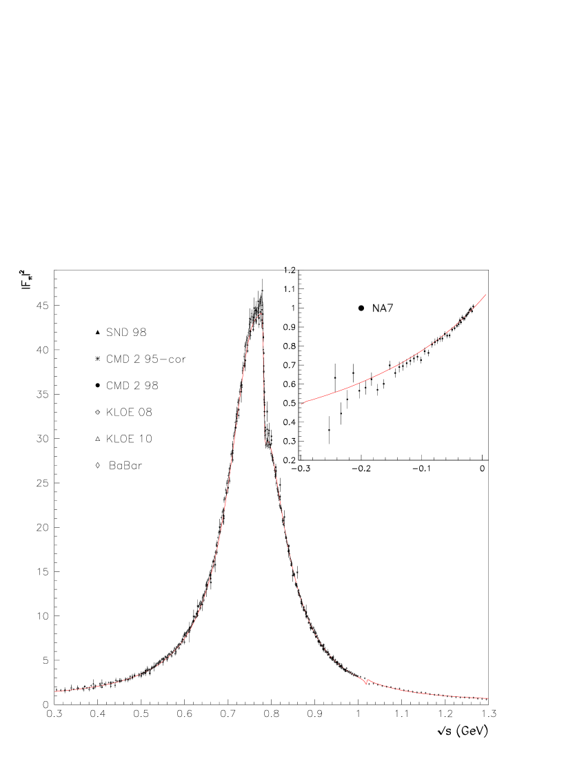
Figure 2: The Pion Form Factor $prediction$ based on $\tau$ data and PDG information. The most important experimental data are superimposed; they do not influence the predicted curve.

We have adopted the corresponding corrections, $G_{EM}(s)$ and $S_{EW}~{}(=1.0235\pm 0.0003)$, respectively, as specified in [13]. In Ref. [59] the contribution of the sub-process $\tau\to\omega\pi^{-}\nu_{\tau}(\omega\to\pi^{0}\gamma)$ has been evaluated to substantially shift the correction $G_{EM}(s)$ (see Fig. 2 in [60]). This sub-process has been subtracted in the Belle data [23] which supposes that the corresponding correction has not to apply. Hence, we applied to the three dipion $\tau$ spectra the correction as given in [56], as in our previous analysis [13].

These IB corrections distort the dipion spectra from the $\tau$ decay. They are accounted for by submitting to the global fit the experimental dipion $\tau$ distributions [21, 22, 23] using the HLS expression for $d\Gamma_{\pi\pi}(s)/ds$ (see Eqs. (73) and (74) in [13] and the present Eq. (14)) corrected – as usual – in the following way :

$${\cal B}_{\pi\pi}\frac{1}{N}\frac{dN(s)}{ds}=\displaystyle\frac{1}{\Gamma_{\tau}}\frac{d\Gamma_{\pi\pi}(s)}{ds}S_{EW}G_{EM}(s)$$ (16)

where $\Gamma_{\tau}$ is the full $\tau$ width and ${\cal B}_{\pi\pi}$ its branching fraction to $\pi^{\pm}\pi^{0}\nu_{\tau}$, both extracted from the RPP [24]. Indeed, as our fitting range is bounded by 1.05 GeV, both pieces of information are beyond the scope of our model. These corrections represent, by far, the most important corrections specific of the $\tau$ decay not accounted for within the HLS framework.

Another source of isospin breaking which may distort the $\tau$ spectrum compared to $e^{+}e^{-}$ is due to the $\rho$ mass difference $\delta M_{\rho}=m_{\rho^{\pm}}-m_{\rho^{0}}$. We note that the Cottingham formula, which provides a rather precise prediction of the $m_{\pi^{\pm}}-m_{\pi^{0}}$ electromagnetic mass difference, predicts for the $\rho$ an electromagnetic mass difference :

$$\delta M_{\rho}\equiv m_{\rho^{\pm}}-m_{\rho^{0}}\simeq\frac{1}{2}\frac{\Delta m^{2}_{\pi}}{M_{\rho^{0}}}\simeq 0.814~{}\mbox{MeV}~{}~{}.$$

In principle, within the HLS model a $\rho^{0}-\rho^{\pm}$ mass shift is also generated by the Higgs-Kibble mechanism (corresponding to the well known shift $\delta M^{2}=M_{Z}^{2}-M_{W}^{2}=g^{\prime 2}\,v^{2}/4$ in the Electroweak Standard Model). In the HLS model $m^{2}_{\rho^{\pm}}=a\,f_{\pi}^{2}\,g^{2}$ while $m^{2}_{\rho^{0}}=a\,f_{\pi}^{2}\,(g^{2}+e^{2})$ due to $\rho^{0}-\gamma$ mixing. This leads to a Higgs-Kibble shift of about $m_{\rho^{0}}-m_{\rho^{\pm}}\simeq\frac{e^{2}}{2g}\sqrt{a}\,f_{\pi}\sim 1~{}\mbox{MeV}$ (see [15]), which essentially compensates the electromagnetic shift obtained from the Cottingham formula. In addition, the masses are subject to modifications by further $\rho-\omega-\phi$ mixing effects, obtained from diagonalizing the mass matrix after including self-energy effects. The mentioned effects have been estimated in [57] and lead to :

$$-0.4~{}\mbox{MeV}<m_{\rho^{0}}-m_{\rho^{\pm}}<+0.7~{}\mbox{MeV}\,.$$

When evaluating the anomalous magnetic moment from $\tau$ data, several choices have been made; for instance, the analysis in [8] assumes $\delta M_{\rho}\simeq 1.0\pm 0.9~{}\mbox{MeV}$, while Belle [23] preferred $\delta M_{\rho}\simeq 0.0\pm 1.0~{}\mbox{MeV}$.

In our study, we followed Belle and have adopted $\delta M_{\rho}\simeq 0\pm 1~{}\mbox{MeV}$, consistent with the estimate by Bijnens and Gosdzinsky just reminded and with most experimental values reported in the RPP [24]. As noted elsewhere [20, 13], based on the available data, auxiliary HLS fits do not improve by letting $\delta M_{\rho}$ floating. This justified reducing the model freedom by fixing this additional parameter to 0.

Yet another source of isospin breaking which may somewhat distort the $\tau$ dipion spectrum compared to its $e^{+}e^{-}$ partner is the width difference $\delta\Gamma_{\rho}=\Gamma_{\rho^{0}}-\Gamma_{\rho^{\pm}}$ between the charged and the neutral $\rho$; however, this can be expected to be small as the accepted average [24], $\delta\Gamma_{\rho}=(0.3\pm 1.3)$ MeV, is consistent with 0.

The expected dominant contribution to $\delta\Gamma_{\rho}$, comes from the radiative $\rho$ decays $\delta\Gamma_{\rho}^{\gamma}=\Gamma(\rho^{0}\to\pi^{+}\pi^{-}\gamma)-\Gamma(\rho^{\pm}\to\pi^{\pm}\pi^{0}\gamma)$. A commonly used estimation [58, 23] for this unmeasured quantity is $\delta\Gamma_{\rho}^{\gamma}=0.45\pm 0.45$ MeV; other values have been proposed, the largest one [8] being $\delta\Gamma_{\rho}^{\gamma}\simeq 1.82\pm 0.18$ MeV. However, summing up all contributions always leads to $\delta\Gamma_{\rho}$ in accord with the RPP average.

Usually, the evaluation of the ($\delta M_{\rho}$, $\delta\Gamma_{\rho}$) effects is performed using the Gounaris–Sakurai (GS) parametrization [66] of the pion form factor. However, the GS formula does not parametrize the radiative corrections expected to affect the measurement of the pion form factor. Therefore, the correction for the radiative width may not be well taken into account by just shifting the width in the GS formula. In Refs. [61, 8] an effective shift of $\delta\Gamma_{\rho}^{\gamma}\simeq 1.82~{}\mbox{MeV}$ has been estimated by subtracting $\rho^{+}\to\pi^{+}\pi^{0}\gamma$ in the $\tau$ channel and adding $\rho^{0}\to\pi^{+}\pi^{-}\gamma$ in the $e^{+}e^{-}$ channel. The question is how this affects $|F_{\pi}(s)|^{2}$. Usually one adopts the GS formula to parametrize the undressed data, which is not precisely what is measured. If one assumes the GS formula to represent the dressed data as well, one may just modify the width for undressing the $\tau$ spectrum and redressing the radiative effects in the $e^{+}e^{-}$ channel, as an IB correction.

An increase of the width in the GS formula has two effects. One is to broaden the $\rho$ shape, which results in an increase of the cross section. The second, working in the opposite direction, is to lower the peak cross section. In the standard form of the GS formula (see e.g. CMD-2 [67] or Belle [23]) the second effect wins and one gets a substantial reduction of the muon $g-2$ integral by $\delta a_{\mu}^{\rm had,LO}[\pi\pi,\tau]=(-5.91\pm 0.59)\times 10^{-10}$ [8], a large reduction of the $\tau$-based evaluation. Looking at the Breit-Wigner peak cross section given by

$$\sigma_{\rm peak}=\frac{12\pi\Gamma_{\rho\to ee}\Gamma_{\rho\to\pi\pi}}{M_{\rho}^{2}\Gamma_{\rho\to{\rm all}}^{2}}$$

it is not a priori clear, which of the different widths are affected. If one keeps fixed the branching fractions for $\rho\to ee$ and $\rho\to\pi\pi$, the peak cross section would not change at all. Therefore, the correction for radiative events via the GS parametrization is not unambiguous. In the standard GS parametrization $\Gamma^{\rm GS}_{ee}=\frac{\alpha^{2}\beta^{3}_{\rho}M_{\rho}^{2}}{36\Gamma_{\rho}}\,(1+d\Gamma_{\rho}/M_{\rho})$ ($dM_{\rho}\Gamma_{\rho}=-\Pi^{\rm ren}_{\rho\rho}(0)$) is a derived quantity and depends on $\Gamma_{\rho}$ in an unexpected way. We therefore consider this standard procedure of correcting for radiative decays as not well established.

Auxiliary fits allowing a difference $\delta g$ between the $\rho^{\pm}$ and $\rho^{0}$ couplings, in order to generate a floating $\delta\Gamma_{\rho}$, have been performed. One observed slightly more sensitivity to a free $\delta g$ than to a free $\delta M_{\rho}$, but nothing conclusive enough to depart from $\delta g=0$ while increasing the number of fit parameters and their correlations. Indeed, within the BHLS framework, the $\tau$ data only play the role of an additional constraint and their use is certainly not mandatory, except for testing the ”$e^{+}e^{-}$ vs $\tau$ discrepancy” which has been shown to disappear [13].

Within the set of data samples which are studied by means of the global fit framework provided by BHLS, the single place where the charged $\rho$ meson plays a noticeable role is the $\tau$ dipion spectrum. Taking into account its relatively small statistical weight within this set of data samples, one does not expect to exhibit from global fits a noticeable sensitivity to mass and width differences with its neutral partner.

3 Confronting the Various $e^{+}e^{-}\to\pi^{+}\pi^{-}$ Data Sets

3.1 The Issue

Although the BHLS Lagrangian should be able to describe more complicated hadron production processes, in a first step one obviously has to focus on low multiplicity states, primarily two particle production but also the simplest three particle production channel $e^{+}e^{-}\to\pi^{+}\pi^{-}\pi^{0}$. Four pion production, annihilation to $KK\pi$ …are beyond the scope of the basic setup of the BHLS model. We expect that available data on the lowest multiplicity channels provide a consistent database which allows us to pin down all relevant parameters, such that our effective resonance Lagrangian is able to simultaneously fit all possible low multiplicity channels. In fact, what is considered are essentially all relevant annihilation channels up to the $\phi$; in this energy range the missing channels ($4\pi,5\pi,6\pi,\eta\pi\pi,\omega\pi$) contribute less than 0.3% to $a_{\mu}^{\rm had}$ [13].

Our previous study [13] has actually shown that the following groups of complementary data samples and/or RPP [24] accepted particle properties (mainly complementary branching fractions) support our global fit strategy :

• (i) All $e^{+}e^{-}$ annihilation data into the $\pi^{0}\gamma$, $\eta\gamma$, $\pi^{+}\pi^{-}\pi^{0}$, $K^{+}K^{-}$, $K^{0}\overline{K}^{0}$ final states admit a consistent simultaneous fit,

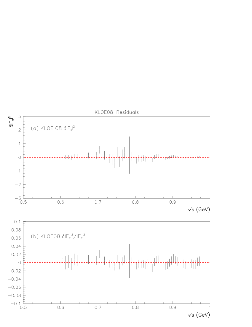
Figure 10: Fit residuals for the KLOE08 data in isolation${}^{\ref{standalone}}$. The top panel shows the function $\delta|F_{\pi}(s)|^{2}=|F_{\pi}^{KLOE08}(s)|^{2}-|F_{\pi}^{fit}(s)|^{2}$; the bottom panel displays the distribution $\delta|F_{\pi}(s)|^{2}/|F_{\pi}^{fit}(s)|^{2}$.

• (ii) The $\tau^{\pm}\rightarrow\nu_{\tau}\pi^{\pm}\pi^{0}$ dipion spectra produced by ALEPH [21], CLEO [22] and BELLE [23], however limited to the energy region where they are in reasonable accord with each other, i.e.$\sqrt{s}\leq 1$ GeV, as can be inferred from Fig. 10 in [13],

• (iii) Some additional partial width from the $P\gamma\gamma$ and $VP\gamma$ decays, which are independent of the annihilation channels listed just above,

• (iv) Some information concerning the $\phi\rightarrow\pi^{-}\pi^{+}$ decay, especially its accepted partial width $\Gamma(\phi\rightarrow\pi^{-}\pi^{+})$ [24]. This piece of information is supposed to partly counterbalance the lack of spectrum for the $e^{+}e^{-}\rightarrow\pi^{+}\pi^{-}$ annihilation in the $\phi$ mass region.

• (v) All the $e^{+}e^{-}\rightarrow\pi^{+}\pi^{-}$ data sets (NSK) collected by the scan experiments mounted at Novosibirsk, especially CMD–2 [26, 27, 28] and SND [29].

They represent a complete reference collection of data samples and lead to fits which do not exhibit any visible tension between the BHLS model parametrization and the data (see for instance Table 3 in [13]). This is worth being noted, as we are dealing with a large number of different data sets collected by different groups using different detectors and different accelerators. The (statistical & systematic) error covariance matrices used within our fit procedure are cautiously constructed following closely the group claims and recommendations. Therefore, the study in [13] leads to think that the $model$ correlations exhibited by BHLS reflect reasonably well the $physics$ correlations expected to exist between the various channels.

However, beside the (NSK) $e^{+}e^{-}\rightarrow\pi^{+}\pi^{-}$ data sets collected in scan mode, there exists now data sets collected using the Initial State Radiation (ISR) method by the KLOE and BaBar Collaborations. All recent studies (see [30, 8], for instance) report upon some ”tension” between them. As this issue has important consequences concerning the estimate of the muon anomalous magnetic moment, it is worth examining if the origin of this tension can be identified and, possibly, substantiated. Besides scan and ISR data, it is also interesting to reexamine [18] the pion form factor data collected in the spacelike region [35, 36] within the BHLS framework; indeed, if valid, these data provide strong constraints on the threshold behavior of the pion form factor and, therefore, an improved information on the muon $g-2$.

3.2 The Analysis Method

The BHLS model has many parameters and a global fit has to be guided by fitting those parameters to those channels to which they are the most sensitive. Obviously resonance parameters of a given resonance have to be derived from a fit of the corresponding invariant mass region. Similarly, the anomalous type interaction responsible for $\pi^{0}\to\gamma\gamma$ or the $\pi\pi\pi$ final state … are sensitive to very specific channels only.

We also have to distinguish the gross features of the HLS model and the chiral symmetry breaking imposed to it. With this in mind, in our approach to comparing the various $e^{+}e^{-}\to\pi^{+}\pi^{-}$ data samples, the $\tau$ decay spectra play a key role since the charged channel is much simpler than the neutral one where $\gamma$, $\rho^{0}$, $\omega$ and $\phi$ are entangled by substantial mixing of the amplitudes, which are not directly observable. In the low energy region, below the kaon pair thresholds and the $\phi$ region, what comes into play is the $\rho^{\pm}$ form factor obtained from the $\tau$ spectra. Together with the isospin breaking due to $\rho^{0}-\omega$ mixing – characterized by the branching fractions $Br(\omega\to\pi^{+}\pi^{-})$ and $Br(\omega\to e^{+}e^{-})$, which in a first step can be taken from the RPP – the $\rho^{\pm}$ form factor should provide a good prediction for the $e^{+}e^{-}\to\pi^{+}\pi^{-}$ channel. Data from the latter can then be used to refine the global fit. This will be our strategy in the following.

The annihilation channels referred to as (i) in the above Subsection as well as the decay information listed in (iii) have little to do with the $e^{+}e^{-}\rightarrow\pi^{+}\pi^{-}$ annihilation channels, except for the physics correlations implied by the BHLS model. On the other hand, as long as one limits oneself to the region $(2m_{\pi},1{\rm~{}GeV})$, there is no noticeable contradiction between the various dipion spectra extracted from the $\tau^{\pm}\rightarrow\nu_{\tau}\pi^{\pm}\pi^{0}$ decay by the various groups [21, 22, 23]. Therefore, it is motivated to examine the behavior of each of the collected $e^{+}e^{-}\rightarrow\pi^{+}\pi^{-}$ data sets, independently of each other, while keeping as $common$ reference the data corresponding to the channels listed in (i) – (iii). Stated otherwise, the data for the channels listed in (i) – (iii), together with the BHLS model, represent a benchmark, able to examine critically any given $e^{+}e^{-}\rightarrow\pi^{+}\pi^{-}$ data sample.

It then only remains to account for isospin breaking effects specific of the $e^{+}e^{-}\rightarrow\pi^{+}\pi^{-}$ channel, in a clearly identified way. A priori, IB effects specific of the $e^{+}e^{-}\rightarrow\pi^{+}\pi^{-}$ annihilation are threefold and cover :

• (j) Information on the decay $\rho^{0}\to e^{+}e^{-}$,

• (jj) Information on the decay $\omega\to\pi^{+}\pi^{-}$,

• (jjj) Information on the decay $\phi\to\pi^{+}\pi^{-}$.

The importance of decay information on $\rho^{0}\to e^{+}e^{-}$ to determine IB effects has been emphasized in only a few previous works [7, 20, 13]. Within the BHLS model, the ratio $f_{\rho\gamma}(s)/f_{\rho W}$ exhibits non–negligible IB effects for this particular coupling (see Fig. 11 in [13]). They amount to several percents in the threshold region quite important for evaluating $g-2$.

There is certainly no piece of information in the data covered by the channels listed in (i) – (iii) above concerning the decay information (jj) or (jjj). In contrast, the vertex $\rho^{0}e^{+}e^{-}$ is certainly involved in all the annihilation channels considered. Imposing the RPP [24] information $\Gamma(\rho^{0}\to e^{+}e^{-})=7.04\pm 0.06$ keV is, nevertheless, legitimate because the channels (i) – (iii) do not significantly constrain the decay width $\rho^{0}\to e^{+}e^{-}$.

For the following discussion we define the branching ratio products $F_{\omega}\doteq\mathrm{Br}(\omega\to e^{+}e^{-})\times\mathrm{Br}(\omega\to\pi^{+}\pi^{-})$ and $F_{\phi}\doteq\mathrm{Br}(\phi\to e^{+}e^{-})\times\mathrm{Br}(\phi\to\pi^{+}\pi^{-})$; these pieces of information are much less model dependent than their separate terms (see Subsection 13.3 in [19]). The RPP accepted information for these products are $F_{\omega}=(1.225\pm 0.071)~{}10^{-6}$ and $F_{\phi}=(2.2\pm 0.4)~{}10^{-8}$.

Two alternative analysis strategies can be followed :

• (k) Use the accepted values [24] for the $\rho^{0}\to e^{+}e^{-}$, $\omega\to\pi^{+}\pi^{-}$ and $\phi\to\pi^{+}\pi^{-}$. These are the least experiment dependent pieces of information. We will be even more constraining by supplementing these $\omega$ and $\phi$ branching ratios by phase information : The so–called Orsay phase concerning the $\omega$ decay and the reported phase of the $\phi\to\pi^{+}\pi^{-}$ amplitude relative to $\rho^{0}\to\pi^{+}\pi^{-}$.

• (kk) Use directly data when possible. Indeed, all relevant IB information carried by $\rho^{0}\to e^{+}e^{-}$ and $\omega\to\pi^{+}\pi^{-}$ can be numerically derived within the BHLS model by the difference between the $\pi^{+}\pi^{-}$ spectra and the dipion spectrum $\pi^{\pm}\pi^{0}$ in the $\tau$ decay; more precisely, using the $\pi^{+}\pi^{-}$ spectrum within the tiny energy region $0.76\div 0.82$ GeV should be enough to derive the relevant IB pieces of information in full consistency with our model.

  As all scan (NSK) $e^{+}e^{-}\rightarrow\pi^{+}\pi^{-}$ data samples [25, 26, 27, 28, 29] and both KLOE data sets (KLOE08 and KLOE10) stop below 1 GeV, the $\phi$ information should be taken from somewhere else, namely from the RPP. Fortunately, the $\phi$ region is now covered by the BaBar data set [33, 34]. Therefore, as soon as the consistency of the $\phi\to\pi^{+}\pi^{-}$ information carried by the BaBar data and by [24, 72] is established, this part of the spectrum could supplement the scan and KLOE data sets.

  Concerning the $\phi\to\pi^{+}\pi^{-}$ information, this second strategy will be used by either taking the [24, 72] information or the BaBar data points between $1.0$ and $1.05$ GeV.

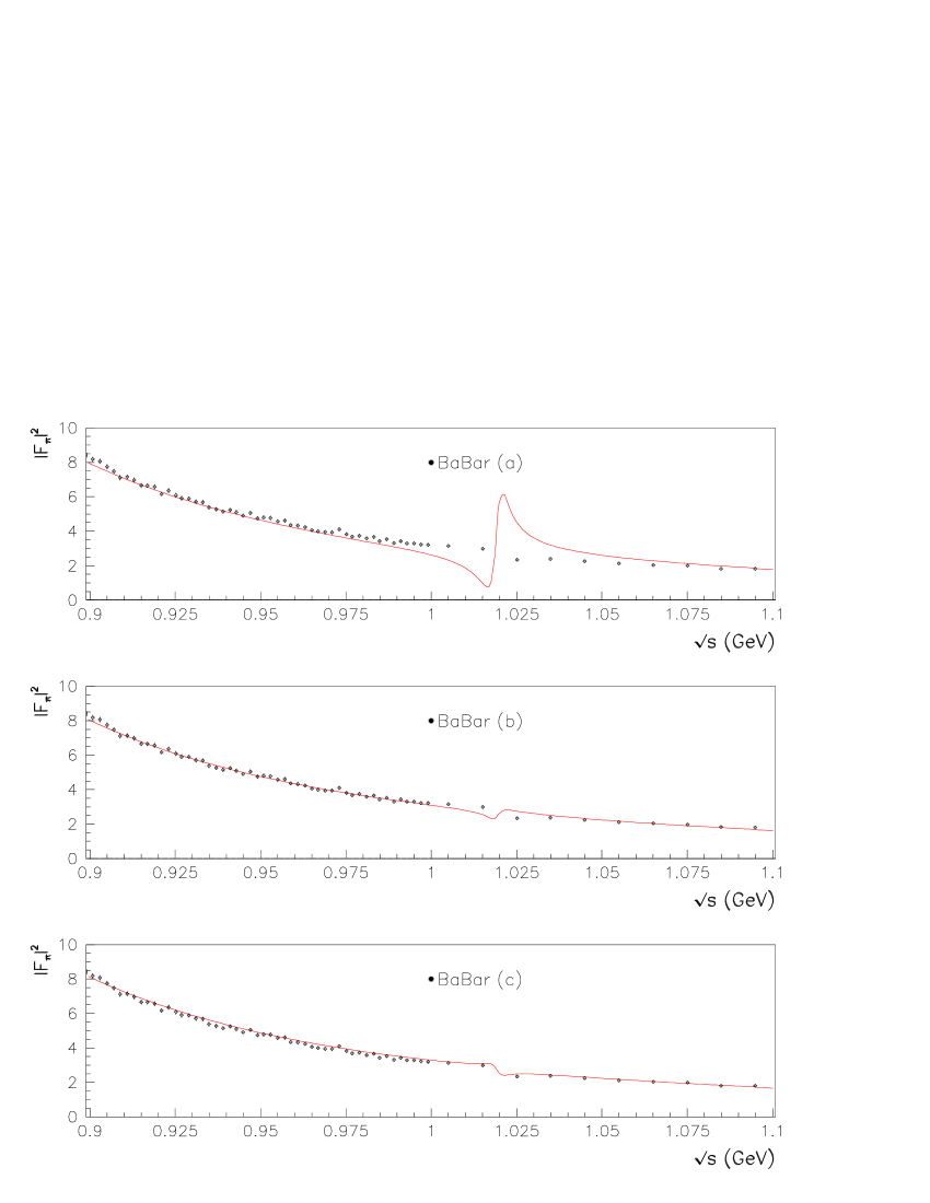
Figure 1: The $e^{+}e^{-}\rightarrow\pi^{+}\pi^{-}$ cross section around the $\phi$ mass together with BaBar data superimposed. The curve in (a) displays the prediction using the RPP $\phi$ decay information computed at the $\phi$ Higgs–Kibble mass; the curve in (b) displays the prediction using the PDG $\phi$ decay information computed at the experimental $\phi$ mass. In (c) the PDG $\phi$ decay information is replaced by the five BaBar data points located between 1. and 1.05 GeV.

3.3 How to Implement $\omega/\phi\to\pi^{+}\pi^{-}$ PDG Information?

The vector meson couplings to $\pi^{+}\pi^{-}$ or $e^{+}e^{-}$ depend on the $s$–dependent ”mixing angles” $\alpha(s)$, $\beta(s)$ and $\gamma(s)$. This does not give rise to any ambiguity as long as one deals with spectra; however, when using the PDG information for vector meson decays, especially to $\pi^{+}\pi^{-}$ or $e^{+}e^{-}$, one has to specify at which value for $s$ each of the vector meson (model) coupling should be evaluated.

Within the HLS model, there are a priori two legitimate choices for the mass of vector mesons; this can either be the Higgs–Kibble (HK) mass which occurs in the Lagrangian after symmetry breaking or, especially for the $\omega$ and $\phi$ mesons, the experimental (accepted) mass as given in the RPP. Prior to the availability of the BaBar data [33], the published $e^{+}e^{-}\rightarrow\pi^{+}\pi^{-}$ cross section data did not include the $\phi$ mass region and, therefore, there was no criterion to check the quality of each possible choice in the $\phi$ mass region. The choice made in the previous studies using the broken HLS model [18, 19, 20, 13] was the $\phi$ HK mass.

As already noted, the broken HLS model, fed with the data listed in i–iv (see Subsection 3.1, above), provides predictions for the pion form factor independently of the measured $e^{+}e^{-}\to\pi^{+}\pi^{-}$ data. This procedure is discussed in detail in the next section. Here we anticipate some results specific to the $\phi$ mass issue.

Fig. (1a) displays the prediction for the pion form factor in the $\phi$ region using the HK mass to estimate the $\phi\pi^{-}\pi^{+}$ coupling constant with the BaBar data superimposed (not fitted); it is clear that the prediction is quite reasonable up to $\simeq 0.98$ GeV as well as above $\simeq 1.05$ GeV. However, it is clearly unacceptable for the mass region in–between. In contrast, using the $\phi$ mass as given in the RPP to extract the $\phi\pi^{-}\pi^{+}$ coupling constant from its accepted partial width [24] provides the spectrum shown in Fig. (1b); this alternate choice is certainly reasonable all along the mass region displayed. Therefore, it is motivated to update our former results [13] by performing the change just emphasized. In order to be complete, it is worth mentioning here a fit result obtained by exchanging the PDG/SND $\phi$ decay information with the BaBar pion form factor data${}^{\ref{bbr_phi}}$ in the range ($1.0\div 1.05$) GeV. The result, given in Fig. (1c), shows that the lineshape of the BaBar pion form factor at the $\phi$ mass can be satisfactorily accommodated. As the exact pole position of the $\phi$ meson is determined by a benchmark independent of the $e^{+}e^{-}\to\pi^{-}\pi^{+}$ process (see Subsection 3), the drop exhibited by Fig. (1c) in the BaBar is perfectly consistent with an expected $\phi$ signal.

4 $\tau$ Predictions of the Pion Form Factor

4.1 $\tau$+PDG Predictions

As mentioned before, the charged isovector $\tau^{\pm}\to\nu_{\tau}\pi^{\pm}\pi^{0}$ dipion spectra are not affected by $\gamma-\rho-\omega-\phi$ mixing and hence are of much simpler structure. Supplemented by the basic $\rho-\omega-\phi$ mixing effects which derive from $SU(2)$ and $SU(3)$ flavor breaking, one has a good starting point to fix the parameters of the BHLS model to predict the process $e^{+}e^{-}\to\pi^{+}\pi^{-}$. Specifically, we are using the data including the channels listed in i-iv of Section 3 together with RPP information relevant to fix the IB effects affecting the pion form factor. This method is named, somewhat abusively $\tau$+PDG.

Specifically, the IB effects encoded in $\mathrm{Br}(\omega\to\pi^{+}\pi^{-})$, $F_{\omega}\doteq\mathrm{Br}(\omega\to e^{+}e^{-})\times\mathrm{Br}(\omega\to\pi^{+}\pi^{-})$ and $F_{\phi}\doteq\mathrm{Br}(\phi\to e^{+}e^{-})\times\mathrm{Br}(\phi\to\pi^{+}\pi^{-})$ are taken from the RPP. For the missing phase information we adopt the result from the fit [70] for the Orsay phase of the $\omega\to\pi^{+}\pi^{-}$ amplitude and the result from SND [72] for the phase of the $\phi\to\pi^{+}\pi^{-}$ amplitude. Following the discussion in the preceding Subsection, the model branching ratios and phases are computed at the vector boson masses accepted by the RPP.

The fit returns a probability of 89.4% with $\chi^{2}/n_{dof}=553.4/596$. The fit quality ($\chi^{2}/n_{points}$) for each of the fitted channels is almost identical to our results in [13] (see the last column in Table 3 therein). Each of the decay partial width extracted from [24] contributes by $\simeq 1$ to the total $\chi^{2}$. It is also worth mentioning that the dipion spectra from [21, 22, 23] are nicely described up to $\sqrt{s}=1$ GeV and provide residual distributions indistinguishable from those shown in Figure 10 of [13]. From this fit, one derives the ($\tau$+PDG) predictions for the pion form factor which can be compared with the various existing $e^{+}e^{-}\rightarrow\pi^{+}\pi^{-}$ data samples.

The overall view of the comparison is shown in Fig. 2. This clearly indicates that the data associated with the channels listed in i–iv, supplemented with a limited PDG information is indeed able to provide already a satisfactory picture of the pion form factor as reported by all experiments having published $e^{+}e^{-}\rightarrow\pi^{+}\pi^{-}$ spectra.

Let us stress that the predicted pion form factor relies on the $\pi^{\pm}\pi^{0}$ spectra provided by ALEPH [21], Belle [23] and CLEO [22] only up to 1.0 GeV. Therefore, the inset in Fig. 2 actually shows the $extrapolation$ of the prediction into the spacelike region with the NA7 data [35] superimposed; this clearly indicates that there is no a priori reason to discard the spacelike data from our data handling. One should also note that the extrapolation of the prediction above the $\phi$ mass is quite reasonable up to $\simeq 1.2\div 1.3$ GeV. This may indicate that the influence of high mass vector mesons is negligible up to this energy region.

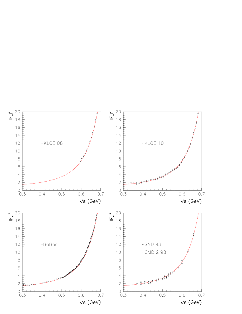
Figure 3: Magnified view of the Pion Form Factor $prediction$ based on $\tau$ data and PDG information; the ($0.3\div 0.7$) GeV region is shown with the indicated data superimposed.

In order to make more precise statements, let us magnify piece wise the information carried by Fig. 2. Thus, Fig. 3 displays the behavior of the various $e^{+}e^{-}\rightarrow\pi^{+}\pi^{-}$ data samples in the ($0.3\div 0.7$) GeV energy region. As a general statement the behavior expected from the existing data samples looks well predicted by the $\tau$+PDG method. A closer inspection allows to infer that the CMD–2 and SND data points (i.e. NSK when used together) are well spread onto both sides of the predicted curve; this property is also shared by the KLOE10 sample. Even if reasonably well described, the KLOE08 and BaBar data samples are lying slightly above the $\tau$+PDG expectations; this difference should vanish when including the $\pi^{+}\pi^{-}$ spectra inside the fit procedure.

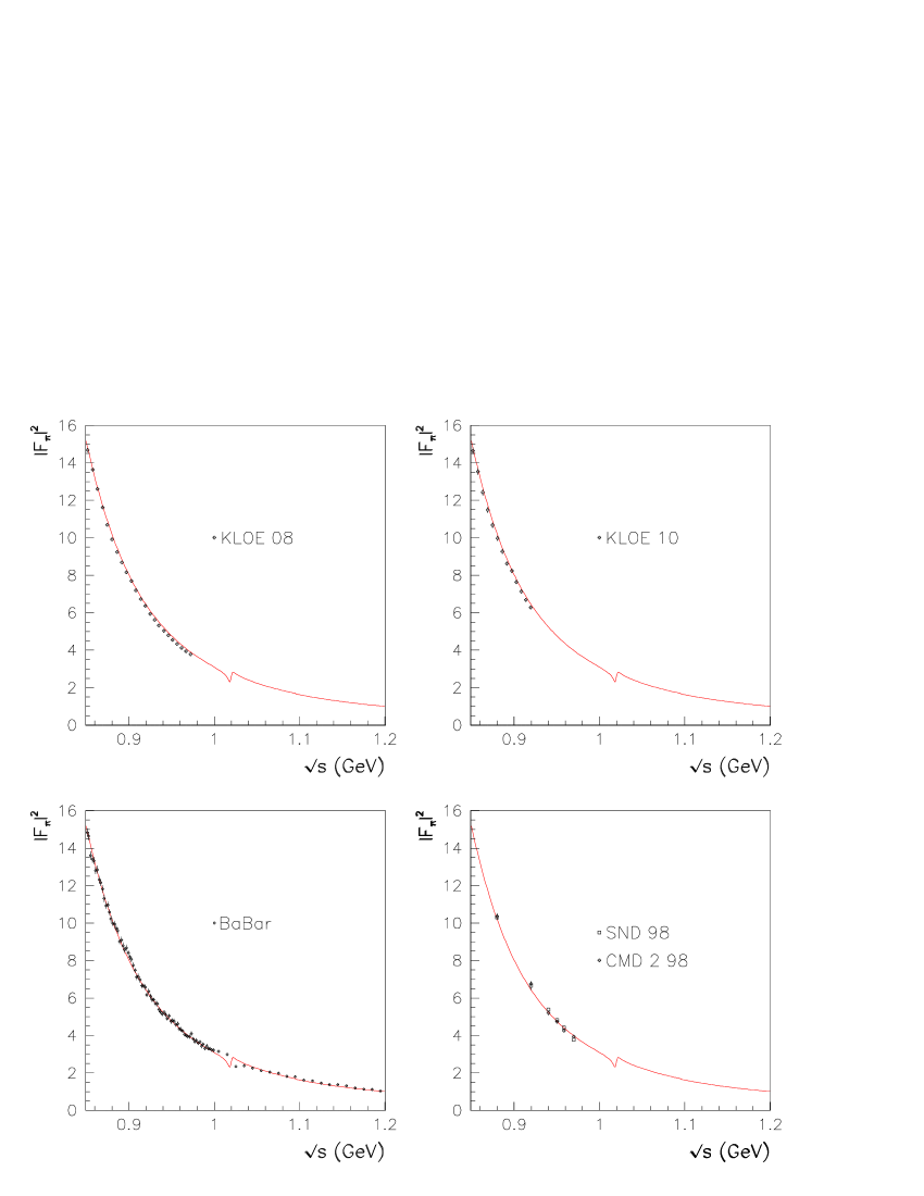
Figure 4: Magnified view of the Pion Form Factor $prediction$ based on $\tau$ data and PDG information; the ($0.85\div 1.2$) GeV region is shown with the indicated data superimposed.

Fig. 4 displays the behavior of the various $e^{+}e^{-}\rightarrow\pi^{+}\pi^{-}$ data samples in the ($0.85\div 1.2$) GeV energy region. Here also the predicted curve accounts well for the data behavior. A closer inspection tells that the sparse NSK data are well described. The BaBar data are also well accounted for all along this energy interval except for the $\phi$ region. As shown by Fig. (1c) above, this can be cured and one can show that the difference is mostly due to the phase for the $\phi\to\pi^{+}\pi^{-}$ amplitude which departs significantly from those provided by SND [72]. One could also note that both KLOE data samples look slightly below the $\tau$+PDG expectations in this region.

One may conclude from Figs. 3 and 4 that our ”$\tau$+PDG” predictions are in good agreement with the data and that a fit using fully these data samples should provide marginal differences between all $\pi^{+}\pi^{-}$ data sets .

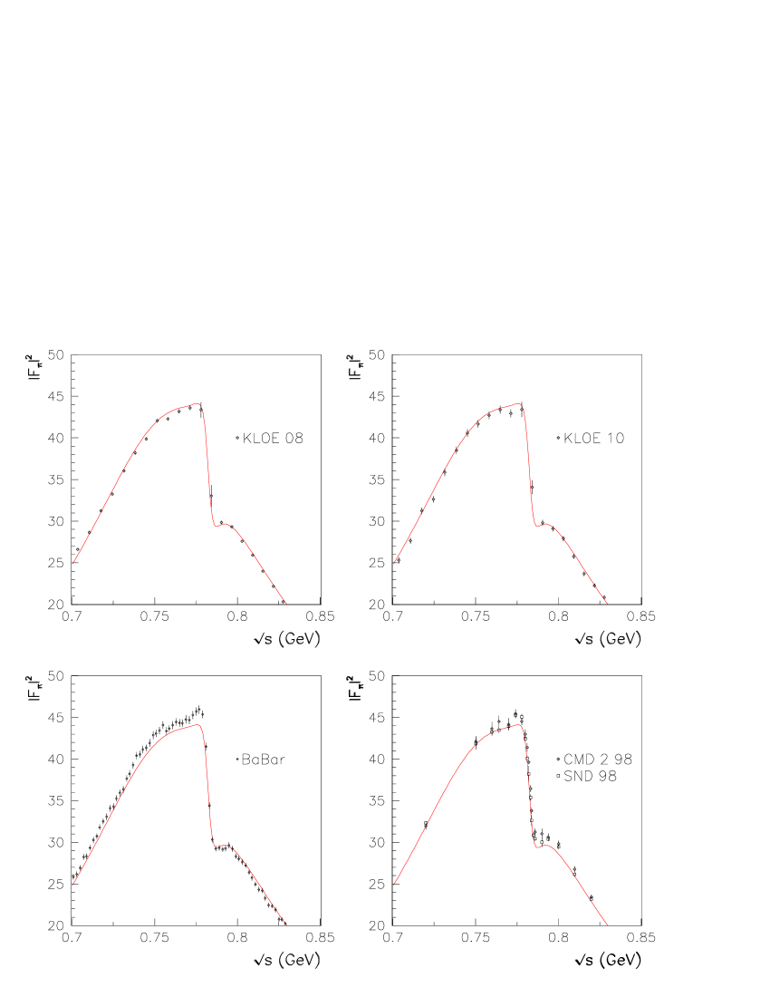
Figure 5: Magnified view of the Pion Form Factor $prediction$ based on $\tau$ data and PDG information; the ($0.7\div 0.85$) GeV region is shown with the indicated data superimposed.

However, the picture becomes quite different in the medium energy region ($0.70\div 0.85$) GeV as illustrated by Figure 5. In this region, our $\tau$+PDG prediction follows almost perfectly expectations${}^{\ref{errors}}$ from both the KLOE08 and KLOE10 data and the detailed lineshape of the $\omega-\rho$ interference region is strikingly reproduced. Paradoxically, the NSK data are slightly less favored – especially around 0.8 GeV – despite their influence on the PDG information used in order to account for IB effects in the $\omega-\rho$ interference region; however, taking into account experimental uncertainties, we already know that a global fit using NSK data is highly successful [13].

In contrast, the behavior of the BaBar data looks inconsistent with the $\tau$+PDG prediction, especially on the low mass side of the interference region. Actually, the observed overestimate of the BaBar spectrum affects the whole region from threshold to the $\omega$ mass but is more important in the range ($0.74\div 0.78$) GeV. At higher energies one observes a reasonable agreement with expectations as well as with both KLOE data sets.

One should also note that the $\omega$ mass and (total) width induced by the data for the $\pi^{0}\gamma$, $\eta\gamma$, $\pi^{+}\pi^{-}\pi^{0}$ final states are in perfect agreement with all the examined data samples; this indicates that the energy calibration around the $\omega$ mass is good for all ISR data samples. Fig. (1c) has already shown that the BaBar energy calibration is also good in the $\phi$ region.

4.2 Predictions Using the $\rho^{0}-\omega$ Interference Region From Data

As stated in Subsection 3.1, one can replace the PDG information for $\omega\to\pi^{+}\pi^{-}$ and $\rho^{0}\to e^{+}e^{-}$ by any pion form factor spectrum limited to the region $(0.75\div 0.82$) GeV. In particular, this turns out to fit $F_{\omega}={\rm Br}(\omega\to e^{+}e^{-})\times{\rm Br}(\omega\to\pi^{+}\pi^{-})$ and the Orsay phase as it comes out from each of the specified data sets.

Concerning the $\phi\to\pi^{+}\pi^{-}$ mode, one can also check the BaBar data [33, 34] versus the SND datum [72]. This will be discussed below when reporting on fitting the whole spectra (see Subsection 5.2.1).

Data Sample	Local Fit
	$F_{\omega}\,10^{6}$	Orsay Phase (degrees)	Prob. (%)	$\chi^{2}/n_{\pi^{+}\pi^{-}}$
Reference values [29, 70]	$1.225\pm 0.071$	$104.70\pm 4.10$	–	–
$\tau$ + PDG	$1.157\pm 0.053$	$108.92\pm 2.36$	89.4%	–
$\tau$ + NSK [27, 29]	$1.219\pm 0.043$	$106.71\pm 0.25$	90.0%	52/47
$\tau$ + KLOE08 [31]	$1.076\pm 0.041$	$110.44\pm 1.24$	87.8%	18/11
$\tau$ + KLOE10 [32]	$0.973\pm 0.045$	$113.62\pm 1.63$	92.7%	11/11
$\tau$ + BaBar [33]	$1.780\pm 0.011$	$107.50\pm 0.19$	54.4%	67/35

Table 1: Fit results for $F_{\omega}\doteq{\rm Br}(\omega\to e^{+}e^{-}){\rm Br}(\omega\to\pi^{+}\pi^{-})$ and for the Orsay phase (in degrees) using only the $(0.75\div 0.82$) GeV energy region of each $\pi^{+}\pi^{-}$ data sample. The fit is done following the (local) procedure sketched in Subsection 4.2; we use ${\rm Br}(\omega\to\pi^{+}\pi^{-})=(1.53\pm 0.13)\%$ [24] and the Orsay phase from [70] as input values for the “$\tau$ + PDG” fit. The probabilities are those of the global fit; the last data column shows the contribution of each $\pi^{+}\pi^{-}$ data set to the total $\chi^{2}$ and gives the corresponding number of data points.

Using the RPP recommended value for ${\rm Br}(\omega\to\pi^{+}\pi^{-})$ and the Orsay phase information from [70] yields a value for $F_{\omega}$ in good correspondence with expectations, as clear from the entry $\tau$ + PDG in Table 1. Using NSK data or any of both KLOE samples, instead of the PDG information, does not lead to predicted curves substantially different from their analogue already shown and commented upon in the previous Subsection. Interesting parameter values have been extracted from global fits using only the $(0.75\div 0.82$) GeV region from the NSK and KLOE spectra for $e^{+}e^{-}\to\pi^{+}\pi^{-}$ and are reported in Table 1; they are in reasonable agreement with the reported branching ratio product $F_{\omega}$ [29] and the Orsay phase [70, 71] as well. Indeed, taking the RPP $F_{\omega}$ value as reference, our estimates using the 70 MeV interval surrounding the interference region are at $0.1\sigma$, $1.8\sigma$ and $3.0\sigma$ for respectively the NSK [27, 29], KLOE08 [31] and KLOE10 [32] data samples. The difference between the RPP recommended value for $F_{\omega}$ and our entry for NSK also tells that the BHLS parametrization and the more standard form factor lineshape used by SND [29] provide almost identical values for $F_{\omega}$.

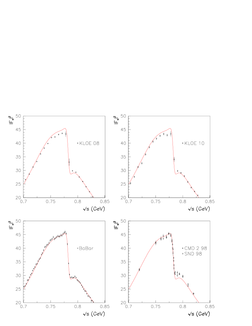
Figure 6: The Pion Form Factor $prediction$ based on $\tau$ data and the ($0.76\div 0.82$) GeV region of the BaBar spectrum [33]; the ($0.7\div 0.85$) GeV region is shown with the indicated data superimposed.

As far as BaBar data are concerned, the situation looks different and the most relevant piece of information is provided in Figure 6. This proves that the largest difference between BaBar data and the other analogous data samples [27, 29, 31, 32] is the $F_{\omega}$ information inherent to the BaBar data. Clearly, Table 1 shows that the BaBar value for $F_{\omega}$ is off from its recommended value by $(7\div 8)\sigma$. This strong disagreement is substantiated by comparing Figures 5 and 6.

Table 1 also reports the fit probability for each of the examined configurations. With about 90% probabilities, the ”$\tau$+PDG” prediction and the NSK, KLOE08 and KLOE10 (global) fits exhibit a full consistency with the rest of our benchmark (i.e. all other annihilation channel physics). The agreement of this with BaBar data, even limited to such a tiny interval, is found much poorer and exhibits a clear tension between $F_{\omega}^{BaBar}$ and the rest of the (non–$\pi^{+}\pi^{-}$) physics accessible to the HLS model.

Additional pieces of information are provided in the last data column of Table 1 which complements the global fit probabilities. These are the values for $\chi^{2}/n_{\pi^{+}\pi^{-}}$ for each of the various $\pi^{+}\pi^{-}$ data samples, $n_{\pi^{+}\pi^{-}}$ being the number of data points included in the fitted energy range (i.e. $(0.75\div 0.82)$ GeV).

4.3 Isospin Breaking Effects in the BHLS Model : Comments

It follows from the developments just above that the BHLS model fed with a limited number of accepted values for some IB pieces of information is indeed able to provide a quite satisfactory prediction for the $e^{+}e^{-}\to\pi^{+}\pi^{-}$ cross section once the $\tau$ spectra are considered. This gives support to our breaking model, especially to the $s$–dependent vector meson mixing mechanism.

The prediction is found in accord with the scan (NSK) data samples and with both KLOE data sets. Indeed, the predicted lineshape strikingly follows the central values from both KLOE data samples; for the scan data, the prediction based on PDG information is good but not as good as for the KLOE data. However, changing the PDG requested IB information by less than 1 $\sigma$ – as following from a mere comparison of the first and second lines in Table 1 – leads to a perfect description of the NSK spectra over the whole available energy range [13]. In contrast, the RPP branching fraction product $F_{\omega}$ has to be changed by about $7\sigma$ in order to yield a comparable description of the BaBar [33] data.

Basically, our approach is a $\tau$ based prediction of $\pi^{+}\pi^{-}$ spectra; it relies on the consistency of several different physics channels, the $\tau$ spectra and on a model of isospin symmetry breaking (IB). In fine, our breaking model does not carry IB parameter values plugged in from start, but yields the numerical IB effects in a data driven mode. It is thus interesting to examine the consequences of this $\tau$ (and global) based approach on the muon $g-2$ estimated value. For this purpose, it is worth stressing that the $\tau$ based estimates given just below – and later – are $not$ computed by integrating the $\tau$ spectra (and adding corrections like in [23, 8], for instance), but by integrating the $e^{+}e^{-}$ cross sections they allow to reconstruct through the global BHLS framework.

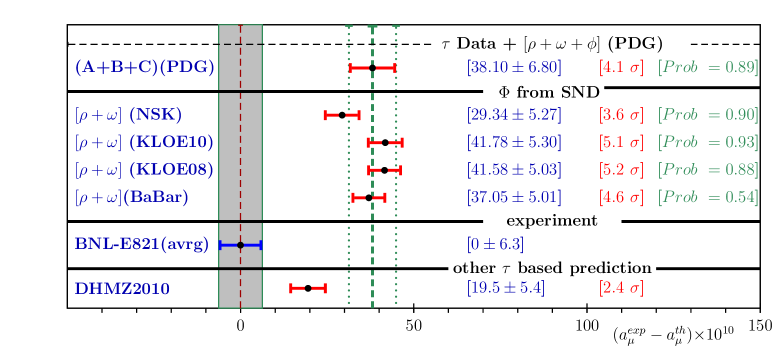
Figure 7: $\tau$ based estimates using a global fit of the BHLS model (see Section 4). The first two numbers in each line display resp. the central value and the r.m.s. of $\Delta a_{\mu}=a_{\mu}^{exp}-a_{\mu}^{th}$. The last two numbers give resp. the distance to the BNL measurement and the fit probability – essentially dominated by the non $\pi^{+}\pi^{-}$ data. The lower probability found when using the BaBar data, even in the limited energy region involved ($[0.76\div 0.82]$ GeV), exhibits the tension of this data sample relative to the rest of the physics considered.

This is what is shown in Figure 7. The first line displays the result derived from the “$\tau$+PDG” fit. The four following lines are obtained by replacing the $\rho$ and $\omega$ IB information by the $0.76\div 0.82$ GeV region of the quoted data sets. The line named BNL displays the experimental result [39, 40] and the last line shows the $\tau$ based estimate from [8]. The last data column in Figure 7 gives the probability of the corresponding fits.

It is clear that all methods used to include IB effects within our $\tau$ based approach give consistent results, all distant from the BNL measurement at the $4\sigma$ level. The associated probabilities indicate the quality of the fits from where they are derived.

5 Global Fits Using the $e^{+}e^{-}\to\pi^{+}\pi^{-}$ Spectra

As in our previous analysis [13], we have performed global fits using simultaneously all $e^{+}e^{-}$ annihilation data into the $\pi^{0}\gamma$, $\eta\gamma$, $\pi^{+}\pi^{-}\pi^{0}$, $K^{+}K^{-}$, $K^{0}\overline{K}^{0}$ final states, the dipion spectra collected in the decay of the $\tau$ lepton [21, 23, 22] and the decay information listed in Subsection 3.1. We also use the RPP $\phi$ decay properties in the (updated) way emphasized in Subsection 3.3.

For what concerns the $e^{+}e^{-}\to\pi^{+}\pi^{-}$ data included into the global fit procedure, we have performed fits using separately the NSK, KLOE08 and KLOE10 data samples. Global fits have also been performed for the BaBar dipion spectrum restricted to the range of validity of our BHLS model. Two options have been considered, using BaBar data up to 1 GeV supplemented by $\phi\to\pi^{+}\pi^{-}$ decay properties from the RPP or using the BaBar data up to 1.05 GeV, thus including its $\phi$ region and avoiding the need of using the RPP information about the $\phi$.

In all cases, the errors (and the $\chi^{2}$) were constructed following the information published/ recommended by the experimental groups who collected these data. For instance, concerning the scan data samples, the full covariance matrix is generally constructed by adding the systematic error covariance matrix $V_{syst}$ to the (diagonal) statistical covariance $V_{stat}$ constructed from the tabulated uncertainties as described in [19] (see Section 6 therein); $V_{syst}$ is constructed assuming the reported systematic errors bin–to–bin correlated . Nevertheless, for the rather imprecise $e^{+}e^{-}\to(\pi^{0}/\eta)\gamma$ data, taking into account the large magnitude of the reported systematics, the systematic and statistical errors were simply added in quadrature. For the $e^{+}e^{-}\to\pi^{+}\pi^{-}\pi^{0}$ data, we dealt with depending on the level of precision of the relevant data sample (see Subsection 2.2.3 in [20] for more information).

For the $\tau$ data, as both $V_{syst}$ and $V_{stat}$ are publicly available [21, 22, 23], one only has to add them up, as already performed for the study in [13]. For the BaBar sample, the systematic uncertainties on the cross section are given (as a function of $\sqrt{s}$) in Table V from [34] and are imposed to be 100 % bin–to–bin correlated (following Section F in [34]). Writing, for definiteness, each of these uncertainty functions as $f(s_{i})$, for the data point $m_{i}$ located at $\sqrt{s_{i}}$, the $(i,j)$ entry of the $V_{syst}$ matrix is given by the sum of the various $f(s_{i})f(s_{j})m_{i}m_{j}$.

For both the KLOE08 and KLOE10 data samples [31, 32], the KLOE Collaboration provides basically the same information as BaBar and therefore, we simply have to proceed likewise.

Moreover, the various $\pi^{+}\pi^{-}$ data sets collected by CMD–2 and SND [27, 28, 29] on the one hand and the older data samples from [25] on the other hand, both carry common bin–to–bin $and$ sample–to–sample correlated uncertainties estimated resp. to 0.4% and $\simeq 1$%. As in our previous studies [20, 13], this effect is accounted for in the minimization code. These are the most important reported correlations of this type within the scan data [74].

We have also performed global fits using combinations of these individual $\pi^{+}\pi^{-}$ data samples. In this case, the contributions of the NSK and KLOE10 data to the total $\chi^{2}$ were left unweighted as their own $\chi^{2}/n$ contribution is always of the order 1 in fits using each of them in “isolation”. In contrast, in such combinations involving the KLOE08 and/or BaBar data, the contribution of each of these to the total $\chi^{2}$ was weighted by the ratio $f_{M}=n_{M}/\chi^{2}_{M}$ (M= KLOE08, BaBar) where $\chi^{2}_{M}$ is the $\chi^{2}$ of the M data set obtained in the best fit using only M as $e^{+}e^{-}\to\pi^{+}\pi^{-}$ data set; $n_{M}$ is the corresponding number of data points. In fits involving the spacelike data [35, 36], the corresponding weight was also used.

For definiteness, when relevant, we have used $f_{NSK}=f_{KLOE10}=1$, $f_{KLOE08}=60/90\simeq 0.67$, $f_{BaBar}=270/346\simeq 0.78$ and $f_{space}=59/85\simeq 0.69$. These weights have been varied and it has been found that the sensitivity of the physics results to their precise value is marginal; the main virtue of these weights is to provide probabilities not too much ridiculous. On the other hand, as a matter of principle, when results are displayed which have been obtained using weights, it is quite generally for the reader’s information. We have preferred being conclusive by only relying on the largest data set combinations which do not call for any reweighting. Indeed, this simply reflects that global fit probabilities do not raise any objection to trusting the uncertainties as they are reported together with each of the used data sets.

This method, turns out to consider each data set as a global object, rather than defining local ($s$–dependent) averages as done by others [6]. This method looks better adapted to the global fit method which provides a quality check reflecting the behavior of each $e^{+}e^{-}\to\pi^{+}\pi^{-}$ data set within the global context of a large number of physics channels. Indeed, doing local averages would prevent to detect discrepancies originating from some given data set only. On the other hand, within a global framework as BHLS, such a method would lead to fit parameter values modified in a completely uncontrolled way. It is the reason why our final results will only rely on sample combinations which do not call for any reweighting (i.e. necessarily going beyond experimentally reported uncertainty information).

For completeness, it is also worth noting that the $\chi^{2}$ contributions of the – more than 40 – data sets associated with all the other channels were always left unweighted.

A feature common to all fits using the $e^{+}e^{-}\to\pi^{+}\pi^{-}$ data sets in “isolation” or combined is that the individual $\chi^{2}$ contributions associated with the other channels ($\pi^{0}\gamma$, $\eta\gamma$, $\pi^{+}\pi^{-}\pi^{0}$, $K^{+}K^{-}$, $K^{0}\overline{K}^{0}$, …) were only marginally affected by the specific choice of $e^{+}e^{-}\to\pi^{+}\pi^{-}$ data submitted to fit. Their typical values are almost identical to what can be found in the last data column of Table 3 in [13]; more precisely, the $\chi^{2}$ value provided by each of these channels never varies by more than a few percents. Let us remind that the number of data points submitted to fit – beside the $e^{+}e^{-}\to\pi^{+}\pi^{-}$ data – is $\simeq 600$ when working within the configuration B defined in [13] ($\simeq 675$ within configuration A).

5.1 Salient Features of the Various $e^{+}e^{-}\to\pi^{+}\pi^{-}$ Spectra

We have performed several tens of fits of the various $e^{+}e^{-}\to\pi^{+}\pi^{-}$ spectra in “standalone” mode${}^{\ref{standalone}}$ and/or combined. It does not look useful to report on each fit in detail. Instead of overwhelming the reader with unnecessary information and plots, we have preferred focusing on the salient features of their behavior within the global fit context. Beside the fit properties of the full spectra (up to 1 GeV, generally), this covers the muon anomalous magnetic moment value and the behavior at the $\omega$ mass, more precisely the value for $F_{\omega}={\rm Br}(\omega\to e^{+}e^{-})\times{\rm Br}(\omega\to\pi^{+}\pi^{-})$. The first of these topics will be addressed in a separate Section below. Concerning the second topic, we remind that the value for $F_{\omega}$ expected from the RPP is $(1.225\pm 0.071)~{}10^{-6}$.

On the other hand, we do not enter into much detail concerning the effects of the spacelike data, always used weighted in this paper; we limit ourselves to mentioning that they never modify the fit qualities in a significant way.

5.1.1 “Standalone” Fits of the $e^{+}e^{-}\to\pi^{+}\pi^{-}$ Spectra

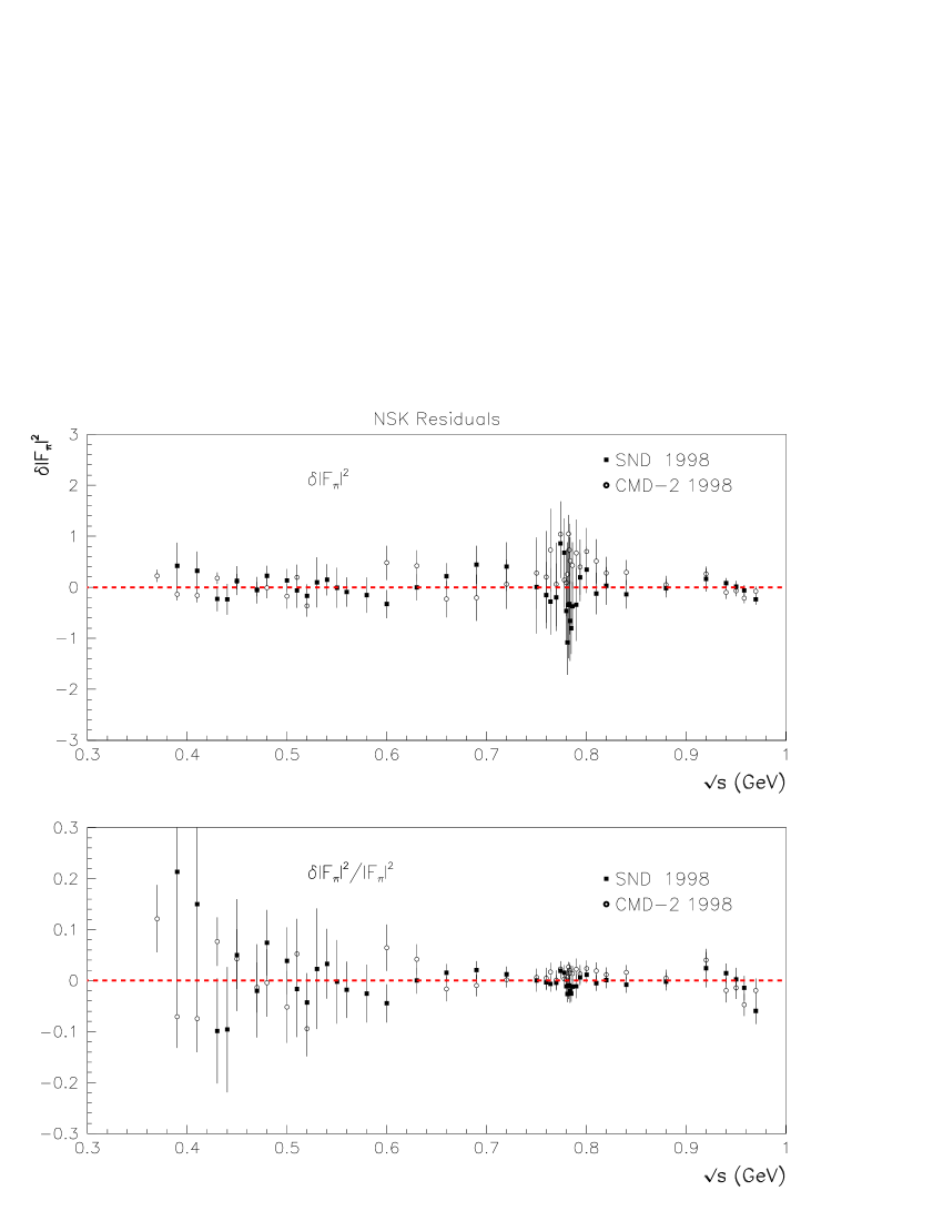
Figure 8: Fit residuals for the CMD–2 and SND data samples (NSK) in isolation${}^{\ref{standalone}}$. The top panel shows the function $\delta|F_{\pi}(s)|^{2}=|F_{\pi}^{NSK}(s)|^{2}-|F_{\pi}^{fit}(s)|^{2}$; the bottom panel displays the distribution $\delta|F_{\pi}(s)|^{2}/|F_{\pi}^{fit}(s)|^{2}$.

When using only${}^{\ref{standalone}}$ the (unweighted) NSK data, the fit returns $\chi^{2}_{NSK}/N_{\pi^{+}\pi^{-}}=128.30/127$ and a global fit probability of 96.3%. The fit residuals are displayed in the top panel of Fig. 8 and the fractional deviations from the fitting function in the bottom panel. Taking into account the uncertainties, both plots do not exhibit any significant departure from flatness. The fit residual distributions of the ALEPH, CLEO and Belle dipion spectra also submitted to fit in the present case are rigorously given by Fig. 10 in [13], where the fit also extends over the energy region from threshold to 1 GeV. Therefore, one indeed observes flat residual distributions and flat fractional deviations from the fitting functions simultaneously in the $e^{+}e^{-}$ and $\tau$ channels as already claimed in [13].

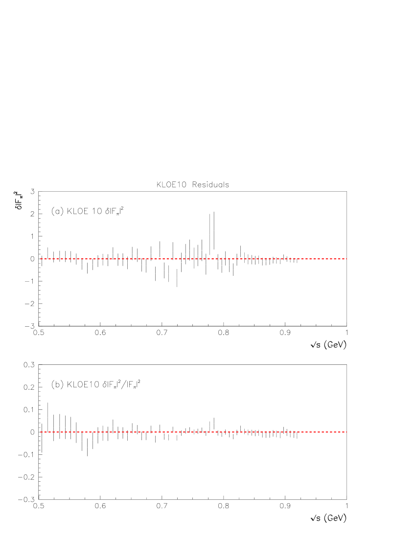
Figure 9: Fit residuals for the KLOE10 data in isolation${}^{\ref{standalone}}$. The top panel shows the function $\delta|F_{\pi}(s)|^{2}=|F_{\pi}^{KLOE10}(s)|^{2}-|F_{\pi}^{fit}(s)|^{2}$; the bottom panel displays the distribution $\delta|F_{\pi}(s)|^{2}/|F_{\pi}^{fit}(s)|^{2}$.

Similarly, the KLOE10 data set [32] returns $\chi^{2}_{KLOE10}/N_{\pi^{+}\pi^{-}}=73.68/75$ and a global fit probability of 87.7%. The fit residual distribution is shown in the top panel of Figure 9; the bottom panel in this Figure shows the fractional deviations from the fitting function. Both distributions can be considered as reasonably flat. As in the above Fig. 8, the plotted errors are the square roots of the diagonal elements of the (full) error covariance matrix. Therefore, the value for $\chi^{2}_{KLOE10}$ and the flatness of the residuals shown in Figure 9 illustrate that the (reported in [32]) full error covariance matrix looks correctly understood.

Therefore, within the global fit context, each of the NSK and KLOE10 data samples exhibits the same outstanding behavior . On the other hand, the fit parameters and error covariance matrix allows to derive, using obvious notations, $F_{\omega}^{NSK}=(1.205\pm 0.042)~{}10^{-6}$ close to the PDG value reported at top of Table 1. One also gets $F_{\omega}^{KLOE10}=(1.074\pm 0.051)~{}10^{-6}$, a $\simeq 2.5\sigma$ difference with the central value for $F_{\omega}^{NSK}$.

Under the same conditions, the (unweighted) KLOE08 data set returns $\chi^{2}_{KLOE08}/N_{\pi^{+}\pi^{-}}=96.55/60$ and a global fit probability of 56%, which is rather low. It is worth noting the remarkable flatness of the residual distributions displayed by Figure 10 which does not prevent to yield a relatively large value for $\chi^{2}_{KLOE08}$. The large $\chi^{2}_{KLOE08}$ and the flatness of the residual distribution shown in Figure 10, considered together, might indicate an issue with the non–diagonal part of the full error covariance matrix. Anyway, one can conclude that the poor KLOE08 fit probability reflects an issue with the KLOE08 error estimate rather than a distorted lineshape.

Figure 10 should be compared with the similar distribution derived formerly using a primitive version of the BHLS model (see Figure 3 in [19]). The clear improvement substantiates the gain provided by the BHLS model in its present form. On the other hand, one should also note that the value for $F_{\omega}^{KLOE08}=(1.117\pm 0.042)~{}10^{-6}$ is consistent with $F_{\omega}^{KLOE10}$.

The fit of the (unweighted) BaBar data leads to $\chi^{2}_{BaBar}/N_{\pi^{+}\pi^{-}}=343.08/270=1.27$ when limited to 1 GeV (17% probability) and to $\chi^{2}_{BaBar}/N_{\pi^{+}\pi^{-}}=340.77/275=1.24$ when going up to 1.05 GeV (corresponding to a 22% probability). The residual distribution yielded when fitting from threshold to 1.05 GeV is given in Figure 11 together with the fractional distribution. The residual distribution derived when fitting from threshold to 1 GeV, (not shown) is slightly flatter in the $\rho-\omega$ region, which indicates that accomodating simultaneously the BaBar $\omega$ and $\phi$ regions has some price. This has some consequence on the BaBar estimate of the muon anomalous moment, as will be emphasized in Subsection 6.1 below.

Nevertheless, these distributions look reasonable and are associated with quite reasonable values for $\chi^{2}_{BaBar}/N_{\pi^{+}\pi^{-}}$; the bottom panel distribution in Figure 11 is even quite similar to those derived by the BaBar Collaboration fit shown in Fig. 47 of [34] (with no quoted fit quality).

Therefore, the real issue is not the description of the BaBar spectrum stricto sensu, but its consistency with the rest of the data and physics involved in the global fit, especially the $\tau$ data. This is well reflected by the poor global fit probabilities of 17% or 22%, poorer than for the KLOE08 data sample. Qualitatively, this result could have been expected from comparing the $\tau$+PDG predictions with ”$\tau$+$(\rho-\omega)$” (using this region of the BaBar spectrum instead of the PDG information) already analyzed in Subsection 4.2.

Finally, it is worth noting that the fit outcome provides $F_{\omega}^{BaBar}=(1.628\pm 0.012)~{}10^{-6}$ (fit up to 1 GeV) or $F_{\omega}^{BaBar}=(1.575\pm 0.010)~{}10^{-6}$ (fit up to 1.05 GeV), both being far from $F_{\omega}^{NSK}$, $F_{\omega}^{KLOE08/10}$ and from PDG expectations [24].

5.1.2 Fits Combining the $e^{+}e^{-}\to\pi^{+}\pi^{-}$ Spectra

In view of the “standalone” fits just reported, we have done fits of different combinations of the scan (NSK) and ISR data samples. In this case, the contributions of the KLOE08 and BaBar samples to the (minimized) $\chi^{2}$ function are $always$ weighted as already stated.

• Combining the KLOE08 and KLOE10 data : This returns a consistent picture where $\chi^{2}_{KLOE10}$ and $\chi^{2}_{KLOE08}$ are almost unchanged compared to their “standalone” values and the fit probability reaches 81.6 %. This, indeed, confirms that they share the same physics content. This is confirmed by the fit result $F_{\omega}^{KLOE08/10}=(1.121\pm 0.038)~{}10^{-6}$, consistent with both of $F_{\omega}^{KLOE08}$ and $F_{\omega}^{KLOE10}$.

• Combining all the ISR data sets (KLOE08, KLOE10 and BaBar) : This returns $\chi^{2}_{ISR}/N_{\pi^{+}\pi^{-}}=1.34$ when including the weights for KLOE08 and BaBar and $\chi^{2}_{ISR}/N_{\pi^{+}\pi^{-}}=1.64$ when the weights are not included. The weighting used does not prevent the probability to remain poor${}^{\ref{prob_qual}}$ (1.8%) reflecting the level of inconsistency of the BaBar and KLOE(08/10) data samples already noted. In this case, one gets $F_{\omega}^{ISR}=(1.608\pm 0.010)~{}10^{-6}$, exhibiting a large distortion towards the BaBar lineshape, despite the weighting.

• Combining all $e^{+}e^{-}\to\pi^{+}\pi^{-}$ spectra : Taking the weights into account – which is more favorable – one gets $\chi^{2}_{Global}/N_{\pi^{+}\pi^{-}}=1.35$ and a fit probability${}^{\ref{prob_qual}}$ of 1.3%. Once again, the lineshape of the fit function is highly influenced by the BaBar sample in the $\rho-\omega$ interference region as shown by $F_{\omega}^{Global}=(1.582\pm 0.089)~{}10^{-6}$.

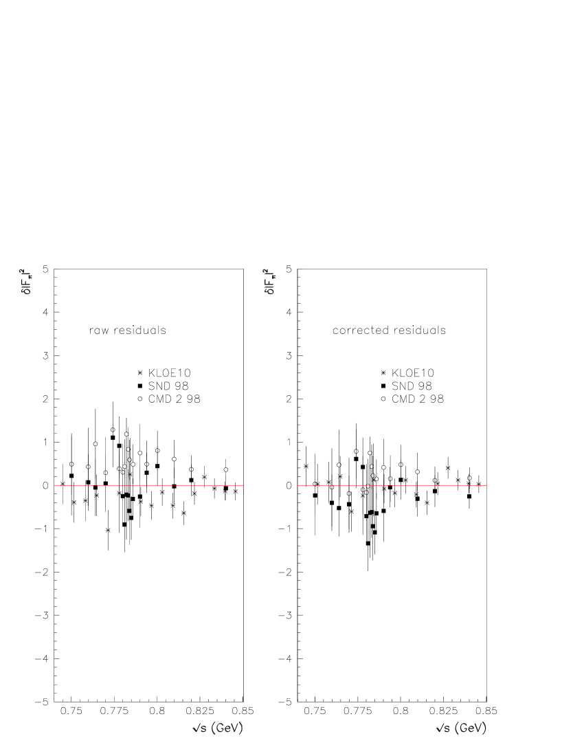
Figure 12: Fit residuals of the global fit combining NSK and KLOE10. The leftmost panel displays superimposed the residual distributions $\delta|F_{\pi}(s)|^{2}=|F_{\pi}^{EXP}(s)|^{2}-|F_{\pi}^{fit}(s)|^{2}$ for each data sample in the central energy region. The rightmost panel shows the corresponding corrected residual distributions as defined in the Appendix.

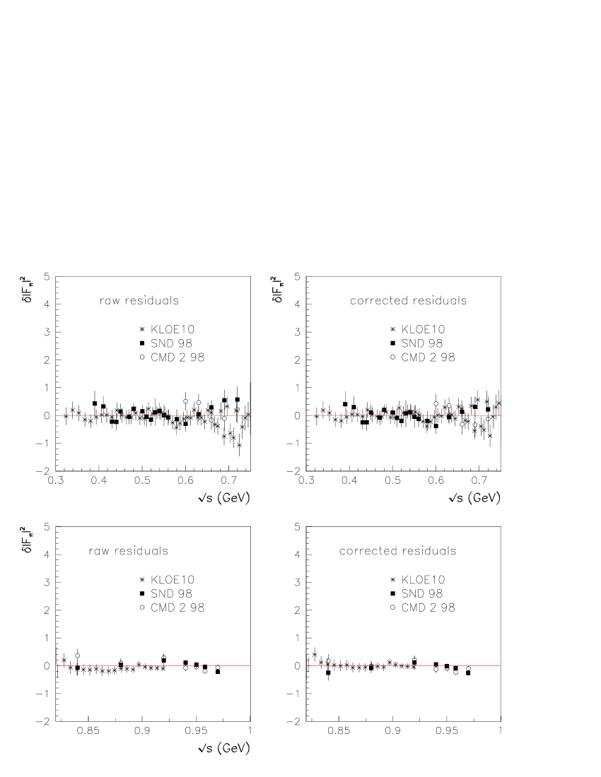
Figure 13: Fit residuals of the global fit combining NSK and KLOE10. The leftmost panels display (superimposed) the residual distributions $\delta|F_{\pi}(s)|^{2}=|F_{\pi}^{EXP}(s)|^{2}-|F_{\pi}^{fit}(s)|^{2}$ for each data sample in the side energy regions. The rightmost panels show the corresponding corrected residual distributions as defined in the Appendix.

• Combining the NSK and KLOE10 data : In this case, there is no weight and one gets $\chi^{2}_{NSK}/N_{\pi^{+}\pi^{-}}=131.37/127$ and $\chi^{2}_{KLOE10}/N_{\pi^{+}\pi^{-}}=72.90/75$ close to the “standalone”${}^{\ref{standalone}}$ fit results reported in Subsection 5.1.1 above, and thus, $\chi^{2}_{KLOE10+NSK}/N_{\pi^{+}\pi^{-}}=1.01$, and the remarkable global fit probability of 96.9 %, showing that the NSK and KLOE10 data samples are quite consistent with each other and with the rest of the BHLS physics as well. Figures 12 and 13 display the fit residuals of this common fit; in both Figures, the leftmost panels show the usual residual distributions of the NSK and KLOE10 samples (i.e. the differences between each measurement and the corresponding fitting function value), while the rightmost panels display the same information corrected for the bin–to–bin correlated uncertainties (see the Appendix).

  In both the low and medium energy regions, the data points look reasonably well distributed on both sides of the fitting function (the zero axis) and, also, the corrected residuals look closer to zero than the usual ones. If the effect of residual corrections (of pure graphical concern) looks marginal at low to medium energies, the rightmost panel of Figure 13 clearly indicates the more appropriate character of the corrected residuals to translate the fit quality.

  Data Sample	Local Probabilities (%)  (Regions in GeV)				Overall
  NSK+KLOE10	$0.30\div 0.55$	$0.55\div 0.75$	$0.75\div 0.85$	$0.85\div 1.00$	Probability
  CMD–2	$20.11$	$83.24$	$17.99$	$17.94$	20.55
  SND	$91.35$	$58.03$	$86.36$	$34.36$	92.94
  KLOE10	$99.98$	$1.69$	$30.95$	$91.11$	52.91
  Combined	$98.69$	$15.83$	$37.03$	$48.18$	57.40

  Table 2: Probabilities associated with the estimated $\chi^{2}/N_{p}$ contributions of the $\pi^{+}\pi^{-}$ data samples from CMD–2, SND and KLOE10 for the various energy regions and – last column – for each $\pi^{+}\pi^{-}$ data set. Last line is referring to what has been named NSK+KLOE10 in the text and yields a global fit probability is 96.9%; see the last paragraph in Subsection 5.1.2) for more details.

  As the global fit including simultaneously the CMD–2 [26, 27, 28], SND [29] and KLOE10 [32] $\pi^{+}\pi^{-}$ data sets play a crucial role in the present study, it looks worth to give more information on their fit quality beyond the global properties just emphasized. This is the purpose of Table 2. We choose here to present the results in terms of probabilities of the $\chi^{2}_{\pi^{+}\pi^{-}}$ contributions to the total $\chi^{2}$ associated with the corresponding number of data points $N_{\pi^{+}\pi^{-}}$. The last data column thus gives this probability for the data sample(s) provided by the three experiments. From this exercise one can conclude that the three data samples, each as a whole, behave normally with a remarquable fit quality of the SND data sample ($\chi^{2}/N_{points}\simeq 0.7$), while KLOE10 ($\chi^{2}/N_{points}\simeq 1.0$) and the (collection) of CMD–2 (($\chi^{2}/N_{points}\simeq 1.1$) data samples are quite reasonable.

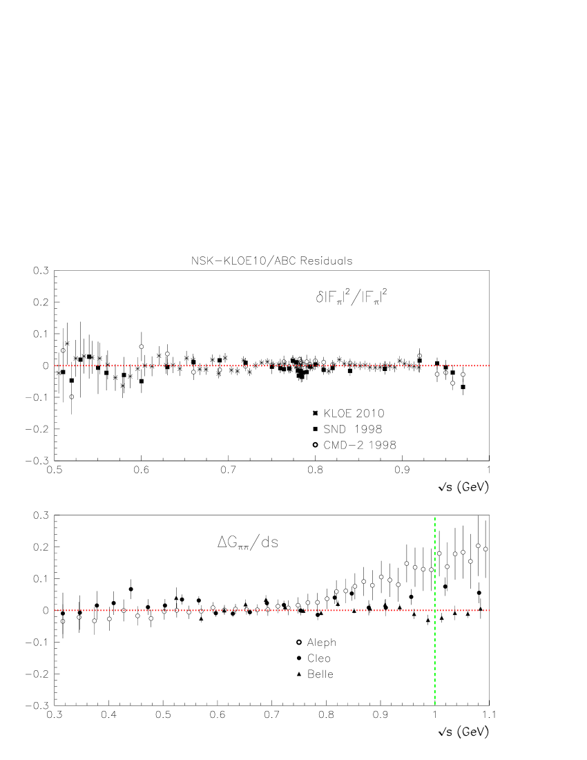
Figure 15: Fractional deviations from the fitting functions for the statistically favored configuration (NSK + KLOE10). Top panel shows the case for the pion form factor in $e^{+}e^{-}$ annihilations, bottom panel exhibits the case for the $\tau$ dipion spectra. The corrected residuals $\delta|F_{\pi}|^{2}$, as described in the Appendix, have been used for the top panel; as the spectrum in the energy region from 0.3 GeV to 0.5 GeV does not carry any interesting information, it has been removed from the Figure. The vertical line in the bottom panel indicates the end of the fitted region.

  Even if more approximate, one can perform the same exercise for various energy sub-regions. This is displayed in the first four data columns of Table 2. The probabilities of the various SND data subsamples ($N_{\pi^{+}\pi^{-}}=45)$ look reasonably flat, pointing to a very good account by the model function and one yields $\chi^{2}/N_{points}$’s ranging between 0.5 and 1.1. The probabilities of the CMD2 collection of data subsamples ($N_{\pi^{+}\pi^{-}}=82$) are less favorable (the $\chi^{2}/N_{points}$’s range between 0.7 and 1.3) but remain quite acceptable. The results for KLOE10 ($N_{\pi^{+}\pi^{-}}=75$) is more appealing as the probabilities are good for three regions (corresponding to $\chi^{2}/N_{points}$ values of resp. 0.3, 1.2 and 0.5), while the fourth region is much worse (1.7% probability corresponding to a $\chi^{2}/N_{points}$ of 1.7). This could have been already inferred by inspecting the residuals of the fit in ”isolation” shown in Figure (9). Nevertheless, Figure (15)) shows a reasonable account of the fit pion form factor even in this region.

  The last line in Table 2, which corresponds to the combination NSK+KLOE10 exhibits good probabilities up to the maximum energy and, in this case, the number of data points per energy sub–region (resp. 42, 53, 71, 36) is large enough to limit the amplitude of possible fluctuations in the $\pi^{+}\pi^{-}$ data samples.

  The global fit combining the NSK and KLOE10 data also yields

  $$F_{\omega}^{NSK+KLOE10}=(1.166\pm 0.036)~{}10^{-6}~{},$$

  which should supersede the present world average value [24] because of the full consistency it exhibits with the largest set of data ever fitted simultaneously and with a splendid probability.

5.1.3 Fits of the $e^{+}e^{-}\to\pi^{+}\pi^{-}$ Spectra : Concluding Remarks

The results reported just above have allowed us to show that the NSK data are in fair agreement with the physics represented by the $\pi^{0}\gamma$, $\eta\gamma$, $\pi^{+}\pi^{-}\pi^{0}$, $K^{+}K^{-}$, $K^{0}\overline{K}^{0}$ annihilation channels, the dipion spectra collected in the decay of the $\tau$ lepton and some more decay information listed in Subsection 3.1. This is not a really new result as this conclusion was already reached in our previous analysis [13]. The single difference with [13] is the new way to include the $\phi\to\pi^{+}\pi^{-}$ information (see Subsection 3.3), possible with the BaBar data.

The new information is that the KLOE10 data sample behaves likewise and, more importantly, that the NSK and KLOE10 data sets are consistent with each other as well as with the rest of the physics considered within the BHLS model and the global fit context.

We have performed global fits which have shown that the data from KLOE08 and BaBar have some difficulty to accommodate the global fit context. For what concerns KLOE08, the problem appears to be related with (underestimated?) systematic errors or, possibly, with their correlations. In the case of BaBar data, the problem looks more serious, as it deals with the form factor lineshape itself in the $\rho-\omega$ interference region; this issue manifests itself in the value for $F_{\omega}$, much larger than expected.

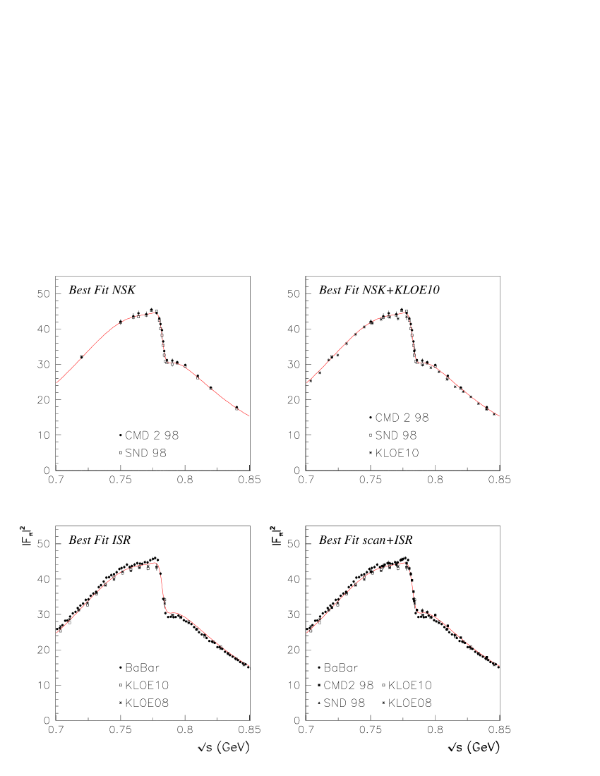
Figure 14: The Pion Form Factor in the $\rho-\omega$ region from various global fit configurations. Top left panel displays the best fit using only the CMD-2 and SND data as $e^{+}e^{-}\to\pi^{+}\pi^{-}$ spectra. Top right panel shows the case when the CMD-2, SND and KLOE10 data samples are fitted simultaneously. Bottom left panel shows the best fits when the data samples considered are those from BaBar, KLOE08 and KLOE10. Bottom right panel shows the best fit using simultaneously the CMD-2, SND, KLOE08, KLOE10 and BaBar data samples.

For this purpose, it is interesting to see the behavior of the most relevant fits of the pion form factor in the $\rho-\omega$ resonance region. These are displayed in Figure 14. The best fit obtained using only the NSK data is shown in the top left panel and is clearly quite satisfactory. The top right panel exhibits the case when the NSK data are complemented with the KLOE10 sample; this fit is also quite successful.

Bottom left panel in Figure 14 shows the behavior of the best fit function when only considering the ISR data (BaBar, KLOE08, KLOE10) and bottom right panel when taking into account all existing scan and ISR data. Both are clearly less satisfactory reflecting mostly the tension between BaBar and the KLOE data sets.

As already stated, the largest favored configuration is to include simultaneously the NSK and KLOE10 samples within the fit procedure. Fig. 15 shows the fractional deviations from the fitting functions for the $e^{+}e^{-}$ and $\tau$ data derived simultaneously from the global fit. The top panel is clearly consistent with a flat distribution. The bottom panel shows that CLEO and Belle distributions are flat, but also that ALEPH data may show a slight $s$–dependence starting around 0.8 GeV (quite similar to the top panel in Fig. 55 from [34] or to Fig.12 in [23]). This is a pure consequence of having introduced the KLOE10 data sample.

One may thus consider that the statistically favored configurations (the so–called NSK and NSK+KLOE10 global fit configurations) exhibit flat residual distributions simultaneously in $e^{+}e^{-}$ and $\tau$ $\pi\pi$ channels.

The question is now whether the KLOE08 and BaBar data samples can nevertheless help to improve some physics information of important concern as the muon $g-2$. This will be discussed in the forthcoming Section. Anyway, the KLOE10 data sample already allows to confirm the results already derived using the NSK data and, even, helps in getting improved results.

5.2 Physics Information Derived From Global Fits

5.2.1 The $\phi$ Region in the $e^{+}e^{-}\to\pi^{+}\pi^{-}$ Spectrum

Up to now, the $\phi$ pieces of information used in our fits/predictions are the RPP value for the product $F_{\phi}={\rm Br}(\phi\to e^{+}e^{-}){\rm Br}(\phi\to\pi^{+}\pi^{-})=(2.2\pm 0.4)~{}10^{-8}$ and the ”Orsay” phase for the $\phi\to\pi^{+}\pi^{-}$ amplitude provided by SND [72], namely $-34.0\pm 4.0$ degrees. In order to avoid over interpreting the SND phase as an Orsay phase (i.e. identified with the phase of the product $F_{\omega\phi}^{e}(s)~{}g_{\phi\pi\pi}(s)$ in Eq. (14) at $s=m_{\phi}^{2}$), we have found worth revisiting this assumption. Using the NSK and KLOE10 data sets as reference $\pi^{+}\pi^{-}$ data sample, we have performed several global fits within the BHLS framework.

For definiteness, and for an easy comparison, the first line in Table 3 displays the values extracted from [24, 72] and used in all fits referred to up to now. The second line in this Table displays the corresponding values reconstructed using the final parameter values from the appropriate global fit. The goodness of fit (94.5% probability) is reflected by the $\chi^{2}$ values shown in the last two data columns. The reconstructed value for $F_{\phi}$ is in very good accord with the (input) RPP value, while the phase is shifted toward slightly more negative values than the SND datum.

The fit results summarized in the third line are obtained by withdrawing the SND phase [72] from the minimization procedure. The fit quality is almost unchanged (95.3% probability) and the expected $F_{\phi}$ is still well reproduced; on the other hand, the $\phi$ phase moves by about $3\sigma$ but remains significantly negative.

In both cases, the pion form factor lineshape exhibits the behavior shown in Figure (1b), e.g. a tiny peak at the $\phi$ mass, resembling what is shown in Figure 4 of [72].

The next step has been to remove the reference values for $F_{\phi}$ and for the $\phi$ phase and supplement the NSK and KLOE10 data with the $\phi$ region spectrum from BaBar data ($\sqrt{s}\in[1.00,1.05]$ GeV). The important results are shown in the fourth line of Table 3. The fit probability remains good (91.3%), but the $\chi^{2}$ of the NSK+KLOE10 data is degraded by $\simeq 10$ units, which may indicate some tension between these data sets and the coherent background beneath the $\phi$ peak. The fit value for $F_{\phi}$ increases by 50% but remains perfectly consistent with expectations [24]. In contrast, the Orsay phase changes dramatically (from $-[30\div 50]^{\circ}\to 150^{\circ}$). The lineshape exhibited by the BaBar pion form factor is almost identical to those shown in Figure (1c).

$\phi$ Information Used	$F_{\phi}\,10^{8}$	Orsay Phase	$[\chi^{2}_{\pi^{+}\pi^{-}}/N_{points}]_{<1.0~{}GeV}$	$[\chi^{2}_{\pi^{+}\pi^{-}}/N_{points}]_{\phi}$
Input [24, 72]	$2.2\pm 0.4$	-$34.0\pm 4.0$	-	-
Imposing Orsay phase [72]	$2.34\pm 0.42$	-$41.45\pm 1.89$	$204.3/202$	$2.25/2$
Releasing Orsay phase	$2.23\pm 0.41$	-$48.23\pm 1.88$	$202.9/202$	$0.04/1$
BaBar $\phi$ Region Spectrum [33]	$3.31\pm 0.99$	$156.92\pm 2.76$	$215.0/202$	$5.2/5$
BaBar data [33] fit	$3.04\pm 0.60$	$153.41\pm 0.98$	$(338.1/270)$	$(2.69/5)$
Imposing BaBar $\phi$ parameters	$3.05\pm 0.50$	$153.37\pm 0.85$	$208.0/202$	$0.05/2$

Table 3: Fit results for $F_{\phi}={\rm Br}(\phi\to e^{+}e^{-}){\rm Br}(\phi\to\pi^{+}\pi^{-})$ and for the ”Orsay” phase (in degrees) for the $\phi$ amplitude. See Subsection 5.2.1 for comments.

As stated above${}^{\ref{bbr_phi}}$, the $[1.00,1.05]$ GeV region of the BaBar spectrum carries information on the $\phi$ signal but also on the underlying ($\rho$ coherent) background. In order to substantiate its effect, we have finally performed a fit using as input the $F_{\phi}$ and $\phi$ phase values extracted from fitting the BaBar data up to 1.05 GeV (see Subsection 5.1.1); the corresponding values are given in the fifth data line of Table 3 and, when imposed to the fit procedure, these numbers lead to the results shown in the last line. The fit probability improves to 94%.

As a summary, Table 3 shows that some ambiguity occurs about the pion form factor behavior in the $\phi$ region. It becomes interesting to have new data covering this region, in order to decide which among Figures (1b) and (1c) reflects the right behavior. It is also interesting to examine the consequences of this ambiguity on $g-2$ estimates.

Without going into details (addressed in the next Section), we can give the values for $\Delta a_{\mu}=a_{\mu}^{exp}-a_{\mu}^{th}$ corresponding to the various cases shown in Table 3. In units of $10^{-10}$, the values for $\Delta a_{\mu}$ are respectively $39.91\pm 5.21$ (line # 2), $39.35\pm 5.23$ (line # 3), $37.18\pm 5.16$ (line # 4) and $39.32\pm 5.20$ (line # 6). The most likely effect this implies on $\Delta a_{\mu}$ is a possible $shift$ by $0.59\times 10^{-10}$ (lines # 2, 3, 6). A maximum possible shift is $2.73\times 10^{-10}$ (lines # 2 and 4). Instead, the uncertainty is practically unchanged. Taking into account the uncertainty on $a_{\mu}^{exp}$ [39, 40], the effect of this shift on the significance of $\Delta a_{\mu}$ is quite marginal ($4.88\sigma\rightarrow 4.57\sigma$). Nevertheless, this shift plays as a systematic effect to be accounted for in the final value which will be proposed for $a_{\mu}^{th}$.

5.2.2 The HLS Favored Solution : Fit Parameters and Physics Quantities

In our previous analysis [13], we encountered some tension in the $e^{+}e^{-}$ annihilation data in the $\phi$ region between the $e^{+}e^{-}\to\pi^{+}\pi^{-}\pi^{0}$ channel and the $e^{+}e^{-}\to K^{+}K^{-},K^{0}\overline{K^{0}}$ channels. Including all data in the global fit defined what we called ”configuration A”. Alternatively, we excluded the 3-pion data in the vicinity of the $\phi$ mass from the fit. In this case, the corresponding collection of data included in the fit was called ”configuration B”, which yields a better fit probability. As [13], the present analysis privileges configuration B as a basis. However, as the ”observed” tension could not be abnormal, we also consider fits based on configuration A for completeness, essentially in relation with the muon anomalous moment.

Tables 4 and 5 display the global fit parameter values within configuration B, using the $e^{+}e^{-}$ data from only CMD–2, SND and KLOE10. This corresponds to the so–called NSK+KLOE10 case which is favored by the BHLS model and breaking scheme.

The top part of Table 4 displays information directly related with the standard parameters of the original HLS model. The value for $a$ is found, as usual [18] significantly larger than the standard VMD expectation ($a=2$) and the value for the universal vector coupling $g$ stays at accepted values [7]. The HLS parameters giving the weight of the anomalous terms [55, 15] in the global HLS model $(c_{3}+c_{4})/2$, $c_{1}-c_{2}$, get values close to our previous results [13]. The parameter $v$, related with the ’t Hooft determinant terms [54], will be discussed below.

The middle part of Table 4 essentially displays the SU(3) breaking parameters generated by the original BKY mechanism [16]; their role is crucial in the $e^{+}e^{-}\to K\overline{K}$ cross sections and in the $VP\gamma$ couplings (see Appendix E in [13]). The values for $z_{A}$, $z_{V}$ and $z_{T}$ show that the breaking of the SU(3) symmetry generates departures from 1 (unbroken case) by 30% to 60%.

The bottom part of Table 4 shows specifically the values for the BKY parameters generating the (direct) isospin breaking mechanism [53, 13] defined in Subsection 2.2 : $\Delta_{V}$, $\Delta_{A}$ and $\Sigma_{V}$ which vanish when Isospin Symmetry is not broken. Numerically, they are at the level of a few percents, i.e. much smaller than those corresponding to the breaking of the SU(3) symmetry, as expected. The value for $g_{\omega\to\pi\pi}^{direct}$ which only depends only on the direct IB breaking mechanism is discussed just below.

The fit results shown in Table 5 deal with the subtraction polynomials coming with the various loops (see Section 6 in [13] or, more deeply, Section 12 in [18] and especially Table 3 therein). The bottom part of Table 5 gives the subtraction polynomials of the functions $\varepsilon_{1}(s)$ and $\varepsilon_{2}(s)$ which define the vector meson mixing as reminded in Subsection 2.3. They are given for sake of completeness as, generally, they do not carry an obvious intuitive meaning; they mostly play a role in the definition of the vector meson mixing [13]. Nevertheless, as clear from Eqs. 9, via the mixing angles $\alpha(s)$ and $\beta(s)$, the functions $\varepsilon_{1}(s)$ and $\varepsilon_{2}(s)$ play a fundamental role in reconstructing $F_{\omega}$ and $F_{\phi}$ discussed at several places above and they have been shown to produce the expected effect either isolatedly ($F_{\phi}$ only depends on vector meson mixing) or combined with the direct IB [53, 13] discussed above ($F_{\omega}$ depends on both).

Table 6 display physics parameters which can be compared with corresponding information derived by others : different theoretical frameworks or measured quantities not included in our fit procedure; this may give confidence in the validity of the BHLS model and its structure.

If the universal coupling $g$ is indeed returned by fits at usual values, the reconstructed value for $g_{\rho\pi\pi}$ compares reasonably well with its value derived from fits using the Gounaris–Sakurai parametrization [7] $g_{\rho\pi\pi}=6.1559$.

In their mini-review [24], Rosner and Stone conclude that the most likely estimate for $f_{K}/f_{\pi}$ can be summarized by $f_{K}/f_{\pi}=1.197\pm 0.002_{exp}\pm 0.002_{CKM}\pm 0.001_{rad.~{}cor.}$ which compares reasonably well with our own estimate reported in Table 6. This also indicates that this proposed value could be included in our fit procedure as an additional constraint.

The following datum is our estimate for $g_{\omega\to\pi\pi}^{direct}$. A piece of information recently studied in [71] is related with the ratio $G=g_{\omega\to\pi\pi}^{direct}/g_{\rho\pi\pi}$. Our previous estimate [13], using only the CMD–2 and SND data within our global framework, was $(3.47\pm 0.64)\%$ smaller than the findings of [71]; from Table 6, this ratio is now estimated at $(6.27\pm 0.94)\%$, just in between the two estimates proposed by Maltman and Wolfe [71], showing the influence of the KLOE10 data.

Our estimate for the ’t Hooft parameter $\lambda$ [54], which governs the magnitude of nonet symmetry breaking in the pseudoscalar sector (cf. Eq. (7) in [13]), can be derived from the values for $v$ and $z_{A}$ (cf. Eq. (22) in [13]). We confirm that $\lambda$ is in the range of $10\%$ with a substantial uncertainty (30%); we are not aware of published external estimate of this quantity.

The following part of Table 6 deals with information concerning mixing properties in the pseudoscalar sector. We have adopted as parametrization of the $\pi^{0}-\eta-\eta^{\prime}$ mixing those proposed in [75]. Within this parametrization, the $\pi^{0}-\eta$ mixing is governed by $\epsilon$, the $\pi^{0}-\eta^{\prime}$ mixing is governed by $\epsilon^{\prime}$. Both parameters are expected to carry values at the few percent level, and one may expect $\epsilon^{\prime}<\epsilon$. These expectations are satisfied by our estimates. Moreover, $\epsilon$ and $\epsilon^{\prime}$ can be expressed [13] in terms of the pseudoscalar singlet–octet mixing angle $\theta_{PS}$ and of some $\epsilon_{0}$, function of the quark masses [75]. Recent estimates yield $\epsilon_{0}=(1.31\pm 0.24)\%$ [76] and $\epsilon_{0}=(1.16\pm 0.13)\%$ [77], significantly smaller than our former result ($\epsilon_{0}=(3.16\pm 0.23)\%$). Our present evaluation (see Table 4), is much closer to these expectations.

The pseudoscalar mixing angles are not basic parameters in our fit procedure but depend on $\lambda$ and $z_{A}$ already discussed (cf. Eqs. (26) in [13]). An early study [78] concluded that the mixing angle $\theta_{0}$ defined in the mixing scheme developed in [49, 50] was consistent with zero. This has been confirmed in [13] ($\theta_{0}=-1.11^{\circ}\pm 0.39^{\circ}$); quite recently, Chen et al. [79] yield $\theta_{0}=(-2.5\pm 8.2)^{\circ}$ from a study of radiative decays. This motivates imposing the condition $\theta_{0}\equiv 0$ to our fit procedure. From the expressions for $\theta_{8}$ and $\theta_{PS}$ (in terms of $z_{A}$ and $\lambda$, or, equivalently, $v$), we derive $\theta_{8}=-24.61^{\circ}\pm 0.21^{\circ}$, quite consistent with the recent $\theta_{8}=-21.1^{\circ}\pm 6.0^{\circ}$ [79] and much more precise.

Our evaluations of $\theta_{PS}=-13.54^{\circ}\pm 0.15^{\circ}$ compares favorably with its KLOE measurement [80] ($-13.3^{\circ}\pm 0.3_{stat}^{\circ}\pm 0.7_{syst}^{\circ}\pm 0.6_{th}^{\circ}$), recently confirmed by GAMS ($-13.4^{\circ}\pm 1.8^{\circ}$).

To end up with this topic, we should mention that the fit values for the partial widths $\pi^{0}\gamma\gamma$, $\eta\gamma\gamma$ and $\eta^{\prime}\gamma\gamma$ are at resp. $0.3\sigma$, $0.5\sigma$ and $0.2\sigma$ from RPP expectations [24].

Our evaluation for the $\omega$ and $\phi$ mass and width are also shown in Table 6. These correspond to the usual definition of the inverse propagator with fixed width :

$$D_{V}^{-1}(s)=s-m_{V}^{2}+im_{V}\Gamma_{V}\;.$$ (17)

They are found in fair consistency with RPP expectations and our global fit estimates compare favorably with the corresponding data extracted from fits to the individual measured annihilation spectra reported in [24].

The last line in Table 6 displays information on the $\rho$ meson mass and width. Concerning objects as broad as the $\rho$ meson, mass and width values are highly definition–dependent [18] and, depending upon the choice, their spread can easily amount to about 20%. In Table 6, we give the location $s_{\rho}$ of the $\rho^{0}$ propagator pole located in the unphysical sheet; it has been derived using the parameter values and their error covariance matrix within a Mathematica code. Defining $s_{\rho}=M_{\rho}^{2}-iM_{\rho}\Gamma_{\rho}$, one can derive mass and width values, also given in Table 6. As far as we know, one can only compare with [81] (see also [82] for a hint on the parametrization dependence of the pole location), who performed fits by approximating the $\rho$ propagator by a Laurent series; this Reference reports $M_{\rho}=757.5\pm 1.5$ MeV and $\Gamma=142.5\pm 3.5$ MeV relying on fitting only the data reported in [25], close to our results. The previous estimate of these within the HLS model [18] where larger (resp. 760.4 and 144.6) with comparable uncertainties; however, the data from Belle and KLOE were not available at that time. Because of our approximations (see Subsection 2.6), the present study is not sensitive to differences between the charged and the neutral $\rho$ mesons.

$g$ (HLS)	$a$ (HLS)	$(c_{3}+c_{4})/2$	$c_{1}-c_{2}$	$v$
$5.578\pm 0.001$	$2.398\pm 0.001$	$0.920\pm 0.004$	$1.226\pm 0.026$	$0.030\pm 0.012$
$z_{A}$	$z_{V}$	$z_{T}$	$\epsilon_{0}$	–
$1.608\pm 0.006$	$1.319\pm 0.001$	$1.409\pm 0.062$	$0.026\pm 0.003$	–
$\Delta_{A}$	$\Sigma_{A}$	$\Delta_{V}$	$\Sigma_{V}$	$h_{V}$
$0.048\pm 0.007$	0	$-0.028\pm 0.003$	$-0.034\pm 0.001$	$2.853\pm 0.291$

Table 4: Parameter values from the global fit using the CMD–2, SND and KLOE10 data. The piece of information written boldface was not allowed to vary within the fit procedure.

Parameter	Sub. Pol. $\Pi_{\pi\pi}^{\rho}(s)$	Sub. Pol. $\Pi_{\pi\pi}^{W/\gamma}(s)$
$C_{1}$ (GeV-2)	0	$0.671\pm 0.041$
$C_{2}$	$-0.473\pm 0.001$	$0.730\pm 0.063$
	Sub. Pol. $\varepsilon_{2}(s)$	Sub. Pol. $\varepsilon_{1}(s)$
$C_{1}$ (GeV-2)	$-0.075\pm 0.006$	$-0.015\pm 0.002$
$C_{2}$	$0.034\pm 0.005$	$0.015\pm 0.002$

Table 5: Parameter values from the global fit using the CMD–2, SND and KLOE10 data (cont’d). The boldface parameter is not allowed to vary. Each subtraction polynomial is supposed to be written in the form $C_{1}s+C_{2}s^{2}$. The functions $\varepsilon_{1}(s)$ and $\varepsilon_{2}(s)$ are combinations of the kaon loops which govern the neutral vector meson mixing (see Subsections 2.3 and 5.2.2).

$g_{\rho\pi\pi}$	$f_{K}/f_{\pi}$	$g_{\omega\to\pi\pi}^{direct}$	$\lambda$
$6.505\pm 0.003$	$1.279\pm 0.010$	$0.408\pm 0.061$	$(7.64\pm 3.19)~{}10^{-2}$
$\epsilon$	$\epsilon^{\prime}$	$\theta_{8}$ (deg)	$\theta_{PS}$ (deg)
$(4.027\pm 0.474)~{}10^{-2}$	$(0.975\pm 0.122)~{}10^{-2}$	$(-24.61\pm 0.21)^{\circ}$	$(-13.54\pm 0.15)^{\circ}$
$m_{\omega}$ (MeV)	$\Gamma_{\omega}$ (MeV)	$m_{\phi}$ (MeV)	$\Gamma_{\phi}$ (MeV)
$782.52\pm 0.03$	$8.66\pm 0.04$	$1019.25\pm 0.26$	$4.18\pm 0.02$
$m_{\rho}$ (MeV)	$\Gamma_{\rho}$ (MeV)	${\cal R}e(s_{\rho})$ (GeV2)	${\cal I}m(s_{\rho})$ (GeV2)
$753.8\pm 0.5$	$138.10\pm 0.5$	$0.5682\pm 0.0007$	$0.1041\pm 0.0004$

Table 6: Physics parameters extracted from the BHLS favored fit.

6 Hadronic Contribution to the Muon $g-2$ Estimates

In order to estimate the hadronic contribution to the muon anomalous magnetic moment $a_{\mu}$, the method followed in the present work is identical to the one used in [13]. In this Section, we examine the global fit solutions provided by the data samples listed in Subsection 3.1; the various cases correspond to varying the $e^{+}e^{-}\to\pi^{+}\pi^{-}$ data sample combination submitted to the global fit procedure. We mostly work under the configuration B which has been reminded in the header of Subsection 5.2.2 just above.

6.1 $a_{\mu}(\pi\pi)$ Contribution from the Reference $m_{\pi\pi}$ Region

In order to emphasize what is going on, it is worth examining the contribution to $a_{\mu}(\pi\pi)$ provided by the invariant mass interval ${\cal A}\equiv\left[0.630,~{}0.958\right]$ GeV. As for this reference region, all experimental groups have published the numerical integration leading to their estimate of $a_{\mu}(\pi\pi,\cal{A})$ (using Eq. (1) with the experimental spectra), one can compare our fit outcome with these. When combining data sets within the fit procedure, we compare to the usual weighted average of the $a_{\mu}(\pi\pi,\cal{A})$ values provided by each experimental group.

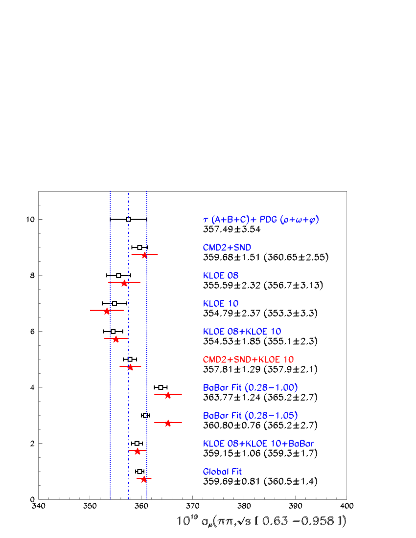
Figure 16: The muon anomalous magnetic moment. The numbers gives the $\pi\pi$ contribution from the $(0.630,~{}0.958)$ GeV invariant mass region. The results from fits are shown with empty squares, the experimental estimates by stars. Fit values are given followed by the experimental estimate within brackets. Global fit properties favor the result from the CMD2+SND+KLOE10 combined sample.

The results for $a_{\mu}(\pi\pi,\cal{A})$ are collected in Fig. 16 and will be discussed from top to bottom. The first point has no experimental partner, as it comes out from the $\tau$+PDG fit described in Section 4. The dashed–dotted line is drawn through the central value of this prediction, the dotted lines show the corresponding $\pm 1\sigma$ band.

It should then be noted that most experimental estimates happen to be inside the $1\sigma$ band of the $\tau$+PDG prediction. KLOE10 is at the border, while BaBar is rather larger by about $2\sigma$. One should also note that KLOE08 as well as the combination CMD2+SND+KLOE10 (our preferred combination because of its global fit properties) provide central values which coincide almost exactly with the $\tau$+PDG expectation; even if shifting the $\tau$+PDG prediction by $(1\div 2)~{}10^{-10}$ should be performed (see Subsection 6.4.1 below), the overall agreement remains noticeable. This looks to us an important property taking into account the long–standing discussion about the $\tau-e^{+}e^{-}$ issue. Our results tend to prove that this issue vanishes once the breaking mechanism is appropriate.

The next point shows the global fit estimate (square symbol) while using${}^{\ref{standalone}}$ “solely” the NSK data (especially those from [27, 28, 29], but also those from [25, 26]). The present fit value is found smaller than those published in [13] by about $1\times 10^{-10}$. This shows that the effect of our updating the $\phi$ data decay information extends over the whole spectrum. The uncertainty is unchanged and amounts to a 40% gain compared with the experimental estimate. This gain is a pure effect of the global fit procedure where the channels others than $\pi^{+}\pi^{-}$ allow to improve $also$ the $\pi^{+}\pi^{-}$ contribution importantly because of the underlying VMD physics correlations.

The following point is derived using${}^{\ref{standalone}}$ “solely” the KLOE08 data sample. As while fitting “solely” the NSK data, the fit outcome also differs by $1\times 10^{-10}$ from the experimental central value. The fit result associated with the KLOE10 data sample is also found in good agreement with the experimental expectation and one should note that both differ by $1.5\times 10^{-10}$ in opposite directions. In contrast, the fit result for the mixed KLOE10+(weighted) KLOE08 data sample is found to agree very well with expectation (a $0.6\times 10^{-10}$ difference only).

The data point associated with the CMD2+SND+KLOE10 combined data sample is found in much better accord with the average of the experimental data; in this case, the error is also improved by about a factor 2 compared with the experimental value, but, interestingly, first, the central reconstructed value does not exhibit any significant systematic shift ($\simeq 0.1\times 10^{-10}$) compared to the experimental expectation, second, the central reconstructed value is in perfect accord with the $\tau$+PDG prediction, as already noted.

The next pair of points shows the case for the BaBar data. While using the whole spectrum up to 1 GeV, the fitting function provides an estimate for $a_{\mu}(\pi\pi,\cal{A})$ in good agreement with the expected experimentally integrated value. However, extending the fitting region up to 1.05 GeV, increases the difference between the fit outcome and the experimental expectation from $1.5\times 10^{-10}$ to $4.4\times 10^{-10}$, which illustrates some issue in the $\omega$ region when also fitting the BaBar $\phi$ region.

The last two points (ISR and scan + ISR data, resp.) correspond to fitting the whole spectra up to 1 GeV while weighting the KLOE08 and BaBar contributions to the $\chi^{2}$. The results look in good correspondence with the weighted averages of the direct integration results, and one remains within the $1\sigma$ band of the $\tau$+PDG expectation.

The contribution to $a_{\mu}(\pi\pi)$ from the invariant mass interval ${\cal A}\equiv\left[0.630,~{}0.958\right]$ GeV and the global fit properties (see Section 5) allow to draw a few important conclusions :

• (l) There is no mismatch between the $\tau$+PDG expectations and the estimates derived from the fitting functions or those derived from the numerical integration of the measured $e^{+}e^{-}\to\pi^{+}\pi^{-}$ cross sections. To be more precise, when some departure is observed, it is always closely associated with poor global fit qualities of the corresponding data sample.

• (ll) One can take as reference $e^{+}e^{-}\to\pi^{+}\pi^{-}$ data the NSK (CMD-2 & SND) $and$ KLOE10 data samples. Separately and together, they are found in perfect accord with all annihilation data considered ($\pi^{0}\gamma$, $\eta\gamma$, $\pi^{+}\pi^{-}\pi^{0}$, $K^{+}K^{-}$, $K^{0}\overline{K}^{0}$ final states) as well as with the published dipion spectra in the decay of the $\tau$ lepton and the few additional decay information introduced within the global fit BHLS framework. The uncertainty is improved by a factor of about 2.

• (lll) Comparing the central value for $a_{\mu}(\pi\pi,\cal{A})$ derived from the fitting function – using the NSK and KLOE10 data samples within the global framework – with its direct estimate indicates that the estimate derived from the fit is almost unbiased ($\simeq 0.1\times 10^{-10}$). In contrast, the fitting functions derived from the fits to each of the NSK and KLOE10 data separately may exhibit a small bias (a shift of $\simeq 1\times 10^{-10}$).

• (lv) One may remark that the global fit using all existing $e^{+}e^{-}\to\pi^{+}\pi^{-}$ scan & ISR data also provides reasonable values for $a_{\mu}(\pi\pi,\cal{A})$ without a significant bias and with a much improved uncertainty. This reduced uncertainty may look too optimistic, taking into account the global fits properties of the corresponding sample combinations. Nevertheless, one may note that the last two entries in Fig. 16, derived by weighting the KLOE08 and BaBar samples with respect to all others, do not depart from the general trend.

6.2 The Full Muon Anomalous Magnetic Moment $a_{\mu}$

Here we are interested in the theoretical prediction of the muon anomalous magnetic moment and its comparison with the experimental result [39, 40]. Our BHLS based global fit results provides the dominant contribution to the hadronic vacuum polarization contribution.

Several global fits have been performed using different groups of $e^{+}e^{-}\to\pi^{+}\pi^{-}$ data samples. The resulting fitting functions and the parameter error covariance matrices have allowed to derive the leading order hadronic contribution (LO–HVP) to $a_{\mu}$ up to 1.05 GeV in various cases. The full HVP is obtained by combining our present results with the other hadronic contributions listed in Table 9 of our previous work [13]. The various evaluations of the muon $g-2$ are calculated by summing up $a_{\mu}^{LO-HVP}$ with the Higher order HVP, the QED and electroweak (EW) contributions and the so–called light–by–light (LBL) contribution; for this purpose, the values given in Table 10 of [13] have been updated (see Table 7 below).

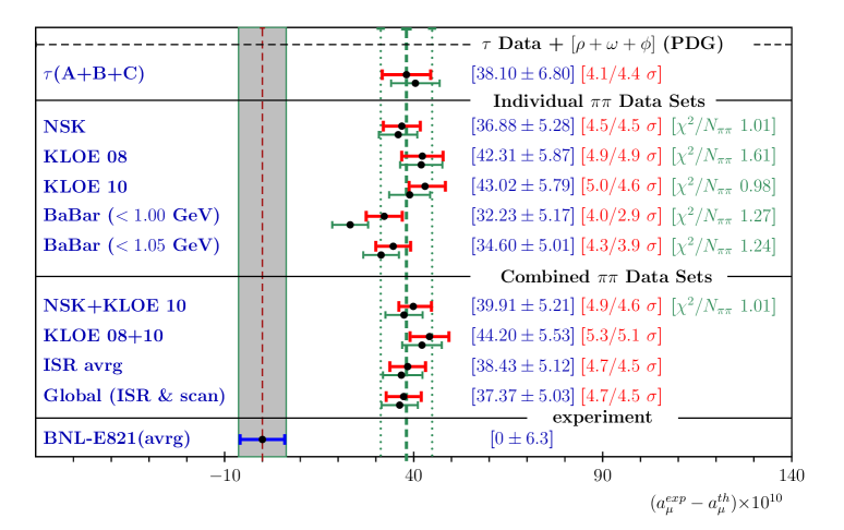
Figure 17: The deviation $\Delta a_{\mu}\times 10^{10}$ between experiment and theory for the anomalous magnetic moment of the muon. The leading hadronic vacuum polarization contribution has been estimated via global BHLS model fits for different $e^{+}e^{-}\to\pi^{+}\pi^{-}$ data samples.The $\tau$ predictions – using or not the spacelike data – are given in the top pair lines, followed by the fit results using each scan or ISR data sample in isolation or combined; see text for comments.

In Figure 17, we display results for the deviation $\Delta a_{\mu}=a_{\mu}^{\rm exp}-a_{\mu}^{\rm th}$ between experiment and theoretical predictions in units of $10^{-10}$, for various fit results which only differ by the indicated $e^{+}e^{-}\to\pi^{+}\pi^{-}$ data sample considered within the fit procedure.

Specifically, the fit results included in Fig. 17 are all based on the “configuration B” data set introduced in [13]. Furthermore, always included in the fits are all channels listed in Subsection 3.1, especially the $\tau$ data.

At top of the Figure, we provide the $\tau$+PDG entry (i.e., without using any $e^{+}e^{-}\to\pi^{+}\pi^{-}$ data set in the fit procedure). The twin points drawn correspond to $\Delta a_{\mu}=a_{\mu}^{exp}-a_{\mu}^{th}$ in units of $10^{-10}$; the lower point is obtained using the spacelike data [35, 36], the upper one by excluding them from the fit. The number following the point is the estimate for $\Delta a_{\mu}$ from fits excluding the spacelike data. The significance of this difference is written [$x/y~{}\sigma$], $x\sigma$ being the significance obtained when excluding the spacelike data, $y\sigma$ when they are included into the fit procedure. The last column in this Figure provides the $\chi^{2}/n_{points}$ for the $e^{+}e^{-}\to\pi^{+}\pi^{-}$ data; this number is given only for (combination of) samples used without any weight.

The first remark which can be drawn is that including the spacelike data does not change noticeably the value for $\Delta a_{\mu}$ nor its statistical significance. The second important point is that all the features noted while discussing $a_{\mu}(\pi\pi,\left[0.630,~{}0.958\right]~{}{\rm GeV})$ in the previous Subsection survive when dealing with the whole provided spectra (see (l)–(lv) just above).

It was noted in [13] that the use of the ISR data should not dramatically improve the uncertainty of the theoretical estimate : going from scan data only (the NSK entry) to scan+ISR data (the ”Global Fit” entry) improves the uncertainty by only $0.3\times 10^{-10}$; this is the major gain of working in a global fit context [13]. In contrast, the central value exhibits slightly more sensitivity, as can be seen by comparing the various entries.

Anyway, the present analysis allows to conclude that the discrepancy between the measurement for $a_{\mu}$ [39, 40] and the Standard Model prediction is certainly in the range of $4.5\sigma$ or slightly higher. Taking into account the already reported fit qualities, the most favored value for $a_{\mu}^{LO-HVP}$ is :

$$a_{\mu}^{LO-HVP}=(681.23\pm 4.51)~{}10^{-10}.$$ (18)

This value is derived by introducing the $e^{+}e^{-}$ NSK and KLOE10 data samples within our global fit procedure; systematics on this number will be discussed with the final result (Subsection 6.4).

Finally, we have redone several of our fits within the configuration A. These confirm the results derived within the configuration B which are the body of the present paper. One also confirms the ’tension’ reported in [13] between the 3–pion spectra in the $\phi$ region and the data collected for both $e^{+}e^{-}\to K\overline{K}$ cross sections. Whether this is an experimental issue, or if this indicates that our breaking model should be extended is an open issue. Nevertheless, some physics results derived within the configuration A will be presented just below for completeness.

6.3 Comparison with Other Estimates of $a_{\mu}$

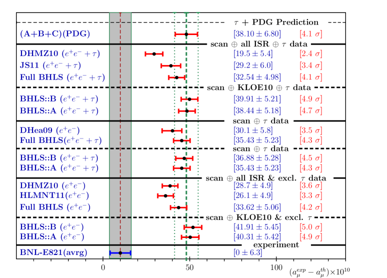
Figure 18: A set of recent estimates of the muon anomalous magnetic moment deviation from the BNL average value [39, 40]. Our own (updated) estimates are figured by BHLS::A and BHLS::B for respectively configurations A and B. The results obtained using $all$ the ISR data samples inside the global fit procedure are displayed under the tag Full BHLS. The statistical significance of each $\Delta a_{\mu}$ is displayed on the right hand side of the Figure. See the text for more information.

Fig. 18 reports on some recent estimates of the muon anomalous magnetic moment $a_{\mu}$ together with the BNL average value [39, 40]. In this Figure, our (favored) results – derived using only the CMD–2, SND and KLOE10 data samples – are given under the entry tags BHLS::A (for configuration A) and BHLS::B (for configuration B). Some evaluations proposed by other authors are also shown; they are extracted from [6] (DHMZ10), [7] (JS11), [8] (DHea09) and [9] (HLMNT11).

$10^{10}a_{\mu}$	Values (incl. $\tau$)		Values (excl. $\tau$)
	scan only	scan $\oplus$ ISR	scan $\oplus$ ISR	scan only
LO hadronic	$685.66\pm 4.54$	$688.60\pm 4.24$	$687.53\pm 4.34$	$684.25\pm 5.15$
HO hadronic	$-9.97\pm 0.09$
LBL	$10.5\pm 2.6$
QED	$11~{}658~{}471.8851\pm 0.0036$
EW	$15.40\pm 0.10_{\rm had}\pm 0.03_{\rm Higgs,top,3-loop}$
Total Theor.	$11~{}659~{}173.48\pm 5.23$	$11~{}659~{}176.42\pm 4.89$	$11~{}659~{}175.35\pm 5.06$	$11~{}659~{}171.89\pm 5.77$
Exper. Aver.	$11~{}659~{}208.9\pm 6.3$
$\Delta a_{\mu}$	$35.43\pm 8.14$	$32.48\pm 8.03$	$33.56\pm 8.08$	$36.89\pm 8.54$
Significance ($n\sigma$)	$4.33\sigma$	$4.05\sigma$	$4.16\sigma$	$4.32\sigma$

Table 7: The various contributions to $10^{10}a_{\mu}$. $\Delta a_{\mu}=a_{\mu}^{exp}-a_{\mu}^{th}$ is given in units of $10^{-10}$. These results have been derived using $all$ existing annihilation data samples (configuration A).The naming ”scan” and ”ISR” in the subtitles refers only to the $\pi^{+}\pi^{-}$ channel. For the measured value $a_{\mu}^{exp}$, we have adopted the value reported in the RPP which uses the updated value for $\lambda=\mu_{\mu}/\mu_{p}$ recommended by the CODATA group [83].

The analyses reported in [6], [9] and [7] provide $g-2$ evaluations based on $all$ existing data samples. In particular, all $\pi^{+}\pi^{-}$ data samples are used (ISR and scan) and all other existing annihilation data samples, especially the 3–pion data samples. These evaluations of $g-2$ may also include or not the $\tau$ data. Therefore, it is also instructive to give the results derived from BHLS under the same conditions, i.e. working in the so–called configuration A [13] and using $all$ available ISR data samples beside the scan (NSK) data, whatever are the global fit probabilities. The corresponding results are reported at the ”Full BHLS” entries in Fig. 18 More precise information is also provided in Table 7. However, one should note that, while the fit probabilities are good when using only the scan (NSK) data (90.6 % or 72.7 % respectively), they are below the $10^{-4}$ level${}^{\ref{prob_qual}}$ when all the ISR data samples are included. This reflects the statistical inconsistency between both KLOE data samples on the one hand and the BaBar data sample on the other hand.

We have explored this issue in cases including the $\tau$ data samples. Without going into much details, it looks worth to comment about fit qualities. The just reported probabilities bounded by $10^{-4}$ are worrying, taking into account that the problematic data samples have been weighted. For this purpose, we have first performed a fit discarding the BaBar data sample, to check the level of statistical inconsistency of NSK, KLOE10 and (weighted) KLOE08; the obtained fit probability is 61.6 % and the numerical results are almost identical to those already derived using only NSK and KLOE10. In particular, the scan data yield $\chi^{2}(NSK)/n=136/127=1.07$ and $F_{\omega}=(1.11\pm 0.03)~{}10^{-6}$, i.e. a limited distortion of the scan data description. The same exercise performed using NSK and (weighted) BaBar yield 12.4% probability but $\chi^{2}(NSK)/n=171/127=1.35$ and $F_{\omega}=(1.52\pm 0.04)~{}10^{-6}$; i.e. a severely degraded description of the scan data.

It should be noted that, when using all $\pi\pi$ data samples, the value returned by the BHLS model is close to JS11 [7]. An interesting point here is that [7] uses a mixing procedure ($\gamma-\rho-\omega$) parent to ours ($\rho-\omega-\phi$), while the IB effects are introduced differently in order to get the DHMZ10 result [6]. Comparing the Full BHLS values derived when using or not the $\tau$ spectra indicates that BHLS is much less sensitive to the use of the $\tau$ spectra that the method from [6] (compare the DHMZ10 entries). Finally, comparing DHea09 [8] and BHLS when no ISR data are considered, one observes a good consistency; this seems to indicate that the problem lays in the amount of isospin breaking compared with $\tau$.

Comparing now all the BHLS results (BHLS::A,BHLS::B and Full BHLS) indicates a remarkable stability for $\Delta a_{\mu}=a_{\mu}^{exp}-a_{\mu}^{th}$ under various fit conditions. One should also note that the $\tau$+PDG prediction is always in quite nice agreement with using any kind of configuration for $\pi\pi$ data samples (BHLS::A,BHLS::B and Full BHLS), including those discarding the $\tau$ spectra and the ISR data (see also Table 7).

Nevertheless, one should stress that, because of the poor fit quality yielded when using the KLOE08 and BaBar data samples beside the NSK and KLOE10 ones, we do not consider the results shown in Table 7 and in Fig. 18 under the entry tag ”Full BHLS” as reliable. As a general statement, we prefer relying on estimates using only the NSK and KLOE10 data samples for which the probabilities are good ($\simeq 90\%\div 98\%$ for BHLS::B, $\simeq 56\%\div 73\%$ for BHLS::A). Numerically, the BHLS::B and BHLS::A estimates happen to be always close to each other. Nevertheless, we prefer favoring the BHLS::B result over BHLS::A for reasons already explained.

The statistical significance for $\Delta a_{\mu}=a_{\mu}^{exp}-a_{\mu}^{th}$ is displayed on the right–hand side of the Figure for each of the reported analyses. The updating of the $\phi\to\pi\pi$ treatment within our minimization code turns out to increase the significance for $\Delta a_{\mu}$ by about $0.5\sigma$ without any significant change in the fit qualities. The present study, however, has shown that this update is highly favored by the $\phi$ information carried by the BaBar spectrum.

On the other hand, one should note that using $all$ ISR data samples only leads to a $\simeq 4\%$ improvement for the uncertainty on $a_{\mu}^{th}$ compared with discarding all of them. This is actually, as reminded in the Introduction, a specific consequence of the global fit procedure.

Another remark is worth being expressed : Whatever is the configuration (A or B), whatever is the set (or subset) of $\pi^{+}\pi^{-}$ data samples considered, Table 7 and Fig. 18 show that the role of the $\tau$ data is not limited to returning improved uncertainties on $a_{\mu}^{th}$. Indeed, one should note that the global fits using the $\tau$ data always returns $a_{\mu}^{th}$ from fits larger than when discarding them; the difference amounts to $1\div 2$ units.

Before closing this Section, it is worth remarking that the central values for $a_{\mu}^{LO-HVP}$ derived using scan data only or scan $\oplus$ ISR are very close to each other. This is due to a numerical conspiracy of the BaBar and KLOE data samples : The former data tend to increase $a_{\mu}^{LO-HVP}$ and the latter to decrease it, by a quite comparable amount. Taking into account the above reported fit probabilities, the increase of $a_{\mu}^{LO-HVP}$ is not justified on statistical grounds; in contrast the decrease of $a_{\mu}^{LO-HVP}$ produced by KLOE10 (and also KLOE08) is supported by quite good probabilities of simultaneous fits of scan and KLOE data.

6.4 The HLS Favored Solution : Properties Of Its Estimate For $a_{\mu}$

It follows from the present study that a consistent data sample can be defined which allows to yield a reliable estimation of $a_{\mu}^{th}$. This sample contains all the collected data samples covering the $\pi^{0}\gamma$, $\eta\gamma$, $K^{+}K^{-}$ and $K_{L}K_{S}$ annihilation channels and the dipion $\tau$ spectra up to 1 GeV. It also contains the $\pi^{0}\pi^{+}\pi^{-}$ annihilation channel. For this last process, we prefer working within the so–called configuration B by excluding the data sets collected around the $\phi$ mass. However, as clear from Figure 18, taking them into account (configuration A) does not lead to substantial differences. Concerning the fundamental $\pi^{+}\pi^{-}$ annihilation channel, the statistical properties exhibited by the fits lead us to rely on using only the scan (NSK) and the KLOE10 data samples; indeed, for this set of data samples one does not observe any mismatch between the claimed uncertainties and the statistical properties of global fits.

With this respect, three cases reported in Fig. 18 deserve special attention. Working in units of $10^{-10}$ and using obvious notations, the first one is the so–called “$\tau$+PDG” estimate, $\Delta a_{\mu}(\tau+{\rm PDG})=38.10\pm 6.80$, the second is the one obtained using NSK, KLOE10 and the $\tau$ data, $\Delta a_{\mu}({\rm NSK+KLOE10}+\tau)=39.91\pm 5.21$ and the last one where the $\tau$ data are excluded, $\Delta a_{\mu}({\rm NSK+KLOE10}+\cancel{\tau})=41.91\pm 5.45$.

6.4.1 Systematics Due To $\tau$ Data

Here we come back to the issue of IB, discussed in Subsection 2.6 before, and how the value for $a_{\mu}^{th}$ can be affected by the approximations performed on the $\tau$ spectrum versus $e^{+}e^{-}$, namely $\delta M_{\rho}$ and $\delta\Gamma_{\rho}$ ?

In the standard data-driven approach, while dealing $solely$ with their spectrum, the Belle [23] Collaboration has to sum up a list of IB corrections on the muon anomalous moment $a_{\mu}^{\tau}[\pi\pi]$ to derive the physically relevant $a_{\mu}^{ee}[\pi\pi]=a_{\mu}^{\tau}[\pi\pi]+\delta a_{\mu}^{\rm had,LO}[\pi\pi,\tau]$. The contributions given in Table XII from [23], relevant for our purpose are $\delta a_{\mu}(\delta M_{\rho})=(0\pm 2)~{}10^{-10}$ and $\delta a_{\mu}(\delta\Gamma_{\rho})=(-1.4\pm 1.4)~{}10^{-10}$ which sum up to $\delta a_{\mu}(tot)=(-1.4\pm 2.44)~{}10^{-10}$. In a slightly more recent study [8], it is argued that the value should be slightly different : $\delta a_{\mu}(tot)=(-0.62\pm 1.11)~{}10^{-10}$.

So, in total, if one assumes that the traditional evaluations of the corrections to $\tau$ estimates apply without any thinking to the BHLS estimate $a_{\mu}^{(\tau),HLS}$, one may have to consider a shift $\delta a_{\mu}^{\rm had,LO}[\pi\pi,\tau]\equiv\delta a_{\mu}(tot)\simeq-1.4~{}10^{-10}$, if one relies on Belle [23] estimates.

In the “$\tau$+PDG” fit configuration, there is no data on the $e^{+}e^{-}\to\pi^{+}\pi^{-}$ annihilation process. Therefore, the sensitivity to the $\rho^{0}$ meson lineshape is certainly quite marginal, while the use of $\tau$ data introduces a strong influence of the $\rho^{\pm}$ meson. Hence, the value derived for $a_{\mu}^{th}$ is likely to be corrected for the ($\delta M_{\rho}$, $\delta\Gamma_{\rho}$) effects discussed in Subsection 2.6 and just reminded.

In the QFT–driven BHLS parametrization, which is similar to what we know from the electroweak Standard Model, the corresponding checks show that the effects of shifting the width by radiative effects leads to much more stable results (i.e. smaller effects). More precisely, using only the Belle data corrected for IB effects as sketched above $and$ the $e^{+}e^{-}$ data from CMD–2, SND and KLOE10 (the ${\rm NSK+KLOE10}+\tau$ case), the shift for $a_{\mu}$ does not exceed $\simeq 0.5~{}10^{-10}$.

If one accepts the evaluation method described above, a first estimate of the ($\delta M_{\rho}$, $\delta\Gamma_{\rho}$) effects on $a_{\mu}^{th}$ is $\delta a_{\mu}^{\rm had,LO}[\pi\pi,\tau]=\Delta a_{\mu}(\tau+{\rm PDG})-\Delta a_{\mu}({\rm NSK+KLOE10}+\tau)=-1.81$, not that far from the Belle estimate ($\delta a_{\mu}^{\rm had,LO}[\pi\pi,\tau]\simeq-1.4$).

The difference $\Delta a_{\mu}(\tau+{\rm PDG})-\Delta a_{\mu}({\rm NSK+KLOE10}+\cancel{\tau})$, obviously carries the same information as $\tau+{\rm PDG}$ does not depend on $e^{+}e^{-}$ data and ${\rm NSK+KLOE10}+\cancel{\tau}$ does not depend on $\tau$ data and, thus, does not call for any correction. This evaluation yields $-3.81$, about twice the preceding estimate and in the same direction.

How can one interpret the issue? We get $\chi^{2}_{NSK+KLOE10}/N_{\pi^{+}\pi^{-}}=204.27/202$ by fitting ${\rm NSK+KLOE10}+\tau$; correspondingly, $\chi^{2}_{NSK+KLOE10}/N_{\pi^{+}\pi^{-}}=201.59/202$ when fitting ${\rm NSK+KLOE10}+\cancel{\tau}$. So, the fitted $e^{+}e^{-}\to\pi^{+}\pi^{-}$ becomes closer to the $\pi^{+}\pi^{-}$ data, but the “improvement” looks so marginal, that the effect can also be interpreted as a statistical fluctuation.

One may prefer favoring the most constrained result, i.e. $\Delta a_{\mu}(NSK+KLOE10+\tau)$. Indeed, in this case, the estimation of IB effects is certainly much more constrained by having simultaneously data strongly affected by IB effects ($e^{+}e^{-}$) and data marginally depending on them ($\tau$). The single motivated uncertainty this provides on $a_{\mu}^{th.}(NSK+KLOE10+\tau)$ is a (possible) negative shift ($-2~{}10^{-10}$).

6.4.2 Other Sources Of Systematics

The discussion above leads us to conclude that the most favored value for $\Delta a_{\mu}=a_{\mu}^{exp}-a_{\mu}^{th}$ is $39.91\pm 5.21$ (in units of $10^{-10}$) derived from using ${\rm NSK+KLOE10}+\tau$. The comparison with data performed in Subsection 6.1 tends to indicate that this value should be almost unbiased.

However, the ambiguity about the choice of the Orsay phase discussed in Subsection 5.2.1 may also indicate a possible systematic shift, likely of $0.59\times 10^{-10}$, but certainly limited to $2.73\times 10^{-10}$. This upper bound supposes that the BaBar spectrum behavior in the $\phi$ region should be trusted. Only a devoted measurement of the pion form factor in the $\phi$ region may allow to conclude about this possible systematic shift.

Looking at the differences between BHLS::A and BHLS::B, one also observes that the most significant difference between both solutions is concentrated – as could be expected – in the contribution of the 3–pion data around the $\phi$ peak. This may lessen $\Delta a_{\mu}$ by $1.26\times 10^{-10}$.

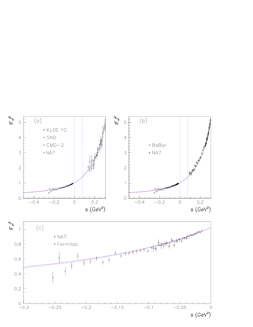
Figure 19: The Pion Form Factor around $s=0$. The $\pi^{+}\pi^{-}$ annihilation data submitted to the global fit are $only$ the NSK and KLOE10 samples. The full curve is the fit function derived when including also the spacelike data from NA7 [35] and Fermilab [36]; the dashed curve ris associated with the fit excluding the spacelike data. The BaBar data – shown in (b) for illustration – are not submitted to the fit. KLOE08 has no data point located within the plotted window. For clarity, only the data from NA7 [35] are shown in (a) and (b). In (c), one magnifies the spacelike region and plot the data [35, 36], used or not within the fit procedure. The vertical lines in (a) and (b) show the locations $s=0$ and $s=4m_{\pi}^{2}$.

On the other hand, it is worth noting the behavior of the predicted pion form factor in the region $m_{\pi\pi}<0.5$ GeV down to the negative $s$ region. Figure 19 shows that the pion form factor derived from fits describes quite well the (highly constraining) spacelike data down to about $-0.15$ GeV². Whether spacelike data are included within the data sample submitted to fit (full curve) or not (dashed curve) does not make any difference (both curves coincide within the thickness of the lines). This is a noticeable property as, following Section 6 in [19] and reminded in the Appendix, the NA7 data should be rescaled. The rescaling factor $1-\lambda$ is such that $\lambda$ depends on the spacelike data, on their scale uncertainties (0.8 % for NA7 [35]) and on the fitting function. Therefore, by ascertaining the threshold behavior of the pion form factor, Figure 19 proves that the contribution of the $\pi\pi$ threshold region to $g-2$ predicted using the NSK and KLOE10 data is reliable and confirmed by the existing spacelike data. Indeed, these are well accounted for without any regard to their being included within the data sample submitted to fit (see Figure (19c)).

6.4.3 The HLS Favored Estimate for $a_{\mu}^{th}$

From the discussion above, it follows that the preferred solution is those derived using NSK+KLOE10+$\tau$. Its estimate for $\Delta a_{\mu}$ carries a statistical significance of $4.88\sigma$. On the other hand, Figure 18 has shown that using or not the $\tau$ spectra does not significantly modify the significance for $\Delta a_{\mu}$ ($5.0\sigma\to 4.9\sigma$). In contrast, Figure 18 also shows that using the KLOE10 data sample increases the significance by about $0.5\sigma$.

In view of all these considerations, especially the issues encountered with the $\phi$ region physics information, the most motivated estimate we can propose is :

$$\left\{\begin{array}[]{lr}a_{\mu}^{th}=(11~{}659~{}169.55+\left[{}^{+1.26}_{-0.59}\right]_{\phi}+\left[{}^{+0.00}_{-2.00}\right]_{\tau}\pm 5.21_{th})~{}10^{-10}~{}~{},&\\[14.22636pt] \Delta a_{\mu}=a_{\mu}^{exp}-a_{\mu}^{th}=(39.35+\left[{}^{+0.59}_{-1.26}\right]_{\phi}+\left[{}^{+2.00}_{-0.00}\right]_{\tau}\pm 5.21_{th}\pm 6.3_{exp})~{}10^{-10}~{}~{},&\\[14.22636pt] a_{\mu}^{LO-HVP}=(681.82+\left[{}^{+1.26}_{-0.59}\right]_{\phi}+\left[{}^{+0.00}_{-2.00}\right]_{\tau}\pm 4.51_{th})~{}10^{-10}~{}~{}.\end{array}\right.$$ (19)

The quoted $[\delta a_{\mu}^{th}]_{\phi}$ is an estimate of the possible uncertainties affecting the $\phi$ region and emphasized in Subsection 5.2.1 and also just above; the central value is derived from a fit within configuration B and avoiding the use the SND phase constraint. $[\delta a_{\mu}^{th}]_{\phi}$ should not be added in quadrature to the theoretical error but linearly to the central value. Accounting for this possible shift slightly lessens the significance for $\Delta a_{\mu}$ from $4.81\sigma\to 4.67\sigma$. The uncertainty attributed to $\tau$ effects, is also as a possible shift and plays in the opposite direction.

Therefore, Figure 18 illustrates that the global fit approach allows for a gain in the significance for $\Delta a_{\mu}$ of about $1\sigma$ or more compared to the traditional methods based on numerical integration of the experimental cross sections [8, 6, 7, 9]. Moreover, our approach has allowed us to define the largest set of data samples which exhibit full consistency with each other.

The results involving the fit of the scan $\oplus$ (all/selected) ISR data, do not lead to a noticeably smaller uncertainty for $\Delta a_{\mu}$ compared to using only scan data, as already inferred in [13]. Indeed, Figure 18 indicates that in changing the fit conditions [scan $\oplus\tau]\to$ [scan $\oplus\tau\oplus$ KLOE10], the uncertainty marginally improves ($5.28\to 5.21$), while the central value moves by 3 units ($36.88\to 39.91$), increasing the significance ($4.5\sigma\to 4.9\sigma$).

7 Conclusion and Perspectives

The $e^{+}e^{-}\to\pi^{+}\pi^{-}$ annihilation channel has been widely studied and one is faced with several data sets collected by different groups under various conditions. Beside the scan experiments performed by the CMD-2 and SND collaborations which have produced valuable data samples [26, 27, 28, 29], experiments using the Initial State Radiation (ISR) method have also been performed by the KLOE and BaBar collaborations and have produced (much) higher statistics data samples [31, 32, 33]. The noticeable gain in statistics – for what concerns the $\pi^{+}\pi^{-}$ intermediate state – is partly balanced by the issues raised by the dominance of systematic uncertainties. Indeed, comparing the properties of these data samples reveals inconsistencies which leads to somewhat contradictory conclusions concerning the predicted value for the muon anomalous moment.

It thus becomes a relevant challenge to find a tool able to examine critically the properties of the various available samples and substantiate their differences. The present study proves that the existing data for :

• The $e^{+}e^{-}$ annihilation to the $\pi^{0}\gamma$, $\eta\gamma$, $\pi^{+}\pi^{-}\pi^{0}$, $K^{+}K^{-}$, $K^{0}\overline{K}^{0}$ final states,

• The dipion spectra in the $\tau^{\pm}\rightarrow\pi^{\pm}\pi^{0}\nu$ decay,

• Some radiative decays (namely, $\pi^{0}/\eta/\eta^{\prime}\to\gamma\gamma$, $\rho^{\pm}\to\pi^{\pm}\gamma$, $K^{*}\to K\gamma$, $\eta^{\prime}\to\omega\gamma$, $\phi\to\eta^{\prime}\gamma$) as given in the RPP,

supplemented with some limited isospin breaking (IB) information, provide a benchmark able to reconstruct with a noticeable precision the pion form factor measured in the $e^{+}e^{-}\to\pi^{+}\pi^{-}$ annihilation. As could have been expected, the requested IB pieces should cover the $\omega/\phi\to\pi^{+}\pi^{-}$ decays, but also the $\rho^{0}\to e^{+}e^{-}$ decay, rarely stressed explicitly [7].

The tool for this prediction is the broken HLS model (BHLS) defined and studied in [13]. In this last reference, the scan data for the $e^{+}e^{-}\to\pi^{+}\pi^{-}$ annihilation channel were used. However, the present study shows that replacing these data by only the $\rho^{0}/\omega/\phi$ decay data just referred to, allows BHLS to pin down all the parameters of the model and provide strikingly precise predictions for $e^{+}e^{-}\to\pi^{+}\pi^{-}$. These have been named ”$\tau$+PDG” predictions of the pion form factor. As these predictions are clearly a new way to formulate $\tau$ based predictions for the HVP, BHLS provides also a new tool to explore the long reported $\tau$ versus $e^{+}e^{-}$ discrepancy between the HVP evaluations.

Then, the present study leads to the following conclusions :

• 1/ There is no mismatch between $\tau$ based predictions and direct $e^{+}e^{-}$ evaluation of the HVP if one relies on BHLS and, especially, on its isospin breaking scheme. This is essentially implemented in two steps : direct breaking at the HLS Lagrangian level followed by vector meson mixing. The vector meson mixing, which generates physical vector fields, is unavoidable because, at first order in breaking parameters, the ideal vector fields are no longer mass eigenstates. This simply confirms the study in [13].

• 2/ The $\tau$+PDG predictions compare astonishingly to the KLOE data samples all along the spectra. Because of their influence on the PDG information, it is somewhat paradoxical to observe a difference between the NSK data and the $\tau$+PDG predictions, more marked than with both KLOE data samples. However, a $1\sigma$ modification of the width for $\omega\to\pi^{+}\pi^{-}$ allows to recover a good agreement between the NSK data and the $\tau$+PDG predictions. In contrast, the predicted pion form factor reveals an important disagreement with BaBar data, essentially concentrated in the $[0.74,0.78]$ GeV region.

• 3/ By varying the fit conditions, it has been found that the KLOE10 and the scan (NSK) data samples together lead to global fits with outstanding statistical properties. Even if the KLOE08 data sample has properties similar to KLOE10 (see Figures 10 and 9), it looks premature to include it within the global fit procedure.

From our analysis, one also gets  :

$$F_{\omega}\equiv{\rm Br}(\omega\to e^{+}e^{-})\times{\rm Br}(\omega\to\pi^{+}\pi^{-})=(1.166\pm 0.036)~{}10^{-6}~{},$$

close to the presently accepted [24] value and twice more precise, with a corresponding Orsay phase of $104.73^{\circ}\pm 0.63^{\circ}$. This value is in accord with the values derived from separate fits to scan, KLOE10 and KLOE08 data samples, reflecting that the lineshape of their pion form factors are consistent with each other. In contrast, the $F_{\omega}$ value derived from (global) fit to the BaBar data sample is different by about $(7\div 8)\sigma$.

Concerning the $\phi$ meson region, our analysis of BaBar data provides ${\rm Br}(\phi\to e^{+}e^{-})\times{\rm Br}(\phi\to\pi^{+}\pi^{-})=(3.31\pm 0.99)~{}10^{-8}$ in good agreement with the accepted value [24]. The corresponding Orsay phase, however, seems to disagree with expectations [72]; our fits tend to favor $-48.23^{\circ}\pm 1.88^{\circ}$, much closer to the SND phase.

Using the KLOE10 and the scan data samples leads to the most probable value for the muon anomalous moment :

$$a_{\mu}^{th}=(11~{}659~{}169.55+\left[{}^{+1.26}_{-0.59}\right]_{\phi}+\left[{}^{+0.00}_{-2.00}\right]_{\tau}\pm 5.21_{th})~{}10^{-10}~{},~{}$$

which exhibits a significance for $\Delta a_{\mu}=a_{\mu}^{exp}-a_{\mu}^{th}$ at a $(4.7\div 4.9)\sigma$ level, significantly larger than the results fully derived by direct numerical integration of the experimental cross sections. This estimate is free of any reweighting going beyond the reported uncertainties affecting the data samples involved in the derivation.

Some additional remarks are worth being made concerning this result and our approach :

• 4/ The cross sections which should be integrated within the BHLS model to evaluate $a_{\mu}^{th}$ can be considered as an ”effective field theory induced interpolation” between data points. By using a relatively fine energy binning, the interpolation uncertainties are certainly minimized in all regions, and for all cross sections, which exhibit sharp energy variations. This is certainly an advantage over the standard method which should rely on trapezoidal estimation between relatively distant measured data points, possibly improved by taking somewhat into account the local curvatures.

• 5/ One has certainly noted that the value for $a_{\mu}^{th}$ we privilege is smaller than all estimates involving $all$ ISR data. As explained above, this is because the effects of the KLOE sample is not balanced by the BaBar data. However, as noted several times above, the value for $F_{\omega}$ is a criterion which leads us to conclude that NSK and KLOE10 only have homogeneous properties which justifies to privilege a global simultaneous fit of these.

• 6/ The description of the BaBar data within the global fit framework does not look worse than in the really standalone fit published by this Collaboration. Actually, the main issue is not that much the description of the BaBar data sample stricto sensu than its consistency with the underlying physics correlations with other channels implied by the global approach within the same energy range. As, it is unlikely that BHLS may have some inherent reason to exhibit some tropism towards the scan or KLOE data, we indeed consider the $a_{\mu}^{th}$ value we propose as the most motivated one on statistical grounds. Of course, new ISR data one can expect from Belle are clearly valuable.

Nevertheless, the results derived using all $\pi^{+}\pi^{-}$ ISR data samples have been examined (see Figure 17) and shown to agree with the favored estimate just quoted. Because of the properties expected from the (BHLS) global framework recalled in the Introduction, using only the KLOE10 and NSK data samples provides already as precise results as those derived using all available ISR data samples and the traditional evaluation method of $a_{\mu}^{LO-HVP}$. This allows to avoid arguing on the relevance of (re)weighting procedures, which are always delicate matters.

Our work tells that the significance for $\Delta a_{\mu}$ starts to be close to the $5\sigma$ level. How close to this value it could be, should be confirmed by more precise annihilation data in the $[0.95~{},1.05]$ GeV mass region, especially in the $\pi^{+}\pi^{-}$, $\pi^{+}\pi^{-}\pi^{0}$ final states. Finally, new measurements for the experimental value of the muon $g-2$ are planned [85, 86]; they are important so as to confirm the central value for $a_{\mu}^{exp}$, and also to lessen the experimental uncertainty which starts now to be dominant when estimating the significance for $\Delta a_{\mu}$.

Appendices

Appendix A Graphical Account of Correlated Uncertainties

Most of the $\pi\pi$ data we are dealing with are subject to systematic bin–to–bin correlated uncertainties. In the most simple case, this is only a constant (not $s$–dependent) scale uncertainty with a supposed standard deviation $\sigma$. In this case, the $\chi^{2}$ to be minimized can be written :

$$\chi^{2}=\displaystyle\left[m-M-A\lambda\right]^{T}V^{-1}\left[m-M-A\lambda\right]+\frac{\lambda^{2}}{\sigma^{2}}$$ (20)

where $m$ is the vector of measurements, $M$ is the corresponding vector of model values and $V$ is the statistical error covariance matrix, which generally absorbs the parts of systematics which are not bin–to–bin correlated. An appropriate choice is $A=m$. $\lambda$ is the parameter which reflects the scale uncertainty; it can be considered as a random variable and each particular experiment can be viewed as a particular sampling of this. Assuming $\lambda$ independent of the measurements and of the model parameters, its particular value is fixed by solving $\partial\chi^{2}/\partial\lambda=0$ which yields :

$$\lambda=\frac{A^{T}V^{-1}\left[m-M\right]}{A^{T}V^{-1}A+\displaystyle\frac{1}{\sigma^{2}}}$$ (21)

Substituting this into Eq. (20) leads to the standard $\chi^{2}$ to be minimized when dealing with a constant bin–to–bin correlated uncertainty (global scale error) :

$$\begin{array}[]{ll}\chi^{2}=\displaystyle\left[m-M\right]^{T}W^{-1}(\sigma^{2})\left[m-M\right]~{}~{}~{},{}{}&\displaystyle\left(W(\sigma^{2})=[V+\sigma^{2}AA^{T}]\right)\end{array}$$ (22)

When plotting superimposed the data and the model function, or their difference (standard residual distribution), the drawing may be in $visual$ contradiction with the final $\chi^{2}$ obtained when minimizing Eq. (21). This generally happens when the scale uncertainty is not very small. However, Eq. (20) clearly tells that it is not $m$ which should compared to $M$ but $m-\lambda A$; this has been accounted for while plotting the spacelike data [35, 36] in Figure (19). A similar issue is encountered with the (standard) residuals $m_{i}-M_{i}$ and is solved by plotting the ”corrected residuals” $m_{i}-M_{i}-\lambda A_{i}$ rather than $m_{i}-M_{i}$.

With the advent of ISR data, the structure of systematic uncertainties has become much more complicated : there is generally a large number of independent bin–to–bin correlated uncertainties (10 for BaBar [33], 5 for KLOE08 [31], 13 for KLOE10 [32] …). In all cases [33, 31, 32] most of these are additionally $s$–dependent.

So, let us assume for definiteness that some data sample – represented by its measurement vector $m$ of length $n_{i}$ and its $n_{i}\times n_{i}$ statistical error covariance matrix $V$ – is subject to $n_{\alpha}$ independent bin–to–bin and $s$–dependent correlated uncertainties. These are generally considered as independent random variables of zero means and are supposed to carry $s$–dependent standard deviations ($\sigma_{\alpha}(s)$, $\alpha=1,\cdots n_{\alpha}$). In this case, Eq. (20) should be generalized to :

$$\chi^{2}=\displaystyle\left[m-M-B_{\alpha}\lambda_{\alpha}\right]^{T}V^{-1}\left[m-M-B_{\beta}\lambda_{\beta}\right]+\lambda_{\alpha}\lambda_{\beta}\delta_{\alpha\beta}$$ (23)

(summation over repeated greek indices is understood), defining the $n_{\alpha}$ vectors $B_{\alpha}$ by their components $[B_{\alpha}]_{i}=\sigma_{\alpha}(s_{i})m_{i}$ and using otherwise obvious notations.

In this case, the $\lambda_{\alpha}$ parameters can be considered as independent random variables each of zero mean and of unit standard deviation. Eq. (23) shows that $n_{\alpha}$ scale parameters are to be fixed, one for each of the bin–to–bin correlated uncertainty functions. A trivial mathematical recurrence, using in sequence the solution for $\partial\chi^{2}/\partial\lambda_{\alpha}=0$ (cf. Eq. (21)), allows to prove that the $\chi^{2}$ to be minimized becomes :

$$\begin{array}[]{ll}\chi^{2}=\displaystyle\left[m-M\right]^{T}W^{-1}\left[m-M\right]~{}~{}~{},{}{}&\displaystyle\left(W=[V+\sum_{\alpha}B_{\alpha}B_{\alpha}^{T}]\right).\end{array}$$ (24)

Then, one simply gets $W_{ij}=[V_{ij}+\sum_{\alpha}\sigma_{\alpha}(s_{i})\sigma_{\alpha}(s_{j})m_{i}m_{j}]$ as expected for independent bin–to–bin correlated uncertainties. No explicit knowledge of the values for the various $\lambda_{\alpha}$ is needed for this derivation.

For graphical purpose however, one may be interested in getting numerically the various $\lambda_{\alpha}$ values. One can easily prove that they are solutions of the linear system :

$$\begin{array}[]{lll}\displaystyle\sum_{\beta}\left[\delta_{\alpha\beta}+G_{\alpha\beta}\right]\lambda_{\beta}=H_{\alpha}~{}~{}~{}{\rm with{}}&G_{\alpha\beta}=B_{\alpha}^{T}V^{-1}B_{\beta}~{}~{}~{}{\rm and{}}&H_{\alpha}=B_{\alpha}^{T}V^{-1}\left[m-M\right]\end{array}$$ (25)

which is certainly always regular for systematics small compared with the data.

In this case, plotting together $m-\sum_{\alpha}\lambda_{\alpha}B_{\alpha}$ and $M$ gives a more appropriate representation than plotting $m$ and $M$; on the other hand, $m-\sum_{\alpha}\lambda_{\alpha}B_{\alpha}-M$ better reflects the $\chi^{2}$ value derived by minimizing Eq. (24) than $m-M$.

This does not exhaust all issues due to bin–to–bin correlations in the graphical representation of data and fits; indeed, at least the spread of the model function (when derived from fits) adds a usefull piece of information. Anyway, as all other correlations (especially those due the statistical errors) are not considered, plotting $m-\sum_{\alpha}\lambda_{\alpha}B_{\alpha}$ cannot exhaust the full issue but it certainly goes closer to facts.

References

- [1] T. Aoyama, M. Hayakawa, T. Kinoshita, and M. Nio, (2012), 1205.5368, Tenth-Order QED Contribution to the Electron g-2 and an Improved Value of the Fine Structure Constant.
- [2] T. Aoyama, M. Hayakawa, T. Kinoshita, and M. Nio, (2012), 1205.5370, Complete Tenth-Order QED Contribution to the Muon g-2.
- [3] M. Passera, Phys.Rev. D75, 013002 (2007), hep-ph/0606174, Precise mass-dependent QED contributions to leptonic g-2 at order and .
- [4] F. Jegerlehner and A. Nyffeler, Phys. Rept. 477, 1 (2009), 0902.3360, The Muon g-2.
- [5] J. Prades, E. de Rafael, and A. Vainshtein, (2009), 0901.0306, Hadronic Light-by-Light Scattering Contribution to the Muon Anomalous Magnetic Moment.
- [6] M. Davier, A. Hoecker, B. Malaescu, and Z. Zhang, Eur. Phys. J. C71, 1515 (2011), 1010.4180, Reevaluation of the Hadronic Contributions to the Muon g-2 and to alpha(MZ).
- [7] F. Jegerlehner and R. Szafron, (2011), 1101.2872, mixing in the neutral channel pion form factor and its role in comparing with spectral functions.
- [8] M. Davier et al., Eur. Phys. J. C66, 127 (2010), 0906.5443, The Discrepancy Between and Spectral Functions Revisited and the Consequences for the Muon Magnetic Anomaly.
- [9] T. Teubner, K. Hagiwara, R. Liao, A. D. Martin, and D. Nomura, (2010), 1001.5401, Update of g-2 of the muon and Delta alpha.
- [10] G. Ecker, J. Gasser, A. Pich, and E. de Rafael, Nucl.Phys. B321, 311 (1989), The Role of Resonances in Chiral Perturbation Theory.
- [11] J. Prades, Z. Phys. C63, 491 (1994), hep-ph/9302246, Massive spin 1 field chiral Lagrangian from an extended Nambu-Jona-Lasinio model of QCD.
- [12] G. Ecker, J. Gasser, H. Leutwyler, A. Pich, and E. de Rafael, Phys.Lett. B223, 425 (1989), Chiral Lagrangians for Massive Spin 1 Fields.
- [13] M. Benayoun, P. David, L. DelBuono, and F. Jegerlehner, Eur.Phys.J. C72, 1848 (2012), 1106.1315, Upgraded Breaking Of The HLS Model: A Full Solution to the and Decay Issues And Its Consequences On g-2 VMD Estimates.
- [14] M. Bando, T. Kugo, and K. Yamawaki, Phys. Rept. 164, 217 (1988), Nonlinear Realization and Hidden Local Symmetries.
- [15] M. Harada and K. Yamawaki, Phys. Rept. 381, 1 (2003), hep-ph/0302103, Hidden local symmetry at loop: A new perspective of composite gauge boson and chiral phase transition.
- [16] M. Bando, T. Kugo, and K. Yamawaki, Nucl. Phys. B259, 493 (1985), On the Vector Mesons as Dynamical Gauge Bosons of Hidden Local Symmetries.
- [17] M. Benayoun and H. B. O’Connell, Phys. Rev. D58, 074006 (1998), hep-ph/9804391, SU(3) breaking and hidden local symmetry.
- [18] M. Benayoun, P. David, L. DelBuono, O. Leitner, and H. B. O’Connell, Eur. Phys. J. C55, 199 (2008), hep-ph/0711.4482, The Dipion Mass Spectrum In Annihilation and tau Decay: A Dynamical (, , ) Mixing Approach.
- [19] M. Benayoun, P. David, L. DelBuono, and O. Leitner, Eur. Phys. J. C65, 211 (2010), 0907.4047, A Global Treatment Of VMD Physics Up To The : I. Annihilations, Anomalies And Vector Meson Partial Widths.
- [20] M. Benayoun, P. David, L. DelBuono, and O. Leitner, Eur. Phys. J. C68, 355 (2010), 0907.5603, A Global Treatment Of VMD Physics Up To The phi: II. Decay and Hadronic Contributions To g-2.
- [21] ALEPH, S. Schael et al., Phys. Rept. 421, 191 (2005), hep-ex/0506072, Branching ratios and spectral functions of tau decays: Final ALEPH measurements and physics implications.
- [22] CLEO, S. Anderson et al., Phys. Rev. D61, 112002 (2000), hep-ex/9910046, Hadronic structure in the decay .
- [23] Belle, M. Fujikawa et al., Phys. Rev. D78, 072006 (2008), 0805.3773, High-Statistics Study of the Decay.
- [24] Particle Data Group, K. Nakamura et al., J. Phys. G37, 075021 (2010), Review of Particle Physics.
- [25] L. M. Barkov et al., Nucl. Phys. B256, 365 (1985), Electromagnetic Pion Form-Factor in the Timelike Region.
- [26] CMD-2, R. R. Akhmetshin et al., Phys. Lett. B578, 285 (2004), hep-ex/0308008, Reanalysis of hadronic cross section measurements at CMD- 2.
- [27] CMD-2, R. R. Akhmetshin et al., Phys. Lett. B648, 28 (2007), hep-ex/0610021, High-statistics measurement of the pion form factor in the rho-meson energy range with the CMD-2 detector.
- [28] R. R. Akhmetshin et al., JETP Lett. 84, 413 (2006), hep-ex/0610016, Measurement of the cross section with the CMD-2 detector in the 370-MeV - 520-MeV cm energy range.
- [29] M. N. Achasov et al., J. Exp. Theor. Phys. 103, 380 (2006), hep-ex/0605013, Update of the cross section measured by SND detector in the energy region 400-MeV 1000-MeV.
- [30] M. Davier, A. Hoecker, B. Malaescu, C. Z. Yuan, and Z. Zhang, (2009), 0908.4300, Reevaluation of the hadronic contribution to the muon magnetic anomaly using new cross section data from BABAR.
- [31] KLOE, G. Venanzoni et al., (2009), 0906.4331, A precise new KLOE measurement of with ISR events and determination of contribution to for GeV.
- [32] KLOE, F. Ambrosino et al., (2010), 1006.5313, Measurement of ) from threshold to 0.85 using Initial State Radiation with the KLOE detector.
- [33] BABAR, B. Aubert et al., Phys. Rev. Lett. 103, 231801 (2009), 0908.3589, Precise measurement of the cross section with the Initial State Radiation method at BABAR.
- [34] BABAR Collaboration, J. Lees et al., Phys.Rev. D86, 032013 (2012), 1205.2228, Precise Measurement of the Cross Section with the Initial-State Radiation Method at BABAR.
- [35] NA7, S. R. Amendolia et al., Nucl. Phys. B277, 168 (1986), A Measurement of the Space - Like Pion Electromagnetic Form-Factor.
- [36] E. B. Dally et al., Phys. Rev. Lett. 48, 375 (1982), Elastic Scattering Measurement of the Negative Pion Radius.
- [37] ATLAS, G. Aad et al., Phys. Lett. B716, 1 (2012), 1207.7214, Observation of a new particle in the search for the Standard Model Higgs boson with the ATLAS detector at the LHC.
- [38] CMS, S. Chatrchyan et al., Phys. Lett. B716, 30 (2012), 1207.7235, Observation of a new boson at a mass of 125 GeV with the CMS experiment at the LHC.
- [39] Muon G-2, G. W. Bennett et al., Phys. Rev. D73, 072003 (2006), hep-ex/0602035, Final report of the muon E821 anomalous magnetic moment measurement at BNL.
- [40] B. L. Roberts, Chin. Phys. C34, 741 (2010), 1001.2898, Status of the Fermilab Muon Experiment.
- [41] J. Gasser and H. Leutwyler, Annals Phys. 158, 142 (1984), Chiral Perturbation Theory to One Loop.
- [42] J. Gasser and H. Leutwyler, Nucl. Phys. B250, 465 (1985), Chiral Perturbation Theory: Expansions in the Mass of the Strange Quark.
- [43] D. Ebert and H. Reinhardt, Phys.Lett. B173, 453 (1986), EFFECTIVE CHIRAL MESON LAGRANGIAN WITH WEINBERG AND KSRF RELATIONS FROM MICROSCOPIC FOUR QUARK INTERACTIONS.
- [44] A. Dhar, R. Shankar, and S. R. Wadia, Phys.Rev. D31, 3256 (1985), Nambu-Jona-Lasinio Type Effective Lagrangian. 2. Anomalies and Nonlinear Lagrangian of Low-Energy, Large N QCD.
- [45] J. Prades, Z.Phys. C63, 491 (1994), hep-ph/9302246.
- [46] J. Prades, Eur. Phys. J. C11, 571 (1999), hep-ph/9302246.
- [47] G. ’t Hooft, Nucl. Phys. B72, 461 (1974), A Planar Diagram Theory For Strong Interactions.
- [48] A. Manohar, (2001), Hadrons in the 1/N expansion.
- [49] H. Leutwyler, Nucl. Phys. Proc. Suppl. 64, 223 (1998), hep-ph/9709408, On the 1/N-expansion in chiral perturbation theory.
- [50] R. Kaiser and H. Leutwyler, (0600), hep-ph/9806336, Pseudoscalar decay constants at large .
- [51] A. Bramon, A. Grau, and G. Pancheri, Phys. Lett. B345, 263 (1995), hep-ph/9411269, Effective chiral lagrangians with an SU(3) broken vector meson sector.
- [52] A. Bramon, A. Grau, and G. Pancheri, Phys. Lett. B344, 240 (1995), Radiative vector meson decays in SU(3) broken effective chiral Lagrangians.
- [53] M. Hashimoto, Phys. Rev. D54, 5611 (1996), hep-ph/9605422, Hidden local symmetry for anomalous processes with isospin/SU(3) breaking effects.
- [54] G. ’t Hooft, Phys. Rept. 142, 357 (1986), How Instantons Solve the U(1) Problem.
- [55] T. Fujiwara, T. Kugo, H. Terao, S. Uehara, and K. Yamawaki, Prog. Theor. Phys. 73, 926 (1985), Nonabelian Anomaly and Vector Mesons as Dynamical Gauge Bosons of Hidden Local Symmetries.
- [56] V. Cirigliano, G. Ecker, and H. Neufeld, Phys. Lett. B513, 361 (2001), hep-ph/0104267, Isospin violation and the magnetic moment of the muon.
- [57] J. Bijnens and P. Gosdzinsky, Phys. Lett. B388, 203 (1996), hep-ph/9607462, Electromagnetic contributions to vector meson masses and mixings.
- [58] V. Cirigliano, G. Ecker, and H. Neufeld, JHEP 08, 002 (2002), hep-ph/0207310, Radiative tau decay and the magnetic moment of the muon.
- [59] F. Flores-Baez, A. Flores-Tlalpa, G. Lopez Castro, and G. Toledo Sanchez, Phys. Rev. D74, 071301 (2006), hep-ph/0608084, Long-distance radiative corrections to the di-pion tau lepton decay.
- [60] A. Flores-Tlalpa, F. Flores-Baez, G. Lopez Castro, and G. Toledo Sanchez, Nucl. Phys. Proc. Suppl. 169, 250 (2007), hep-ph/0611226, Model-dependent radiative corrections to revisited.
- [61] F. Flores-Baez, G. L. Castro, and G. Toledo Sanchez, Phys.Rev. D76, 096010 (2007), 0708.3256, The Width difference of rho vector mesons.
- [62] W. J. Marciano and A. Sirlin, Phys. Rev. Lett. 71, 3629 (1993), Radiative corrections to pi(lepton 2) decays.
- [63] E. Braaten and C.-S. Li, Phys.Rev. D42, 3888 (1990), Electroweak radiative corrections to the semihadronic decay rate of the tau lepton.
- [64] E. Braaten, S. Narison, and A. Pich, Nucl.Phys. B373, 581 (1992), QCD analysis of the tau hadronic width.
- [65] J. Erler, Rev.Mex.Fis. 50, 200 (2004), hep-ph/0211345, Electroweak radiative corrections to semileptonic tau decays.
- [66] G. J. Gounaris and J. J. Sakurai, Phys. Rev. Lett. 21, 244 (1968), Finite width corrections to the vector meson dominance prediction for .
- [67] CMD-2 Collaboration, R. Akhmetshin et al., (1999), hep-ex/9904027, Measurement of cross-section with CMD-2 around rho meson.
- [68] OPAL, K. Ackerstaff et al., Eur. Phys. J. C7, 571 (1999), hep-ex/9808019, Measurement of the strong coupling constant and the vector and axial-vector spectral functions in hadronic tau decays.
- [69] S. Ghozzi and F. Jegerlehner, Phys.Lett. B583, 222 (2004), hep-ph/0310181, Isospin violating effects in e+ e- versus tau measurements of the pion form-factor —F(pi)—**2(s).
- [70] M. Benayoun et al., Eur. Phys. J. C2, 269 (1998), hep-ph/9707509, New results in meson physics.
- [71] C. E. Wolfe and K. Maltman, Phys. Rev. D80, 114024 (2009), 0908.2391, Models of Isospin Breaking in the Pion Form Factor: Consequences for the Determination of and .
- [72] M. N. Achasov et al., Phys. Lett. B474, 188 (2000), hep-ex/0001048, Decay .
- [73] M. Benayoun, www2.fz-juelich.de/ikp//mesonnet/2012_ff_workshop/venue.shtml , Confronting the scan, ISR and tau dipion spectra within a global model.
- [74] S. Eidelman, private communication .
- [75] H. Leutwyler, Phys.Lett. B374, 181 (1996), hep-ph/9601236, Implications of mixing for the decay .
- [76] C. A. Dominguez, (2011), 1103.5864, Quark masses in QCD: a progress report.
- [77] G. Colangelo et al., (2010), 1011.4408, Review of lattice results concerning low energy particle physics.
- [78] M. Benayoun, L. DelBuono, and H. B. O’Connell, Eur. Phys. J. C17, 593 (2000), hep-ph/9905350, VMD, the WZW Lagrangian and ChPT: The third mixing angle.
- [79] Y.-H. Chen, Z.-H. Guo, and H.-Q. Zheng, Phys.Rev. D85, 054018 (2012), 1201.2135, Study of mixing from radiative decay processes.
- [80] KLOE, F. Ambrosino et al., Phys. Lett. B648, 267 (2007), hep-ex/0612029, Measurement of the pseudoscalar mixing angle and eta’ gluonium content with KLOE detector.
- [81] A. Bernicha, G. Lopez Castro, and J. Pestieau, Phys.Rev. D50, 4454 (1994), Mass and width of the rho0 from an S matrix approach to .
- [82] A. Bernicha, G. Lopez Castro, and J. Pestieau, Phys.Rev. D53, 4089 (1996), hep-ph/9510435.
- [83] P. J. Mohr, B. N. Taylor, and D. B. Newell, (2012), 1203.5425, CODATA Recommended Values of the Fundamental Physical Constants: 2010.
- [84] KLOE Collaboration, D. Babusci et al., Phys.Lett. B720, 336 (2013), 1212.4524, Precision measurement of and determination of the contribution to the muon anomaly with the KLOE detector.
- [85] Fermilab P989 Collaboration, B. Lee Roberts, Nucl.Phys.Proc.Suppl. 218, 237 (2011), The Fermilab muon (g-2) project.
- [86] J-PARC New g-2/EDM experiment Collaboration, H. Iinuma, J.Phys.Conf.Ser. 295, 012032 (2011), New approach to the muon g-2 and EDM experiment at J-PARC.