Conservative Constraints on Early Cosmology: an illustration of the Monte Python cosmological parameter inference code

Abstract

Models for the latest stages of the cosmological evolution rely on a less solid theoretical and observational ground than the description of earlier stages like BBN and recombination. As suggested in a previous work by Vonlanthen et al., it is possible to tweak the analysis of CMB data in such way to avoid making assumptions on the late evolution, and obtain robust constraints on “early cosmology parameters”. We extend this method in order to marginalise the results over CMB lensing contamination, and present updated results based on recent CMB data. Our constraints on the minimal early cosmology model are weaker than in a standard $\Lambda$CDM analysis, but do not conflict with this model. Besides, we obtain conservative bounds on the effective neutrino number and neutrino mass, showing no hints for extra relativistic degrees of freedom, and proving in a robust way that neutrinos experienced their non-relativistic transition after the time of photon decoupling. This analysis is also an occasion to describe the main features of the new parameter inference code Monte Python, that we release together with this paper. Monte Python is a user-friendly alternative to other public codes like CosmoMC, interfaced with the Boltzmann code class.

1 Introduction

Models for the evolution of the early universe between a redshift of a few millions and a few hundreds have shown to be very predictive and successful: the self-consistency of Big Bang Nucleosynthesis (BBN) model could be tested by comparing the abundance of light elements and the result of Cosmic Microwave Background (CMB) observations concerning the composition of the early universe; the shape of CMB acoustic peaks matches accurately the prediction of cosmological perturbation theory in a Friedmann-Lemaître Universe described by general relativity, with a thermal history described by standard recombination. The late cosmological evolution is more problematic. Models for the acceleration of the universe, based on a cosmological constant, or a dark energy component, or departures from general relativity, or finally departure from the Friedmann-Lemaître model at late times, have shown no predictive power so far. The late thermal history, featuring reionization from stars, is difficult to test with precision. Overall, it is fair to say that “late cosmology” relies on less solid theoretical or observational ground than “early cosmology”.

When fitting the spectrum of temperature and polarisation CMB anisotropies, we make simultaneously some assumptions on early and late cosmology, and obtain intricate constraints on the two stages. However, Vonlanthen et al. [1] suggested a way to carry the analysis leading to constraints only on the early cosmology part. This is certainly interesting since such an analysis leads to more robust and model-indepent bounds than a traditional analysis affected by priors on the stages which are most poorly understood. The approach of [1] avoids making assumptions on most relevant “late cosmology-related effects”: projection effects due to the background evolution, photon rescattering during reionization, and the late Integrated Sachs Wolfe (ISW) effect.

In this work, we carry a similar analysis, pushed to a higher precision level since we also avoid making assumptions on the contamination of primary CMB anisotropies by weak lensing. We use the most recent available data from the Wilkinson Microwave Anisotropy Probe (WMAP) and South Pole Telescope (SPT) data, and consider the case of a minimal “early cosmology” model, as well as extended models with free density of ultra-relativistic relics or massive neutrinos.

This analysis is an occasion to present a new cosmological parameter inference code. This Monte Carlo code written in Python, called Monte Python, offers a convenient alternative to CosmoMC [4]. It is interfaced with the Boltzmann code class [2, 3]. Monte Python is released publicly together with this work.

In section 2, we explain the method allowing to get constraints only on the early cosmological evolution. We present our result for the minimal early cosmology model in section 3, and for two extended models in section 4. In section 5, we briefly summarize some of the advantages of Monte Pyhton, without entering into technical details (presented anyway in the code documentation). Our conclusions are highlighted in section 6.

2 How to test early cosmology only?

The spectrum of primary CMB temperature anisotropies is sensitive to various physical effects:

• (C1) the location of the acoustic peaks in multipole space depends on the sound horizon at decoupling $d_{s}(\tau_{rec})$ (an “early cosmology”-dependent parameter) divided by the angular diameter distance to decoupling $d_{A}(\tau_{rec})$ (a “late cosmology”-dependent parameter, sensitive to the recent background evolution: acceleration, spatial curvature, etc.)

• (C2) the contrast between odd and even peaks depends on $\omega_{b}/\omega_{\gamma}$, i.e. on “early cosmology”.

• (C3) the amplitude of all peaks further depends on the amount of expansion between radiation-to-matter equality and decoupling, governing the amount of perturbation damping at the beginning of matter domination, and on the amount of early integrated Sachs-Wolfe effect enhancing the first peak just after decoupling. These are again “early cosmology” effects (in the minimal $\Lambda$CDM model, they are both regulated by the redshift of radiation-to-matter equality, i.e by $\omega_{m}/\omega_{r}$).

• (C4) the enveloppe of high-$\ell$ peaks depends on the diffusion damping scale at decoupling $\lambda_{d}(\tau_{rec})$ (an “early cosmology” parameter) divided again by the angular diameter distance to decoupling $d_{A}(\tau_{rec})$ (a “late cosmology” parameter).

• (C5-C6) the global shape depends on initial conditions through the primordial spectrum amplitude $A_{s}$ (C5) and tilt $n_{s}$ (C6), which are both “early cosmology” parameters.

• (C7) the slope of the temperature spectrum at low $\ell$ is affected by the late integrated Sachs Wolfe effect, i.e. by “late cosmology”. This effect could actually be considered as a contamination of the primary spectrum by secondary anisotropies, which are not being discussed in this list.

• (C8) the global amplitude of the spectrum at $\ell\gg 40$ is reduced by the late reionization of the universe, another “late cosmology” effect. The amplitude of this suppression is given by $e^{-2\tau}$, where $\tau$ is the reionization optical depth.

In summary, primary CMB temperature anisotropies are affected by late cosmology only through: (i) projection effects from real space to harmonic space, controlled by $d_{A}(\tau_{rec})$; (ii) the late ISW effect, affecting only small $\ell$’s; and (iii) reionization, suppressing equally all multipoles at $\ell\gg 40$ . These are actually the sectors of the cosmological model which are most poorly constrained and understood. But we see that the shape of the power spectrum at $\ell\gg 40$, interpreted modulo an arbitrary scaling in amplitude ($C_{\ell}\rightarrow\alpha C_{\ell}$) and in position ($C_{\ell}\rightarrow C_{\beta\ell}$), contains information on early cosmology only. This statement is very general and valid for extended cosmological models. In the case of the $\Lambda$CDM models, it is illustrated by figure 1, in which we took two different $\Lambda$CDM models (with different late-time geometry and reionization history), and rescaled one of them with a shift in amplitude given by $e^{-2\tau-\tau^{\prime}}$ and in scale given by $d_{A}/d_{A}^{\prime}$. At $\ell\gg 40$, the two spectra are identical. For more complicated cosmological models sharing the same physical evolution until approximately $z\sim 100$, a similar rescaling and matching would work equally well.

Figure 1: Dimensionless temperature (left) and E-polarization (right) unlensed spectra of two $\Lambda$CDM models with the same value of “early cosmology” parameters ($\omega_{b}$, $\omega_{cdm}$, $A_{s}$, $n_{s}$) (fixed to WMAP best-fitting values), and different values of “late cosmology” parameters: ($\Omega_{\Lambda}$, $z_{reio}$) = (0.720,10) (solid curves) or (0.619, 5) (dashed curve). The dashed curves have been rescaled vertically by the ratio of $e^{-2\tau}$ and horizontally by the ratio of $d_{A}(\tau_{rec})$ in each model, using the values of $\tau$ and $d_{A}(\tau_{rec})$ calculated by class for each model. At $\ell=40$, the difference between the dashed and solid line in the temperature plot is under $2\,\mu$K². At $\ell=80$, it is already below $1\,\mu$K².

If polarization is taken into account, the same statement remains valid. The late time evolution affects the polarization spectrum through the angular diameter distance to decoupling $d_{A}(\tau_{rec})$ and through the impact of reionization, which also suppresses the global amplitude at $\ell\gg 40$, and generates an additional feature at low $\ell$’s, due to photon re-scatering by the inhomogeneous and ionized inter-galactic medium. The shape of the primary temperature and polarization spectrum at $\ell\gg 40$, interpreted modulo a global scaling in amplitude and in position, only contains information on the early cosmology.

However, the CMB spectrum that we observe today gets a contribution from secondary anisotropies and foregrounds. In particular, the observed CMB spectra are significantly affected by CMB lensing caused by large scale structures. This effect depends on the small scale matter power spectrum, and therefore on late cosmology (acceleration, curvature, neutrinos becoming non-relativistic at late time, possible dark energy perturbations, possible departures from Einstein gravity on very large scales, etc.). In the work of [1], this effect was mentioned but not dealt with, because of the limited precision of WMAP5 and ACBAR data compared to the amplitude of lensing effects, at least within the multipole range studied in that paper ($40\leq\ell\leq 800$). The results that we will present later confirm that this simplification was sufficient and did not introduce a significant “late cosmology bias”. However, with the full WMAP7+SPT data (that we wish to use up to the high multipoles), it is not possible to ignore lensing, and in order to probe only early cosmology, we are forced to marginalize over the lensing contamination, in the sense of the method described below. By doing so, we will effectively get rid of the major two sources of secondary (CMB) anisotropies, the late ISW effect and CMB lensing. We neglect the impact of other secondary effects like the Rees-Sciama effect. As far as foregrounds are concerned, the approach of WMAP and SPT consists in eliminating them with a spectral analysis, apart from residual foregrounds which can be fitted to the data, using some nuisance parameters which are marginalized over. By following this approach, we also avoid to introduce a “late cosmology bias” at the level of foregrounds.

Let us now discuss how one can marginalize over lensing corrections. Ideally, we should lens the primary CMB spectrum with all possible lensing patterns, and marginalize over the parameters describing these patterns. But the lensing of the CMB depends on the lensing potential spectrum $C_{\ell}^{\phi\phi}$, that can be inferred from the matter power spectrum at small redshift, $P(k,z)$. We should marginalize over all possible shapes for $C_{\ell}^{\phi\phi}$, i.e. over an infinity of degrees of freedom. We need to find a simpler approach.

One can start by noticing that modifications of the late-time background evolution caused by a cosmological constant, a spatial curvature, or even some inhomogeneous cosmology models, tend to affect matter density fluctuations in a democratic way: all Fourier modes being inside the Hubble radius and on linear scales are multiplied by the same redshift-dependent growth factor. CMB lensing is precisely caused by such modes. Hence, for this category of models, differences in the late-time background evolution lead to a different amplitude for $C_{\ell}^{\phi\phi}$, and also a small tilt since different $\ell$’s probe the matter power spectrum at different redshifts. Hence, if we fit the temperature and polarization spectrum at $\ell\gg 40$ modulo a global scaling in amplitude, a global shift in position, and additionally an arbitrary scaling and tilting of the lensing spectrum $C_{\ell}^{\phi\phi}$ that one would infer assuming $\Lambda$CDM, we still avoid making assumption about the late-time evolution.

There are also models introducing a scale-dependent growth factor, i.e. distortions in the shape of the matter power spectrum. This is the case in presence of massive neutrinos or another hot dark matter component, of dark energy with unusually large perturbations contributing to the total perturbed energy-momentum tensor, or in modified gravity models. In principle, these effects could lead to arbitrary distortions of $C_{\ell}^{\phi\phi}$ as a function of $\ell$. Fortunately, CMB lensing only depends on the matter power spectrum $P(k,z)$ integrated over a small range of redshifts and wave numbers. Hence it makes sense to stick to an expansion scheme: at first order we can account for the effects of a scale-dependent growth factor by writing the power spectrum as the one predicted by $\Lambda$CDM cosmology, multiplied by arbitrary rescaling and tilting factors; and at the next order, one should introduce a running of the tilt, then a running of the running, etc. By marginalizing over the rescaling factor, tilting factor, running, etc., one can still fit the CMB spectra without making explicit assumptions about the late-time cosmology. In the result section, we will check that the information on early cosmology parameters varies very little when we omit to marginalize over the lensing amplitude, or when we include this effect, or when we also marginalize over a tilting factor. Hence we will not push the analysis to the level of an arbitrary lensing running factor.

3 Results assuming a minimal early cosmology model

We assume a “minimal early cosmology” model described by four parameters ($\omega_{b}$, $\omega_{cdm}$, $A_{s}$, $n_{s}$). In order to extract constraints independent of the late cosmological evolution, we need to fit the CMB temperature/polarisation spectrum measured by WMAP (seven year data [5]) and SPT [6] only above a given value of $\ell$ (typically $\ell\sim 40$), and to marginalize over two factors accounting for vertical and a horizontal scaling. In practice, there are several ways in which this could be implemented.

For the amplitude, we could fix the reionization history and simply marginalize over the amplitude parameter $A_{s}$. By fitting the data at $\ell\gg 40$, we actually constrain the product $e^{-2\tau_{reio}}A_{s}$, i.e. the primordial amplitude rescaled by the reionization optical depth $\tau_{reio}$, independently of the details of reionization. In our runs, we fix $\tau_{reio}$ to an arbitrary value, and we vary $A_{s}$; but in the Markov chains, we keep memory of the value of the derived parameter $e^{-2\tau_{reio}}A_{s}$. By quoting bounds on $e^{-2\tau}A_{s}$ rather than $A_{s}$, we avoid making explicit assumptions concerning the reionization history.

For the horizontal scaling, we could modify class in such way to use directly $d_{A}(\tau_{rec})$ as an input parameter. For input values of ($\omega_{b}$, $\omega_{cdm}$, $d_{A}(\tau_{rec})$), class could in principle find the correct spectrum at $\ell\gg 40$. It is however much simpler to use the unmodified code and pass values of the five parameters ($\omega_{b}$, $\omega_{cdm}$, $A_{s}$, $n_{s}$, $h$). In our case, $h$ should not be interpreted as the reduced Hubble rate, but simply as a parameter controlling the value of the physical quantity $d_{A}(\tau_{rec})$. For any given set of parameters, the code computes the value that $d_{A}(\tau_{rec})$ would take in a $\Lambda$CDM model with the same early cosmology and with a Hubble rate $H_{0}=100h$km/s/Mpc. It then fits the theoretical spectrum to the data. The resulting likelihood should be associated to the inferred value of $d_{A}(\tau_{rec})$ rather than to $h$. The only difference between this simplified approach and that in which $d_{A}(\tau_{rec})$ would be passed as an input parameter is that in one case, one assumes a flat prior on $d_{A}(\tau_{rec})$, and in the other case a flat prior on $h$. But given that the data allows $d_{A}(\tau_{rec})$ to vary only within a very small range where it is almost a linear function of $h$, the prior difference has a negligible impact.

To summarize, in order to get constraints on “minimal early cosmology”, it is sufficient to run Markov Chains in the same way as for a minimal $\Lambda$CDM model with parameters ($\omega_{b}$, $\omega_{cdm}$, $A_{s}$, $n_{s}$, $\tau$, $h$), excepted that:

• we do not fit the lowest temperature/polarization multipoles to the data;

• we fix $\tau$ to an arbitrary value;

• we do not plot nor interpret the posterior probability of the parameters $A_{s}$ and $h$. We only pay attention to the posterior probability of the two derived parameters $e^{-2\tau}A_{s}$ and $d_{A}(\tau_{rec})$, which play the role of the vertical and horizontal scaling factors, and which are marginalized over when quoting bounds on the remaining three “early cosmology parameters” ($\omega_{b}$, $\omega_{cdm}$, $n_{s}$).

Hence, for a parameter inference code, this is just a trivial matter of defining and storing two “derived parameters”. For clarity, we will refer to the runs performed in this way as the “agnostic” runs.

	$100~{}\omega_{b}$	$\omega_{cdm}$	$n_{s}$	${d_{A}}^{rec}$	$10^{9}e^{-2\tau}A_{s}$	$A_{lp}$	$n_{lp}$
	$\Lambda$CDM
	$2.241_{-0.044}^{+0.043}$	$0.1114_{-0.0048}^{+0.0048}$	$0.960_{-0.011}^{+0.011}$	$12.93_{-0.12}^{+0.11}$	$2.069_{-0.092}^{+0.085}$
	same lensing potential as in $\Lambda$CDM
$\ell\geq 40$	$2.204_{-0.047}^{+0.048}$	$0.1160_{-0.0059}^{+0.0056}$	$0.946_{-0.014}^{+0.014}$	$12.85_{-0.13}^{+0.13}$	$2.20_{-0.13}^{+0.12}$
$\ell\geq 60$	$2.203_{-0.053}^{+0.050}$	$0.1163_{-0.0065}^{+0.0063}$	$0.945_{-0.016}^{+0.016}$	$12.84_{-0.14}^{+0.14}$	$2.20_{-0.15}^{+0.13}$
$\ell\geq 80$	$2.190_{-0.057}^{+0.053}$	$0.1180_{-0.0073}^{+0.0067}$	$0.940_{-0.018}^{+0.019}$	$12.81_{-0.15}^{+0.15}$	$2.26_{-0.18}^{+0.15}$
$\ell\geq 100$	$2.184_{-0.056}^{+0.054}$	$0.1187_{-0.0079}^{+0.0067}$	$0.935_{-0.019}^{+0.020}$	$12.80_{-0.15}^{+0.16}$	$2.29_{-0.20}^{+0.16}$
	marginalization over lensing potential amplitude
$\ell\geq 100$	$2.159_{-0.064}^{+0.060}$	$0.1227_{-0.0088}^{+0.0083}$	$0.926_{-0.022}^{+0.022}$	$12.73_{-0.17}^{+0.18}$	$2.39_{-0.23}^{+0.20}$	$0.88_{-0.13}^{+0.12}$
	marginalization over lensing potential amplitude and tilt
$\ell\geq 100$	$2.160_{-0.068}^{+0.064}$	$0.1222_{-0.0094}^{+0.0088}$	$0.927_{-0.024}^{+0.024}$	$12.74_{-0.18}^{+0.18}$	$2.38_{-0.25}^{+0.20}$	$0.78_{-0.15}^{+0.20}$	$-0.16_{-0.33}^{+0.55}$

Table 1: Limits at the $68\%$ confidence level of the mininum credible interval of model parameters. The $\Lambda$CDM model of the first line has a sixth independent parameter ($z_{reio}$) that we do not show. We do not show either the limits on the three nuisance parameters associated to the SPT likelihood.

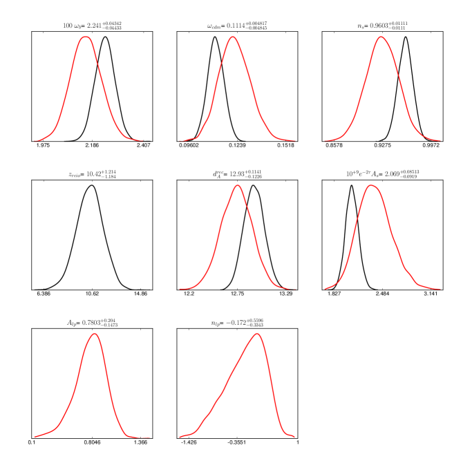
Figure 2: Constraints on the five parameters of the minimal early cosmology model (red), compared to usual constraints on the minimal $\Lambda$CDM model (black). The $\Lambda$CDM has a sixth independent parameter, the reionization optical depth. The constraints on early cosmology (called “agnostic constraints” in the text) includes a marginalization over the amplitude and tilt of the matter power spectrum leading to CMB lensing. We do not show here the posterior of the three nuisance parameter used to fit SPT data.

In the second line of Table 1, we show the bounds obtained with such an agnostic run, for a cut-off value $\ell=40$. These results can be compared with those of a minimal $\Lambda$CDM model, obtained through the same machinery but with all multipoles $\ell\geq 2$. Since the agnostic bounds rely on less theoretical assumptions, they are slightly wider. Interestingly, the central value of $\omega_{b}$ and $n_{s}$ are smaller in absence of late-cosmology priors, and larger for $\omega_{cdm}$. Still the $\Lambda$CDM results are compatible with the agnostic results, which means that on the basis of this test, we cannot say that $\Lambda$CDM is a bad model. Our agnostic bounds on ($\omega_{b}$, $\omega_{cdm}$, $n_{s}$) are simply more model-independent and robust, and one could argue that when using CMB bounds in the study of BBN, in CDM relic density calculations or for inflationary model building, one should better use those bounds in order to avoid relying on the most uncertain assumptions of the minimal cosmological model, namely $\Lambda$ domination and standard reionization.

The decision to cut the likelihood at $\ell\geq 40$ was somewhat arbitrary. Figure 1 shows that two rescaled temperature spectra with different late-time cosmology tend only gradually towards each other above $\ell\sim 40$. We should remove enough low multipoles in order to be sure that late time cosmology has a negligible impact given the data error bars. We tested this dependence by cutting the likelihood at $\ell\geq 60$, $\ell\geq 80$ or $\ell\geq 100$. When increasing the cut-off from 40 to 100, we observe variations in the mean value that are less important than from 2 to 40. To have the more robust constraints, we will then take systematically the cut-off of $\ell=100$, which is the one more likely to avoid any contamination from “late time cosmology”.

Until now, our analysis is not completely “agnostic”, because we did not marginalize over lensing. We fitted the data with a lensed power spectrum, relying on the same lensing potential as an equivalent $\Lambda$CDM model with the same values of ($\omega_{b}$, $\omega_{cdm}$, $n_{s}$, $e^{-2\tau}A_{s}$, $d_{A}(\tau_{rec})$). To deal with lensing, we introduce three new parameters ($A_{lp}$, $n_{lp}$, $k_{lp}$) in class. Given the traditional input parameters ($\omega_{b}$, $\omega_{cdm}$, $A_{s}$, $n_{s}$, $h$), the code first computes the Newtonian potential $\phi(k,z)$. This potential is then rescaled as

$$\phi(k,z)\longrightarrow A_{lp}\left(\frac{k}{k_{lp}}\right)^{n_{lp}}\phi(k,z)~{}.$$ (3.1)

Hence, the choice ($A_{lp}$, $n_{lp}$)=(1,0) corresponds to the standard lensing potential predicted in the $\Lambda$CDM model. Different values correspond to an arbitrary rescaling or tilting of the lensing potential, which can be propagated consistently to the lensed CMB temperature/polarization spectrum.

The sixth run shown in Table 1 corresponds to $n_{lp}=0$ and a free parameter $A_{lp}$. The minimum credible interval for this rescaling parameter is $A_{lp}=0.88^{+0.12}_{-0.13}$ at the 68% Confidence Level (CL), and is compatible with one. This shows that WMAP7+SPT data alone are sensitive to lensing, and well compatible with the lensing signal predicted by the minimal $\Lambda$CDM model. It is also interesting to note that the bounds on other cosmological parameter move a little bit, but only by a small amount (compared to the difference between the $\Lambda$CDM and the previous “agnostic” runs), showing that “agnostic bounds” are robust.

In the seventh line of Table 1, we also marginalize over the tilting parameter $n_{lp}$ (with unbounded flat prior). A priori, this introduces a lot of freedom in the model. Nicely, this parameter is still well constrained by the data ($n_{lp}=-0.16^{+0.55}_{-0.33}$ at 68%CL), and compatible with the $\Lambda$CDM prediction $n_{lp}=0$. Bounds on other parameters vary this time by a completely negligible amount: this motivates us to stop the expansion at the level of $n_{lp}$, and not to test the impact of running. The credible interval for $A_{lp}$ is the only one varying significantly when $n_{lp}$ is left free, but this result depends on the pivot scale $k_{lp}$, that we choose to be equal to $k_{lp}=0.1$/Mpc, so that the amplitude of the lensing spectrum $C_{\ell}^{\phi\phi}$ is nearly fixed at $\ell\sim 100$. By tuning the pivot scale, we could have obtained bounds on $A_{s}$ nearly equal for the case with/without free $n_{lp}$. The posterior probability of each parameter marginalized over other parameters is shown in Figure 2, and compared with the results of the standard $\Lambda$CDM analysis.

Our results nicely agree with those of [1]. These authors found a more pronounced drift of the parameters ($\omega_{b}$, $\omega_{cdm}$, $n_{s}$) with the cut-off multipole than in the first part of our analysis, but this is because we use data on a wider multipole range and have a larger lever arm. Indeed, Ref.  [1] limited their analysis of WMAP5 plus ACBAR data to $\ell\leq 800$, arguing that above this value, lensing would start playing an important role. In our analysis, we include WMAP7 plus 47 SPT band powers probing up to $\ell\sim 3000$, but for consistency we must simultaneously marginalize over lensing. Indeed, the results of Ref.  [1] are closer to our results with lensing marginalization (the fully “agnostic” ones) that without. Keeping only one digit in the error bar, we find ($100\omega_{b}=2.16\pm 0.07$, $\omega_{cdm}=0.122\pm 0.009$, $n_{s}=0.93\pm 0.02$), when this reference found ($100\omega_{b}=2.13\pm 0.05$, $\omega_{cdm}=0.124\pm 0.007$, $n_{s}=0.93\pm 0.02$). The two sets of results are very close to each other, but our central values for $\omega_{b}$ and $\omega_{cdm}$ are slightly closer to the $\Lambda$CDM one. The fact that we get slightly larger error bars in spite of using better data in a wider multipole range is related to our lensing marginalization: we see that by fixing lensing, this previous analysis was implicitly affected by a partial “late cosmology prior”, but only at a very small level.

Our results from the last run can be seen as robust “agnostic” bounds on ($\omega_{b}$, $\omega_{cdm}$, $n_{s}$), only based on the “minimal early cosmology” assumption. They are approximately twice less constraining than ordinary $\Lambda$CDM models, and should be used in conservative studies of the physics of BBN, CDM decoupling and inflation.

4 Effective neutrino number and neutrino mass

We can try to generalize our analysis to extended cosmological models. It would make no sense to look at models with spatial curvature, varying dark energy or late departures from Einstein gravity, since all these assumptions would alter only the late time evolution, and our method is designed precisely in such way that the results would remain identical. However, we can explore models with less trivial assumptions concerning the early cosmological evolution. This includes for instance models with:

• a free primordial helium fraction $Y_{He}$. So far, we assumed $Y_{He}$ to be a function of $\omega_{b}$, as predicted by standard BBN (this is implemented in class following the lines of Ref. [7]). Promoting $Y_{He}$ as a free parameter would be equivalent to relax the assumption of standard BBN. Given the relatively small sensitivity of current CMB data to $Y_{He}$ [5], we do not perform such an analysis here, but this could be done in the future using e.g. Planck data.

• a free density of relativistic species, parametrized by a free effective neutrino number $N_{\rm eff}$, differing from its value of $3.046$ in the minimal $\Lambda$CDM model [8]. This parameter affects the time of equality between matter and radiation, but this effect can be cancelled at least at the level of “early cosmology” by tuning appropriately the density of barons and CDM. Even in that case, relativistic species will leave a signature on the CMB spectrum, first through a change in the diffusion damping scale $\lambda_{d}(\tau_{rec})$, and second through direct effects at the level of perturbations, since they induce a gravitational damping and phase shifting of the photon fluctuation [9, 10]. It is not obvious to anticipate up to which level these effects are degenerate with those of other parameters. Hence it is interesting to run Markov chains and search for “agnostic bounds” on $N_{\rm eff}$.

• neutrino masses (or for simplicity, three degenerate masses $m_{\nu}$ summing up to $M_{\nu}=3m_{\nu}$). Here we are not interested in the fact that massive neutrinos affect the background evolution and change the ratio between the redshift of radiation-to-matter equality, and that of matter-to-$\Lambda$ equality. This is a “late cosmology” effect that we cannot probe with our method, since we are not sensitive to the second equality. However, for masses of the order of $m_{\nu}\sim 0.60$ eV, neutrinos become non-relativistic at the time of photon decoupling. Even below this value, the mass leaves a signature on the CMB spectrum coming from the fact that, first, they are not yet ultra-relativistic at decoupling, and second, the transition to the non-relativistic regime takes place when the CMB is still probing metric perturbations through the early integrated Sachs-Wolfe effect. Published bounds on $M_{\nu}$ from CMB data alone probe all these intricate effects [5], and it would be instructive to obtain robust bounds based only on the mass impact on “early cosmology”.

$100~{}\omega_{b}$	$\omega_{cdm}$	$n_{s}$	$N_{\rm eff}$	${d_{A}}^{rec}$	$10^{9}e^{-2\tau}A_{s}$	$A_{lp}$	$n_{lp}$
$\Lambda$CDM
$2.279_{-0.056}^{+0.053}$	$0.124_{-0.013}^{+0.011}$	$0.979_{-0.019}^{+0.019}$	$3.77_{-0.66}^{+0.58}$	$12.35_{-0.53}^{+0.46}$	$2.01_{-0.10}^{+0.10}$
$\ell\geq 100$, marginalization over lensing potential amplitude and tilt
$2.03_{-0.16}^{+0.13}$	$0.113_{-0.015}^{+0.011}$	$0.862_{-0.077}^{+0.065}$	$2.04_{-1.26}^{+0.78}$	$13.59_{-0.87}^{+0.96}$	$2.84_{-0.59}^{+0.49}$	$0.69_{-0.18}^{+0.21}$	$-0.23_{-0.43}^{+0.57}$

Table 2: Limits at the 68% confidence level of the minimum credible interval of model parameters. The $\Lambda$CDM+$N_{\rm eff}$ model of the first line has a seventh independent parameter ($z_{reio}$) that we do not show. We do not show either the limits on the three nuisance parameters associated to the SPT likelihood.

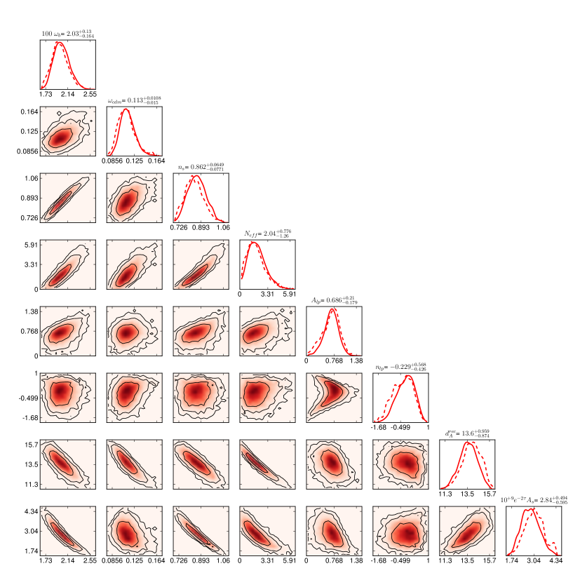
Figure 3: One and two-dimensional posterior distribution (solid line) of the parameters of the “agnostic” run with a free effective neutrino number. The dashed line stands for the average likelihood distribution. The concentric contour lines in the two-dimensional posteriors stand for 68, 95 and 99% CL.

For the effective neutrino number, we performed two runs similar to our previous $\Lambda$CDM and “fully agnostic” run (with marginalization over lensing amplitude and tilt), in presence of one additional free parameter $N_{\rm eff}$. Our results are summarized in Table 2 and Figure 3. In the $\Lambda$CDM+$N_{\rm eff}$ case, we get $N_{\rm eff}=3.77^{+0.58}_{-0.66}$ (68% CL), very close to the result of [11], $N_{\rm eff}=3.85\pm 0.62$ (differences in the priors can explain this insignificant difference). It is well-known by now that the combination of WMAP and small-scale CMB data shows a marginal preference for extra relativistic degrees of freedom in the seven-parameter model. The surprise comes from our “agnostic” bound on this number, $N_{\rm eff}=2.04^{+0.78}_{-1.26}$ (68% CL). As explained before, this bound cannot come from a change in the time of equality, nor in the scale of the first peak, nor in the late integrated Sachs-Wolfe effect; it can only result from the measurement of the the sound horizon $d_{s}(\tau_{rec})$ relatively to the diffusion damping scale $\lambda_{d}(\tau_{rec})$, and from the direct effects of extra relativistic degrees of freedom on photon perturbations. Hence it is normal that $N_{\rm eff}$ is much less constrained in the agnostic runs, but the interesting conclusion is that without assuming $\Lambda$CDM at late time, the CMB does not favor high values of $N_{\rm eff}$. It is compatible with the standard value $N_{\rm eff}=3.046$ roughly at the one-$\sigma$ level, with even a marginal preference for smaller values. This shows that recent hints for extra relativistic relics in the universe disappear completely if we discard any information on the late time cosmological evolution. It is well-known that $N_{\rm eff}$ is very correlated with $H_{0}$ and affected by the inclusion of late cosmology data sets, like direct measurement of $H_{0}$ or of the BAO scale. Our new result shows that even at the level of CMB data only, the marginal hint for large $N_{\rm eff}$ is driven by physical effects related to late cosmology (and in particular by the angular diameter distance to last scattering as predicted in $\Lambda$CDM).

The triangle plot in Figure 3 shows that in the agnostic run, $N_{\rm eff}$ is still very correlated with other parameters such as $\omega_{b}$, $\omega_{cdm}$ and $n_{s}$. Low values of $N_{\rm eff}$ (significantly smaller than the standard value 3.046) are only compatible with a very small $\omega_{b}$, $\omega_{cdm}$ and $n_{s}$. Note that in this work, we assume standard BBN in order to predict $Y_{He}$ as a function of $\omega_{b}$ (and of $N_{\rm eff}$ when this parameter is also left free), but we do not incorporate data on light element abundances. By doing so, we would favor the highest values of $\omega_{b}$ in the range allowed by the current analysis ($\omega_{b}\sim 0.022$), and because of parameter correlations we would also favor the highest values of $\omega_{cdm}$, $n_{s}$ and $N_{\rm eff}$, getting close to the best-fitting values in the minimal early cosmology model with $N_{\rm eff}\sim 3.046$.

$100~{}\omega_{b}$	$\omega_{cdm}$	$n_{s}$	$M_{\nu}$ (eV)	${d_{A}}^{rec}$	$10^{9}e^{-2\tau}A_{s}$	$A_{lp}$	$n_{lp}$
$\Lambda$CDM
$2.205_{-0.049}^{+0.046}$	$0.114_{-0.0050}^{+0.0052}$	$0.949_{-0.013}^{+0.014}$	$<1.4$	$12.86_{-0.13}^{+0.13}$	$2.16_{-0.12}^{+0.10}$
$\ell\geq 100$, marginalization over lensing potential amplitude and tilt
$2.136_{-0.072}^{+0.065}$	$0.123_{-0.010}^{+0.009}$	$0.920_{-0.025}^{+0.025}$	$<1.8$	$12.69_{-0.19}^{+0.19}$	$2.43_{-0.28}^{+0.21}$	$0.81_{-0.16}^{+0.22}$	$-0.11_{-0.32}^{+0.58}$

Table 3: Limits at the 68% confidence level of the minimum credible interval of model parameters (excepted for $M_{\nu}$, for which we show the 95% CL upper limit). The $\Lambda$CDM+$M_{\nu}$ model of the first line has a seventh independent parameter ($z_{reio}$) that we do not show. We do not show either the limits on the three nuisance parameters associated to the SPT likelihood.

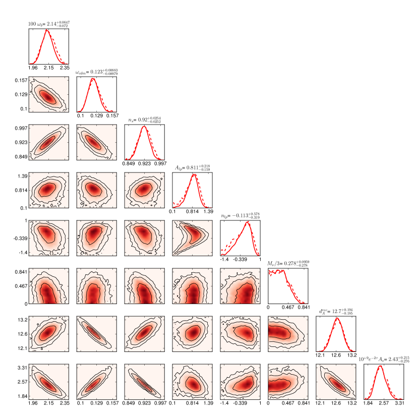
Figure 4: One and two-dimensional posterior distribution (solid line) of the parameters of the “agnostic” run with a total neutrino mass $M_{\nu}$ (assuming three degenerate neutrinos of individual mass $m_{\nu}$). Again, dashed line stands for average likelihood distribution, contour lines indicate the 68, 95 and 99% CL.

For neutrino masses, we performed two similar runs (summarised in Table 3 and Figure 4), with now $M_{\nu}$ being the additional parameter (assuming three degenerate neutrino species). In the $\Lambda$CDM case, our result $M_{\nu}<1.4$ eV (95%CL) is consistent with the rest of the literature, and close to the WMAP-only bound of [5]: measuring the CMB damping tail does not bring significant additional information on the neutrino mass. In the agnostic run, this constraint only degrades to $M_{\nu}<1.8$ eV (95%CL). This limit is consistent with the idea that for sufficiently large $m_{\nu}$, the CMB can set a limit on the neutrino mass not just through its impact on the background evolution at late time (and its contribution to $\omega_{m}$ today), but also through direct effects occurring at the time of recombination and soon after. It is remarkable that this is true even for neutrinos of individual mass $m_{\nu}\sim 0.6$ eV, becoming non-relativistic precisely at the time of photon decoupling. The conclusion that the CMB is not compatible with neutrinos becoming non-relativistic before $z_{rec}$ (and not even slightly before!) appears to be very robust, and independent of any constraint on the late cosmological evolution.

5 Advantages of Monte Python

The results of this paper were obtained with the new parameter inference code Monte Python, that we release publicly together with this article. Currently, Monte Python is interfaced with the Boltzmann code class, and explores parameter space with the Metropolis-Hastings algorithm, just like CosmoMC (note however that interfacing it with other codes and switching to other exploration algorithms would be easy, thanks to the modular architecture of the code). Hence, the difference with CosmoMC [4] does not reside in a radically different strategy, but in several details aiming at making the user’s life easy. It is not our goal to describe here all the features implemented in Monte Python: for that, we refer the reader to the documentation distributed with the code. We only present here a brief summary of the main specificities of Monte Python.

Language and compilation. As suggested by its name, Monte Python is a Monte Carlo code written in Python. This high-level language allows to code with a very concise style: Monte Python is compact, and the implementation of e.g. new likelihoods requires very few lines. Python is also ideal for wrapping other codes from different languages: Monte Python needs to call class, written in C, and the WMAP likelihood code, written in Fortran 90. The user not familiar with Python should not worry: for most purposes, Monte Python does not need to be edited, when CosmoMC would need to: this is explained in the fourth paragraph below.
Another advantage of Python is that it includes many libraries (and an easy way to add more), so that Monte Python is self-contained. Only the WMAP likelihood code needs its own external libraries, as usual. Python codes do not require a compilation step. Hence, provided that the user has Python 2.7 installed on his/her computer alongside very standard modules, the code only needs to be downloaded, and is ready to work with.

Modularity. A parameter inference code is based on distinct blocks: a likelihood exploration algorithm, an interface with a code computing theoretical predictions (in our case, a Boltzmann code solving the cosmological background and perturbation evolution), and an interface with each experimental likelihood. In Monte Python, all three blocks are clearly split in distinct modules. This would make it easy, e.g., to interface Monte Python with camb [12] instead of class, or to switch from the in-build Metropolis-Hastings algorithm to another method, e.g. a nested sampling algorithm.
The design choice of the code has been to write these modules as different classes, in the sense of C++, whenever it served a purpose. For instance, all likelihoods are defined as separated classes. It allows for easy and intuitive way of comparing two runs, and helps simplify the code. The cosmological module is also defined as a class, with a defined amount of functions. If someone writes a python wrapper for camb defining these same functions, then Monte Python would be ready to serve.
On the other hand the likelihood exploration part is contained in a normal file, defining only functions. The actual computation is only done in the file code/mcmc.py, so it is easy to implement a different exploration algorithm. From the rest of the code, this step would be as transparent as possible.
In Python, like in C++, a class can inherit properties from a parent class. This becomes particularly powerful when dealing with data likelihoods. Each likelihood will inherit from a basic likelihood class, able to read data files, and to treat storage. In order to implement a new likelihood, one then only needs to write the computation part, leaving the rest automatically done by the main code. This avoids several repetitions of the same piece of code. Furthermore, if the likelihood falls in a generic category, like CMB likelihoods based on reading a file in the format .newdat (same files as in CosmoMC), it will inherit more precise properties from the likelihood_newdat class, which is itself a daughter of the likelihood class. Hence, in order to incorporate CMB likelihoods apart from WMAP, one only needs to write one line of python for each new case: it is enough to tell, e.g., to the class accounting for the CMB experiment SPT that it inherits all properties from the generic likelihood_newdat class. Then, this class is ready to read a file in the .newdat format and to work. Note that our code already incorporates another generic likelihood class that will be useful in the future for reading Planck likelihoods, after the release of Planck data.
Finally, please note that these few lines of code to write for a new likelihood are completely outside the main code containing the exploration algorithm, and the cosmological module. You do not need to tell the rest of the code that you wrote something new, you just have to use your new likelihood by its name in a starting parameter file.

Memory keeping and safe running. Each given run, i.e. each given combination of a set of parameters to vary, a set of likelihoods to fit, and a version of the Boltzmann code, is associated to a given directory where the chains are written (e.g. it could be a directory called chains/wmap_spt/lcdm). All information about the run is logged automatically in this directory, in a file log.param, at the time when the first chain is started. This file contains the parameter names, ranges and priors, the list of extra parameters, the version of the Boltzmann code, the version and the characteristics of each data likelihood, etc. Hence the user will always remember the details of a previous run.
Moreover, when a new chain is started, the code reads this log file (taking full advantage of the class structure of the code). If the user started the new chain with an input file, the code will compare all the data in the input file with the data in the log.param file. If they are different, the code complains and stop. The user can then take two decisions: either some characteristic of the run has been changed without noticing, and the input file can be corrected. Or it has been changed on purpose, then this is a new run and the user must require a different output directory. This avoids the classical mistake of mixing unwillingly some chains that should not be compared to each other. Now, if the input file is similar to the log.param file, the chain will start (it will not take the same name as previous chains: it will append automatically to its name a number equal to the first available number in the chain directory). In addition, the user who wishes to launch new chains for the same run can omit to pass an input file: in this case all the information about the run is automatically read in the log.param and the chain can start.
The existence of log.param file has another advantage. When one wants to analyze chains and produce result files and plots (the equivalent of running Getdist and matlab or maple in the case of CosmoMC), one simply needs to tell Monte Python to analyze a given directory. It is not needed to pass another input file, since all information on parameter names and ranges will be found in the log.param. If the output needs to be customized (i.e., changing the name of the parameters, plotting only a few of them, rescaling them by some factor, etc.), then the user can use command lines and eventually pass one small input file with extra information.

No need to edit the code when adding parameters. The name of cosmological parameters is never defined in Monte Python. The code only knows that in the input file, it will read a list of parameter names (e.g. omega_b, z_reio, etc.) and pass this list to the cosmology code together with some values. The cosmology code (in our case, class) will read these names and values as if they were written in an input file. If one of the names is not understood by the cosmology code, the run stops. The advantage is that the user can immediately write in the input file any name understood by class, without needing to edit Monte Python. This is not the case with CosmoMC. This is why users can do lots of things with Monte Python without ever needing to edit it or even knowing Python. If one wants to explore a completely new cosmological model, it is enough to check that it is implemented in class (or to implement it oneself and recompile the class python wrapper). But Monte Python doesn’t need to know about the change. To be precise, in the Monte Python input file, the user is expected to pass the name, value, prior edge etc. of all parameters (i) to be varied; (ii) to be fixed; (iii) to be stored in the chains as derived parameters. These can be any class parameter: cosmological parameters, precision parameters, flags, input file names. Let us take two examples:

• In this paper, we showed some posterior probabilities for the angular diameter distance up to recombination. It turns out that this parameter is always computed and stored by class, under the name ‘da_rec’. Hence we only needed to write in the input file of Monte Python a line looking roughly like da_rec=‘derived’ (see the documentation for the exact syntax), and this parameter was stored in the chains. In this case Monte Python did not need editing.

• We used in this work the parameter $[e^{-2\tau}A_{s}]$. To implement this, there would be two possibilities. The public class version understands the parameters $\tau$ and $A_{s}$. The first possibility is to modify the class input module, teach it to check if there is an input parameter ‘exp_m_two_tau_A_s’, and if there is, to infer $A_{s}$ from $[e^{-2\tau}A_{s}]$ and $\tau$. Then there is no need to edit Monte Python. However, in a case like this, it is actually much simpler to leave class unchanged and to add two lines in the Monte Python file data.py. There is a place in this file devoted to internal parameter redefinition. The user can add two simple lines to tell Monte Python to map (‘exp_m_two_tau_A_s’, ‘tau’) to (‘A_s’, ‘tau’) before calling class. This is very basic and does not require to know python. All these parameter manipulations are particularly quick and easy with Monte Python.

The user is also free to rescale a parameter (e.g. $A_{s}$ to $10^{9}A_{s}$ in order to avoid dealing with exponents everywhere) by specifying a rescaling factor in the input file of Monte Python: so this can be done without editing neither Monte Python nor class.
Please note however that, while this is true that any input parameter will be understood directly by the code, to recover derived parameters, the wrapper routine (distributed with class) should know about them. To this end, we implemented what we think is a near-complete list of possible derived parameters in the latest version of the wrapper.

Playing with covariance matrices. When chains are analyzed, the covariance matrix is stored together with parameter names. When this matrix is passed as input at the beginning of the new run, these names are read. The code will then do automatically all the necessary matrix manipulation steps needed to get all possible information from this matrix if the list of parameter has changed: this includes parameter reordering and rescaling, getting rid of parameters in the matrix not used in the new runs, and adding to the matrix some diagonal elements corresponding to new parameters. All the steps are printed on screen for the user to make sure the proper matrix is used.

Friendly plotting. The chains produced by Monte Python are exactly in the same format as those produced by CosmoMC: the user is free to analyze them with GetDist or with a customized code. However Monte Python incorporates its own analysis module, that produce output files and one or two dimensional plots in PDF format (including the usual "triangle plot"). Thanks to the existence of log.param files, we just need to tell Monte Python to analyze a given directory - no other input is needed. Information on the parameter best-fit, mean, minimal credible intervals, convergence, etc., are then written in three output files with different presentation: a text file with horizontal ordering of the parameters, a text file with vertical ordering, and a latex file producing a latex table. In the plots, the code will convert parameter names to latex format automatically (at least in the simplest case) in order to write nice labels (e.g. it has a routine that will automatically replace tau_reio by \tau_$\{$reio$\}$). If the output needs to be customized (i.e., changing the name of the parameters, plotting only a few of them, rescaling them by some factor, etc.), then the user can use command lines and eventually pass one small input file with extra information. The code stores in the directory of the run only a few PDF files (by default, only two; more if the user asks for individual parameter plots), instead of lots of data files that would be needed if we were relying on an external plotting software like Matlab.

Convenient use of mock data. The released version of Monte Python includes simplified likelihood codes mimicking the sensitivity of Planck, of a Euclid-like galaxy redshift survey, and of a Euclid-like cosmic shear survey. The users can take inspiration from these modules to build other mock data likelihoods. They have been developed in such way that dealing with mock data is easy and fully automatized. The first time that a run is launched, Monte Python will find that the mock data file does not exist, and will create one using the fiducial model parameters passed in input. In the next runs, the power spectra of the fiducial model will be used as an ordinary data set. This approach is similar to the one developed in the code FuturCMB [13] compatible with CosmoMC, except that the same steps needed to be performed manually.

6 Conclusions

Models for the latest stages of the cosmological evolution rely on a less solid theoretical and observational ground than the description of earlier stages, like BBN and recombination. Reference [1] suggested a way to infer parameters from CMB data under some assumptions about early cosmology, but without priors on late cosmology. By standard assumption on early cosmology, we understand essentially the standard model of recombination in a flat Friedmann-Lemaître universe, assuming Einstein gravity, and using a consistency relation between the baryon and Helium abundance inferred from standard BBN. The priors on late cosmology that we wish to avoid are models for the acceleration of the universe at small redshift, a possible curvature dominated stage, possible deviations from Einstein gravity on very large scale showing up only at late times, and reionization models.

We explained how to carry such an analysis very simply, pushing the method of [1] to a higher precision level by introducing a marginalization over the amplitude and tilt of the CMB lensing potential. We analyzed the most recent available WMAP and SPT data in this fashion, that we called “agnostic” throughout the paper. Our agnostic bounds on the minimal “early cosmology” model are about twice weaker than in a standard $\Lambda$CDM analysis, but perfectly compatible with $\Lambda$CDM results: there is no evidence that the modeling of the late-time evolution of the background evolution, thermal history and perturbation growth in the $\Lambda$CDM is a bad model, otherwise it would tilt the constraints on $\omega_{b}$, $\omega_{cdm}$ and $n_{s}$ away from the “agnostic” results. It is interesting that WMAP and SPT alone favor a level of CMB lensing different from zero and compatible with $\Lambda$CDM predictions.

We extended the analysis to two non-minimal models changing the “early cosmology”, with either a free density of ultra-relativistic relics, or some massive neutrinos that could become non-relativistic before or around photon decoupling. In the case of free $N_{\rm eff}$, it is striking that the “agnostic” analysis removes any hint in favor of extra relics. The allowed range is compatible with the standard value $N_{\rm eff}=3.046$ roughly at the one-sigma level, with a mean smaller than three. In the case with free total neutrino mass $M_{\nu}$, it is remarkable that the “agnostic” analysis remains sensitive to this mass: the two-sigma bound coincides almost exactly with the value of individual masses corresponding to a non-relativistic transition taking place at the time of photon decoupling.

The derivation of these robust bounds was also for us an occasion to describe the main feature of the new parameter inference code Monte Python, that we release together with this paper. Monte Python is an alternative to CosmoMC, interfaced with the Boltzmann code class. It relies on the same basic algorithm as CosmoMC, but offers a variety of user-friendly function, that make it suitable for a wide range of cosmological parameter inference analyses.

References

- [1] M. Vonlanthen, S. Rasanen and R. Durrer, JCAP 1008 (2010) 023 [arXiv:1003.0810 [astro-ph.CO]].
- [2] J. Lesgourgues, arXiv:1104.2932 [astro-ph.IM].
- [3] D. Blas, J. Lesgourgues and T. Tram, JCAP 1107 (2011) 034 [arXiv:1104.2933 [astro-ph.CO]].
- [4] A. Lewis and S. Bridle, Phys. Rev. D 66 (2002) 103511 [astro-ph/0205436].
- [5] E. Komatsu et al. [WMAP Collaboration], Astrophys. J. Suppl. 192 (2011) 18 [arXiv:1001.4538 [astro-ph.CO]].
- [6] C. L. Reichardt, L. Shaw, O. Zahn, K. A. Aird, B. A. Benson, L. E. Bleem, J. E. Carlstrom and C. L. Chang et al., Astrophys. J. 755 (2012) 70 [arXiv:1111.0932 [astro-ph.CO]].
- [7] J. Hamann, J. Lesgourgues and G. Mangano, JCAP 0803 (2008) 004 [arXiv:0712.2826 [astro-ph]].
- [8] G. Mangano, G. Miele, S. Pastor and M. Peloso, Phys. Lett. B 534 (2002) 8 [astro-ph/0111408].
- [9] W. Hu and N. Sugiyama, Astrophys. J. 471 (1996) 542 [astro-ph/9510117].
- [10] S. Bashinsky and U. Seljak, Phys. Rev. D 69 (2004) 083002 [astro-ph/0310198].
- [11] R. Keisler, C. L. Reichardt, K. A. Aird, B. A. Benson, L. E. Bleem, J. E. Carlstrom, C. L. Chang and H. M. Cho et al., Astrophys. J. 743 (2011) 28 [arXiv:1105.3182 [astro-ph.CO]].
- [12] A. Lewis, A. Challinor and A. Lasenby, Astrophys. J. 538 (2000) 473 [astro-ph/9911177].
- [13] L. Perotto, J. Lesgourgues, S. Hannestad, H. Tu and Y. Y. Y. Wong, JCAP 0610 (2006) 013 [astro-ph/0606227].