A method to estimate the significance of coincident gravitational-wave observations from compact binary coalescence
Abstract
Coalescing compact binary systems consisting of neutron stars and/or black holes should be detectable with upcoming advanced gravitational-wave detectors such as LIGO, Virgo, GEO and KAGRA. Gravitational-wave experiments to date have been riddled with non-Gaussian, non-stationary noise that makes it challenging to ascertain the significance of an event. A popular method to estimate significance is to time shift the events collected between detectors in order to establish a false coincidence rate. Here we propose a method for estimating the false alarm probability of events using variables commonly available to search candidates that does not rely on explicitly time shifting the events while still capturing the non-Gaussianity of the data. We present a method for establishing a statistical detection of events in the case where several silver-plated (3–5) events exist but not necessarily any gold-plated () events. We use LIGO data and a simulated, realistic, blind signal population to test our method.
I Introduction
Detecting the gravitational-waves from coalescing neutron stars and or black holes should be possible with advanced GW detectors such as LIGO, Virgo, GEO and KAGRA rates2010 . If the performance of past detectors is any indicator of the performance of future GW detectors, they are likely to be affected by non-Gaussian noise slutsky2010 . Coincident observations are crucial in validating the detection of GWs but it is necessary to establish the probability that the coincident event could arise from noise alone.
If the detectors’ data were Gaussian and stationary, it would be straightforward to compute the false alarm probability (FAP) of a coincident event based solely on its signal-to-noise ratio (SNR) and the number of independent trials. With non-stationary, non-Gaussian data the SNR is not sufficient to describe the significance of an event and, furthermore, the distribution of detector noise is not known a priori.
Estimating false-coincident backgrounds from time delay coincidence associated with searches for GWs was first proposed for targeted compact binary coalescence GW searches in CBC:S1 . This method has been the commonest used in subsequent searches CBC:S2 ; LIGO:S2MACHO ; LIGO:S2BBH ; LIGO:TAMA ; LIGO:S3Spin ; CBC:S3S4 ; CBC:S51yr ; CBC:S5:12_18 ; CBC:S5LV ; CBCHM:S5 ; CBC:S6 . We present a method to estimate the false alarm probability of a GW event from coalescing compact objects without time shifts by measuring the false alarm probability distributions for non-coincident events using a set of common variables available to the searches. This greatly simplifies analysis and lends itself nicely to an online analysis environment.
This paper is organized as follows. In Sec. II we describe a formalism for ranking GW events and establishing the probability distribution for a given event’s rank in noise. In Sec. III we present how to estimate the significance of a population of CBC events, which might include silver-plated (i.e. less than ) events. In Sec. IV, we test our method with a mock, advanced detector search that uses four days of LIGO fifth science run (S5) data that has been recolored to have an Advanced LIGO spectrum containing a plausible, simulated, blind population of double neutron star binary mergers. We demonstrate that we can detect GWs from neutron star binaries with very low false alarm probability.
II Method
GW searches for compact binary coalescence begin by matched filtering data in the detectors findchirppaper . If peaks in SNR times series for more than one detector are consistent with the light travel time between detectors and timing errors, these peaks are considered to be a coincident event.
GW data to date have not been stationary and Gaussian slutsky2010 thus making it difficult to model the noise in GW searches. Non-stationary noise degrades the effectiveness of standard matched filter searches. For that reason additional signal consistency tests are often employed, such as explicit tests Allen:2004 ; HannaThesis . Non-stationarity occurs on several timescales. Here we are more concerned with short duration non-stationary bursts of noise called glitches for which tests are very useful discriminators.
In this section we will present a method using common variables available to a compact binary search to estimate the FAP without relying on time shifting the detector data. Although many variables and measurements may be used, in this paper we consider two parameters: the matched filter SNR and the statistic , which depend on the detector , as well as parameters intrinsic to the source that the template describes such as mass and spin, . In this section, we introduce the framework for evaluating the FAP of GW candidates.
II.1 Ranking events
Here is our concise definition of a coincident gravitational wave search for compact binary sources. i) The search consists of detectors. ii) We seek to find the significance of an event found in the D detectors localized in time. iii) The intrinsic parameters of the event will be unknown a priori. Our detection pipeline will measure the significance as a function of the parameters of the template waveform
For each detector of a detector network we use and to rank candidates with parameters from least likely to be a gravitational wave to most likely. We use a standard likelihood ratio Gregory:2005 defined as
| (1) |
where is the probability of observing given a signal, and is the probability of observing given noise. It is assumed that the signal distribution has been marginalized over all relevant parameters and the refers only to the template waveform parameters that are measured by the pipeline. We make the simplifying assumption Cannon2008 that the likelihood can be factored into products of likelihoods from individual detectors,
| (2) |
The simplification that the likelihood function can be built from these products implies statistical independence between detectors for both signals and noise. This results in a suboptimal ranking statistic. However, we can compute the FAP associated with this statistic, and in fact, it becomes much easier to do so.
II.2 Computing the FAP
The FAP is the probability of measuring a given if the data contains only noise. N.B., this is not the same as assessing the probability that the data contains only noise, which requires knowing the prior probabilities of both signal and noise. In constructing the FAP, , we start with
| (3) |
where is the surface of constant . From (2), we have, assuming that the likelihood values in noise are independent between the detectors,
| (4) |
where is obtained by marginalizing over , and in the single-detector terms,
| (5) |
where is the contour of constant in the {, } surface at constant . Implicit in (4) and (5) is the assumption that the coincidence criteria do not depend on , or . Finally, is obtained by marginalizing over ,
| (6) |
The probability of observing an event with a likelihood value at least as large as some threshold is
| (7) |
A GW search will typically produce multiple coincident events during a given experiment. That means that there will be multiple opportunities to produce an event with a certain likelihood value. We are ultimately interested in the probability of getting one or more events with after all the events are considered. The probability of getting at least one such event after forming independent coincidences111In practice it can be difficult to know if the coincidences formed are independent, however as long as they are related to the true number of independent trials by an overall scaling, one can adjust the number so that it agrees with the observed rate of coincidences for low significance events. This works because GWs are very rare and true signals will vastly underwhelm the false positives that a pipeline produces at high FAP. Thus the bias in calibrating to high FAP events is very small. can be adjusted by the complement of the binomial distribution
| (8) |
This is the FAP at in an experiment that yielded coincident events. In what follows, we will drop the explicit notation and simply use where it is assumed that we have corrected for the number of trials.
III GW Events as a Poisson Distribution
Historically, GW experiments have used rates to rank events CBC:S51yr ; CBC:S5:12_18 ; CBC:S5LV ; CBCHM:S5 ; CBC:S6 . Assuming that the likelihood function is independent of time over the duration of the experiment (or can be approximated as such) we can cluster the most significant events of the search over a duration longer than the correlation induced by the filter and we might expect the events arising from noise to obey Poisson statistics. In what follows we assume that in fact this is the case and connect our estimation of FAP with the false alarm rate (FAR) often quoted in gravitational wave searches for compact binary coalescence.
For a Poisson process with mean , the probability of observing or more events is given by the survival function
| (9) |
Using from (8), setting , and solving for tells us the mean number of noise events with ,
| (10) |
The quantity, inverse false alarm rate, is given by , where is the observation time of the experiment.
If is the likelihood of the most significant event, the number of background events expected with is
| (11) |
Since we observed events with , the probability of having produced at least this many events is found by substituting (11) into (9),
| (12) |
A population of events can collectively be more significant than the single most significant event alone. Indeed, population analyses have previously been employed in looking for GW signals associated with gamma-ray bursts. For example, a Student-T test was proposed in FinnGWGRB1999 to test for deviations in the cross-correlation of detectors’ output preceding a set of times associated with GRBs (i.e., on-source times) when compared to other off-source times not associated with GRBs, a binomial test was employed in LIGO:Burst:S2-S4:GRB ; LIGO:Burst:S5:GRB using the X% most significant events to test for excess numbers of events at their associated FAPs, a Kolmogorov test was used in Bars:GRB:2005 to look for deviations from isotropy in GRB direction based on the directional sensitivity of the bar detectors, and a Mann-Whitney U (or Mann-Whitney-Wilcoxon) test was performed in LIGO:CBC:S5:GRB to test if the all the FAPs associated with the on-source events of the GRBs were on average smaller than the expected distribution given by the off-source events, as would be the case if the average significance were elevated due to the presence of GWs in the on-source events.
As noted in LIGO:Burst:S2-S4:GRB ; LIGO:Burst:S5:GRB , seeking significance by considering different choices of population diminishes the significance of each on account of the trials that have been conducted. We control this by restricting ourselves to considering only populations consisting of contiguous sets of events that include the most significant, and are limited to a maximum size where is the rank of the most significant event at whose ranking statistic (IFAR) value the expected number of background events was greater than 1. There are choices of population possible, so we incur that cost from the number of trials, modifying the FAP in (12) to
| (13) |
IV Example
We have applied these techniques to a mock search for GWs from binary neutron stars in four days of S5 LIGO data that has been recolored to match the Advanced LIGO design spectrum advLIGO 222Specifically the zero-detuned, high-power noise curve was used. This provides a potentially realistic data set that contains glitches from the original LIGO instruments. A population of neutron star binaries was added at a rate of 4 / Mpc3 / Myr, (see (rates2010, ) for the expected rates.) We self-blinded the signal parameters with a random number generator.
Our analysis targeted compact binary systems with component masses between 1.2 and 2 . We used 3.5 post-Newtonian order stationary phase approximation templates to cover the parameter space with a 97% minimal match Owen:1995tm by neglecting the effects of spin in the waveform models BIOPS . This required 15,000 templates. We started the matched filter integrals at 15 Hz and extended the integral to the innermost stable circular orbit frequency. The analysis gathered the data, whitened it, filtered it, identified events in the single detectors, found coincidences and ranked the events by their joint likelihoods. The filtering algorithm is described in Cannon2011Early .
The previous section described our method for estimating the significance of events but did not describe many details of how the calculation is done in practice. We will point out a few of those details now.
The numerator of (1) is evaluated by assuming the signals follow their expected distribution in Gaussian noise. We note that this is a reasonable assumption because detections are likely to come from periods of relatively stationary and Gaussian data. Note that the expectation for can be obtained by assuming that sources are distributed uniformly in space. The expectation for the of a signal can be found in Allen:2004 .
The denominator of (1) is found by explicitly histogramming the single detector events that are not found in coincidence. By excluding coincident events we lower the chance that a gravitational wave will bias the noise distribution of the likelihoods. In general the histogramming will suffer from finite statistics and “edge” effects. We generate the histograms at a finer resolution than required to track the likelihood and then apply a Gaussian smoothing kernel with a width characteristic of the uncertainty in .
We are unable to collect enough statistics to fully resolve the tail of the background distribution. Thus, we add a prior distribution into the background statistics that models the falloff as expected from a 2 degree of freedom matched filter in Gaussian noise, i.e. . This helps ensure that the likelihood contours increase as a function of at large . At some point the probability of getting a given value of , becomes smaller than double precision float epsilon. We extend the background distribution above a given value of with a polynomial in that falls off faster than the signal distribution (which is ) but is shallow enough to prevent numerical problems. In both cases the point of the prior is not to influence the ranking of typical events but rather to make the calculations more numerically well-behaved. The prior is added so that the total probability amounts only to a single event in each detector. Thus the background (as billions of events are collected) quickly overwhelms the prior except for at the edges where there is no data. The point where the calculation is no longer based on having at least 1 actual event in background is important since it will effectively mark the limiting FAP. More discussion of that point follows.
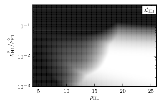
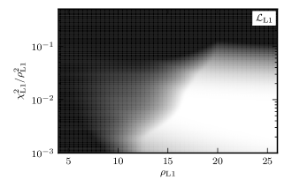
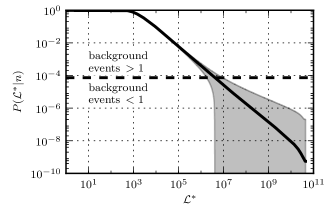
In Fig. 1 we show some of the intermediate data used in estimating the significance of events in our example. Namely, we show the individual likelihood contours for and described in (1) in the H1 and L1 instruments for signals with a chirp mass consistent with a neutron star binary () in Subfig. 1 and 1 respectively. The probability of getting an event with a likelihood greater than after trials for the H1 and L1 instruments (13) is shown in Fig. 1. Our ability to measure is limited by the number of events that we collect in our background estimate. The shaded region shows the error region found by assuming Poisson errors on the number of events that went into computing a given point on the curve. We have indicated the FAP at which there ceases to be more than 1 event collected in the background by a dashed line. The dashed line shows the has background events to which is nearly the FAP required for a detection. Below the dashed line the FAP estimate is dominated by the Gaussian smoothing kernel applied to the planes in Figs. 1 and 1. We believe that it is reasonable to trust the FAP estimate beyond the single background event limit but note that level confidence can still be reached without extrapolation with tighter coincidence criteria. Tighter coincidence criteria would reduce the trials factor and permit higher significances to be estimated. The best way to do this is to demand that three or more detectors see an event. In our example a third detector would lower the trials factor by , which would shift the limiting FAP, to . It is worth mentioning that the background events and number of independent trials are accumulated at the same rate. Thus one cannot decrease the limiting FAP by collecting more data.
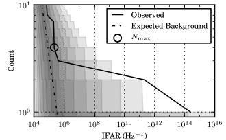
After assigning the FAP to events we also assign a FAR according to (10). This allows us to produce the standard IFAR plot commonly produced in recent searches for compact binaries CBC:S51yr ; CBC:S6 without having relied on time shifting the detector events to estimate the background. This is shown in Fig. 2.
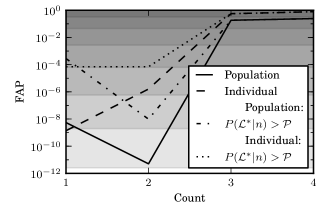
The IFARs of the most significant events that came out of this search in Fig. 2 can be identified as the long tail in the observed events distribution. The top event has a significance greater than , the level necessary for claiming the detection of GWs. The second loudest event has a significance greater than . Both events surpass the single background event limit . If restricted to this limit then both events are nearly .
Applying the population procedure we have put forth in Sec. III, we produced a more significant statement about the presence of GWs beyond that of the loudest event. This effect is mostly attributed to the similar significance of the top two events. This could happen in a real analysis in two ways 1) Nature could just provide such a set of events as in this example 2) both events exhaust our ability to measure significance and we must place an upper bound on the FAP. The latter case, although somewhat artificial, could still play an important role in analysis, especially if one is unable to confidently declare a single event but finds two or more events with 3 or . With our example analysis the combination of the two loudest events was a excursion even after restricting the FAP of both events to be . After examining the signal population we found that both candidates were separately associated with signal injections.
V Conclusion
We have provided a method for estimating the significance of GWs from compact binary coalescence using measurements of single instrument populations of and as a function of the template waveform intrinsic parameters. We demonstrated our method with mock Advanced LIGO data derived from initial LIGO data including a realistic population of compact binary merger signals and glitches. We found that between our two loudest events we were able to establish detection at greater than confidence. Both of the loudest two events exhausted the () background estimate, but the extrapolated FAP of the loudest event exceeded on its own. Both of the loudest events were associated with the blind signal population introduced into the data and the remaining events were consistent with the expectation from background.
Acknowledgements.
Research at Perimeter Institute is supported through Industry Canada and by the Province of Ontario through the Ministry of Research & Innovation. KC was supported by the National Science and Engineering Research Council, Canada. DK was supported from the Max Planck Gesellschaft. This work has LIGO document number LIGO-P1200031. The authors wish to thank Rahul Biswas, Patrick Brady, Gabriela González Jordi Burguet-Castell, Sarah Caudill and Ruslan Vaulin for many fruitful discussions. The authors also thank John Whelan for a careful review of this work. We thank the UW-Milwaukee Center for Gravitation and Cosmology and the LIGO Laboratory for use of its computing facility to make this work possible through NSF grants PHY-0923409 and PHY-0600953. We thank the LIGO Scientific Collaboration and the Virgo Scientific Collaboration for providing us with the data to test the methods described in this work.Appendix A Numerical Considerations
A.1 Equation (8)
As the duration of the experiment increases, the numerical evaluation of (8) using fixed-precision floating point numbers becomes challenging. In this limit, the per-trial false-alarm probability of interesting events is very small and the number of trials is very large. Using double-precision floating-point numbers, when the number of trials gets larger than about , FAPs of and 0 become indistinguishable, and as the number of coincidences that are recorded increases further “4” and “5” events cannot be differentiated — it is no longer possible to make detection claims. The following procedure can be used to evaluate (8) for all and . If the Taylor expansion of (8) about converges quickly.
| (14) |
The last form yields a recursion relation allowing subsequent terms in the series to be computed without explicit evaluation of the numerator and denominator separately (which, otherwise, would quickly overflow): if the term is , the term in the series is .
If the Taylor series still converges (infact, as long as the number of trials is an integer the series is exact in a finite number of terms) but the series is numerically unstable: the terms alternate sign and one must rely on careful cancellation of large numbers to obtain an accurate result. In this regime the expression’s value is close to 1, so is small. If is small, we can write
| (15a) | |||
| and then the Taylor expansion of about converges quickly, | |||
| (15b) | |||
Altogether, the algorithm for evaluating (8) is: if use (14) computed via the recursion relation; otherwise if use (15); otherwise evaluate (8) directly using normal floating point operations. The threshold of for using (15) is found empirically, the results are not sensitive to the choice of this number.
A.2 Equation (10)
The evaluation of (10) for events that are interesting as detection candidates after an experiment is concluded is straight-forward using double-precision floating-point arithmetic. In this regime, , and there is plenty of numerical dynamic range available. However, the practical use of (10) is in its ability to identify “once a day” or “once an hour” events for the purpose of providing alerts to the transient astronomy community. After just one day, 24 “once an hour” background events are expected, and their FAP — the probability of observing at least one such event from a Poisson process you expect to have produced 24 — is 0.9999999999622486. After 37 events are expected, double-precision numbers can no longer be used to differentiate those events’ FAPs from 1; that is, (10) can only assign reliable false-alarm rates to the 30 or so most significant background events in any experiment.
This problem is addressed by not computing the expected number of events, , from the false-alarm probability, , as shown in (10), but by first going back and rewriting (7) and (8) as
| (16) |
from which we can rewrite (10) as
| (17) |
This form of the expression presents no challenges to its evaluation using double-precision floating point arithmetic.
References
- (1) J. Abadie et al. (The LIGO Scientific Collaboration), Class. Quantum Grav. 27, 173001 (2010)
- (2) J. Slutsky, L. Blackburn, D. A. Brown, L. Cadonati, J. Cain, M. Cavaglià, S. Chatterji, N. Christensen, M. Coughlin, S. Desai, G. González, T. Isogai, E. Katsavounidis, B. Rankins, T. Reed, K. Riles, P. Shawhan, J. R. Smith, N. Zotov, and J. Zweizig, Class. Quantum Grav. 27, 165023 (2010)
- (3) B. Abbott et al. (The LIGO Scientific Collaboration), Phys. Rev. D 69, 122001 (2004), http://arxiv.org/abs/gr-qc/0308069
- (4) B. Abbott et al. (The LIGO Scientific Collaboration), Phys. Rev. D 72, 082001 (2005), http://arxiv.org/abs/gr-qc/0505041
- (5) B. Abbott et al. (The LIGO Scientific Collaboration), Phys. Rev. D 72, 082002 (2005)
- (6) B. Abbott et al. (The LIGO Scientific Collaboration), Phys. Rev. D 73, 062001 (2006)
- (7) T. L. S. Collaboration and the TAMA Collaboration (The LIGO Scientific Collaboration), Phys. Rev. D 73, 102002 (2006)
- (8) B. Abbott et al. (The LIGO Scientific Collaboration), Phys. Rev. D 78, 042002 (2008)
- (9) B. Abbott et al. (The LIGO Scientific Collaboration), Phys. Rev. D 77, 062002 (2008), http://arxiv.org/abs/0704.3368
- (10) B. Abbott et al. (The LIGO Scientific Collaboration), Phys. Rev. D 79, 122001 (2009), http://arxiv.org/abs/0901.0302
- (11) B. P. Abbott et al. (The LIGO Scientific Collaboration), Phys. Rev. D 80, 047101 (Aug 2009), http://link.aps.org/doi/10.1103/PhysRevD.80.047101
- (12) J. Abadie et al. (The LIGO Scientific Collaboration and The Virgo Collaboration), Phys. Rev. D 82, 102001 (Nov 2010), http://link.aps.org/doi/10.1103/PhysRevD.82.102001
- (13) J. Abadie et al. (The LIGO Scientific Collaboration and The Virgo Collaboration), Phys. Rev. D 83, 122005 (Jun 2011), http://link.aps.org/doi/10.1103/PhysRevD.83.122005
- (14) J. Abadie et al. (The LIGO Scientific Collaboration and The Virgo Collaboration)(2012), http://arxiv.org/abs/1111.7314
- (15) B. A. Allen, W. G. Anderson, P. R. Brady, D. A. Brown, and J. D. E. Creighton(2005), gr-qc/0509116
- (16) B. Allen, Phys. Rev. D 71, 062001 (2005)
- (17) C. Hanna, Searching for gravitational waves from binary systems in non-stationary data, Ph.D. thesis (2008)
- (18) P. Gregory, Bayesian Logical Data Analysis for the Physical Sciences (Cambridge University Press, 2005)
- (19) K. C. Cannon, Class. Quantum Grav. 25, 105024 (2008)
- (20) In practice it can be difficult to know if the coincidences formed are independent, however as long as they are related to the true number of independent trials by an overall scaling, one can adjust the number so that it agrees with the observed rate of coincidences for low significance events. This works because GWs are very rare and true signals will vastly underwhelm the false positives that a pipeline produces at high FAP. Thus the bias in calibrating to high FAP events is very small.
- (21) L. S. Finn, S. D. Mohanty, and J. D. Romano, Phys. Rev. D 60, 121101 (Nov 1999), http://link.aps.org/doi/10.1103/PhysRevD.60.121101
- (22) B. Abbott et al. (The LIGO Scientific Collaboration), Phys. Rev. D 77, 062004 (Mar 2008), http://link.aps.org/doi/10.1103/PhysRevD.77.062004
- (23) B. P. Abbott et al., The Astrophysical Journal 715, 1438 (2010), http://stacks.iop.org/0004-637X/715/i=2/a=1438
- (24) P. Astone, D. Babusci, M. Bassan, P. Carelli, E. Coccia, C. Cosmelli, S. D’Antonio, V. Fafone, F. Frontera, G. Giordano, C. Guidorzi, A. Marini, Y. Minenkov, I. Modena, G. Modestino, A. Moleti, E. Montanari, G. V. Pallottino, G. Pizzella, L. Quintieri, A. Rocchi, F. Ronga, L. Sperandio, R. Terenzi, G. Torrioli, and M. Visco, Phys. Rev. D 71, 042001 (Feb 2005), http://link.aps.org/doi/10.1103/PhysRevD.71.042001
- (25) J. Abadie et al., The Astrophysical Journal 715, 1453 (2010), http://stacks.iop.org/0004-637X/715/i=2/a=1453
- (26) The LIGO Scientific Collaboration, “Advanced LIGO anticipated sensitivity curves,” (2009), https://dcc.ligo.org/cgi-bin/private/DocDB/ShowDocument?docid=T0900288
- (27) Specifically the zero-detuned, high-power noise curve was used
- (28) B. J. Owen, Phys. Rev. D 53, 6749 (1996)
- (29) A. Buonanno, B. Iyer, E. Ochsner, Y. Pan, and B. Sathyaprakash, Phys. Rev. D 80, :084043 (2009)
- (30) K. Cannon, R. Cariou, A. Chapman, M. Crispin-Ortuzar, N. Fotopoulos, M. Frei, C. Hanna, E. Kara, D. Keppel, L. Liao, S. Privitera, A. Searle, L. Singer, and A. Weinstein, The Astrophysical Journal 748, 136 (2012), http://stacks.iop.org/0004-637X/748/i=2/a=136