Vector Field $k$-Means: Clustering Trajectories by Fitting Multiple Vector Fields

Abstract

Scientists study trajectory data to understand trends in movement patterns, such as human mobility for traffic analysis and urban planning. There is a pressing need for scalable and efficient techniques for analyzing this data and discovering the underlying patterns. In this paper, we introduce a novel technique which we call vector-field $k$-means.

The central idea of our approach is to use vector fields to induce a similarity notion between trajectories. Other clustering algorithms seek a representative trajectory that best describes each cluster, much like $k$-means identifies a representative “center” for each cluster. Vector-field $k$-means, on the other hand, recognizes that in all but the simplest examples, no single trajectory adequately describes a cluster. Our approach is based on the premise that movement trends in trajectory data can be modeled as flows within multiple vector fields, and the vector field itself is what defines each of the clusters. We also show how vector-field $k$-means connects techniques for scalar field design on meshes and $k$-means clustering.

We present an algorithm that finds a locally optimal clustering of trajectories into vector fields, and demonstrate how vector-field $k$-means can be used to mine patterns from trajectory data. We present experimental evidence of its effectiveness and efficiency using several datasets, including historical hurricane data, GPS tracks of people and vehicles, and anonymous call records from a large phone company. We compare our results to previous trajectory clustering techniques, and find that our algorithm performs faster in practice than the current state-of-the-art in trajectory clustering, in some examples by a large margin.

1 Introduction

For many years, scientists have gathered and studied trajectory data to understand trends in movement patterns. Ecologists study animal movements to learn about population growth, social interactions, as well as feeding and migratory patterns [11, 18]. Biologists and computer scientists study the spread of biological and electronic viruses [16, 24]. Meteorologists use trajectory data to help predict storm paths [15, 12, 13], and researchers from a wide variety of fields study human mobility to perform targeted advertising, predict traffic and commuting patterns, and data-driven urban planning [9, 8].

The recent ubiquity of GPS and RFID devices has caused a rapid increase in the amount of available trajectory data. These devices have been used to determine locations of animals, shipping containers and different vehicles. Even in the absence of explicit tracking devices, crowdsourcing can be used as an alternative to gather similar data [18], although with considerable labor requirements. Another option involves looking at cellular phone handoff patterns: the traces of calls as they are handed from one cellphone tower to another [10, 35, 8]. This approach can greatly simplify and automate the data acquisition while still providing complete anonymity for individuals. In all such cases, due to the vast amount of data being collected, there is a great need for scalable and efficient techniques for analyzing this data and discovering the underlying patterns [20].

The analysis of this kind of data is challenging not only because of its size, but also due to its complexity [36]. Trajectories are spatio-temporal in nature, involving geometric positions, directions, velocities, durations, life spans, and potentially many other characteristics specific to the entities being tracked. Hurricane tracks may include overall storm strength, wind speeds, or seasonality. Animal tracks may be influenced by their size, age, or gender. The same attributes can be included for human mobility, as well as their mode of transportation. Incorporating these characteristics, when available, can help direct the trajectory analysis, but also adds complexity. Gudmundsson et al. [20] suggest that it may be possible to infer the characteristics simply by looking at the trajectory data itself.

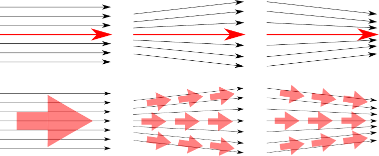
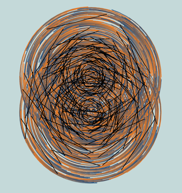
In this work, we present a model-based trajectory clustering approach that uses vector fields as the models for the clustering. Our method, called vector field $k$-means, consists of finding vector fields whose integral lines approximate the given trajectory dataset. The use of vector fields allows us to naturally encode features of the trajectories such as direction and speed, which has not been achieved by previous techniques that used either distance metrics between trajectories or density-based methods ([20, 25]). Our modelling also has the advantage of producing a simple and physically reasonable modelling. This is obviously useful when dealing with datasets representing natural phenomena like storm tracks (see expermiental restults in Section 5.2); however, we also show that this approach can successfully mine human mobility patterns from GPS coordinates and even from extremely noisy datasets such as call detail records (Sections 5.3 and 5.4). Furthermore, vector fields are a good summary for trajectory clusters and can be easily visualized using any of the numerous techniques available from the vast literature on vector field visualization. Previous clustering methods use “representative” trajectories as a way to summarize the result of the clustering process [25], but this is not enough to show all the possible variability inside a cluster, as demonstrated in Fig. 1 (see also Section 5).

One final argument for clustering a set of trajectories using our method is its innate capability of handling partially collected or missing data, a problem that, to the best of our knowledge, has not been addressed in the literature. In many situations, it is not possible to track an entity, thereby generating its trajectory, throughout its entire lifetime. For example, in the case of visually tracking migratory birds, our access might be limited to a very short time frame. As presented in Section 5.4, some data, such as call detail records, can only be used in an anonymous fashion for privacy reasons. In this case, a trajectory can only be inferred by the cell tower handoff during an active call and there is no id that links calls from the same individual. Since users spend most of their time not making calls, tracks are necessarily partial. Clustering methods which use representative trajectories to reconstruct overall patterns will have to resort to stitching [25]. We argue that the technique we develop here is more natural, and we provide experimental evidence that it scales favorably.

For computational efficiency, we use linear approximations of the trajectories and piecewise linear vector fields as models. This allows us, as we show in Section 4, to define the trajectory clustering problem as a (constrained) quadratic minimization problem, that surprisingly connects techniques from scalar field design on meshes [40, 41] and $k$-means clustering. This results in a very easy to implement and efficient algorithm, as we demonstrate with several experimental results. We also compare our algorithm with state-of-the art trajectory clustering algorithms. In summary, our contributions are:

Figure 1: Comparison of summarization of a trajectory dataset using representative trajectories and vector fields. In the top row, different datasets (black) are summarized by the same (red) trajectory, so no variability of the data is captured by the summary. In the bottom row, the same datasets are summarized using vector fields. Notice how this method can better represent the trajectories in the datasets.

• A novel model-based trajectory clustering method based on vector fields, called vector field $k$-means, which gives both a partition of trajectories into meaningful clusters and a best-fitting vector field for each of them.

• An experimental analysis of vector field $k$-means through a collection of datasets of increasingly large scale, together with a discussion and comparison of the results within the context of the current state-of-the-art.

In the following sections, we review related work, introduce the vector field $k$-means technique and show how it can be used in the analysis of trajectory data. We present experimental evidence of its effectiveness using several data sets, including comparisons to previous methods. In both synthetic and real trajectory data, our method can discover significant movement patterns.

Figure 2: An illustration of vector field $k$-means as it partitions 2000 synthetic trajectories into two clusters. The algorithm alternates between fitting the best possible vector fields from the current assignment (“optimize”) and matching trajectories to the vector field which fits them best (“assign”). As we show in Section 4, this procedure always converges. In Section 5, we show that the partitions and the vector fields generated by vector field $k$-means encode useful trajectory patterns. Note that although no individual trajectories form a complete circle, vector field $k$-means still recovers the two separate circular patterns. The vector fields used in this experiment are linearly interpolated over a regular 3x3 grid. Our current implementation of the algorithm converged in 30 iterations on this dataset in about 2 seconds.

2 Related Work

Due to the growing rate at which mobility data is being collected, computational movement analysis is becoming a very active research field, combining techniques and expertise from many other fields, including GIS, information visualization, computational geometry, databases, and data mining [20]. In this work, we focus on just one of the problems in movement analysis, that of extracting arbitrary movement patterns from trajectory data. In other words, given a large number of trajectories of moving objects, e.g. animals, people, or vehicles, we want to quickly identify underlying patterns that exist and that shed light on the global movement trends of the moving objects. As previously described, scientists from many fields can derive immediate benefits from such trends [11, 24, 15]. Our approach for identifying these patterns is to perform trajectory clustering. As Kisilevich et al. [23] provide a thorough examination of many trajectory clustering techniques, we briefly review the most relevant methods here.

Rinzivillo et al. [36] designed a progressive clustering technique that can utilize different distance functions at each step of their clustering. This allows analysis of objects with heterogeneous properties to be handled differently during the cluster refinement stages. Their clustering algorithm is density-based, which is robust to noise and outliers, a common problem with trajectory data. The entire process is visually driven, and interpreting the (quality of the) clusters involves a human analyst. Lee et al. [25] also use density-based clustering, but believe that clustering whole trajectories may miss common sub-trajectories. Therefore, they have created the partition-and-group framework, where they partition the trajectories into line segments based on a simplification algorithm and cluster these segments using the notions of neighborhood and density. These algorithms consider trajectories as a set and do not consider the parametrization of the trajectory and hence they cannot consider information about the speed in their model. Both methods [36, 25] rely on the definition of a distance measure between trajectories (or simplified versions of trajectories such as line segments) which is known to be a difficult problem in the sense that no proposed distance measure captures well all the attributes of trajectories [20]. For example, neither of these methods use timing information for clustering, they only use the geometry of the trajectory and therefore they cannot enconde speed information what might be relevant in cases like storm track analysis. Pelekis et al. [33] exploit local similarities of subtrajectories too, but they also study the effect of uncertainty, e.g. in sampling or in measurement, in the original trajectory data.

Like Rinzivillo et al., our overall approach falls within the broader category of visual and exploratory movement analysis, which exploits humans’ ability to visually detect patterns, and then steer the visualization and analysis to those regions of greatest interest. Andrienko and Andrienko [5, 36, 4] have lead the field in this area. Their work has focused on human-in-the-loop analysis systems, but has also included more general aggregation and visualization of movement data [2], and most recently the identification of important locations and events by analyzing movement data [3, 6].

Liu et al. [26] also present a visual analytics system for exploring route diversity within a city, based on thousands of taxi trajectories. Their system offers global views of all trajectories, but also drills down to routes between source/destination pairs, and even to specific road segments. Their work is more about examining trajectories and less about clustering them.

An important problem related to trajectory clustering is how to ultimately visualize trajectory data. Traditionally flow maps [34, 44, 6] have been used to convey the amount of people and goods that moved between locations but without necessarily reporting the exact routes that were taken. More recently, there have been several compelling techniques based on density maps [47, 38, 37], and kernel density estimation [14].

Vector fields have been widely used in scientific visualization and even by some researchers doing trajectory clustering analysis to show speed and direction of animal movements [11] and wind [13]. In these cases, they have only been used to visualize the results, rather than as an integral part of the underlying clustering technique.

One important class of clustering frameworks is the model-based clustering approach in which our method is included. The algorithms in this class will typically define a generative model for the trajectories and then use Maximum Likelihood estimation to fit the model with the given data. An important feature of these algorithms is that it they produce interpretable models for each cluster. One example of this approach is the work by Gaffney and Smyth [19], in which they used regression mixture models to find their clusters. A similar idea was used by Wei et al. [46] in which they used polynomials as models for the trajecotries.

The idea of using vector fields as tools to analyze trajectory data was previously used in the image processing community [29, 28], but these works used a probabilistic generative model for trajectory datasets using vector field in which a trajectory can be generated by different clusters, which can be hard for an analyst. In our work, we take a geometric approach to the problem with no probabilistic assumptions on the data. As discussed in more details later, our approach conceptualizes the input data set as composed of streamlines of a certain number of vector fields. We approximate this by considering only piecewise linear vector fields, which enables us to define the Vector Field $k$-means algorithm on a least squares optimization that follows the same pattern as the one proposed in the geometry processing community for triangle mesh optimization [40, 41, 30].

Figure 3: This figure illustrates the tessellation of the trajectories, so each segment is contained on a face of the grid. The points with odd indices, where the original trajectories cross face edges, are added in the beginning of the algorithm. In this case each segment of the trajectory determines a constraint in the form of a matrix $C$.

3 Vector Field K-Means

In this section we give a high-level overview of the vector field $k$-means technique. We start by setting the terminology to be used in the rest of the paper.

3.1 Terminology

Trajectories are modeled as paths of the form $\alpha:[t_{0},t_{1}]\rightarrow\mathbb{R}^{2}$. We assume we are given a set of $n$ trajectories $\mathcal{T}=\{\alpha_{1},...,\alpha_{n}\}$. Trajectories are given as samples, i.e., for each $i=1,...,n$, we are given a sequence of space-time points $\widehat{\alpha_{i}}=\{(\alpha_{i}(t^{i}_{1}),t^{i}_{1}),(\alpha_{i}(t^{i}_{2}),t^{i}_{2}),\ldots,(\alpha_{i}(t^{i}_{p_{i}}),t^{i}_{p_{i}})\}$. We approximate each trajectory $\alpha_{i}$ with piecewise linear curves (constant velocity between two consecutive samples). This results in a polygonal line representation for each trajectory. For each $\alpha_{i}$ we denote the interval $[t^{i}_{1},t^{i}_{p_{i}}]$ by $I_{i}$ and by $|I_{i}|$ the timespan for $\alpha_{i}$, i.e., $|I_{i}|=t^{i}_{p_{i}}-t^{i}_{1}$. We call each portion of trajectory between two samples as a segment of the trajectory $\alpha_{i}$. For each segment $s_{j}=[\alpha_{i}(t_{j}),\alpha_{i}(t_{j+1})]$ of $\alpha_{i}$ we define $\omega_{s_{j}}=\frac{t_{j+1}-t_{j}}{T}$, where $T=\sum\limits_{\alpha_{i}\in\mathcal{T}}|I_{i}|$ is the total time span in the dataset.

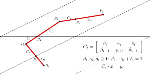
In this paper, our vector fields are always steady and defined on a domain $\Omega\subset\mathbb{R}^{2}$, i.e. they are functions $X:\Omega\rightarrow\mathbb{R}^{2}$. We discretize $\Omega$ as a regular grid $G$ with resolution $R$ ($R^{2}$ vertices) and assume linear interpolation within each face of the grid for the reconstruction of the vector field. We assume that all given trajectories are contained in the domain of interest, and also we assume that all the trajectories are tesselated by the grid so that each trajectory is comprised of segments (portions of the curve between two consecutive vertices) that do not cross the boundaries of the domain triangles as in Fig. 3. Finally, for each segment $s$ of a trajectory $\alpha$ we denote by $C_{s}$ the $2\times R^{2}$ matrix that contains in the first and second row respectively the baricentric coordinates of the first and second vertex of the segment (it has 0 in the entries corresponding to vertices not contained in the face where the segment $s$ lies), Fig. 3 illustrates the setting.

3.2 Method

Our ultimate goal is to mine movement patterns within large trajectory datasets. Our approach is to capture those patterns by defining a vector field for which the trajectories are approximately integral lines, according to a reasonable error measure. However, any non-trivial dataset is likely to contain trajectories that cannot be modeled as streamlines of a single vector field. We use this fact to define a similarity notion between trajectories, namely how well these trajectories can approximate streamlines of a single vector field. We then propose using this similarity to find multiple vector fields that capture the movement features of the dataset under consideration. Vector field $k$-means attempts to separate the trajectories into a small number of clusters according to the best vector field that approximates them.

More formally, the basic assumption of our approach is that for every set of trajectories $\mathcal{T}$, there exists a set of reasonably smooth vector fields $X_{i}\in F,|F|=k$ that explains most of the mobility in the data, in the sense that each trajectory would be approximately tangent to one of the $X_{i}$. As discussed in the previous paragraph, in general we must have $k>1$. Therefore we see each vector field not only as a summary of the trajectory cluster, but also as the center of the cluster, and thus analogous to the original $k$-means algorithm [27].

The problem then is to (1) define these vector fields and (2) assign each trajectory to the vector field that fits it best. In other words, we need to compute both the best-fitting vector fields and a function $\Phi:\mathcal{T}\to\{1,2,\cdots,k\}$ which assigns the trajectories to the best vector field. We propose to look for reasonably smooth vector fields that are approximately tangent to the trajectories. We propose an iterative process that uses the results of step (2) in order to perform step (1) and conversely uses results from step (2) to perform step (1). More clearly, the Vector field $k$-means algorithm consists of the following two steps

• Given any candidate assignment of trajectories $\Phi$, for each set $\Phi^{-1}(i),$ $i=1,\ldots,k$, we find the best-fitting vector fields over those particular trajectories, and

• Given a set of vector fields $\tilde{V}=\{X_{1},\ldots,X_{k}\}$, in order to compute the best assignment function for those particular vector fields we simply evaluate the error (defined later) over each vector field, and pick the best field for each trajectory.

Algorithm 1 contains the outline of the Vector field $k$-means algorithm. In this pseudo-code, the step $(*)$ corresponds to the $fitVectorField$ routine and as we will show below, we can formulate this step as a linear system whose solution can be computed essentially in linear time, and which gives us the smoothest, best-fitting vector field for a set of trajectories. As mentioned earlier, this system has the same general form as the ones proposed by [40, 41, 30] for polygonal mesh processing. The step $(**)$ corresponds to finding the vector field with smallest error with respect to a given trajectory. The error measure $E$ is going to be defined later. We highlight that although vector field $k$-means follows the same lines of the ordinary $k$-means [27] algorithm, they are fundamentally different in the sense that the cluster “centers” are objects of a different nature than the objects being clustered.

Figure 4: This figure illustrates the computation of the Laplacian matrix that we use as a smoothness penalty, to favor simpler vector fields over more complicated ones.

The execution of vector field $k$-means on a synthetic dataset with 2000 overlapping trajectories is illustrated in Fig. 2. In each iteration of the algorithm, the two clusters of trajectories and their corresponding vector fields are improved until a perfect separation occurs at iteration 30. Section 4 explains the algorithm in detail.

Algorithm 1 Vector Field K-Means Outline

0:  $k$: Number of clusters, $\mathcal{T}=\{\alpha_{1},\ldots,\alpha_{n}\}$: Array of curves

0:  $V=\{X_{1},\ldots,X_{k}\}$, $\Phi:\mathcal{T}\rightarrow\{1,\ldots,k\}$

  $\Phi\leftarrow$ Initialize($\mathcal{T}$,$k$)

  repeat

     for $i=1$ to $k$ do

        $f_{i}\leftarrow$ $\textrm{fitVectorField}(\Phi^{-1}(i))$

     end for

     for $i=1$ to $n$ do

        $j_{0}\leftarrow\underset{j\in\{1,2,...,k\}}{\operatorname{argmin}}E(X_{j},Curves(i))$

        $\Phi(\alpha_{i})\leftarrow j_{0}$

     end for

  until not converge

4 Algorithm

In this section we describe the algorithm in detail. Vector field $k$-means finds a minimum of the following energy:

$$E=\underset{X_{j},\Phi}{\min}\,\lambda_{L}\sum_{j=1}^{k}\left|\left|\Delta X_{j}\right|\right|^{2}+\sum_{\alpha_{i}\in\Phi^{-1}(j)}\int_{t^{i}_{1}}^{t^{i}_{p_{i}}}\left|\left|f(\alpha_{i}(t))-\alpha_{i}^{\prime}(t)\right|\right|^{2}\,dt$$ (1)

This energy is always non-negative. As we will show, each iteration of vector field $k$-means reduces E, and since there’s only a finite number of assignments, vector field $k$-means is guaranteed to terminate. In equation 1, $\lambda_{L}$ plays the role of a weighting factor: if close to $0$, we are giving relatively high priority to the trajectory constraints through the matrices $C_{s}$. When it is close to $1$, solutions will tend to be smoother, since most of the energy is spent minimizing $\sum_{i}||\Delta X_{i}||^{2}$.

4.1 Fitting Vector Fields

The $fitVectorField$ routine is the central step of vector field $k$-means. It consists of an optimization problem with two types of constraints: value and smoothness, defined below. As depicted in Algorithm 1, in this step we are given a subset $\mathcal{T^{\prime}}$ of $\mathcal{T}$. We formulate the vector field fitting problem as a lest-squares minimization problem. To simplify our discussion, we consider only a single trajectory $\alpha_{i}\in\mathcal{T^{\prime}}$ and show how to build the optimization problem for it. We then formulate the problem for the entire set $\mathcal{T^{\prime}}$ by simply putting together the constraints for the different trajectories in $\mathcal{T^{\prime}}$. We want to get a vector field for which the trajectory $\alpha_{i}$ is (approximately) a integral line, i.e., we must have $X(\alpha_{i}(t))=\alpha_{i}^{\prime}(t)$. We see each $t\in I_{i}$ as a contraint to the value of $X$. In our discrete setting, given $\alpha_{i}(t)$ we denote by $C_{\alpha_{i}(t)}X$ the line vector indexed by the vertices of the grid containing the baricentric coordinates of $\alpha_{i}(t)$ (it has 0 in the entries not contained in the face where $\alpha_{i}(t)$ lies). The constraint equation just mentioned becomes $C_{\alpha_{i}(t)}X=\alpha_{i}^{\prime}(t)$.

4.1.1 Value Constraints: from discrete to continuous constraints

We have infinitely many such constraints, so we cannot directly write the constraints for all the points on $\alpha_{i}$. In this section we show that we can write all this contraints in a matricial form on the segments of $\alpha_{i}$. Consider each segment $s$ of $\alpha$ and denote by $C_{s}$ the ($2\times R^{2}$) matrix containing the baricentric coordinates of the endpoints of $s$. Furthermore consider the ($m+1\times 2$) matrix $\Lambda_{m}$:

$$\Lambda_{m}=\frac{1}{\sqrt{m}}\left(\begin{array}[]{cc}1&0\\ 1-1/m&1/m\\ \vdots\\ 1/m&1-1/m\\ 0&1\end{array}\right).$$

Consider the equation $\Lambda_{m}C_{s}x=\Lambda_{m}\alpha^{\prime}_{s}$, where $\alpha^{\prime}_{s}$ denotes the vector containing the velocity vectors of $\alpha$ at the endpoints of $s$. This equation simply represents the process of sampling $m+1$ equally spaced points on the segment $s$ and writing down the constraints as discussed in the previous section. More clearly, if $m=1$, we simply have that $\Lambda_{1}$ is the identity matrix and the matrices $\Lambda_{m}C_{s}$ introduce only endpoint constraints. If $n=2$, on the other hand, we would have constraints not only on the endpoints but on the midpoint of the segment as well. The normalization factor $\frac{1}{\sqrt{m}}$ keeps the total weight of this constraint the same as $m$ grows. By increasing $m$, we set constraints over progressively larger sets of points on each segment. We are interested in the case where $m$ grows without bounds. Although we appear to have an arbitrarily large $\Lambda_{m}$ matrix and hence an arbitrarily large number of constraints, the matrix $\Lambda_{m}$ only appears in the normal equations of the least squares problem, and so is always multiplied by its own transpose. In that case, $\Lambda_{m}^{T}\Lambda_{m}$ is always a $2\times 2$ matrix, and so we can define the matrix $\Lambda$ to be the positive-definite square root of the following limit:

$$\Lambda^{T}\Lambda = \lim_{n\to\infty}\Lambda_{n}^{T}\Lambda^{n}$$

$$\Lambda = \left(\begin{array}[]{cc}\frac{1}{2}\left(\frac{1}{\sqrt{2}}+\frac{1}{\sqrt{6}}\right)&\frac{1}{2}\left(\frac{1}{\sqrt{2}}-\frac{1}{\sqrt{6}}\right)\\ \frac{1}{2}\left(\frac{1}{\sqrt{2}}-\frac{1}{\sqrt{6}}\right)&\frac{1}{2}\left(\frac{1}{\sqrt{2}}+\frac{1}{\sqrt{6}}\right)\end{array}\right)$$

We then (re)define the value constraints for $\alpha_{i}$ as $\varepsilon(X,\alpha_{i}):=\sum_{s\in\alpha_{i}}\omega_{s}||\Lambda(C_{s}X-\alpha_{i}^{s})||_{2}^{2}$, where $\alpha_{i}^{s^{\prime}}$ denotes the vector containing the velocity vector of $\alpha_{i}$ at the endpoints of $s$. Thus, we get the interesting property that the linear system we solve simultaneously tries to satisfy an infinite number of value constraints, while still working in a finite dimensional setting. Using $\Lambda$, $\varepsilon(X,\alpha_{i})$ is essentially square of the $L^{2}$ norm of the difference between the vector field and the trajectory velocity vector on the trajectory points. In order to see this, we notice that

$$||X\circ\alpha_{i}-\alpha_{i}^{\prime}||_{L^{2}}^{2} = \int_{a}^{b}||X(\alpha_{i}(t))-\alpha_{i}^{\prime}(t)||dt=$$

$$\sum\limits_{j=1}^{n-1}\int_{t_{j}}^{t_{j+1}}||X(\alpha_{i}(t))-\alpha_{i}^{\prime}(t)||_{L^{2}}^{2} = \sum\limits_{j=1}^{n-1}\int_{t_{j}}^{t_{j+1}}||X(\alpha_{i}(t))-\alpha_{i}^{j^{\prime}}||_{L^{2}}^{2},$$

where $\alpha_{i}^{j^{\prime}}$ denotes the velocity vector of the $i^{th}$ segment of $\alpha_{i}$. Therefore,

$$||X\circ\alpha_{i}-\alpha_{i}^{\prime}||_{L^{2}}^{2}=\sum\limits_{j=1}^{n-1}\int_{t_{j}}^{t_{j+1}}||X(\alpha_{i}(t))-\alpha_{i}^{j^{\prime}}||_{L^{2}}^{2}=$$

$$\sum\limits_{j=1}^{n-1}(t_{j+1}-t_{j})\int_{0}^{1}||(1-\sigma)X(\alpha_{i}(t_{j}))+\sigma X(\alpha_{i}(t_{j}))-\alpha_{i}^{j^{\prime}}||^{2}d\sigma=$$

$$\sum\limits_{j=1}^{n-1}(t_{j+1}-t_{j})\int_{0}^{1}||(1-\sigma)(X(\alpha_{i}(t_{j}))-\alpha_{i}^{j^{\prime}})+\sigma(X(\alpha_{i}(t_{j}))-\alpha_{i}^{j^{\prime}})||^{2}d\sigma=$$

$$\sum\limits_{j=1}^{n-1}(t_{j+1}-t_{j})(\frac{1}{3}\left|\left|X(\alpha_{i}(t_{j}))-\alpha_{i}^{j^{\prime}}\right|\right|^{2}+\frac{1}{3}\left|\left|X(\alpha_{i}(t_{j+1}))-\alpha_{i}^{j^{\prime}}\right|\right|^{2}+$$

$$\frac{1}{6}((X(\alpha_{i}(t_{j}))-\alpha_{i}^{j^{\prime}})\cdot(X(\alpha_{i}(t_{j+1}))-\alpha_{i}^{j^{\prime}})))=T\varepsilon(X,\alpha_{i})$$

.

4.1.2 Smoothness Constraint

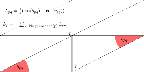
As stated before we also include a smoothness regularity constraint on the vector field. In order to do so we use the the Laplace-Beltrami operator on a vector field. In order to model it, we use the well-known matrix representation of the Laplace-Beltrami operator over polyhedral surfaces and the cotangent formula [45]. In general, if we let $p,q$ be a pair of adjacent vertices of the grid, then the entries of the cotangent Laplacian matrix L are given by

$$\bar{L}_{pq}=\frac{1}{2}(\cot\theta_{pq}+\cot\eta_{pq}),$$

$$\bar{L}_{p}=-\sum\limits_{t\in Neighborhood(p)}\Delta_{pt}.$$

This formula allows us to compute the Laplacian of scalar functions defined over the grid by simply representing the values of the function on the vertices of the grid as a vector and multiplying the vector field by the Laplacian matrix. We illustrate the construction of the Laplacian matrix in Fig. 4.

4.1.3 Fitting Process

We want the vector field $X$ to be defined as the solution of the Laplace equation $LX=0$ (vector Laplacian) with the value constraints defined in the previous section. Therefore, we define the best fitting vector field $X$ for a set of trajectories as the solution (in the least squares sense) of the following system:

$$Lx = 0$$

$$\Lambda C_{s}x = \Lambda y_{s}$$

In the above, $s$ ranges over all segments of the trajectories assigned to the particular vector field. We incorporate the weights on the associated linear system for the normal equations, and solve the following linear system with a unique solution:

$$\left(L^{T}L(\lambda_{L}\sum_{s}\omega_{s})+(1-\lambda_{L})\sum_{s}\omega_{s}(C_{s}^{T}\Lambda^{T}\Lambda C_{s})\right)X=\sum_{s}\omega_{s}(C_{s}^{T}\Lambda^{T}\Lambda y_{s}),$$

where $\lambda_{L}$ is a parameter that idicates the weight of the smoothness penalty in the optimization problem.

Finally we notice that this optimization problem has the same form as the one presented in [40, 41] used in that context for scalar field design on meshes.

4.2 Assigning trajectories to vector fields

In the second phase of the Algorithm 1, we assume we have a fixed set of vector fields $\mathcal{V}=\{X_{1},\ldots,X_{k}\}$ and a set $\mathcal{T}=\{\alpha_{1},...,\alpha_{n}\}$ of trajectories. The goal is to build the next function $\Phi$ that assigns each trajectory to one of the $k$ cluster centers, i.e.the vector fields $X_{1},\ldots,X_{k}$.

The assignment algorithm is trivial: for each vector field $X_{i}$ and trajectory $\alpha$, we simply evaluate

$$\varepsilon(X_{i},\alpha)(1-\lambda_{L})+||LX_{i}||^{2}\lambda_{L}.$$

The new assignment is then the global minimizer of the $k$ possible choices.

dataset	#traj.	res.	$k$	fit	eval	assign
Synthetic	2000	3	2	1.730s	0.076s	0.074s
Atlantic	1415	5	7	8.076s	0.176s	0.335s
Beijing Wide	45563	5	4	110.99s	2.377s	4.265s
Beijing Campus	12883	10	16	124.35s	1.229s	2.195s
CDR	37435	4	4	201.24s	4.227s	7.597s
CDR Large	372601	4	4	2497s	43.127s	75.24s

Figure 5: Experimental results of vector field $k$-means. For each dataset, we report the number of trajectories, the grid resolution (res), the number of clusters (k), and the total running times (in seconds) for the vector field fitting routine, the error evaluations, and the trajectory assignments.

Figure 6: Results of clustering trajectories from the HURDAT dataset [1]. On the left, the original input trajectories are shown. On the right, four trajectory clusters and their corresponding vector fields showing relative speed: the top-left vector field heading northeast is generally faster than the one on the bottom-right . The direction of each trajectory is shown colormapped from blue to orange.

Algorithm 2 Initialization Algorithm

0:  $k$: Number of clusters, $Curves$: Array of curves

0:  $\Phi$: Initial clusters

  $c\leftarrow$ random element from Curves

  $f_{1}\leftarrow$ $\textrm{fitVectorField}(\{c\})$

  for i = 2 to k do

     $c\leftarrow\underset{c^{\prime}\in Curves}{\operatorname{argmax}}\{\underset{\{j|1\leq j<i\}}{\operatorname{min}}E(f_{j},c^{\prime})\}$

     $f_{i}\leftarrow$ $\textrm{fitVectorField}(\{c\})$

  end for

  for i = 1 to Curves.size() do

     $j_{0}\leftarrow\underset{j\in\{1,2,...,k\}}{\operatorname{argmin}}E(f_{j},Curves(i))$

     $\Phi(i)\leftarrow j_{0}$

  end for

4.3 Algorithm Initialization

As with traditional $k$-means, our initialization step has a clear influence on the final results. We implemented a simple method to choose the initial vector fields and trajectory partitions that was effective in our experiments. The main idea is to try to have as diverse initial clusters as possible (see pseudo-code in Algorithm 2). The algorithm takes as inputs an array of curves and a number $k$ of clusters to be created, and starts by choosing a trajectory $\alpha:[t_{0},t_{1}]\to R^{2}$ at random to be part of the first cluster. It uses the $fitVectorField$ routine previously described to fit a single trajectory to the first vector field. The algorithm proceeds by fitting to the $i$-th vector field the trajectory that has the worst error among all previously fit vector fields. After computing $k$ vector fields, we compute the assignment $\Phi$ by picking the best vector fields for each trajectory.

4.4 Computational Complexity and Implementation

As discussed in Section 4.2, the assignment step consists of a linear pass over the trajectory data, and for each of these, we need to find the vector field that minimizes the error (defined in Section 4.2). This can be implemented in $O(k|S(\mathcal{T})|)$, where $S(\mathcal{T})$ denotes the set of line segments that compose the trajectories in $\mathcal{T}$.

For the first step, we have used a simple Unconstrained Conjugate Gradient [39] algorithm as a linear system solver. Therefore, the complexity of this step is given by $O(kN(R^{2}+|S(\mathcal{T})|))$, where $N$ denotes the maximum number of iterations of the Conjugate Gradient Method, $R^{2}$ denotes the grid resolution corresponding to the multiplication by the Laplacian matrix, and $|S(\mathcal{T})|$ corresponds to the multiplication by the constriant matrix $C$. As we see in the experiments good results can be obtained with relative low values of $R$ and hence the complexity is dominated by $kN|S(\mathcal{T})|$. Notice that the algorithm is highly parallelizable (although we did not take advantage of that in our current implementation), the fitVectorField procedure can be executed independently for each cluster.

The choice of the Conjugate Gradients solver was made simply out of convenience; however, we can further optimize our current implementation by using more sophisticated methods to solve systems of linear equations, e.g. Constrained Conjugate Gradients [39] and Cholesky Decomposition [42].

Figure 7: This figure shows about 13000 trajectories from the GeoLife Trajectories dataset clustered using vector field $k$-means. The original trajectories were cropped outside of a small area, and sampled to a 2-minute per-sample resolution. The direction of each individual trajectory is shown colormapped from blue to orange. In the inset, we show the corresponding OpenStreetMap tile for this area of Beijing together with a dendrogram of the clustering. We partition the original data into four clusters, and then partition each cluster a second time, resulting in 16 subclusters. Images (a), (b), and (e) illustrate three of the original clusters together with their corresponding vector fields, while images (c) and (d) show two of the resulting subclusters. Using vector field $k$-means, we can clearly identify movement patterns, including separating faster vehicular (a, b) from slower pedestrian traffic (e).

5 Experiments and Results

We now report the results of running vector field $k$-means. In our experiments, the algorithm was able to efficiently extract significant movement patterns across diverse datasets. We start with a synthetic dataset, and progressively move up to larger examples. Our final result involves clustering over 370,000 very noisy trajectories. All reported running times (see Fig. 5) are from our prototype implementation: a single-threaded, single-process C++ application running on an Intel Core i7-960 desktop with 6GB of RAM. The total amount of memory required by our application remained under 1GB for all reported experiments.

Figure 8: Time (measured in hours since the beginning of the year) and maximum wind speed (miles per hour) distributions for Atlantic hurricanes. Compared to cluster 4, cluster 0 storms tend to happen earlier in the year. Stronger storms appear also more likely to be in cluster 0, although there are few samples in that region. The wide density bands in clusters 2 and 5 are due to outlier storms in strength and maximum wind speed. These attributes are not taken into account for clustering; the features appear simply from the tracks in clusters having related attributes.

5.1 Synthetic Data

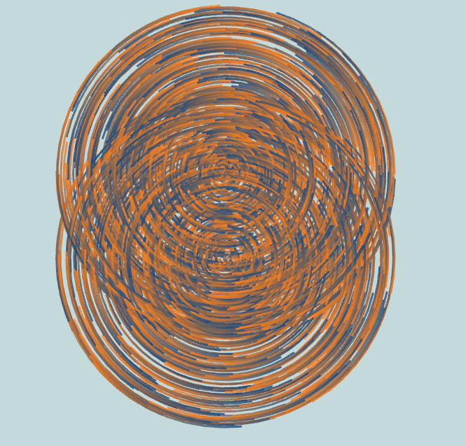
In this synthetic dataset, we assume the existence of two overlapping circulatory movement patterns. Each trajectory covers a partial, randomly selected section of the circle at a random distance from the center. We sample 1,000 trajectories from each overlapping pattern. As we show in Fig. 2, vector field $k$-means recovers the two overlapping patterns perfectly. This shows, very clearly, that vector field $k$-means does not create clusters by selecting representative trajectories at all: its vector fields fit all circular trajectories equally well.

5.2 Atlantic Hurricanes

Figure 9: Large-scale movement patterns around Beijing, GeoLife Trajectories dataset. All but one cluster appear to depict travel in and out of the city from the surrounding highways. The remaining cluster (third from top) has much slower speeds than the other clusters. Its trajectories are also more tightly packed around a small region, and this led us to the experiment shown in Figs. 7 and 10.

HURDAT is a hurricane tracking dataset maintained by the National Hurricane Center (NHC) [1]. The dataset contains 1415 trajectories of different Atlantic storms between the years 1861 and 2011. It contains not only position and time information, but also sustained surface wind speeds, and sea-level pressure information. The data are recorded for every active tropical storm, with a resolution of 6 hours. For the purpose of vector field $k$-means we only need the latitude, longitude, and time of each track.

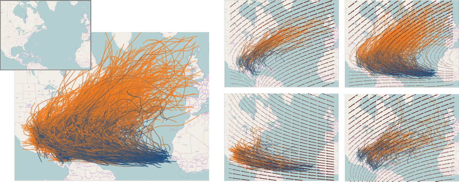
We show four of the seven clusters of our analysis in Fig. 6. Note that vector field $k$-means separates what originally looks like a fairly uniform set of trajectories. One of the clusters neatly capture Cape Verde hurricanes which tend to make landfall in North America, while two separate clusters show hurricanes which originate in the Caribbean and Gulf of Mexico. Upon closer inspection, it appears that this separation of two similar looking trajectory clusters is due to the more chaotic trajectories of one of the clusters, which result in a generally lower-velocity vector field. The remaining cluster has hurricanes with the common trajectory of crossing the Atlantic and moving north-east along the east coast of the United States. The clusters we do not show appear to contain mostly outlier storms, one of which contains 21 hurricanes which move in a northerly fashion.

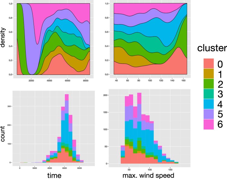
Vector field $k$-means clearly captures the movement patterns of these hurricanes. To assess whether the clusters contain significant other information, we investigated histograms and conditional probability distributions of wind speeds and time of hurricane occurrence, shown in Fig. 8. Attributes that were not taken into account during the clustering are evident when examining the trajectories assigned to each cluster.

5.3 GeoLife GPS Trajectory Dataset

Figure 10: Two of the clusters identified by vector field $k$-means seem to include a particularly repetitive slow trajectory path, which by map inspection we speculate to be a nearby lunch spot for area workers.

The GeoLife GPS dataset consists of a collection of 17,621 trajectories recorded by Microsoft Research at Beijing. The trajectories are GPS tracks of 178 users over a three year period from April 2007 to October 2011 [49, 51, 50]. Although the entire dataset encompasses trajectories throughout the entire planet, in this study we focus on two different regions around Beijing. The raw trajectories from the dataset are unsegmented: some GPS tracks run for days. We split trajectories with the following very simple rule: whenever the time between two samples is larger than 2.5 times the median time between samples, we break off the trajectory. Finally, the dataset is quite densely sampled. We reduce the sampling rate by only keeping measurements at least 2 minutes apart from each other.

Figure 11: In the GeoLife dataset cropped as shown in Fig. 7, different clusters capture different speed features of the trajectory data. The clusters shown here are the first level of the tree, with respectively 2990, 3346, 4209 and 2335 trajectories each. Cluster 2 (named “e” in Fig. 7) has significantly slower trajectories.

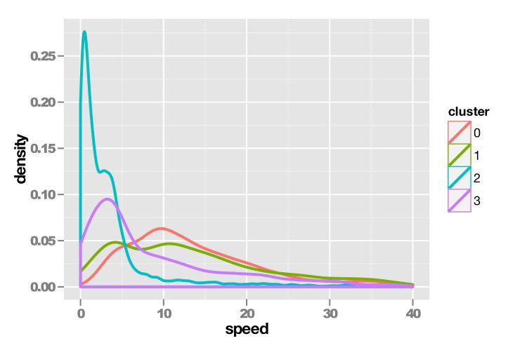
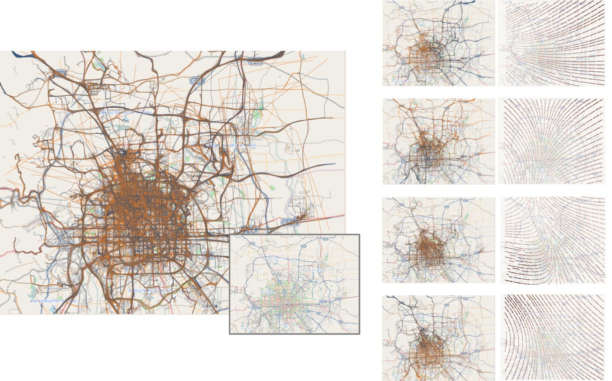
Fig. 9 shows a first run of vector field $k$-means on the GeoLife dataset in which the algorithm was able to find general movement trends within the trajectories. Three of these are clear directional patterns of trajectories heading west, north, and south. We speculate these to be mainly commuting patterns, since the fourth remaining cluster consists essentially of trajectories inside the city’s road network. Although we believe that with the chosen resolution (5x5) vector field $k$-means cannot reliably resolve the patterns in that cluster (and hence the vector field is not very informative), the large density of trajectories around a relatively small area in the cluster suggested to us further analysis centered in that region.

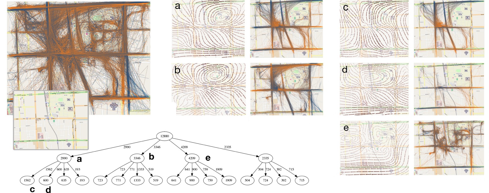
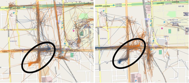
Fig. 7 shows an exploration we performed on that narrower region of Beijing. For that same dataset, Fig. 11 shows the distribution of average speed for the first level of the tree in Fig. 7. Notice that vector field $k$-means is able to separate trajectories not only by their overall movement trend (direction), but also by their speed: cluster (e) clearly contains slower trajectories, which, by examination, seem to be pedestrian traffic. We also notice that cluster (b) contains the fastest trajectories in the database. We found two intriguing patterns in cluster (e): people apparently going to a train station and heading to what seems to be a lunch spot. We highlight this in Fig. 10.

5.4 Call Detail Record Dataset

We collected anonymized Call Detail Records (CDR) from the cellular network of a large US communications service provider. We captured the handoff patterns carried out by approximately 300 cell towers located in the vicinity of Anytown, a suburban city with approximately 20,000 residents. Our goal was to capture handoffs related to vehicular traffic in and around the town.

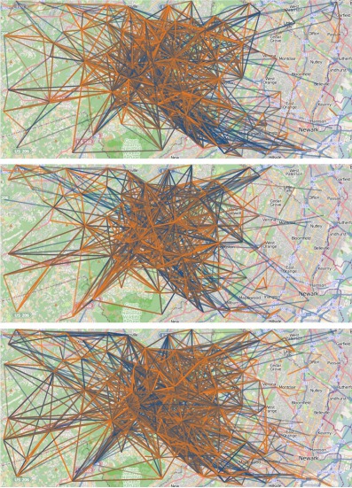
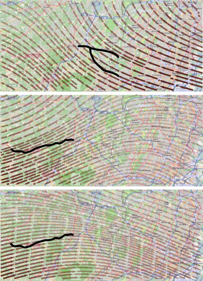
Given the sensitivity of CDR data, we took several steps to ensure the privacy of individuals. The data was collected and anonymized by a third party not involved in the data analysis. Unlike other studies which replace phone numbers by anonymous unique identifiers, we simply have no access to the information [10, 9]. In other words, our dataset cannot associate multiple calls made by the same individuals: each call is completely independent from all the rest. The CDRs contain no information about the second party involved in the call. The only information available is the sequence of antenna locations and handoff times for calls which were handled by more than one physical antenna. Most calls are restricted to a single antenna, so the dataset represents a small fraction of the total calls. In total, we collected over 370,000 calls over the period of a single contiguous week of 2011. As we show in Figs. 16 and 17, although the handoffs are quite noisy, vector field $k$-means can still recover movement patterns clearly related to the highway traffic around the city.

5.5 Comparison

In this Section we compare our algorithm with the TraClus algorithm by Lee et al. [25] As discussed in Section 2 the TraClus algorithm a density based algorithm that has been one of the main references in the area of trajectory clustering. The algorithm consists in two main steps: trajectory simplification in line segments and segment clustering. In the first step each given trajectory are simplified and partitioned in line segments that approximate the input trajecty. The second step consists in clustering the resulting line segments with a DBSCAN like algorithm. The algorithm has essentially 2 parameters: a distance threshold called $\epsilon$ used to define neighborhoods for each segment, and a density lower bound called $MinLns$ that is used to find neighborhoods that define clusters, we refer the reader to the paper [25] for more details. One important Traclus feature is that the time information is not used during the entire process and therefore speed information is lost. For comparisons we use the C++ implementation of the algorithm that is available on the author webpage . In all the following experiments we use the heuristics proposed on the paper (and also part of the author implementation) to select the parameter values and when this heuristics fails to return a value we manually adjusted the parameters using the knowledge of the data set and visual inspection. We highlight that as, explained earlier, vector field $k$-means and TraClus mine different patterns and therefore it is difficult or maybe even impossible to say that one method is better than the other all cases, but we do try to investigate what kind of patterns TraClus is not able to mine that vector field $k$-means and vice versa.

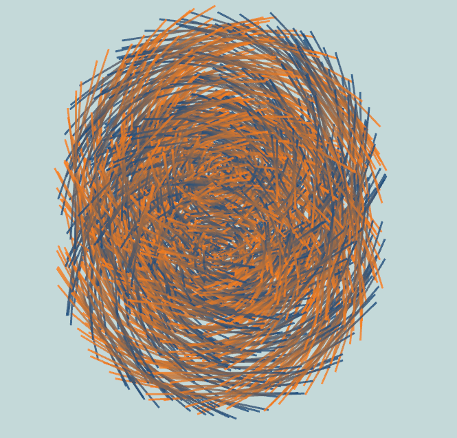
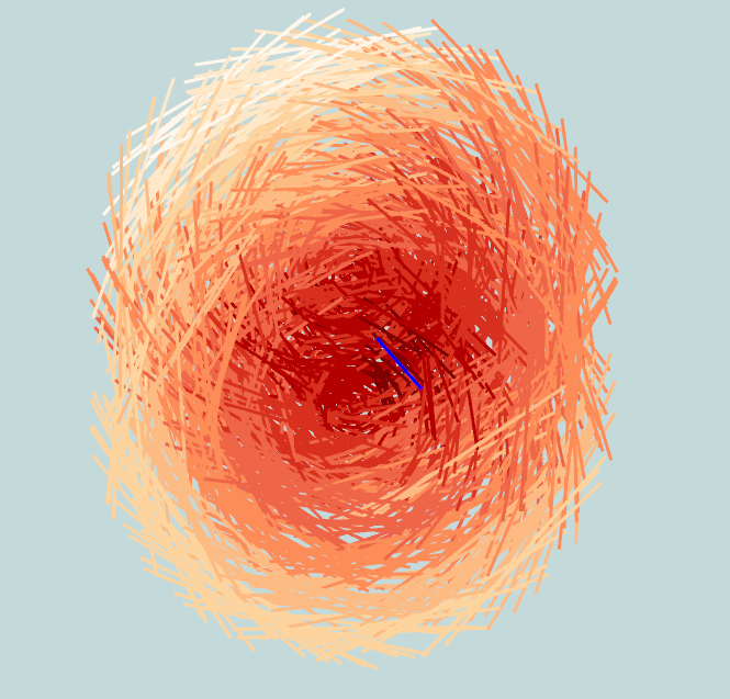
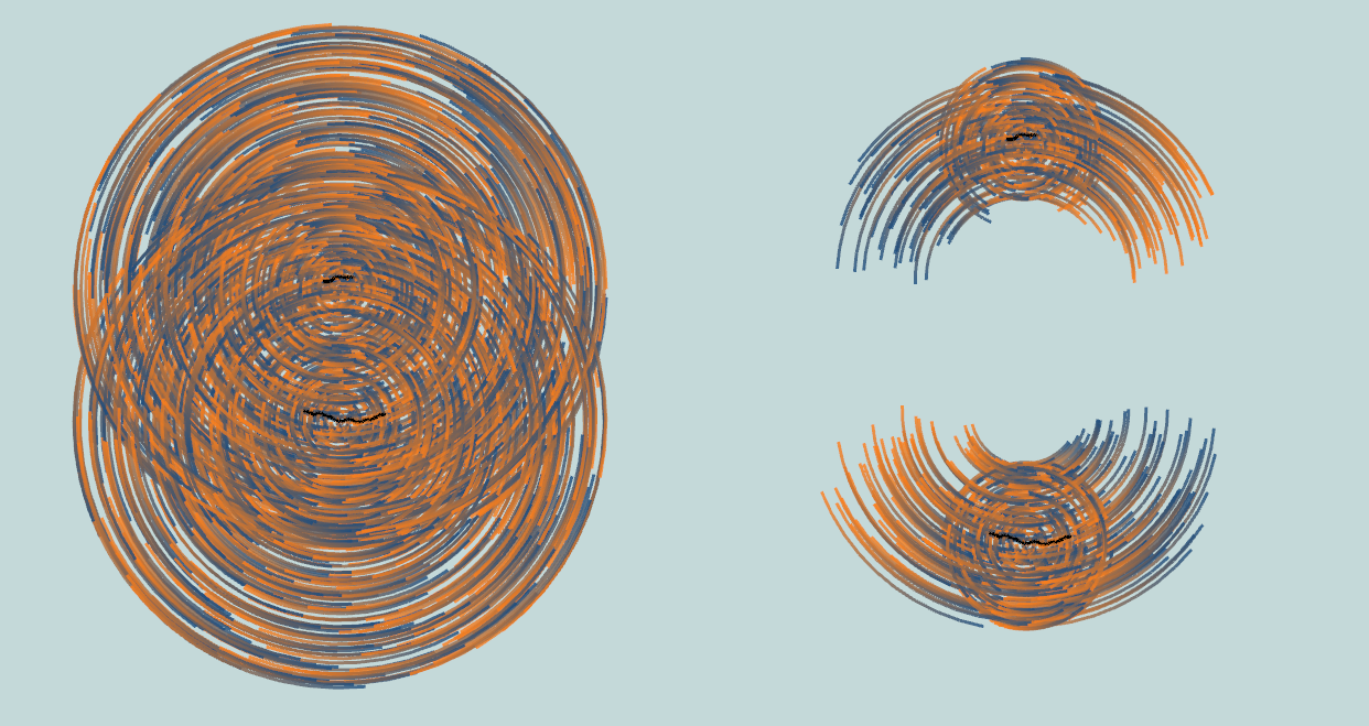
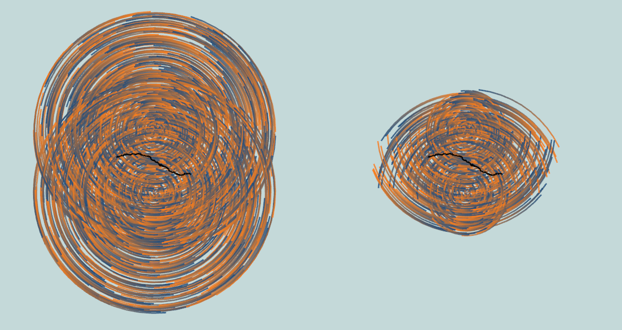
We first present the results of the TraClus algorithm on the synthetic dataset presented in Fig. 2. In Fig. 12 we show the data set used, and in Fig. LABEL:fig:simplified_overview_trajectories the simplified trajectories (result of the first step of TraClus). The idea of investigating this data set is to show that TraClus is not able to separate the center since it looks at local features while as shown in Fig 2 vector field $k$-means is able to capture the global structure by considering the vector fields. When the neighborhood size $\epsilon$ is set to be small, TraClus considers each segment as it’s own cluster, making $\epsilon$ larger by the definition of the metric, the bottom part of the top center is grouped together with trajectories on the bottom center. In this case we get the summarization problem highlighted in Fig.1, in which the mean trajectory is not a good representative of the cluster.We present results of the experiments in Fig 13. We can see that TraClus is unable to separete the two centers.

Figure 12: In (a) we show the input data set and in (b) we show the result of the first step of TraClus. In this case, each trajectory results in exactly one segment (no partition happen). Figure (c) shows the distance measure used by TraClus, the colors show the distances from the blue segment, where darker colors mean smaller distances. We can see that both centers contain close segments to the blue segment and therefore is impossible to completely separete the two centers using TraClus.

Figure 13: This figure illustrates the results of three experiments over the synthetic data set varying the parameters. In (a) the parameters are $\epsilon=0.03$ and $MinLns=2$. In this case 268 are found. Figure (b) shows the results for parameters $\epsilon=0.23$ and $MinLns=140$. In this experiment TraClus is able to detect two cluster, but merges parts of the two centers, basically due to the distance issue mentioned in Fig. 12. A little variation on the parameters ($\epsilon=0.25$ and $MinLns=160$) causes TraClus to merge the two cluster in a single as shown in (c). These results were obtained in 0.8, 1.6, and 6.5 seconds respectively.

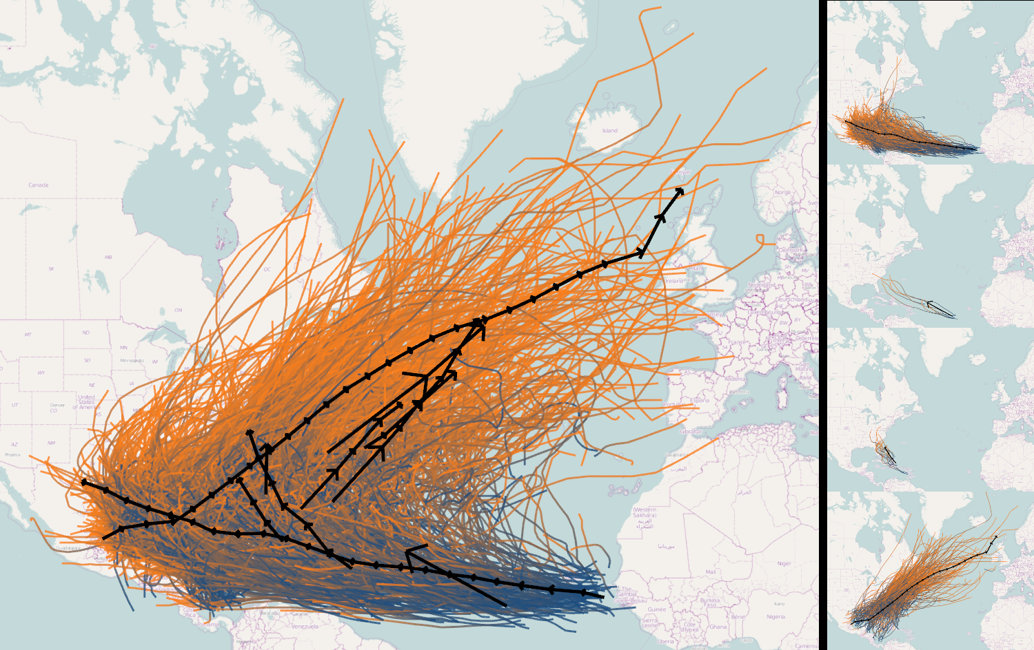
We now experiment with the hurricane data set discussed in Sec. 5.2. Fig. 14 contains the results of TraClus on the hurricane dataset that are similar to the ones obtained by the authors [25], notice that our data set contains more trajectories this is the reason our results are slightly different. By testing a range of parameters, We found that using the same parameters as the ones found by Lee et al. gives us the best results. In this case TraClus detects 10 clusters, as shown on the left of Fig. 14. On the right of Fig. 14 we show the details of some of the clusters. . The results are obtained in 4 seconds.

Figure 14: On the left the nine clusters found. ..

6 Discussion

The algorithm proposed in this paper raises a number of interesting questions, some of which we address in this section. We will also discuss possible extensions of vector field $k$-means in context of its shortcomings or peculiarities.

Figure 15: Increasing the smoothness weight in the optimization is essentially equivalent to decreasing the resolution. Top row, left to right: $R=60$, $\lambda_{L}=[0.05,0.95,0.9995]$. Bottom row, left to right: $\lambda_{L}=0.05$, $R=60,20$, and $5$.

6.1 Dependency on parameters

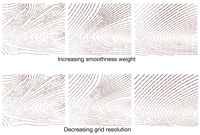
In this section we briefly discuss our experience in how to select the parameters in vector field $k$-means. We note, first of all, that although we can select both grid resolution $R$ and the weight given to the Laplacian regularization $\lambda_{L}$, in practice we never change $\lambda_{L}$, as increasing $\lambda_{L}$ is basically the same as reducing $R$ (see Fig. 15). This happens for a well-known reason: the (orthogonal, unit-length) eigenvectors of the Laplacian are naturally interpreted as equivalent to the fundamental frequencies on the mesh, exactly like sines and cosines are the fundamental frequencies on a circle [43]. The corresponding eigenvalues, on the other hand, are the (squares of) the frequencies themselves. Because of this, as we increase $\lambda_{L}$ we give larger weights to the eigenvectors corresponding to high-frequency signals, and the system tends towards lower-frequency results. At the same time, reducing $R$ directly band-limits the signal on the vector field, which is a quite similar effect. As a result, we set our $\lambda_{L}$ to be $0.05$ in all of our experiments and vary $R$ instead. This has the distinct advantage of generating much smaller linear systems, which can be solved much more quickly.

Picking an appropriate number of clusters remains generally an open problem even in the case of traditional $k$-means, and we offer no substantive contributions on that matter. Many methods proposed in the literature try to attack this problem (for example see [17] and references therein), however no definitive algorithm solves this problem optimally for all aplications in general settings. Still, we stress that as far as performance is concerned, vector field $k$-means compares quite favorably to results reported in the literature. It is much easier to include a human analyst in the loop and make cluster count an interactive procedure with vector field $k$-means than with other methods.

6.2 Advantages

Our proposed model strikes a nice balance between richness and expressivity of features, and simplicity of implementation and analysis. We believe this is a significant advantage over the current methods for trajectory clustering. As mentioned earlier, by representing the cluster centers as vector fields and using those as a means to define similary between trajectories, we can eliminate expensive computations of metrics for trajectories and the computations of the centroid trajectory as well [20]. Vector field $k$-means is also potentially highly parallelizable. Our prototype includes no significant optimizations, but it is obvious that separate components of vector fields can be computed in parallel, and that many of the intermediate matrices in the linear solvers can be reused from one iteration to the next. We expect these to further increase the performance, and allow vector field $k$-means to handle even larger datasets.

6.3 Limitations

Since vector field $k$-means is akin to $k$-means, it inherits the good and bad features from it as well. Still, $k$-means is a very well-studied algorithm and many solutions developed to avoid problems in $k$-means can be adapted to our work with vector field $k$-means. For example, the choice of the initial clusters have a big impact in the results achieved by vector field $k$-means. Many techniques have been proposed to choose good initial centers for the clusters. We highlight the $k$-means++ approach proposed by Arthur et al. [7], which consists of defining the initial centers by randomly choosing the points with probability proportional to the square of the distance between this point and the closest centers already defined. The initialization step used in our implementation of vector field $k$-means (Section 4.3) has no theoretical guarantees, while $k$-means++ gives a $\log k$ approximation to the $k$-means clustering problem. It is an interesting avenue of future work to investigate if the statements about $k$-means++ carry over to vector field $k$-means. Other initialization approaches have also been proposed by Yedla et al. and Patel and Mehta [48, 32]. He et al. offer another general study on possible approaches for cluster initialization [22].

Another issue that happens in $k$-means and also may arise during the execution of the vector field $k$-means is the singularity problem [31]. This occurs when one or more clusters become empty during the computation. This problem is due to bad initialization that may arise in the usual $k$-means and can arise in vector field $k$-means as well. Our current implementation simply repopulates the empty cluster by splitting the largest cluster at that point in the optimization. This is entirely ad-hoc, and we would like a better solution. Again, one could also adapt the methods proposed to avoid this problem for $k$-means to work in vector field $k$-means. Pahkira has some proposal to avoid empty clusters, and points to further references [31].

Figure 16: The anonymized call detail records for over 370,000 cell phone calls produced noisy trajectories (i.e. hand-offs between cell phone towers) around a suburban city. Three of the four clusters computed by vector field $k$-means are shown.

Figure 17: Despite the noisy trajectories, vector field $k$-means is able to recover clear movement patterns related to highway (bold black lines) traffic around the city. The three vector fields correspond to the clusters shown in Fig. 16.

7 Extensions and Future Work

The version of vector field $k$-means presented in this paper derives steady vector fields from trajectory data only. However, it can be generalized to produce time varying vector fields. Fundamentally, this imposes no problems: one simply creates a three-dimensional grid and sets the constraints on the interior of tetrahedral decompositions of a regular grid. It remains to be seen, however, whether the performance characteristics that are so attractive about our current algorithm will remain so in a three-dimensional extension.

For the sake of simplicity, we described the vector field $k$-means algorithm in Section 3 in two dimensions. Nevertheless, we note that vector field $k$-means works with trajectories in any dimension $d$. More precisely, one still could use a variant of the formulation in Equation 1. One would need to involve the region on interest in a simplicial grid of dimension $d$, in which we assume linear interpolation inside each simplex of the grid. Most of the steps would be straightforward to carry through. We note, however, that to the best of our knowledge there is no good three-dimensional equivalent to the cotangent weight of the two-dimensional Laplacian.

Many real-life applications require alignment not only of tangent directions and speed, but also of occurrences in time. Our current algorithm cannot handle these constraints. However, we believe this can be addressed by including a time scalar field as an additional field to be constructed from constraints. From there, the assignment step would simply consider time mismatches as another penalty.

Another interesting research direction worthy of exploring in future work is to apply vector field $k$-means using user input. One could imagine that the user could visually define the vector field or even some sample trajectories and the algorithm would retrieve all trajectories in the database that follow those patterns given by the user, i.e.the ones for which the error relative to the vector field obtained from the trajectories given by the user is small enough.

References

- [1] HURDAT: The national hurricane center’s north atlantic hurricane database, Feb 2012.
- [2] G. Andrienko and N. Andrienko. Spatio-temporal aggregation for visual analysis of movements. In IEEE Symposium on Visual Analytics Science and Technology (VAST), pages 51–58, 2008.
- [3] G. Andrienko, N. Andrienko, C. Hurter, S. Rinzivillo, and S. Wrobel. From movement tracks through events to places: Extracting and characterizing significant places from mobility data. In IEEE Symposium on Visual Analytics Science and Technology (VAST), pages 159–168, 2011.
- [4] G. Andrienko, N. Andrienko, S. Rinzivillo, M. Nanni, D. Pedreschi, and F. Giannotti. Interactive visual clustering of large collections of trajectories. In IEEE Symposium on Visual Analytics Science and Technology (VAST), pages 3–10, 2009.
- [5] G. Andrienko, N. Andrienko, and S. Wrobel. Visual analytics tools for analysis of movement data. SIGKDD Explorations, 9(2):38–46, 2007.
- [6] N. Andrienko and G. Andrienko. Spatial generalization and aggregation of massive movement data. IEEE Transactions on Visualization and Computer Graphics, 17(2):205–219, 2011.
- [7] D. Arthur and S. Vassilvitskii. k-means++: The advantages of careful seeding. In Proceedings of the eighteenth annual ACM-SIAM symposium on Discrete algorithms, pages 1027–1035. Society for Industrial and Applied Mathematics, 2007.
- [8] M.A. Bayir, M. Demirbas, and N. Eagle. Discovering spatiotemporal mobility profiles of cellphone users. In World of Wireless, Mobile and Multimedia Networks & Workshops, 2009. WoWMoM 2009. IEEE International Symposium on a, pages 1–9. IEEE, 2009.
- [9] R.A. Becker, R. Caceres, K. Hanson, J.M. Loh, S. Urbanek, A. Varshavsky, and C. Volinsky. A tale of one city: Using cellular network data for urban planning. IEEE Pervasive Computing, pages 18–26, 2011.
- [10] Richard A. Becker, Ramon Caceres, Karrie Hanson, Ji Meng Loh, Simon Urbanek, Alexander Varshavsky, and Chris Volinsky. Route classification using cellular handoff patterns. In Proceedings of the 13th International Conference on Ubiquitous Computing, pages 123–132, 2011.
- [11] D.R. Brillinger, H.K. Preisler, A.A Ager, and J.G. Kie. An exploratory data analysis (EDA) of the paths of moving animals. Statistical Planning and Inference, 122(2):43–63, 2004.
- [12] S. J. Camargo, A. W. Robertson, S. J. Gaffney, P. Smyth, and M. Ghil. Cluster analysis of typhoon tracks. Part I: General properties. Climate, 20(14):3635–3653, 2007.
- [13] S. J. Camargo, A. W. Robertson, S. J. Gaffney, P. Smyth, and M. Ghil. Cluster analysis of typhoon tracks. Part II: Large-scale circulation and ENSO. Climate, 20(14):3654–3676, 2007.
- [14] O. Daae Lampe and H. Hauser. Interactive visualization of streaming data with kernel density estimation. In Pacific Visualization Symposium (PacificVis), 2011 IEEE, pages 171–178. IEEE, 2011.
- [15] J.B. Elsner. Tracking hurricanes. Bulletin of the American Meteorological Society, 84(3):353–356, 2003.
- [16] S. Eubank, H. Guclu, V. S. A. Kumar, M. V. Marathe, A. Srinivasan, Z. Toroczkai, and N. Wang. Modelling disease outbreaks in realistic urban social networks. Nature, 429:180–184, 2004.
- [17] Yixin Fang and Junhui Wang. Selection of the number of clusters via the bootstrap method. Comput. Stat. Data Anal., 56(3):468–477, March 2012.
- [18] N. Ferreira, L. Lins, D. Fink, S. Kelling, C. Wood, J. Freire, and C. Silva. BirdVis: Visualizing and understanding bird populations. IEEE Transactions on Visualization and Computer Graphics, 17(12):2374–2383, 2011.
- [19] S. Gaffney and P. Smyth. Trajectory clustering with mixtures of regression models. In Proceedings of 5th ACM SIGKDD International Conference on Knowledge Discovery and Data Mining, pages 63–72, 1999.
- [20] J. Gudmundsson, P. Laube, and T. Wolle. Computational movement analysis. Springer Handbook of Geographic Information, pages 725–741, 2012.
- [21] M. Haklay and P. Weber. Openstreetmap: User-generated street maps. Pervasive Computing, IEEE, 7(4):12–18, 2008.
- [22] J. He, M. Lan, C.L. Tan, S.Y. Sung, and H.B. Low. Initialization of cluster refinement algorithms: A review and comparative study. In Neural Networks, 2004. Proceedings. 2004 IEEE International Joint Conference on, volume 1. IEEE, 2004.
- [23] S. Kisilevich, F. Mansmann, M. Nanni, and S. Rinzivillo. Spatio-temporal clustering. Data Mining and Knowledge Discovery Handbook, pages 855–874, 2010.
- [24] J. Kleinberg. The wireless epidemic. Nature, 449:287–288, 2007.
- [25] J.G. Lee, J. Han, and K.Y. Whang. Trajectory clustering: a partition-and-group framework. In Proceedings of the 2007 ACM SIGMOD international conference on Management of data, pages 593–604. ACM, 2007.
- [26] H. Liu, Y. Gao, L. Lu, S. Liu, H. Qu, and L. M. Ni. Visual analysis of route diversity. In IEEE Symposium on Visual Analytics Science and Technology (VAST), pages 169–178, 2011.
- [27] J. B. MacQueen. Some methods for classification and analysis of multivariate observations. In Proceedings of the 5th Berkeley Symposium on Mathematical Statistics and Probability, volume 1, pages 281–297, 1967.
- [28] J.S. Marques and M.A.T. Figueiredo. Fast estimation of multiple vector fields: Application to video surveillance. In Proceedings of the 7th International Symposium on Image and Signal Processing and Analysis (ISPA), pages 277–282, 2011.
- [29] J. C. Nascimento, M. A. T. Figueiredo, and J. S. Marques. Trajectory analysis in natural images using mixtures of vector fields. In IEEE International Conference on Image Processing, pages 4353–4356, 2009.
- [30] A. Nealen, T. Igarashi, O. Sorkine, and M. Alexa. Laplacian mesh optimization. In Proceedings of the 4th international conference on Computer graphics and interactive techniques in Australasia and Southeast Asia, pages 381–389. ACM, 2006.
- [31] M.K. Pakhira. A modified k-means algorithm to avoid empty clusters. International Journal of Recent Trends in Engineering, 1(1):1, 2009.
- [32] V.R. Patel and R.G. Mehta. Hierarchical k-means algorithm (hk-means) with automatically detected initial centroids. In International Conference on Advanced Computing, Communication and Networks, 2011.
- [33] N. Pelekis, I. Kopanakis, E.E. Kotsifakos, E. Frentzos, and Y. Theodoridis. Clustering trajectories of moving objects in an uncertain world. In Data Mining, 2009. ICDM’09. Ninth IEEE International Conference on, pages 417–427. IEEE, 2009.
- [34] D. Phan, L. Xiao, R. Yeh, P. Hanrahan, and T. Winograd. Flow map layout. In Information Visualization, 2005. INFOVIS 2005. IEEE Symposium on, pages 219–224. IEEE, 2005.
- [35] J. Pu, P. Xu, H. Qu, W. Cui, S. Liu, and L. Ni. Visual analysis of people’s mobility pattern from mobile phone data. In Proceedings of the 2011 Visual Information Communication-International Symposium, pages 13:1–13:10, 2011.
- [36] S. Rinzivillo, D. Pedreschi, M. Nanni, F. Giannotti, N. Andrienko, and G. Andrienko. Visually driven analysis of movement data by progressive clustering. Information Visualization, 7(3-4):225, 2008.
- [37] R. Scheepens, N. Willems, H. van de Wetering, G. Andrienko, N. Andrienko, and J. J. van Wijk. Composite density maps for multivariate trajectories. IEEE Transactions on Visualization and Computer Graphics (Proceedings of InfoVis 2011), 17(12):2518–2527, 2011.
- [38] R. Scheepens, N. Willems, H. van de Wetering, and J. J. van Wijk. Interactive visualization of multivariate trajectory data with density maps. In Proceedings of IEEE PacificVis, pages 147–154, 2011.
- [39] J.R. Shewchuk. An introduction to the conjugate gradient method without the agonizing pain. Technical report, Carnegie Mellon University, 1994.
- [40] O. Sorkine and D. Cohen-Or. Least-squares meshes. pages 191–199. IEEE, 2004.
- [41] O. Sorkine, D. Cohen-Or, D. Irony, and S. Toledo. Geometry-aware bases for shape approximation. Visualization and Computer Graphics, IEEE Transactions on, 11(2):171–180, 2005.
- [42] L.N. Trefethen and D. Bau. Numerical linear algebra. Number 50. Society for Industrial Mathematics, 1997.
- [43] Bruno Vallet and Bruno Lévy. Spectral geometry processing with manifold harmonics. Computer Graphics Forum (Proceedings Eurographics), 2008.
- [44] K. Verbeek, K. Buchin, and B. Speckmann. Flow map layout via spiral trees. IEEE Transactions on Visualization and Computer Graphics, 17(12):2536–2544, 2011.
- [45] M. Wardetzky. Convergence of the cotangent formula: An overview. Discrete Differential Geometry, pages 275–286, 2008.
- [46] J. Wei, H. Yu, J.H. Chen, and K.L. Ma. Parallel clustering for visualizing large scientific line data. In Large Data Analysis and Visualization (LDAV), 2011 IEEE Symposium on, pages 47–55. IEEE, 2011.
- [47] N. Willems, H. van de Wetering, and J. J. van Wijk. Visualization of vessel movements. Eurographics Computer Graphics Forum (Proceedings of EuroVis 2009), 28(3):959–966, 2009.
- [48] M. Yedla, S.R. Pathakota, and TM Srinivasa. Enhancing k-means clustering algorithm with improved initial center. International Journal of computer science and information technologies, 1(2):121–125, 2010.
- [49] Y. Zheng, Q. Li, Y. Chen, X. Xie, and W.Y. Ma. Understanding mobility based on GPS data. In Proceedings of the 10th international conference on Ubiquitous computing, pages 312–321. ACM, 2008.
- [50] Y. Zheng, X. Xie, and W.Y. Ma. Geolife: A collaborative social networking service among user, location and trajectory. IEEE Data Engineering Bulletin, 33(2):32–40, 2010.
- [51] Y. Zheng, L. Zhang, X. Xie, and W.Y. Ma. Mining interesting locations and travel sequences from GPS trajectories. In Proceedings of the 18th international conference on World wide web, pages 791–800. ACM, 2009.