IPPP/12/11
DCPT/12/22
Drell-Yan as a probe of small partons at the LHC
E.G. de Oliveiraa,b, A.D. Martina and M.G. Ryskina,c
a Institute for Particle Physics Phenomenology, University of Durham, Durham, DH1 3LE
b Instituto de Física, Universidade de São Paulo, C.P. 66318,05315-970 São Paulo, Brazil
c Petersburg Nuclear Physics Institute, NRC Kurchatov Institute, Gatchina, St. Petersburg, 188300, Russia
Abstract
The predictions of Drell-Yan production of low-mass, lepton-pairs, at high rapidity at the LHC, are known to depend sensitively on the choice of factorization and renormalization scales. We show how this sensitivity can be greatly reduced by fixing the factorization scale of the LO contribution based on the known NLO matrix element, so that observations of this process at the LHC can make direct measurements of parton distribution functions in the low domain; .
1 Introduction
The very high energy of the LHC allows us to probe the parton distribution functions (PDFs) of the proton at extremely small , a region not accessible at previous accelerators. To extract the PDFs we describe the experimentally observed cross sections as a convolution of the PDFs and the cross section for the hard subprocess. Schematically, we may write the cross section in the form
| (1) |
where a sum over the various pairs of PDFs is implied. The matrix elements squared, , describe the cross sections of the elementary partonic subprocesses. An observable process at the LHC samples PDFs that carry momenta fractions of that of the initial protons, where
| (2) |
Here denotes the mass created in the subprocess. We see that if a relatively low-mass subsystem is observed with large rapidity, , at large collider energy, then we probe PDFs at very small values of . However, the problem is that using (1) we do not know the factorization scale at which the PDFs are measured. Moreover, in the low region, the PDFs strongly depend on the choice of 111See the dependence of low-mass Drell-Yan production or production, shown, for example, in [1] and [2] respectively.. It is made worse due to the dominance of the gluon PDF at small . Consider, for example, the Drell-Yan production of a low-mass, , lepton pair. For a relatively low factorization scale the LO subprocess may be overshadowed by the NLO subprocess , due to the dominance of the gluon PDF at low . However, as we shall see below, it is this very dominance which will allow us to introduce a procedure which greatly suppresses the scale dependence of the predictions.
In general, after the summation of all perturbative orders, the final result should not depend on the choice of that is used to separate the incoming PDFs from the hard matrix element. Contributions with low virtuality, , of the incoming partons are included in the PDFs, while those with are assigned to the matrix element. However, at low the probability to emit a new parton in some interval is enhanced by the large value of the longitudinal phase space, that is by the large value of ln. In fact, the mean number of partons in the interval is
| (3) |
leading to a value of up to about 8, for the case and the usual scale variation from to . On the other hand, the NLO coefficient function (the hard matrix element) allows the emission of only one parton. Therefore we cannot expect compensation between the contributions coming from the PDF and the coefficient function. (At large the compensation is much more complete and provides reasonable stability of the predictions to variations of the scale .)
Here, our plan is to use the NLO result to fix the proper choice of the factorization scale for the LO part of the amplitude, and to demonstrate that the resulting predictions are quite stable to variations of in the remaining NLO part. In other words, we would like to choose the value of which minimizes the higher order NLO, NNLO,.. contributions.
As mentioned above, we may probe PDFs at low by observing low-mass systems, such as Drell-Yan lepton-pair production or production, at the LHC. In each case the subprocess mass in (2) is relatively small, and so observation at large rapidities will probe PDFs at small values of . These kinematics are particularly optimal for the LHCb experiment [3]. Since Drell-Yan is the simpler example, we will use it to illustrate the method.
To sketch the idea, we start with the LO expression for the cross section. In the collinear approach, the cross section has the form
| (4) |
The effect of varying the scale from to , in both the left and right PDFs, can be expressed, to first order in , as
| (5) |
where the splitting functions
| (6) |
act on the right and left PDFs respectively, see Fig. 1. We may equally well have incoming ’s in and incoming ’s in . Recall that in calculating the correction in (5), the integral over the transverse momentum (virtuality) of the parton in the LO DGLAP evolution was approximated by the pure logarithmic form. That is, in the collinear approach, the Leading Log Approximation (LLA) is used.
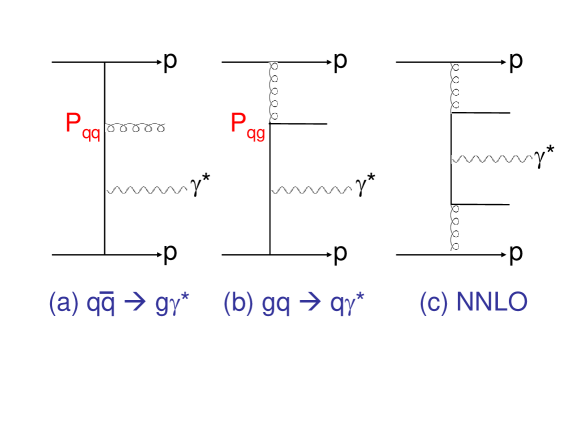
Now let us study the expression for the cross section at NLO. First, we note that the original Feynman integrals corresponding to the NLO matrix element, , do not depend on . However, we will see below how a scale dependence enters. At NLO we may write
| (7) |
where we include the NLO correction to the coefficient function. In terms, for example, of the diagrams (a,b) of Fig. 1 this means that the subprocesses and are now calculated with better, than LLA, accuracy. However part of this contribution was already included, to LLA accuracy, in the second term in (5). So this part should be subtracted from . Moreover, this LLA part depends on the scale . As a result, changing redistributes the order correction between the LO part () and the NLO part (). We see the part of NLO correction which remains after the subtraction, , now depends on the scale , coming from the dependence of the LO LLA term that has been subtracted off. The trick is to choose an appropriate scale, , so to minimize the remaining NLO contribution . To be more precise, we choose a value such that as much as possible of the ‘real’ NLO contribution (which has a ‘ladder-like’ form and which is strongly enhanced by the large value of ) is included in the LO part where all the logarithmically enhanced, , terms are naturally collected by the incoming parton distributions222Actually our approach is rather close to the -factorization method. Using the known NLO result we account for the exact integration in the last cell, adjacent the LO ‘hard’ matrix element (describing heavy photon emission), while the unintegrated parton distribution is generated by the last step of the DGLAP evolution, just like the prescription proposed in [4, 5]..
In the next section we describe how to choose an appropriate scale . Then in Section 3 we demonstrate how by fixing in the LO part of (5), we obtain stability of the Drell-Yan cross section with respect to variations of in the remaining NLO contribution. Moreover, it turns out that the NNLO correction to the Drell-Yan process at such a value of is also very small.
2 The choice of an appropriate factorization scale
DGLAP evolution describes the variation of parton densities with the scale . At LO it accounts for the splitting of a parton to a parton , with the longitudinal momentum fractions which satisfy, and the transverse momenta which satisfy . This splitting is described by Feynman diagrams in the Leading Log Approximation (LLA) where the exact distribution is approximated by the pure logarithmic form .
However the hard matrix element is calculated more precisely. Here we account for the exact dependence. Our aim is to choose the upper limit in the logarithmic integration in such a way that the value of the integral becomes equal to the result given by the NLO matrix element which contains the exact integration. Strictly speaking this cannot be done for all the hard subprocesses simultaneously, with a common value of . So we have to compromise, and to choose for the subprocess which gives the major contribution.
For Drell-Yan production at low , the majority of quarks/antiquarks are produced via the low- gluon to quark splitting, . That is, the most important NLO subprocess is . The corresponding cross section reads
| (8) |
where and . The kinematical upper limit of is
| (9) |
where is the mass of Drell-Yan lepton pair and333Strictly speaking, is the ratio of the light-cone momentum fraction carried by the ‘daughter’ quark to that carried by the ‘parent’ gluon, . .
At first sight, a problem appears to be that, for a large incoming energy, , we will have to consider very large ; that is unreasonably large values of . However, in reality this is not the case. Let us consider the previous splitting, , which produces the gluon from an incoming quark. That is the subprocess. For large energy, , of the incoming system, the gluon flux generated by the fast quark is of the form . Since the cross section (8) decreases as the subenergy increases, weighting the cross section with the gluon flux, results in the main contribution coming from the relatively low region.
An explicit calculation shows that in such a case the pure logarithmic LO evolution integrated up to convoluted with reproduces the NLO contribution of this subprocess. Since in the low- region is the dominant subprocess we anticipate that the choice of will minimize the remaining NLO contribution.
Moreover, at NNLO, for very small , the dominant diagram is , where on both sides of (the Drell-Yan heavy photon) the quark and the antiquark are produced via the gluon to quark splitting, see Fig. 1(c). That is, we have a subprocess with the same kinematics as for the NLO case considered above. It should be also well mimicked by the LO evolution with . Thus the choice will suppress (in a low- domain) the NNLO contribution as well.
3 Scale dependence of low-mass Drell-Yan production
Figs. 2 and 3 show, respectively, the factorization, , and the renormalization, , scale dependences of the cross section as a function of rapidity for the Drell-Yan production444We use the computer code Vrap of Ref. [6]. of a pair of mass GeV at the LHC energy of 7 TeV. As the plots are symmetrical about rapidity , we are able to compare directly two sets of distributions.
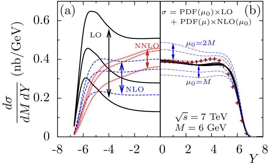
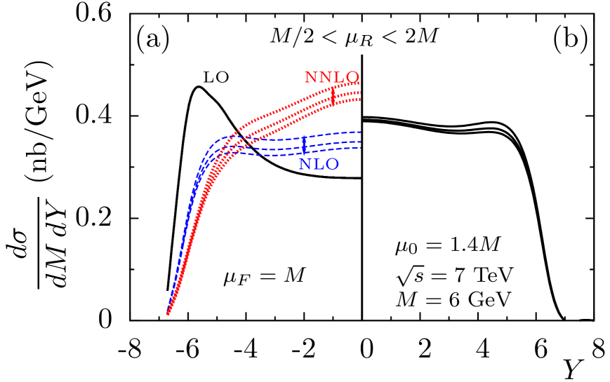
The left-half of each of these plots shows the LO, NLO and NNLO results calculated with the MSTW2008 LO, NLO and the NNLO PDFs [7] respectively. In Fig. 2(a) the renormalization scale is fixed, while the value of factorization scale is varied: . In Fig. 3(a) the factorization scale is fixed , while the renormalization scale is varied: . It is clear that the uncertainties arising from the dependence are huge at the LO, large at the NLO and still not negligible even at the NNLO; see, also, [1]. The dependence on the value of is not so strong, but is still not negligible.
In the right-half of these plots, the continuous bold lines show the cross sections calculated using the PDFs with our ‘optimal’ choice of scale, , in the LO part. The only scale dependence in Fig. 2(b) comes from the variation of in the PDFs convoluted with the remaining NLO contribution. Recall that the value of was found to almost nullify the NLO correction, leaving only a small contribution. Indeed, the plot shows that the distribution has very good stability to the variation of . The dashed lines on this plot (Fig. 2(b)) show that the stability would be much worse if we were to take or , rather than the optimal value of .
Moreover, as we argued in Section 2, even the NNLO correction is rather small for the choice . The corresponding NNLO distribution, calculated with , is shown by the crosses. It is rather close to the (NLO) continuous lines. Recall, here we have used , and the same MSTW2008 NLO PDFs for both the NLO and NNLO calculations, as we wish to see the effect of changing from to leaving the PDFs unchanged. Let us explain why this is the appropriate procedure, since at first sight it may appear that we should use NNLO PDFs for the NNLO prediction.
The basis of our method is that the long evolution length, in (5) with , means that the LLA LO result can capture most of the answer provided that the factorization scale is chosen correctly. That is, the LO term captures most of the NLO contribution for , and even the major part of the NNLO contribution for the same value of .
In general, one may use the known NNLO result to determine another value of the optimal scale, , such that the NLO part (the term in the splitting functions) of DGLAP evolution will capture most of the NNLO contribution. However, as it is seen from Figs. 2 and 3, already the scale used for the LO part (the term in the splitting functions) provides sufficient stability of the results for the Drell-Yan cross section555Recall, that the subtractions of the contribution generated by the NLO DGLAP evolution convoluted with the LO matrix element from the exact NNLO matrix element include the NLO splitting functions. Therefore we can convolute the known NNLO coefficient functions, , with either the NLO or NNLO PDFs, but not with the LO PDF; in the last case we need to recalculate the NNLO matrix element..
In Fig. 3(b) we see an analogous stability with respect to variations of the renormalization scale: , when the factorization scale is fixed at . This additionally confirms that the NLO (and NNLO) corrections are suppressed for the optimal choice of .
4 PDF dependence of low-mass Drell-Yan production
What values of and of the PDFs are probed in Drell-Yan production of a system of mass with rapidity ? Formally, in the collinear approximation, the LO term samples PDFs with precisely known momentum fractions
| (10) |
That is, the distributions are -functions. This is not true in reality. Formula (10) does not include the transverse momenta of the incoming partons. It assumes . If we account for , then we would have
| (11) |
On the other hand, the optimal scale is rather large. For this scale, the partons in the PDFs have ’s up to , which may exceed the value of . In order to get a more realistic impression of the interval of sampled by the process, we go back one step in the DGLAP evolution. That is, we consider the subprocess, which we already discussed at NLO. Recall that actually the majority of low- quarks(antiquarks) were produced just in this way.
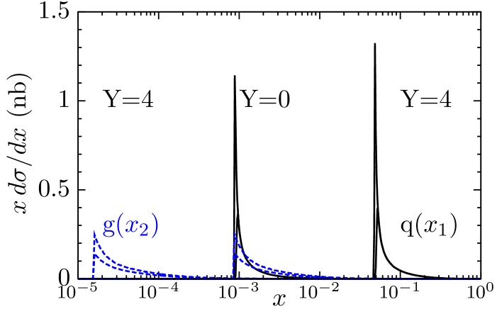
To be specific, let us take the matrix element (8), and convolute it with the NLO MSTW PDFs. Fig. 4 shows the resulting distributions of the momentum fractions of the quark (continuous lines) and the gluon (dashed lines). As before we consider Drell-Yan production of a system of mass GeV at the LHC energy TeV. We show the distributions for two rapidities: and . The very sharp left-hand cutoff of the distributions reflects the fact that the momentum fraction cannot be less than that given by (10). The tail at larger is due to the smearing of the distribution arising from the () subprocess. A narrow peak near the lowest possible value of is due to the singularity in the subprocess cross section (8).
To calculate the distributions shown in Fig. 4 we introduced the infrared cutoff , with GeV (the smallest virtuality at which the DGLAP evolution starts). For a larger cutoff666In the case of we come back to -functions at the values given by (10)., GeV we get the lower peaks shown in the diagram. For the cutoff GeV, the subprocess gives more than 90% of the whole Drell-Yan cross section. Thus the distributions shown in Fig. 4 provide a rather good evaluation of the -regions sampled by the Drell-Yan process for these kinematics.
What information about PDFs do we obtain from measurements of low-mass Drell-Yan lepton-pairs at high rapidity? It is important to emphasize that the data make a direct measurement of the quark/antiquark PDFs at the optimal scale , with little factorization or renormalization scale ambiguity, for the values of given by (10). That is, there is a direct one-to-one correspondence between the data and the PDFs. For example, the production of a low-mass GeV pair at 7 TeV, going forward with rapidity , measures quark/antiquark PDFs with
| (12) |
but at a moderately high scale, .
What is the impact of such measurements on global PDF analyses? Clearly, the measurements can probe a small domain so far unexplored by data. If, at such small , we were to believe in pure DGLAP evolution, then the majority of the low quarks (antiquarks) comes from the splitting. Therefore the dependence of the Drell-Yan cross section will probe the gluon distribution in a similar way to how the scaling violations in deep inelastic scattering data, , probe, via DGLAP evolution, the low gluon density777Recall, that starting the evolution from GeV more than 90% of the Drell-Yan cross section is described by the subprocess, and so will probe , see Fig. 4.. So, by including low-mass high-rapidity Drell-Yan data in the global parton analysis we will strongly constrain the low gluon PDF. Note that Drell-Yan data at the LHC may probe very low values of . In this future global analysis we should account for the absorptive, ln, etc., modifications to the evolution equations, as well as using the Drell-Yan data at the optimal scale.
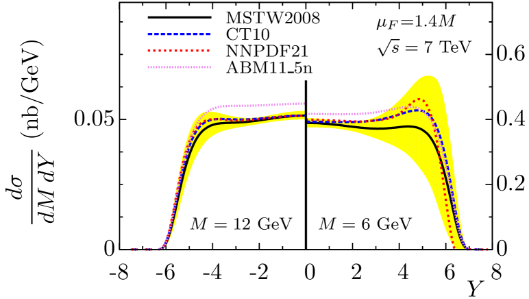
Bearing in mind the above qualifications, let us use recent sets of existing global PDFs to calculate the cross section for the examples of and GeV lepton-pair production. The results are shown in Fig. 5. The scales in the figure have been adjusted to allow for the naive behaviour of the cross section, so that any departure from the ‘symmetry’ of the plot is due to the PDFs.
At first sight, it might be surprising that there is not more difference between the predictions from the different sets of PDFs for such low values of . However,
-
(a)
the predictions made by using all reasonable sets of PDFs which are consistent with each other within the error bands;
-
(b)
the partons are being probed at a moderately high scale: and 280 GeV2 where the difference between different sets of PDFs is not large;
-
(c)
recall that, at the moment, there is no prediction for , but only those based on ‘ad hoc’ PDF extrapolations to very low ; however, the forthcoming LHCb data can provide an important direct measurement of the PDFs in this low- region; a domain which is not accessible by previous data.
5 Conclusion
The observation of low-mass Drell-Yan pairs at high rapidity at the LHC can probe the PDFs in a low domain unreachable in previous experiments; that is, . However, the constraints on the PDFs found using a conventional analysis of the data, show great sensitivity to the choice of factorization (and renormalization) scale. Here we have introduced a technique to determine an optimal scale which greatly reduces this sensitivity. The optimal scale is found to be , where is the mass of the produced pair. Simply for illustration, we show ‘predictions’ of the Drell-Yan cross section, as a function of rapidity, , for and GeV for a variety of recent PDF sets, but we stress that the predictions for depend on ‘ad hoc’ extrapolations. Here, LHC data can, for the first time, make a direct measurement of PDFs in the domain.
Acknowledgements
We thank Ronan McNulty for useful discussions. EGdO and MGR thank the IPPP at the University of Durham for hospitality. This work was supported by the grant RFBR 11-02-00120-a and by the Federal Program of the Russian State RSGSS-65751.2010.2; and by FAPESP (Brazil) under contract 2011/50597-8.
References
- [1] A.D. Martin, W.J. Stirling, R.S. Thorne and G. Watt, Proc. of DIS2008, London, 30; arXiv:0808.1847.
- [2] E.G. de Oliveira, A.D. Martin and M.G. Ryskin, Eur. Phys. J. C71, 1727 (2011)
- [3] LHCb Collaboration, private communication; Phys. Lett. B694, 209 (2010).
- [4] M.A. Kimber, A.D. Martin and M.G. Ryskin, Phys. Rev. D63, 114027 (2001).
- [5] A.D. Martin, M.G. Ryskin and G. Watt, Eur. Phys. J. C66, 163 (2010).
- [6] C. Anastasiou, L.J. Dixon, K. Melnikov and F. Petriello, Phys. Rev. D69, 094008 (2004).
- [7] A.D. Martin, W.J. Stirling, R.S. Thorne and G. Watt, Eur. Phys. J. C63, 189 (2009).
- [8] H.-L. Lai et al., Phys. Rev. D82, 074024 (2010).
- [9] NNPDF Collaboration, R.D. Ball et al., Nucl. Phys. B849, 296 (2011); Nucl. Phys. B855 153 (2012).
- [10] S. Alekhin, J. Blümlein and S. Moch, arXiv:1202.2281