Ghost Force Influence of a Quasicontinuum Method in Two Dimension

Jingrun Chen Institute of Computational Mathematics and Scientific/Engineering Computing, AMSS, Chinese Academy of Sciences, No. 55, Zhong-Guan-Cun East Road, Beijing, 100190, China chenjr@lsec.cc.ac.cn South Hall 6705, Mathematics Department, University of California, Santa Barbara, CA93106, USA cjr@math.ucsb.edu ย andย  Pingbing Ming LSEC, Institute of Computational Mathematics and Scientific/Engineering Computing, AMSS, Chinese Academy of Sciences, No. 55 Zhong-Guan-Cun East Road, Beijing, 100190, China mpb@lsec.cc.ac.cn
Abstract.

We derive an analytical expression for the solution of a two-dimensional quasicontinuum method with a planar interface. The expression is used to prove that the ghost force may lead to a finite size error for the gradient of the solution. We estimate the width of the interfacial layer induced by the ghost force is of ๐’ชโ€‹(ฮต)๐’ช๐œ€\mathcal{O}(\sqrt{\varepsilon}\,) with ฮต๐œ€\varepsilon the equilibrium bond length, which is much wider than that of the one-dimensional problem.

Key words and phrases:
Quasicontinuum method, ghost force, interfacial layer
2000 Mathematics Subject Classification:
65N30, 65N12, 65N06, 74G20, 74G15
The work of Ming was partially supported by National Natural Science Foundation of China grants 10932011, by the funds from Creative Research Groups of China through grant 11021101, and by the support of CAS National Center for Mathematics and Interdisciplinary Sciences. The authors are grateful to Weinan E and Jianfeng Lu for helpful discussions.

1. Introduction

Multiscale methods have been developed to simulate mechanical behaviors of solids for several decadesย [14]. Combination of models at different scales greatly enhances the dimension of problems that computers can deal with. However, problems regarding the consistency, stability and convergence of the multiscale methods may arise from the couplingย [3]. Taking the quasicontinuum (QC) methodย [17, 10] for example, one of the main issues is the so called ghost force problemย [16], which is the artificial non-zero force that the atoms experience at the equilibrium state. In the language of numerical analysis, the scheme lacks consistency at the interface between the atomistic region and the continuum regionย [4]. For the one-dimensional problem, it has been shown inย [15] that the ghost force may lead to a finite size error for the gradient of the solution. This generates an interfacial layer with width ๐’ชโ€‹(ฮตโ€‹|lnโกฮต|)๐’ช๐œ€๐œ€\mathcal{O}(\varepsilon\lvert\ln\varepsilon\rvert), out of which the error for the gradient of the solution is of ๐’ชโ€‹(ฮต)๐’ช๐œ€\mathcal{O}(\varepsilon).

To understand the influence of the ghost force for high dimensional problems, we study a two-dimensional triangular lattice model with a QC approximation. This QC method couples the Cauchy-Born elasticity model and the atomistic model with a planar interface. Numerical results show that the ghost force may lead to a finite size error for the gradient of the solution as in the one-dimensional problem. The error profile exhibits a layer-like structure. It seems that the width of the interfacial layer induced by the ghost force is of ๐’ชโ€‹(ฮต)๐’ช๐œ€\mathcal{O}(\sqrt{\varepsilon}), which is much wider than that of the one-dimensional problem.

To further characterize the influence of the ghost force, we introduce a square lattice model with a QC approximation. Compared to the triangular lattice model, this model can be solved analytically and the error profile exhibits a clear layer-like structure. Based on the analytical solution, we prove the error committed by the ghost force for the gradient of the solution is ๐’ชโ€‹(1)๐’ช1\mathcal{O}(1) and the width of the induced interfacial layer is of ๐’ชโ€‹(ฮต)๐’ช๐œ€\mathcal{O}(\sqrt{\varepsilon}), which are also confirmed by the numerical results.

The paper is organized as follows. Numerical results for the triangular model and the square lattice model with QC approximations are presented inย ยงย 2 andย ยงย 3, respectively. We derive an analytical expression of the solution of the square lattice model with a QC approximation inย ยงย 4. The main results of the paper are proved inย ยงย 5.

2. A quasicontinuum method for triangular lattice

2.1. Atomistic and continuum models

We consider the triangular lattice ๐•ƒ๐•ƒ\mathbb{L}, which can be written as

๐•ƒ={xโˆˆโ„2โˆฃx=mโ€‹a1+nโ€‹a2,m,nโˆˆโ„ค}๐•ƒconditional-set๐‘ฅsuperscriptโ„2formulae-sequence๐‘ฅ๐‘šsubscript๐‘Ž1๐‘›subscript๐‘Ž2๐‘š๐‘›โ„ค\mathbb{L}=\{\,x\in\mathbb{R}^{2}\,\mid\,x=ma_{1}+na_{2},\;m,n\in\mathbb{Z}\,\}

with the basis vectors a1=(1,0),a2=(1/2,3/2)formulae-sequencesubscript๐‘Ž110subscript๐‘Ž21232a_{1}=(1,0),a_{2}=(1/2,\sqrt{3}/2). Define the unit cell of ๐•ƒ๐•ƒ\mathbb{L} as

ฮ“={xโˆˆโ„2โˆฃx=c1โ€‹a1+c2โ€‹a2,โˆ’1/2โ‰คc1,c2<1/2}.ฮ“conditional-set๐‘ฅsuperscriptโ„2formulae-sequence๐‘ฅsubscript๐‘1subscript๐‘Ž1subscript๐‘2subscript๐‘Ž2formulae-sequence12subscript๐‘1subscript๐‘212\Gamma=\{\,x\in\mathbb{R}^{2}\,\mid\,x=c_{1}a_{1}+c_{2}a_{2},\;-1/2\leq c_{1},c_{2}<1/2\,\}.

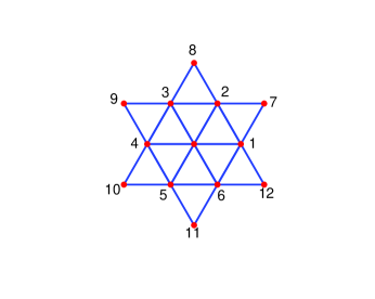
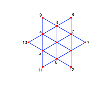
We shall consider lattice system ฮตโ€‹๐•ƒ๐œ€๐•ƒ\varepsilon\mathbb{L} inside the domain ฮฉฮฉ\Omega, and ฮฉฮต=ฮฉโˆฉฮตโ€‹๐•ƒsubscriptฮฉ๐œ€ฮฉ๐œ€๐•ƒ\Omega_{\varepsilon}=\Omega\cap\varepsilon\mathbb{L}, where ฮต๐œ€\varepsilon is the equilibrium bond length. Assume that the atoms are interacted with the potential function V๐‘‰V, which is usually a highly nonlinear function, e.g., the Lennard-Jones potentialย [12]. Denote by ๐’ฎ1subscript๐’ฎ1\mathcal{S}_{1} and ๐’ฎ2subscript๐’ฎ2\mathcal{S}_{2} the first and the second neighborhood interaction ranges; see Figureย 1. In particular, we have

๐’ฎ1subscript๐’ฎ1\displaystyle\mathcal{S}_{1} =โˆชi=16si={a1,a2,โˆ’a1+a2,โˆ’a1,โˆ’a2,a1โˆ’a2},absentsuperscriptsubscript๐‘–16subscript๐‘ ๐‘–subscript๐‘Ž1subscript๐‘Ž2subscript๐‘Ž1subscript๐‘Ž2subscript๐‘Ž1subscript๐‘Ž2subscript๐‘Ž1subscript๐‘Ž2\displaystyle=\cup_{i=1}^{6}s_{i}=\{a_{1},a_{2},-a_{1}+a_{2},-a_{1},-a_{2},a_{1}-a_{2}\},
๐’ฎ2subscript๐’ฎ2\displaystyle\mathcal{S}_{2} =โˆชi=712si={a1+a2,โˆ’a1+2โ€‹a2,โˆ’2โ€‹a1+a2,โˆ’a1โˆ’a2,a1โˆ’2โ€‹a2,2โ€‹a1โˆ’a2}.absentsuperscriptsubscript๐‘–712subscript๐‘ ๐‘–subscript๐‘Ž1subscript๐‘Ž2subscript๐‘Ž12subscript๐‘Ž22subscript๐‘Ž1subscript๐‘Ž2subscript๐‘Ž1subscript๐‘Ž2subscript๐‘Ž12subscript๐‘Ž22subscript๐‘Ž1subscript๐‘Ž2\displaystyle=\cup_{i=7}^{12}s_{i}=\{a_{1}+a_{2},-a_{1}+2a_{2},-2a_{1}+a_{2},-a_{1}-a_{2},a_{1}-2a_{2},2a_{1}-a_{2}\}.

For ฮผโˆˆโ„ค2๐œ‡superscriptโ„ค2\mu\in\mathbb{Z}^{2}, the translation operator Tฮตฮผsubscriptsuperscript๐‘‡๐œ‡๐œ€T^{\mu}_{\varepsilon} is defined for any lattice function z:๐•ƒโ†’โ„2:๐‘งโ†’๐•ƒsuperscriptโ„2z:\mathbb{L}\to\mathbb{R}^{2} as

(Tฮตฮผโ€‹z)โ€‹(x)=zโ€‹(x+ฮตโ€‹ฮผ1โ€‹a1+ฮตโ€‹ฮผ2โ€‹a2)forย โ€‹xโˆˆ๐•ƒ.formulae-sequencesubscriptsuperscript๐‘‡๐œ‡๐œ€๐‘ง๐‘ฅ๐‘ง๐‘ฅ๐œ€subscript๐œ‡1subscript๐‘Ž1๐œ€subscript๐œ‡2subscript๐‘Ž2forย ๐‘ฅ๐•ƒ(T^{\mu}_{\varepsilon}z)(x)=z(x+\varepsilon\mu_{1}a_{1}+\varepsilon\mu_{2}a_{2})\quad\text{for }x\in\mathbb{L}.

We define the forward and backward discrete gradient operators as

Ds+=ฮตโˆ’1โ€‹(Tฮตฮผโˆ’I)andDsโˆ’=ฮตโˆ’1โ€‹(Iโˆ’Tฮตฮผ),formulae-sequencesuperscriptsubscript๐ท๐‘ superscript๐œ€1subscriptsuperscript๐‘‡๐œ‡๐œ€๐ผandsuperscriptsubscript๐ท๐‘ superscript๐œ€1๐ผsubscriptsuperscript๐‘‡๐œ‡๐œ€D_{s}^{+}=\varepsilon^{-1}(T^{\mu}_{\varepsilon}-I)\qquad\text{and}\qquad D_{s}^{-}=\varepsilon^{-1}(I-T^{\mu}_{\varepsilon}),

where s=ฮผ1โ€‹a1+ฮผ2โ€‹a2๐‘ subscript๐œ‡1subscript๐‘Ž1subscript๐œ‡2subscript๐‘Ž2s=\mu_{1}a_{1}+\mu_{2}a_{2} and I๐ผI is the identity operator. We shall also use the short-hand Dโ€‹z=(D1+โ€‹z,D2+โ€‹z)=(Ds1+โ€‹z,Ds2+โ€‹z)๐ท๐‘งsuperscriptsubscript๐ท1๐‘งsuperscriptsubscript๐ท2๐‘งsuperscriptsubscript๐ทsubscript๐‘ 1๐‘งsuperscriptsubscript๐ทsubscript๐‘ 2๐‘งDz=(D_{1}^{+}z,D_{2}^{+}z)=(D_{s_{1}}^{+}z,D_{s_{2}}^{+}z).

Refer to caption
Figure 1. The first and second neighborhood interaction ranges of the triangular lattice; ๐’ฎ1={s1,โ‹ฏ,s6}subscript๐’ฎ1subscript๐‘ 1โ‹ฏsubscript๐‘ 6\mathcal{S}_{1}=\{s_{1},\cdots,s_{6}\} and ๐’ฎ2={s7,โ‹ฏ,s12}subscript๐’ฎ2subscript๐‘ 7โ‹ฏsubscript๐‘ 12\mathcal{S}_{2}=\{s_{7},\cdots,s_{12}\}.

Consider an atomic system posed on ฮฉฮตsubscriptฮฉ๐œ€\Omega_{\varepsilon}. The total energy is given by

(2.1) Eattot=12โ€‹โˆ‘xโˆˆฮฉฮตโˆ‘sโˆˆ๐’ฎ1โˆช๐’ฎ2Vโ€‹(|Ds+โ€‹zโ€‹(x)|),subscriptsuperscript๐ธtotat12subscript๐‘ฅsubscriptฮฉ๐œ€subscript๐‘ subscript๐’ฎ1subscript๐’ฎ2๐‘‰superscriptsubscript๐ท๐‘ ๐‘ง๐‘ฅE^{\text{tot}}_{\text{at}}=\dfrac{1}{2}\sum_{x\in\Omega_{\varepsilon}}\sum_{s\in\mathcal{S}_{1}\cup\mathcal{S}_{2}}V\left(\lvert D_{s}^{+}z(x)\rvert\right),

where V๐‘‰V is a potential function. In this paper, we only consider the pairwise potential function, and leave the discussion on the more general potential functions in future publication. The atomistic problem is to minimize the total energy subject to certain boundary conditions that will be specified later on.

Next we turn to the Cauchy-Born elasticity modelย [1, 6, 5, 7]. Given a 222 by 222 matrix A๐ดA, the stored energy density function is given by

Wcbโ€‹(A)=12โ€‹ฯ‘0โ€‹โˆ‘sโˆˆ๐’ฎ1โˆช๐’ฎ2Vโ€‹(|sโ‹…A|),subscript๐‘Šcb๐ด12subscriptitalic-ฯ‘0subscript๐‘ subscript๐’ฎ1subscript๐’ฎ2๐‘‰โ‹…๐‘ ๐ดW_{\text{cb}}(A)=\dfrac{1}{2\vartheta_{0}}\sum_{s\in\mathcal{S}_{1}\cup\mathcal{S}_{2}}V(\lvert s\cdot A\rvert),

where ฯ‘0subscriptitalic-ฯ‘0\vartheta_{0} is the area of the unit cell and ฯ‘0=3โ€‹ฮต2/2subscriptitalic-ฯ‘03superscript๐œ€22\vartheta_{0}=\sqrt{3}\varepsilon^{2}/2. The stored energy function is defined by

Ecbtot=โˆซฮฉWcbโ€‹(โˆ‡zโ€‹(x))โ€‹dx.subscriptsuperscript๐ธtotcbsubscriptฮฉsubscript๐‘Šcbโˆ‡๐‘ง๐‘ฅdifferential-d๐‘ฅE^{\text{tot}}_{\text{cb}}=\int_{\Omega}W_{\text{cb}}(\nabla z(x))\,\mathrm{d}\,x.

The continuum problem is to minimize the stored energy function subject to certain boundary conditions. We employ the standard P1subscript๐‘ƒ1P_{1} Lagrange finite element to approximate the Cauchy-Born elasticity model with the lattice ๐•ƒ๐•ƒ\mathbb{L} as the triangulation. The approximate stored energy function is

(2.2) Ecb,ฮตtot=12โ€‹โˆ‘xโˆˆฮฉฮตโˆ‘i=16(Vโ€‹(|Dsi+โ€‹zโ€‹(x)|)+Vโ€‹(|(Dsi++Dsi+1+)โ€‹zโ€‹(x)|)).subscriptsuperscript๐ธtotcb๐œ€12subscript๐‘ฅsubscriptฮฉ๐œ€superscriptsubscript๐‘–16๐‘‰superscriptsubscript๐ทsubscript๐‘ ๐‘–๐‘ง๐‘ฅ๐‘‰superscriptsubscript๐ทsubscript๐‘ ๐‘–superscriptsubscript๐ทsubscript๐‘ ๐‘–1๐‘ง๐‘ฅE^{\text{tot}}_{\text{cb},\varepsilon}=\dfrac{1}{2}\sum_{x\in\Omega_{\varepsilon}}\sum_{i=1}^{6}\left(V\left(\lvert D_{s_{i}}^{+}z(x)\rvert\right)+V\left(\lvert(D_{s_{i}}^{+}+D_{s_{i+1}}^{+})z(x)\rvert\right)\right).

One can see Ecb,ฮตtotsubscriptsuperscript๐ธtotcb๐œ€E^{\text{tot}}_{\text{cb},\varepsilon} reproduces the atomistic energy Eattotsubscriptsuperscript๐ธtotatE^{\text{tot}}_{\text{at}}; cf.ย (2.1), if only the nearest neighborhood interaction is considered.

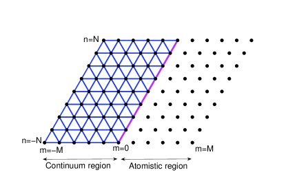
We study the quasicontinuum methodย [17]. Let ฮต=1/(2โ€‹M)๐œ€12๐‘€\varepsilon=1/(2M). We assume that the interface between the continuum model and the atomistic model is x1=0subscript๐‘ฅ10x_{1}=0 as shown in Figureย 2. The total energy of the QC method is

Eqctotsubscriptsuperscript๐ธtotqc\displaystyle E^{\text{tot}}_{\text{qc}} =12โ€‹โˆ‘x1โ‰คโˆ’2โ€‹ฮตโˆ‘i=16(Vโ€‹(|Dsi+โ€‹zโ€‹(x)|)+Vโ€‹(|(Dsi++Dsi+1+)โ€‹zโ€‹(x)|))absent12subscriptsubscript๐‘ฅ12๐œ€superscriptsubscript๐‘–16๐‘‰superscriptsubscript๐ทsubscript๐‘ ๐‘–๐‘ง๐‘ฅ๐‘‰superscriptsubscript๐ทsubscript๐‘ ๐‘–superscriptsubscript๐ทsubscript๐‘ ๐‘–1๐‘ง๐‘ฅ\displaystyle=\dfrac{1}{2}\sum_{x_{1}\leq-2\varepsilon}\sum_{i=1}^{6}\left(V\left(\lvert D_{s_{i}}^{+}z(x)\rvert\right)+V\left(\lvert(D_{s_{i}}^{+}+D_{s_{i+1}}^{+})z(x)\rvert\right)\right)
+12โ€‹โˆ‘x1=โˆ’ฮต{โˆ‘i=16(Vโ€‹(|Dsi+โ€‹zโ€‹(x)|)+Vโ€‹(|(Dsi++Dsi+1+)โ€‹zโ€‹(x)|))+Vโ€‹(|Ds12+โ€‹zโ€‹(x)|)}12subscriptsubscript๐‘ฅ1๐œ€superscriptsubscript๐‘–16๐‘‰superscriptsubscript๐ทsubscript๐‘ ๐‘–๐‘ง๐‘ฅ๐‘‰superscriptsubscript๐ทsubscript๐‘ ๐‘–superscriptsubscript๐ทsubscript๐‘ ๐‘–1๐‘ง๐‘ฅ๐‘‰superscriptsubscript๐ทsubscript๐‘ 12๐‘ง๐‘ฅ\displaystyle\quad+\dfrac{1}{2}\sum_{x_{1}=-\varepsilon}\bigg{\{}\sum_{i=1}^{6}\left(V\left(\lvert D_{s_{i}}^{+}z(x)\rvert\right)+V\left(\lvert(D_{s_{i}}^{+}+D_{s_{i+1}}^{+})z(x)\rvert\right)\right)+V(\lvert D_{s_{12}}^{+}z(x)\rvert)\bigg{\}}
+12โˆ‘x1=0{โˆ‘sโˆˆ๐’ฎ1V(|Ds+z(x)|)+โˆ‘i=24(V(|Dsi+z(x)|)+V(|(Dsi++Dsi+1+)z(x)|))\displaystyle\quad+\dfrac{1}{2}\sum_{x_{1}=0}\bigg{\{}\sum_{s\in\mathcal{S}_{1}}V\left(\lvert D_{s}^{+}z(x)\rvert\right)+\sum_{i=2}^{4}\left(V\left(\lvert D_{s_{i}}^{+}z(x)\rvert\right)+V\left(\lvert(D_{s_{i}}^{+}+D_{s_{i+1}}^{+})z(x)\rvert\right)\right)
+12V(|Ds7+z(x)|)+V(|Ds11+z(x)|)+V(|Ds12+z(x)|)}\displaystyle\phantom{+\dfrac{1}{2}\sum_{x_{1}=0}\bigg{\{}}\qquad+\dfrac{1}{2}V(\lvert D_{s_{7}}^{+}z(x)\rvert)+V(\lvert D_{s_{11}}^{+}z(x)\rvert)+V(\lvert D_{s_{12}}^{+}z(x)\rvert)\bigg{\}}
+12โ€‹โˆ‘x1=ฮต{โˆ‘sโˆˆ๐’ฎ1โˆช๐’ฎ2Vโ€‹(|Ds+โ€‹zโ€‹(x)|)โˆ’12โ€‹Vโ€‹(|Ds9+โ€‹zโ€‹(x)|)}12subscriptsubscript๐‘ฅ1๐œ€subscript๐‘ subscript๐’ฎ1subscript๐’ฎ2๐‘‰superscriptsubscript๐ท๐‘ ๐‘ง๐‘ฅ12๐‘‰superscriptsubscript๐ทsubscript๐‘ 9๐‘ง๐‘ฅ\displaystyle\quad+\dfrac{1}{2}\sum_{x_{1}=\varepsilon}\bigg{\{}\sum_{s\in\mathcal{S}_{1}\cup\mathcal{S}_{2}}V\left(\lvert D_{s}^{+}z(x)\rvert\right)-\dfrac{1}{2}V(\lvert D_{s_{9}}^{+}z(x)\rvert)\bigg{\}}
+12โ€‹โˆ‘x1โ‰ฅ2โ€‹ฮตโˆ‘sโˆˆ๐’ฎ1โˆช๐’ฎ2Vโ€‹(|Ds+โ€‹zโ€‹(x)|).12subscriptsubscript๐‘ฅ12๐œ€subscript๐‘ subscript๐’ฎ1subscript๐’ฎ2๐‘‰superscriptsubscript๐ท๐‘ ๐‘ง๐‘ฅ\displaystyle\quad+\dfrac{1}{2}\sum_{x_{1}\geq 2\varepsilon}\sum_{s\in\mathcal{S}_{1}\cup\mathcal{S}_{2}}V\left(\lvert D_{s}^{+}z(x)\rvert\right).

The force at atom x๐‘ฅx is defined by

โ„ฑqcโ€‹[z]โ€‹(x)โ‰กโˆ’โˆ‚Eqctotโˆ‚zโ€‹(x).subscriptโ„ฑqcdelimited-[]๐‘ง๐‘ฅsubscriptsuperscript๐ธtotqc๐‘ง๐‘ฅ\mathcal{F}_{\text{qc}}[z](x)\equiv-\dfrac{\partial E^{\text{tot}}_{\text{qc}}}{\partial z(x)}.

Since we only concern the influence of the ghost force, followingย [15], we assume that the potential function is a harmonic function, i.e.,

Vโ€‹(r)=12โ€‹r2.๐‘‰๐‘Ÿ12superscript๐‘Ÿ2V(r)=\dfrac{1}{2}{r^{2}}.

Without taking into account the external force, we write the equilibrium equations for the QC approximation as

โ„ฑqcโ€‹[z]โ€‹(x)=0subscriptโ„ฑqcdelimited-[]๐‘ง๐‘ฅ0\mathcal{F}_{\text{qc}}[z](x)=0

with

โ„ฑqcโ€‹[z]โ€‹(x)subscriptโ„ฑqcdelimited-[]๐‘ง๐‘ฅ\displaystyle\mathcal{F}_{\text{qc}}[z](x) =โˆ’12โ€‹zโ€‹(x)+โˆ‘i=112zโ€‹(x+ฮตโ€‹si),absent12๐‘ง๐‘ฅsuperscriptsubscript๐‘–112๐‘ง๐‘ฅ๐œ€subscript๐‘ ๐‘–\displaystyle=-12z(x)+\sum_{i=1}^{12}z(x+\varepsilon s_{i}), xโˆˆฮฉฮต,x1โ‰คโˆ’2โ€‹ฮต,formulae-sequence๐‘ฅsubscriptฮฉ๐œ€subscript๐‘ฅ12๐œ€\displaystyle x\in\Omega_{\varepsilon},x_{1}\leq-2\varepsilon,
โ„ฑqcโ€‹[z]โ€‹(x)subscriptโ„ฑqcdelimited-[]๐‘ง๐‘ฅ\displaystyle\mathcal{F}_{\text{qc}}[z](x) =โˆ’24โ€‹zโ€‹(x)+4โ€‹โˆ‘i=16zโ€‹(x+ฮตโ€‹si),absent24๐‘ง๐‘ฅ4superscriptsubscript๐‘–16๐‘ง๐‘ฅ๐œ€subscript๐‘ ๐‘–\displaystyle=-24z(x)+4\sum_{i=1}^{6}z(x+\varepsilon s_{i}), xโˆˆฮฉฮต,x1โ‰ฅ2โ€‹ฮต.formulae-sequence๐‘ฅsubscriptฮฉ๐œ€subscript๐‘ฅ12๐œ€\displaystyle x\in\Omega_{\varepsilon},x_{1}\geq 2\varepsilon.
Refer to caption
Figure 2. Schematic picture of ฮฉฮตsubscriptฮฉ๐œ€\Omega_{\varepsilon}.

For x=(โˆ’ฮต,x2)๐‘ฅ๐œ€subscript๐‘ฅ2x=(-\varepsilon,x_{2}),

โ„ฑqcโ€‹[z]โ€‹(x)=โˆ’492โ€‹zโ€‹(x)+4โ€‹โˆ‘i=16zโ€‹(x+ฮตโ€‹si)+12โ€‹zโ€‹(x+ฮตโ€‹s12).subscriptโ„ฑqcdelimited-[]๐‘ง๐‘ฅ492๐‘ง๐‘ฅ4superscriptsubscript๐‘–16๐‘ง๐‘ฅ๐œ€subscript๐‘ ๐‘–12๐‘ง๐‘ฅ๐œ€subscript๐‘ 12\mathcal{F}_{\text{qc}}[z](x)=-\dfrac{49}{2}z(x)+4\sum_{i=1}^{6}z(x+\varepsilon s_{i})+\dfrac{1}{2}z(x+\varepsilon s_{12}).

For x=(0,x2)๐‘ฅ0subscript๐‘ฅ2x=(0,x_{2}),

โ„ฑqcโ€‹[z]โ€‹(x)subscriptโ„ฑqcdelimited-[]๐‘ง๐‘ฅ\displaystyle\mathcal{F}_{\text{qc}}[z](x) =โˆ’18โ€‹zโ€‹(x)+[zโ€‹(x+ฮตโ€‹s1)+zโ€‹(x+ฮตโ€‹s6)]+52โ€‹[zโ€‹(x+ฮตโ€‹s2)+zโ€‹(x+ฮตโ€‹s5)]absent18๐‘ง๐‘ฅdelimited-[]๐‘ง๐‘ฅ๐œ€subscript๐‘ 1๐‘ง๐‘ฅ๐œ€subscript๐‘ 652delimited-[]๐‘ง๐‘ฅ๐œ€subscript๐‘ 2๐‘ง๐‘ฅ๐œ€subscript๐‘ 5\displaystyle=-18z(x)+[z(x+\varepsilon s_{1})+z(x+\varepsilon s_{6})]+\dfrac{5}{2}[z(x+\varepsilon s_{2})+z(x+\varepsilon s_{5})]
+4โ€‹[zโ€‹(x+ฮตโ€‹s3)+zโ€‹(x+ฮตโ€‹s4)]+[zโ€‹(x+ฮตโ€‹s7)+zโ€‹(x+ฮตโ€‹s11)+zโ€‹(x+ฮตโ€‹s12)].4delimited-[]๐‘ง๐‘ฅ๐œ€subscript๐‘ 3๐‘ง๐‘ฅ๐œ€subscript๐‘ 4delimited-[]๐‘ง๐‘ฅ๐œ€subscript๐‘ 7๐‘ง๐‘ฅ๐œ€subscript๐‘ 11๐‘ง๐‘ฅ๐œ€subscript๐‘ 12\displaystyle\quad+4[z(x+\varepsilon s_{3})+z(x+\varepsilon s_{4})]+[z(x+\varepsilon s_{7})+z(x+\varepsilon s_{11})+z(x+\varepsilon s_{12})].

For x=(ฮต,x2)๐‘ฅ๐œ€subscript๐‘ฅ2x=(\varepsilon,x_{2}),

โ„ฑqcโ€‹[z]โ€‹(x)=โˆ’232โ€‹zโ€‹(x)+โˆ‘i=112zโ€‹(x+ฮตโ€‹si)โˆ’12โ€‹zโ€‹(x+ฮตโ€‹s9).subscriptโ„ฑqcdelimited-[]๐‘ง๐‘ฅ232๐‘ง๐‘ฅsuperscriptsubscript๐‘–112๐‘ง๐‘ฅ๐œ€subscript๐‘ ๐‘–12๐‘ง๐‘ฅ๐œ€subscript๐‘ 9\mathcal{F}_{\text{qc}}[z](x)=-\dfrac{23}{2}z(x)+\sum_{i=1}^{12}z(x+\varepsilon s_{i})-\dfrac{1}{2}z(x+\varepsilon s_{9}).

At the equilibrium state, we evaluate โ„ฑqcsubscriptโ„ฑqc\mathcal{F}_{\text{qc}} at zโ€‹(x)=x๐‘ง๐‘ฅ๐‘ฅz(x)=x to get

โ„ฑqc[x](x)={(โˆ’3โ€‹ฮต/4,3โ€‹ฮต/4),ifx1=โˆ’ฮต,(3โ€‹ฮต/2,โˆ’3โ€‹ฮต/2),ifx1=0,(โˆ’3โ€‹ฮต/4,3โ€‹ฮต/4),ifx1=ฮต,(0,0),otherwise.\mathcal{F}_{\text{qc}}[x](x)=\left\{\begin{aligned} (-3\varepsilon/4,\sqrt{3}\varepsilon/4),&\rm{\quad if\quad}x_{1}=-\varepsilon,\\ (3\varepsilon/2,-\sqrt{3}\varepsilon/2),&\rm{\quad if\quad}x_{1}=0,\\ (-3\varepsilon/4,\sqrt{3}\varepsilon/4),&\rm{\quad if\quad}x_{1}=\varepsilon,\\ (0,0),&\rm{\quad otherwise}.\end{aligned}\right.

The above equations imply z1โ€‹(x)=โˆ’3โ€‹z2โ€‹(x)subscript๐‘ง1๐‘ฅ3subscript๐‘ง2๐‘ฅz_{1}(x)=-\sqrt{3}z_{2}(x). Therefore, we only study the first component of zโ€‹(x)๐‘ง๐‘ฅz(x) and neglect the subscript if no confusion will occur. The error of the displacement induced by the ghost force, denoted by yโ€‹(x)โ‰กzโ€‹(x)โˆ’x๐‘ฆ๐‘ฅ๐‘ง๐‘ฅ๐‘ฅy(x)\equiv z(x)-x, satisfies

(2.3) โ„ฑqcโ€‹[y]โ€‹(x)=โ„ฑqcโ€‹[z]โ€‹(x)โˆ’โ„ฑqcโ€‹[x]โ€‹(x)=โˆ’โ„ฑqcโ€‹[x]โ€‹(x)โ‰กfโ€‹(x)subscriptโ„ฑqcdelimited-[]๐‘ฆ๐‘ฅsubscriptโ„ฑqcdelimited-[]๐‘ง๐‘ฅsubscriptโ„ฑqcdelimited-[]๐‘ฅ๐‘ฅsubscriptโ„ฑqcdelimited-[]๐‘ฅ๐‘ฅ๐‘“๐‘ฅ\mathcal{F}_{\text{qc}}[y](x)=\mathcal{F}_{\text{qc}}[z](x)-\mathcal{F}_{\text{qc}}[x](x)=-\mathcal{F}_{\text{qc}}[x](x)\equiv f(x)

with

f(x)={3โ€‹ฮต/4,ย ifย โ€‹x1=โˆ’ฮต,โˆ’3โ€‹ฮต/2,ifx1=0,3โ€‹ฮต/4,ifx1=ฮต,0otherwise.f(x)=\left\{\begin{aligned} 3\varepsilon/4,&\text{\quad if\quad}x_{1}=-\varepsilon,\\ -3\varepsilon/2,&\rm{\quad if\quad}x_{1}=0,\\ 3\varepsilon/4,&\rm{\quad if\quad}x_{1}=\varepsilon,\\ 0&\rm{\quad otherwise}.\end{aligned}\right.

Boundary conditions need to be supplemented to close the system of equilibrium equations. Two types of boundary conditions will be considered in this paper. One is the periodic boundary condition in x2subscript๐‘ฅ2x_{2} direction while homogeneous Dirichlet boundary condition in x1subscript๐‘ฅ1x_{1} direction, which will be called periodic boundary condition if no confusion will occur. The other is the homogeneous Dirichlet boundary conditions in both x1subscript๐‘ฅ1x_{1} and x2subscript๐‘ฅ2x_{2} directions.

In what follows, we shall use a conventional notation yโ€‹(m,n)=yโ€‹(x)๐‘ฆ๐‘š๐‘›๐‘ฆ๐‘ฅy(m,n)=y(x) with x=ฮตโ€‹(mโ€‹a1+nโ€‹a2)๐‘ฅ๐œ€๐‘šsubscript๐‘Ž1๐‘›subscript๐‘Ž2x=\varepsilon(ma_{1}+na_{2}).

2.2. Periodic boundary condition

The periodic boundary condition can be written as

{yโ€‹(โˆ’M,n)=0,n=โˆ’N,โ‹ฏ,N,yโ€‹(m,n)=yโ€‹(m,2โ€‹N+n),m=โˆ’M,โ‹ฏ,M,n=โˆ’N,โ‹ฏ,N,yโ€‹(M,n)=yโ€‹(M+1,n)=0,n=โˆ’N,โ‹ฏ,N.\left\{\begin{aligned} y(-M,n)&=0,&&n=-N,\cdots,N,\\ y(m,n)&=y(m,2N+n),&&m=-M,\cdots,M,n=-N,\cdots,N,\\ y(M,n)&=y(M+1,n)=0,&&n=-N,\cdots,N.\end{aligned}\right.

Observe that the solution ofย (2.3) with the periodic boundary condition takes a special form:

yโ€‹(x)=cโ€‹yโ€‹(x1),๐‘ฆ๐‘ฅ๐‘๐‘ฆsubscript๐‘ฅ1y(x)=cy(x_{1}),

namely, the solution is constant along x2subscript๐‘ฅ2x_{2} direction. Based on this observation, we conclude that the QC approximation with the periodic boundary condition reduces to a one-dimensional problem. The equilibrium equations satisfied by yโ€‹(x1)๐‘ฆsubscript๐‘ฅ1y(x_{1}) are as follows. In the continuum region, i.e., m=โˆ’M+1,โ‹ฏ,โˆ’2๐‘š๐‘€1โ‹ฏ2m=-M+1,\cdots,-2,

8โ€‹yโ€‹(m+1)โˆ’16โ€‹yโ€‹(m)+8โ€‹yโ€‹(mโˆ’1)=0,8๐‘ฆ๐‘š116๐‘ฆ๐‘š8๐‘ฆ๐‘š108y(m+1)-16y(m)+8y(m-1)=0,

and in the atomistic region, i.e., m=2,โ‹ฏ,Mโˆ’1๐‘š2โ‹ฏ๐‘€1m=2,\cdots,M-1,

yโ€‹(m+2)+4โ€‹yโ€‹(m+1)โˆ’10โ€‹yโ€‹(m)+4โ€‹yโ€‹(mโˆ’1)+yโ€‹(mโˆ’2)=0.๐‘ฆ๐‘š24๐‘ฆ๐‘š110๐‘ฆ๐‘š4๐‘ฆ๐‘š1๐‘ฆ๐‘š20y(m+2)+4y(m+1)-10y(m)+4y(m-1)+y(m-2)=0.

The equations in the interfacial region are

{12โ€‹yโ€‹(1)+8โ€‹yโ€‹(0)โˆ’332โ€‹yโ€‹(โˆ’1)+8โ€‹yโ€‹(โˆ’2)=34โ€‹ฮต,yโ€‹(2)+4โ€‹yโ€‹(1)โˆ’13โ€‹yโ€‹(0)+8โ€‹yโ€‹(โˆ’1)=โˆ’32โ€‹ฮต,yโ€‹(3)+4โ€‹yโ€‹(2)โˆ’192โ€‹yโ€‹(1)+4โ€‹yโ€‹(0)+12โ€‹yโ€‹(โˆ’1)=34โ€‹ฮต.\left\{\begin{aligned} \dfrac{1}{2}y(1)+8y(0)-\dfrac{33}{2}y(-1)+8y(-2)&=\dfrac{3}{4}\varepsilon,\\ y(2)+4y(1)-13y(0)+8y(-1)&=-\dfrac{3}{2}\varepsilon,\\ y(3)+4y(2)-\dfrac{19}{2}y(1)+4y(0)+\dfrac{1}{2}y(-1)&=\dfrac{3}{4}\varepsilon.\end{aligned}\right.

The boundary condition is

yโ€‹(โˆ’M)=yโ€‹(M)=yโ€‹(M+1)=0.๐‘ฆ๐‘€๐‘ฆ๐‘€๐‘ฆ๐‘€10y(-M)=y(M)=y(M+1)=0.

The above equilibrium equations can also be obtained by considering a one-dimensional chain interacted with the following harmonic potential:

(2.4) Vโ€‹({y})=k12โ€‹โˆ‘|iโˆ’j|=1|yiโˆ’yj|2+k22โ€‹โˆ‘|iโˆ’j|=2|yiโˆ’yj|2๐‘‰๐‘ฆsubscript๐‘˜12subscript๐‘–๐‘—1superscriptsubscript๐‘ฆ๐‘–subscript๐‘ฆ๐‘—2subscript๐‘˜22subscript๐‘–๐‘—2superscriptsubscript๐‘ฆ๐‘–subscript๐‘ฆ๐‘—2V(\{y\})=\dfrac{k_{1}}{2}\sum_{\lvert i-j\rvert=1}\lvert y_{i}-y_{j}\rvert^{2}+\dfrac{k_{2}}{2}\sum_{\lvert i-j\rvert=2}\lvert y_{i}-y_{j}\rvert^{2}

with k1=4subscript๐‘˜14k_{1}=4 and k2=1subscript๐‘˜21k_{2}=1. This is the model studied inย [2].

2.3. Dirichlet boundary condition

The Dirichlet boundary condition can be written as

{yโ€‹(โˆ’M,n)=yโ€‹(M,n)=yโ€‹(M+1,n)=0,n=โˆ’N,โ‹ฏ,N,yโ€‹(m,โˆ’N)=yโ€‹(m,N)=0,m=โˆ’M,โ‹ฏ,โˆ’1,yโ€‹(m,โˆ’Nโˆ’1)=yโ€‹(m,โˆ’N)=yโ€‹(m,N)=yโ€‹(m,N+1)=0,m=0,โ‹ฏ,M.\left\{\begin{aligned} y(-M,n)&=y(M,n)=y(M+1,n)=0,&&n=-N,\cdots,N,\\ y(m,-N)&=y(m,N)=0,&&m=-M,\cdots,-1,\\ y(m,-N-1)&=y(m,-N)=y(m,N)=y(m,N+1)=0,&&m=0,\cdots,M.\end{aligned}\right.

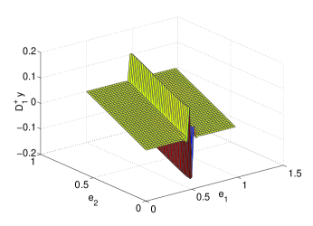
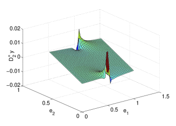
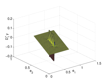
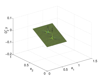
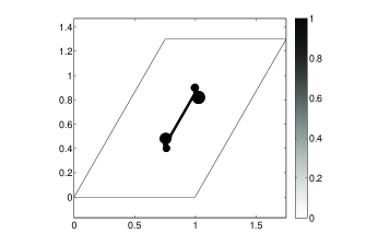
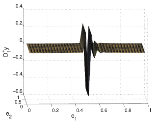
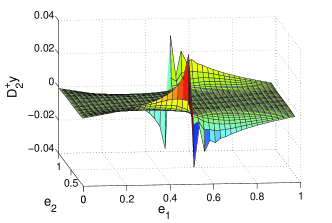
This gives an essentially two-dimensional model. We show profiles of discrete gradients Ds1+โ€‹ysuperscriptsubscript๐ทsubscript๐‘ 1๐‘ฆD_{s_{1}}^{+}y and Ds2+โ€‹ysuperscriptsubscript๐ทsubscript๐‘ 2๐‘ฆD_{s_{2}}^{+}y in Figureย 3 with M=N=20๐‘€๐‘20M=N=20. The profile of Ds1+โ€‹ysuperscriptsubscript๐ทsubscript๐‘ 1๐‘ฆD_{s_{1}}^{+}y is similar to that of the one-dimensional problem. However, if one zooms in the interface, there are some differences. To highlight the interface, for i=1,2๐‘–12i=1,2, we define

Ei={xโˆˆฮฉฮตโˆฃ|Dsiโ€‹yโ€‹(x)|โ‰ฅc0โ€‹ฮต},subscript๐ธ๐‘–conditional-set๐‘ฅsubscriptฮฉ๐œ€subscript๐ทsubscript๐‘ ๐‘–๐‘ฆ๐‘ฅsubscript๐‘0๐œ€E_{i}=\{\,x\in\Omega_{\varepsilon}\,\mid\,\lvert D_{s_{i}}y(x)\rvert\geq c_{0}\varepsilon\,\},

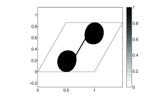
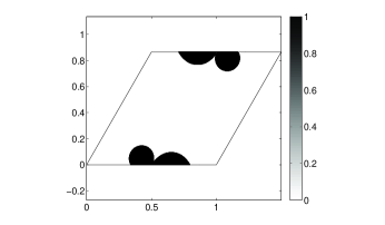
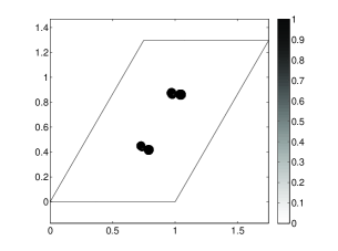
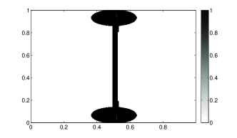
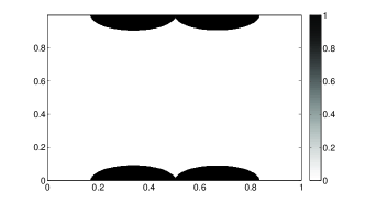
and let ฯ‡Eisubscript๐œ’subscript๐ธ๐‘–\chi_{E_{i}} be their characteristic functions. We plot ฯ‡Eiโ€‹(x)subscript๐œ’subscript๐ธ๐‘–๐‘ฅ\chi_{E_{i}}(x) in Figureย 4 with M=N=640๐‘€๐‘640M=N=640 and c0=0.04subscript๐‘00.04c_{0}=0.04. In Figureย 4(a), the width of the interface near the boundary is much wider than that in the interior domain. No interfacial layer for Ds2+โ€‹ysuperscriptsubscript๐ทsubscript๐‘ 2๐‘ฆD_{s_{2}}^{+}y is observed in Figureย 4(b). Therefore, we only measure the width of the interfacial layer for Ds1+โ€‹ysuperscriptsubscript๐ทsubscript๐‘ 1๐‘ฆD_{s_{1}}^{+}y, which is defined by

maxn{|a1|ฮต\displaystyle\max_{n}\Big{\{}|a_{1}|\varepsilon [argmaxm{x=ma1ฮต+na2ฮตโˆˆฮฉฮต|ฯ‡1(x)=1}\displaystyle\big{[}\operatorname{argmax}_{m}\{x=ma_{1}\varepsilon+na_{2}\varepsilon\in\Omega_{\varepsilon}|\chi_{1}(x)=1\}
โˆ’argminm{x=ma1ฮต+na2ฮตโˆˆฮฉฮต|ฯ‡1(x)=1}]}.\displaystyle-\operatorname{argmin}_{m}\{x=ma_{1}\varepsilon+na_{2}\varepsilon\in\Omega_{\varepsilon}|\chi_{1}(x)=1\}\big{]}\Big{\}}.

Numerical results in Tableย 1 imply that the width of the interfacial layer scales ๐’ชโ€‹(ฮต)๐’ช๐œ€\mathcal{O}(\sqrt{\varepsilon}), while the one-dimensional problem has an interfacial layer with ๐’ชโ€‹(ฮตโ€‹|lnโกฮต|)๐’ช๐œ€๐œ€\mathcal{O}(\varepsilon\lvert\ln\varepsilon\rvert) widthย [15, 2].

Refer to caption
(a) Ds1+โ€‹ysuperscriptsubscript๐ทsubscript๐‘ 1๐‘ฆD_{s_{1}}^{+}y
Refer to caption
(b) Ds2+โ€‹ysuperscriptsubscript๐ทsubscript๐‘ 2๐‘ฆD_{s_{2}}^{+}y
Figure 3. Profiles of the discrete gradients for triangular lattice with M=N=20๐‘€๐‘20M=N=20 under Dirichlet boundary condition.
Refer to caption
(a) ฯ‡E1โ€‹(x)subscript๐œ’subscript๐ธ1๐‘ฅ\chi_{E_{1}}(x)
Refer to caption
(b) ฯ‡E2โ€‹(x)subscript๐œ’subscript๐ธ2๐‘ฅ\chi_{E_{2}}(x)
Figure 4. Profiles of the characteristic functions for triangular lattice.
ฮตโ€‹(5ร—10โˆ’2)๐œ€5superscript102\varepsilon\;(5\times 10^{-2}) 20superscript202^{0} 2โˆ’1superscript212^{-1} 2โˆ’2superscript222^{-2} 2โˆ’3superscript232^{-3} 2โˆ’4superscript242^{-4} 2โˆ’5superscript252^{-5} Rate
Layer width(10โˆ’1)superscript101(10^{-1}) 3.53.53.5 2.32.32.3 1.51.51.5 0.940.940.94 0.630.630.63 0.520.520.52 0.570.570.57
Table 1. Width of the interfacial layer versus the equilibrium bond length ฮต๐œ€\varepsilon for the triangular lattice with Dirichlet boundary condition.

One may doubt the above result could be caused by the boundary condition instead of the ghost force. To clarify this issue, we enlarge the continuum region to weaken the influence of the boundary condition. We set N=3โ€‹M๐‘3๐‘€N=3M and use different equilibrium equations for different regions as in Figureย 5. Roughly speaking, along x2subscript๐‘ฅ2x_{2} direction, the original QC method is employed in the interior region, and the continuum model is padded in the outer region.
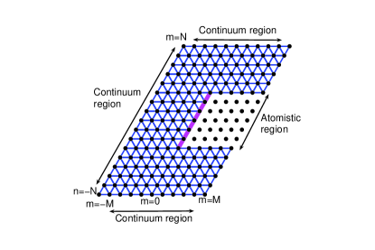
Refer to caption
Figure 5. Padding technique to remove the boundary effect.

We plot Ds1+โ€‹ysubscriptsuperscript๐ทsubscript๐‘ 1๐‘ฆD^{+}_{s_{1}}y, Ds2+โ€‹ysubscriptsuperscript๐ทsubscript๐‘ 2๐‘ฆD^{+}_{s_{2}}y, and their characteristic functions in Figureย 6 and Figureย 7. They are similar to those in Figureย 3 and Figureย 4.

Refer to caption
(a) Ds1+โ€‹ysuperscriptsubscript๐ทsubscript๐‘ 1๐‘ฆD_{s_{1}}^{+}y
Refer to caption
(b) Ds2+โ€‹ysuperscriptsubscript๐ทsubscript๐‘ 2๐‘ฆD_{s_{2}}^{+}y
Figure 6. Profiles of the discrete gradients for triangular lattice with M=20๐‘€20M=20 and padding technique under Dirichlet boundary condition.
Refer to caption
(a) ฯ‡E1โ€‹(x)subscript๐œ’subscript๐ธ1๐‘ฅ\chi_{E_{1}}(x)
Refer to caption
(b) ฯ‡E2โ€‹(x)subscript๐œ’subscript๐ธ2๐‘ฅ\chi_{E_{2}}(x)
Figure 7. Profiles of the characteristic functions for triangular lattice with padding technique.

Tableย 2 shows the width of the interfacial layer in terms of ฮต๐œ€\varepsilon. Numerical results suggest that the width of the interfacial layer is still of ๐’ชโ€‹(ฮต)๐’ช๐œ€\mathcal{O}(\sqrt{\varepsilon}\,), which is consistent with that in Tableย 1. Therefore, we conclude that the interface is caused by the ghost force instead of the boundary condition.

ฮตโ€‹(10โˆ’2)๐œ€superscript102\varepsilon(10^{-2}) 1.71.71.7 0.830.830.83 0.410.410.41 0.210.210.21 0.100.100.10 Rate
Layer width(10โˆ’2)superscript102(10^{-2}) 9.29.29.2 8.38.38.3 4.84.84.8 3.33.33.3 2.32.32.3 0.530.530.53
Table 2. Width of the interfacial layer versus the equilibrium bond length ฮต๐œ€\varepsilon by removing the effect of the boundary condition.

The QC approximation discussed in this section is quite realistic except the potential function as shown inย [15], which however seems enough to characterize the influence of the ghost force. Unfortunately, it does not seem easy to solve this model analytically as we have done inย [15] for the one-dimensional problem. In next section, we introduce a new QC method that can be solved analytically. We shall prove that this new QC method does capture the main feature of the ghost force for the triangular lattice model with a planar interface.

3. Square lattice model

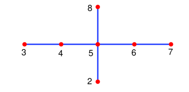
We consider the square lattice with the harmonic potential. Compared to the standard interaction range of the square lattice, we assume a special interaction range as shown in Figureย 8 (Left). Namely, the first and second neighborhood interactions in x1subscript๐‘ฅ1x_{1} direction, and the first neighborhood interaction in x2subscript๐‘ฅ2x_{2} direction are taken into account. This seemingly strange selection may be obtained from a rotated triangular lattice as in Figureย 8 (Right). If we condense the interaction of the atoms 9,4,5,11945119,4,5,11 into one atom, and the atoms 8,2,1,12821128,2,1,12 into another, then we obtain a square lattice model with the special interaction range described above, which may be the underlying reason why it can be regarded as a surrogate model. We shall show in the next two sections that this model not only captures the main features of the triangular lattice model with the QC approximation as shown in Figureย 2, but also lends itself theoretically tractable.
Refer to caption
Refer to caption
Figure 8. Interaction ranges. Left: First and second neighborhood interactions in x1subscript๐‘ฅ1x_{1} direction and first neighborhood interaction in x2subscript๐‘ฅ2x_{2} direction for square lattice; Right: First and second neighborhood interactions for triangular lattice in a rotated coordinate.

Proceeding along the same line that leads toย (2.3), we obtain the equilibrium equations for the error yโ€‹(x)๐‘ฆ๐‘ฅy(x).111We actually multiply โˆ’11-1 on both sides ofย (2.3). In the continuum region, i.e., m=โˆ’M,โ‹ฏ,โˆ’2๐‘š๐‘€โ‹ฏ2m=-M,\cdots,-2 and n=โˆ’N,โ‹ฏ,N๐‘›๐‘โ‹ฏ๐‘n=-N,\cdots,N,

12โ€‹yiโ€‹(m,n)12subscript๐‘ฆ๐‘–๐‘š๐‘›\displaystyle 12y_{i}(m,n) โˆ’yiโ€‹(m,nโˆ’1)โˆ’yiโ€‹(m,n+1)โˆ’5โ€‹yiโ€‹(mโˆ’1,n)โˆ’5โ€‹yiโ€‹(m+1,n)subscript๐‘ฆ๐‘–๐‘š๐‘›1subscript๐‘ฆ๐‘–๐‘š๐‘›15subscript๐‘ฆ๐‘–๐‘š1๐‘›5subscript๐‘ฆ๐‘–๐‘š1๐‘›\displaystyle-y_{i}(m,n-1)-y_{i}(m,n+1)-5y_{i}(m-1,n)-5y_{i}(m+1,n)
(3.1) =0,i=1,2,formulae-sequenceabsent0๐‘–12\displaystyle=0,\quad i=1,2,

and in the atomistic region, i.e., m=2,โ‹ฏ,M๐‘š2โ‹ฏ๐‘€m=2,\cdots,M and n=โˆ’N,โ‹ฏ,N๐‘›๐‘โ‹ฏ๐‘n=-N,\cdots,N,

6โ€‹yiโ€‹(m,n)6subscript๐‘ฆ๐‘–๐‘š๐‘›\displaystyle 6y_{i}(m,n) โˆ’yiโ€‹(m,nโˆ’1)โˆ’yiโ€‹(m,n+1)โˆ’yiโ€‹(mโˆ’1,n)โˆ’yiโ€‹(m+1,n)subscript๐‘ฆ๐‘–๐‘š๐‘›1subscript๐‘ฆ๐‘–๐‘š๐‘›1subscript๐‘ฆ๐‘–๐‘š1๐‘›subscript๐‘ฆ๐‘–๐‘š1๐‘›\displaystyle-y_{i}(m,n-1)-y_{i}(m,n+1)-y_{i}(m-1,n)-y_{i}(m+1,n)
(3.2) โˆ’yiโ€‹(mโˆ’2,n)โˆ’yiโ€‹(m+2,n)=0,i=1,2.formulae-sequencesubscript๐‘ฆ๐‘–๐‘š2๐‘›subscript๐‘ฆ๐‘–๐‘š2๐‘›0๐‘–12\displaystyle-y_{i}(m-2,n)-y_{i}(m+2,n)=0,\quad i=1,2.

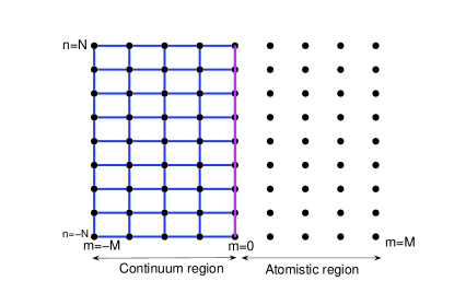
The interface between the continuum model and the atomistic model is the line m=0๐‘š0m=0 as shown in Figureย 9, and M๐‘€M is assumed to be even for simplicity. The equilibrium equations for the layers m=โˆ’1,0๐‘š10m=-1,0 and 111 are as follows.

Refer to caption
Figure 9. Square lattice with a planar interface.

For layer m=โˆ’1๐‘š1m=-1 and n=โˆ’N,โ‹ฏ,N๐‘›๐‘โ‹ฏ๐‘n=-N,\cdots,N,

252โ€‹yiโ€‹(โˆ’1,n)252subscript๐‘ฆ๐‘–1๐‘›\displaystyle\frac{25}{2}y_{i}(-1,n) โˆ’yiโ€‹(โˆ’1,nโˆ’1)โˆ’yiโ€‹(โˆ’1,n+1)โˆ’5โ€‹yiโ€‹(โˆ’2,n)โˆ’5โ€‹yiโ€‹(0,n)subscript๐‘ฆ๐‘–1๐‘›1subscript๐‘ฆ๐‘–1๐‘›15subscript๐‘ฆ๐‘–2๐‘›5subscript๐‘ฆ๐‘–0๐‘›\displaystyle-y_{i}(-1,n-1)-y_{i}(-1,n+1)-5y_{i}(-2,n)-5y_{i}(0,n)
(3.3) โˆ’12โ€‹yiโ€‹(1,n)=fi,i=1,2,formulae-sequence12subscript๐‘ฆ๐‘–1๐‘›subscript๐‘“๐‘–๐‘–12\displaystyle-\frac{1}{2}y_{i}(1,n)=f_{i},\quad i=1,2,

where f1=โˆ’ฮตsubscript๐‘“1๐œ€f_{1}=-\varepsilon and f2=0subscript๐‘“20f_{2}=0.

For layer m=0๐‘š0m=0 and n=โˆ’N,โ‹ฏ,N๐‘›๐‘โ‹ฏ๐‘n=-N,\cdots,N,

9โ€‹yiโ€‹(0,n)9subscript๐‘ฆ๐‘–0๐‘›\displaystyle 9y_{i}(0,n) โˆ’yiโ€‹(0,nโˆ’1)โˆ’yiโ€‹(0,n+1)โˆ’5โ€‹yiโ€‹(โˆ’1,n)โˆ’yiโ€‹(1,n)subscript๐‘ฆ๐‘–0๐‘›1subscript๐‘ฆ๐‘–0๐‘›15subscript๐‘ฆ๐‘–1๐‘›subscript๐‘ฆ๐‘–1๐‘›\displaystyle-y_{i}(0,n-1)-y_{i}(0,n+1)-5y_{i}(-1,n)-y_{i}(1,n)
(3.4) โˆ’yiโ€‹(2,n)=fi,i=1,2,formulae-sequencesubscript๐‘ฆ๐‘–2๐‘›subscript๐‘“๐‘–๐‘–12\displaystyle-y_{i}(2,n)=f_{i},\quad i=1,2,

where f1=2โ€‹ฮตsubscript๐‘“12๐œ€f_{1}=2\varepsilon and f2=0subscript๐‘“20f_{2}=0.

For layer m=1๐‘š1m=1 and n=โˆ’N,โ‹ฏ,N๐‘›๐‘โ‹ฏ๐‘n=-N,\cdots,N,

112โ€‹yiโ€‹(1,n)112subscript๐‘ฆ๐‘–1๐‘›\displaystyle\frac{11}{2}y_{i}(1,n) โˆ’yiโ€‹(1,nโˆ’1)โˆ’yiโ€‹(1,n+1)โˆ’yiโ€‹(0,n)โˆ’yiโ€‹(2,n)subscript๐‘ฆ๐‘–1๐‘›1subscript๐‘ฆ๐‘–1๐‘›1subscript๐‘ฆ๐‘–0๐‘›subscript๐‘ฆ๐‘–2๐‘›\displaystyle-y_{i}(1,n-1)-y_{i}(1,n+1)-y_{i}(0,n)-y_{i}(2,n)
(3.5) โˆ’12โ€‹yiโ€‹(โˆ’1,n)โˆ’yiโ€‹(3,n)=fi,i=1,2,formulae-sequence12subscript๐‘ฆ๐‘–1๐‘›subscript๐‘ฆ๐‘–3๐‘›subscript๐‘“๐‘–๐‘–12\displaystyle-\frac{1}{2}y_{i}(-1,n)-y_{i}(3,n)=f_{i},\quad i=1,2,

where f1=โˆ’ฮตsubscript๐‘“1๐œ€f_{1}=-\varepsilon and f2=0subscript๐‘“20f_{2}=0.

Observe that

y2=0.subscript๐‘ฆ20y_{2}=0.

Therefore, we only consider y1subscript๐‘ฆ1y_{1} and omit the subscript from now on.

We first impose the Dirichlet boundary condition in the x1subscript๐‘ฅ1x_{1} direction, and the periodic boundary condition in the x2subscript๐‘ฅ2x_{2} direction as

(3.6) {yโ€‹(โˆ’M,n)=yโ€‹(M,n)=yโ€‹(M+1,n)=0,n=โˆ’N,โ‹ฏ,N,yโ€‹(m,n)=yโ€‹(m,n+2โ€‹N),m=โˆ’M,โ‹ฏ,M,n=โˆ’N,โ‹ฏ,N.\left\{\begin{aligned} y(-M,n)&=y(M,n)=y(M+1,n)=0,\quad n=-N,\cdots,N,\\ y(m,n)&=y(m,n+2N),\quad m=-M,\cdots,M,n=-N,\cdots,N.\end{aligned}\right.

Similar to the triangular lattice model, it is easy to check that the square lattice model reduces to a one-dimensional chain model with the following equilibrium equations and boundary condition.

5โ€‹yโ€‹(m+1)โˆ’10โ€‹yโ€‹(m)+5โ€‹yโ€‹(mโˆ’1)5๐‘ฆ๐‘š110๐‘ฆ๐‘š5๐‘ฆ๐‘š1\displaystyle 5y(m+1)-10y(m)+5y(m-1) =0,m=โˆ’M+1,โ‹ฏ,โˆ’2,formulae-sequenceabsent0๐‘š๐‘€1โ‹ฏ2\displaystyle=0,\;m=-M+1,\cdots,-2,
yโ€‹(m+2)+yโ€‹(m+1)โˆ’4โ€‹yโ€‹(m)+yโ€‹(mโˆ’1)+yโ€‹(mโˆ’2)๐‘ฆ๐‘š2๐‘ฆ๐‘š14๐‘ฆ๐‘š๐‘ฆ๐‘š1๐‘ฆ๐‘š2\displaystyle y(m+2)+y(m+1)-4y(m)+y(m-1)+y(m-2) =0,m=2,โ‹ฏ,Mโˆ’1.formulae-sequenceabsent0๐‘š2โ‹ฏ๐‘€1\displaystyle=0,\;m=2,\cdots,M-1.

The equations for the interface are

{12โ€‹yโ€‹(1)+5โ€‹yโ€‹(0)โˆ’212โ€‹yโ€‹(โˆ’1)+5โ€‹yโ€‹(โˆ’2)=ฮต,yโ€‹(2)+yโ€‹(1)โˆ’7โ€‹yโ€‹(0)+5โ€‹yโ€‹(โˆ’1)=โˆ’2โ€‹ฮต,yโ€‹(3)+yโ€‹(2)โˆ’72โ€‹yโ€‹(1)+yโ€‹(0)+12โ€‹yโ€‹(โˆ’1)=ฮต.\left\{\begin{aligned} \dfrac{1}{2}y(1)+5y(0)-\dfrac{21}{2}y(-1)+5y(-2)&=\varepsilon,\\ y(2)+y(1)-7y(0)+5y(-1)&=-2\varepsilon,\\ y(3)+y(2)-\dfrac{7}{2}y(1)+y(0)+\dfrac{1}{2}y(-1)&=\varepsilon.\end{aligned}\right.

The boundary condition is

yโ€‹(โˆ’M)=yโ€‹(M)=yโ€‹(M+1)=0.๐‘ฆ๐‘€๐‘ฆ๐‘€๐‘ฆ๐‘€10y(-M)=y(M)=y(M+1)=0.

It is clear that the above model is exactly the same as that has been studied inย [15], which can also be obtained from the one-dimensional modelย (2.4) with k1=k2=1subscript๐‘˜1subscript๐‘˜21k_{1}=k_{2}=1.

Therefore, we impose the Dirichlet boundary condition in both x1subscript๐‘ฅ1x_{1} and x2subscript๐‘ฅ2x_{2} directions as follows.

(3.7) {yโ€‹(โˆ’M,n)=yโ€‹(M,n)=yโ€‹(M+1,n)=0,n=โˆ’N,โ‹ฏ,N,yโ€‹(m,โˆ’N)=yโ€‹(m,N)=0,m=โˆ’M,โ‹ฏ,M.\left\{\begin{aligned} y(-M,n)&=y(M,n)=y(M+1,n)=0,&&n=-N,\cdots,N,\\ y(m,-N)&=y(m,N)=0,&&m=-M,\cdots,M.\end{aligned}\right.

Choosing M=N=20๐‘€๐‘20M=N=20, we show profiles of the discrete gradients Ds1+โ€‹ysuperscriptsubscript๐ทsubscript๐‘ 1๐‘ฆD_{s_{1}}^{+}y and Ds2+โ€‹ysuperscriptsubscript๐ทsubscript๐‘ 2๐‘ฆD_{s_{2}}^{+}y in Figureย 10. The feature is similar to that of the triangular lattice model. To highlight the interface, we plot the characteristic functions ฯ‡E1subscript๐œ’subscript๐ธ1\chi_{E_{1}} and ฯ‡E2subscript๐œ’subscript๐ธ2\chi_{E_{2}} in Figureย 11 with M=N=320๐‘€๐‘320M=N=320 and c0=0.04subscript๐‘00.04c_{0}=0.04.

Refer to caption
(a) Ds1+โ€‹ysuperscriptsubscript๐ทsubscript๐‘ 1๐‘ฆD_{s_{1}}^{+}y
Refer to caption
(b) Ds2+โ€‹ysuperscriptsubscript๐ทsubscript๐‘ 2๐‘ฆD_{s_{2}}^{+}y
Figure 10. Profiles of the discrete gradients of y๐‘ฆy for square lattice with M=N=20๐‘€๐‘20M=N=20 under Dirichlet boundary condition.
Refer to caption
(a) ฯ‡E1โ€‹(x)subscript๐œ’subscript๐ธ1๐‘ฅ\chi_{E_{1}}(x)
Refer to caption
(b) ฯ‡E2โ€‹(x)subscript๐œ’subscript๐ธ2๐‘ฅ\chi_{E_{2}}(x)
Figure 11. Profiles of the characteristic functions for square lattice.

We report the width of the interfacial layer in Tableย 3. It is clear that the width of the interfacial layer is of ๐’ชโ€‹(ฮต)๐’ช๐œ€\mathcal{O}(\sqrt{\varepsilon}\,), which is consistent with that of the triangular lattice. In ยงย 5, we shall prove this fact.

ฮตโ€‹(5ร—10โˆ’2)๐œ€5superscript102\varepsilon\;(5\times 10^{-2}) 20superscript202^{0} 2โˆ’1superscript212^{-1} 2โˆ’2superscript222^{-2} 2โˆ’3superscript232^{-3} 2โˆ’4superscript242^{-4} Rate
Layer width(10โˆ’1)superscript101\;(10^{-1}) 888 5.55.55.5 3.633.633.63 2.562.562.56 1.841.841.84 0.530.530.53
Table 3. Width of interfacial layer versus the equilibrium bond length ฮต๐œ€\varepsilon for square lattice.

4. Exact solution for the square lattice model

To find the exact solution of the QC approximationย (3.1) โ€“ (3.5) with Dirichlet boundary conditionย (3.7), we follow the approach inย [15]: firstly, we find the general expression for the solution of the continuum equation and the atomistic equation by separation of variables ansatz, with certain unspecified constants; secondly, we use the equations around the interface to determine these constants. The next lemma gives the general expression of the solution.

Lemma 4.1.

For m=โˆ’M,โ‹ฏ,โˆ’1๐‘š๐‘€โ‹ฏ1m=-M,\cdots,-1 and n=โˆ’N,โ‹ฏ,N๐‘›๐‘โ‹ฏ๐‘n=-N,\cdots,N, we have

(4.1) yโ€‹(m,n)=โˆ‘k=12โ€‹Nโˆ’1akโ€‹sinhโก[(M+m)โ€‹ฮฑk]โ€‹sinโกkโ€‹ฯ€2โ€‹Nโ€‹(N+n),๐‘ฆ๐‘š๐‘›superscriptsubscript๐‘˜12๐‘1subscript๐‘Ž๐‘˜๐‘€๐‘šsubscript๐›ผ๐‘˜๐‘˜๐œ‹2๐‘๐‘๐‘›y(m,n)=\sum_{k=1}^{2N-1}a_{k}\sinh[(M+m)\alpha_{k}]\sin\dfrac{k\pi}{2N}(N+n),

where

coshโกฮฑk=1+ฮปk5,ฮปk=2โ€‹sin2โกkโ€‹ฯ€4โ€‹N.formulae-sequencesubscript๐›ผ๐‘˜1subscript๐œ†๐‘˜5subscript๐œ†๐‘˜2superscript2๐‘˜๐œ‹4๐‘\cosh\alpha_{k}=1+\dfrac{\lambda_{k}}{5},\qquad\lambda_{k}=2\sin^{2}\dfrac{k\pi}{4N}.

For m=0,โ‹ฏ,M๐‘š0โ‹ฏ๐‘€m=0,\cdots,M and n=โˆ’N,โ‹ฏ,N๐‘›๐‘โ‹ฏ๐‘n=-N,\cdots,N, we have

(4.2) yโ€‹(m,n)=โˆ‘k=12โ€‹Nโˆ’1(bkโ€‹(โˆ’1)mโ€‹Fmโ€‹(ฮณk,ฮดk)+ckโ€‹fmโ€‹(ฮณk,ฮดk))โ€‹sinโกkโ€‹ฯ€2โ€‹Nโ€‹(N+n),๐‘ฆ๐‘š๐‘›superscriptsubscript๐‘˜12๐‘1subscript๐‘๐‘˜superscript1๐‘šsubscript๐น๐‘šsubscript๐›พ๐‘˜subscript๐›ฟ๐‘˜subscript๐‘๐‘˜subscript๐‘“๐‘šsubscript๐›พ๐‘˜subscript๐›ฟ๐‘˜๐‘˜๐œ‹2๐‘๐‘๐‘›y(m,n)=\sum_{k=1}^{2N-1}\left(b_{k}\bigl{(}-1\bigr{)}^{m}F_{m}(\gamma_{k},\delta_{k})+c_{k}f_{m}(\gamma_{k},\delta_{k})\right)\sin\dfrac{k\pi}{2N}(N+n),

where

(4.3) coshโกฮณk=1+25+8โ€‹ฮปk4,coshโกฮดk=โˆ’1+25+8โ€‹ฮปk4,formulae-sequencesubscript๐›พ๐‘˜1258subscript๐œ†๐‘˜4subscript๐›ฟ๐‘˜1258subscript๐œ†๐‘˜4\cosh\gamma_{k}=\dfrac{1+\sqrt{25+8\lambda_{k}}}{4},\quad\cosh\delta_{k}=\dfrac{-1+\sqrt{25+8\lambda_{k}}}{4},

and

(4.4) {Fmโ€‹(ฮณ,ฮด)=sinhโก[(M+1โˆ’m)โ€‹ฮณ]+sinhโก[(Mโˆ’m)โ€‹ฮณ]โ€‹coshโกฮดcoshโกฮณ+coshโกฮดโˆ’(โˆ’1)mโ€‹coshโก[(Mโˆ’m)โ€‹ฮด]โ€‹sinhโกฮณcoshโกฮณ+coshโกฮด,fmโ€‹(ฮณ,ฮด)=Fmโ€‹(ฮด,ฮณ).\left\{\begin{aligned} F_{m}(\gamma,\delta)&=\dfrac{\sinh[(M+1-m)\gamma]+\sinh[(M-m)\gamma]\cosh\delta}{\cosh\gamma+\cosh\delta}\\ &\quad-\bigl{(}-1\bigr{)}^{m}\dfrac{\cosh[(M-m)\delta]\sinh\gamma}{\cosh\gamma+\cosh\delta},\\ f_{m}(\gamma,\delta)&=F_{m}(\delta,\gamma).\end{aligned}\right.

The coefficients bksubscript๐‘๐‘˜b_{k} and cksubscript๐‘๐‘˜c_{k} are parameters to be determined; See; cf.,ย (4.13).

Proof.

By separation of variables, we getย (4.1).

The explicit expression for the solution of the atomistic model can also be obtained by separation of variables ansatz. Substituting yโ€‹(m,n)=fโ€‹(m)โ€‹gโ€‹(n)๐‘ฆ๐‘š๐‘›๐‘“๐‘š๐‘”๐‘›y(m,n)=f(m)g(n) intoย (3.2), we get

โˆ‘i=โˆ’22[fโ€‹(m+i)โˆ’fโ€‹(m)]โ€‹gโ€‹(n)+โˆ‘i=โˆ’11[gโ€‹(n+i)โˆ’gโ€‹(n)]โ€‹fโ€‹(m)=0.superscriptsubscript๐‘–22delimited-[]๐‘“๐‘š๐‘–๐‘“๐‘š๐‘”๐‘›superscriptsubscript๐‘–11delimited-[]๐‘”๐‘›๐‘–๐‘”๐‘›๐‘“๐‘š0\sum_{i=-2}^{2}[f(m+i)-f(m)]g(n)+\sum_{i=-1}^{1}[g(n+i)-g(n)]f(m)=0.

Byย (3.7), we have

gโ€‹(โˆ’N)=gโ€‹(N)=0andfโ€‹(M)=fโ€‹(M+1)=0.formulae-sequence๐‘”๐‘๐‘”๐‘0and๐‘“๐‘€๐‘“๐‘€10g(-N)=g(N)=0\quad\text{and}\quad f(M)=f(M+1)=0.

We write the above equation as

โˆ‘i=โˆ’22[fโ€‹(m+i)โˆ’fโ€‹(m)]fโ€‹(m)+โˆ‘i=โˆ’11[gโ€‹(n+i)โˆ’gโ€‹(n)]gโ€‹(n)=0.superscriptsubscript๐‘–22delimited-[]๐‘“๐‘š๐‘–๐‘“๐‘š๐‘“๐‘šsuperscriptsubscript๐‘–11delimited-[]๐‘”๐‘›๐‘–๐‘”๐‘›๐‘”๐‘›0\dfrac{\sum_{i=-2}^{2}[f(m+i)-f(m)]}{f(m)}+\dfrac{\sum_{i=-1}^{1}[g(n+i)-g(n)]}{g(n)}=0.

For ฮปโˆˆโ„๐œ†โ„\lambda\in\mathbb{R}, we get

{gโ€‹(n+1)+(2โ€‹ฮปโˆ’2)โ€‹gโ€‹(n)+gโ€‹(nโˆ’1)=0,fโ€‹(m+2)+fโ€‹(m+1)โˆ’(4+2โ€‹ฮป)โ€‹fโ€‹(m)+fโ€‹(mโˆ’1)+fโ€‹(mโˆ’2)=0.\left\{\begin{aligned} g(n+1)+(2\lambda-2)g(n)+g(n-1)&=0,\\ f(m+2)+f(m+1)-(4+2\lambda)f(m)+f(m-1)+f(m-2)&=0.\end{aligned}\right.

Using the boundary condition for g๐‘”g, i.e., gโ€‹(N)=gโ€‹(โˆ’N)=0๐‘”๐‘๐‘”๐‘0g(N)=g(-N)=0, we have, for any cโˆˆโ„๐‘โ„c\in\mathbb{R},

gโ€‹(n)=cโ€‹sinโกkโ€‹ฯ€2โ€‹Nโ€‹(n+N)andฮป=2โ€‹sin2โกkโ€‹ฯ€4โ€‹N.formulae-sequence๐‘”๐‘›๐‘๐‘˜๐œ‹2๐‘๐‘›๐‘and๐œ†2superscript2๐‘˜๐œ‹4๐‘g(n)=c\sin\dfrac{k\pi}{2N}(n+N)\quad\text{and}\quad\lambda=2\sin^{2}\dfrac{k\pi}{4N}.

The characteristic equation for fโ€‹(m)๐‘“๐‘šf(m) is:

t2+tโˆ’2+t+tโˆ’1โˆ’2โ€‹(ฮป+2)=0.superscript๐‘ก2superscript๐‘ก2๐‘กsuperscript๐‘ก12๐œ†20t^{2}+t^{-2}+t+t^{-1}-2(\lambda+2)=0.

Denote the roots of the above equation by t1,โ‹ฏ,t4subscript๐‘ก1โ‹ฏsubscript๐‘ก4t_{1},\cdots,t_{4}. It is clear that

t1=โˆ’eฮณ,t2=โˆ’eโˆ’ฮณ,t3=eฮด,t4=eโˆ’ฮด,formulae-sequencesubscript๐‘ก1superscript๐‘’๐›พformulae-sequencesubscript๐‘ก2superscript๐‘’๐›พformulae-sequencesubscript๐‘ก3superscript๐‘’๐›ฟsubscript๐‘ก4superscript๐‘’๐›ฟt_{1}=-e^{\gamma},\;t_{2}=-e^{-\gamma},\;t_{3}=e^{\delta},\;t_{4}=e^{-\delta},

with

2โ€‹coshโกฮณ2๐›พ\displaystyle 2\cosh\gamma =โˆ’s1,absentsubscript๐‘ 1\displaystyle=-s_{1}, s1=โˆ’1โˆ’25+8โ€‹ฮป2,subscript๐‘ 11258๐œ†2\displaystyle s_{1}=\dfrac{-1-\sqrt{25+8\lambda}}{2},
2โ€‹coshโกฮด2๐›ฟ\displaystyle 2\cosh\delta =s2,absentsubscript๐‘ 2\displaystyle=s_{2}, s2=โˆ’1+25+8โ€‹ฮป2.subscript๐‘ 21258๐œ†2\displaystyle s_{2}=\dfrac{-1+\sqrt{25+8\lambda}}{2}.

This leads to

fโ€‹(m)๐‘“๐‘š\displaystyle f(m) =aโ€‹(โˆ’1)mโ€‹sinhโก[(Mโˆ’m)โ€‹ฮณ]+bโ€‹(โˆ’1)mโ€‹coshโก[(Mโˆ’m)โ€‹ฮณ]absent๐‘Žsuperscript1๐‘š๐‘€๐‘š๐›พ๐‘superscript1๐‘š๐‘€๐‘š๐›พ\displaystyle=a\bigl{(}-1\bigr{)}^{m}\sinh[(M-m)\gamma]+b\bigl{(}-1\bigr{)}^{m}\cosh[(M-m)\gamma]
+cโ€‹sinhโก[(Mโˆ’m)โ€‹ฮด]+dโ€‹coshโก[(Mโˆ’m)โ€‹ฮด]๐‘๐‘€๐‘š๐›ฟ๐‘‘๐‘€๐‘š๐›ฟ\displaystyle\quad+c\sinh[(M-m)\delta]+d\cosh[(M-m)\delta]

with constants a,b,c๐‘Ž๐‘๐‘a,b,c and d๐‘‘d that will be determined by the following conditions

fโ€‹(M)=fโ€‹(M+1)=0.๐‘“๐‘€๐‘“๐‘€10f(M)=f(M+1)=0.

Since M๐‘€M is even, by fโ€‹(M)=0๐‘“๐‘€0f(M)=0, we obtain

b=โˆ’d.๐‘๐‘‘b=-d.

By fโ€‹(M+1)=0๐‘“๐‘€10f(M+1)=0, we obtain

aโ€‹sinhโกฮณโˆ’cโ€‹sinhโกฮดโˆ’bโ€‹(coshโกฮณ+cosโกฮด)=0.๐‘Ž๐›พ๐‘๐›ฟ๐‘๐›พ๐›ฟ0a\sinh\gamma-c\sinh\delta-b(\cosh\gamma+\cos\delta)=0.

Therefore,

b=aโ€‹sinhโกฮณโˆ’cโ€‹sinhโกฮดcoshโกฮณ+coshโกฮด.๐‘๐‘Ž๐›พ๐‘๐›ฟ๐›พ๐›ฟb=\dfrac{a\sinh\gamma-c\sinh\delta}{\cosh\gamma+\cosh\delta}.

We write fโ€‹(m)๐‘“๐‘šf(m) as

fโ€‹(m)๐‘“๐‘š\displaystyle f(m) =aโ€‹(โˆ’1)mโ€‹sinhโก[(Mโˆ’m)โ€‹ฮณ]+cโ€‹sinhโก[(Mโˆ’m)โ€‹ฮด]absent๐‘Žsuperscript1๐‘š๐‘€๐‘š๐›พ๐‘๐‘€๐‘š๐›ฟ\displaystyle=a\bigl{(}-1\bigr{)}^{m}\sinh[(M-m)\gamma]+c\sinh[(M-m)\delta]
+aโ€‹sinhโกฮณโˆ’cโ€‹sinhโกฮดcoshโกฮณ+coshโกฮดโ€‹{(โˆ’1)mโ€‹coshโก[(Mโˆ’m)โ€‹ฮณ]โˆ’coshโก[(Mโˆ’m)โ€‹ฮด]}.๐‘Ž๐›พ๐‘๐›ฟ๐›พ๐›ฟsuperscript1๐‘š๐‘€๐‘š๐›พ๐‘€๐‘š๐›ฟ\displaystyle\quad+\dfrac{a\sinh\gamma-c\sinh\delta}{\cosh\gamma+\cosh\delta}\Bigl{\{}\bigl{(}-1\bigr{)}^{m}\cosh[(M-m)\gamma]-\cosh[(M-m)\delta]\Bigr{\}}.

It is easy to rewrite fโ€‹(m)๐‘“๐‘šf(m) into a symmetrical form

fโ€‹(m)=aโ€‹(โˆ’1)mโ€‹Fmโ€‹(ฮณ,ฮด)+cโ€‹Fmโ€‹(ฮด,ฮณ),๐‘“๐‘š๐‘Žsuperscript1๐‘šsubscript๐น๐‘š๐›พ๐›ฟ๐‘subscript๐น๐‘š๐›ฟ๐›พf(m)=a\bigl{(}-1\bigr{)}^{m}F_{m}(\gamma,\delta)+cF_{m}(\delta,\gamma),

where Fmโ€‹(ฮณ,ฮด)subscript๐น๐‘š๐›พ๐›ฟF_{m}(\gamma,\delta) is given inย (4.4), this givesย (4.3). โˆŽ

Remark 4.2.

The exact solution based on the series expansion is common in finite difference. We refer toย [13] andย [8] for a thorough discussion.

Next we use the interfacial equationsย (3.3) โ€“ (3.5) to determine the coefficients ak,bksubscript๐‘Ž๐‘˜subscript๐‘๐‘˜a_{k},b_{k} and cksubscript๐‘๐‘˜c_{k}. Denote

ycbโ€‹(m,n)subscript๐‘ฆcb๐‘š๐‘›\displaystyle y_{\text{cb}}(m,n) =yโ€‹(m,n)โˆ’Mโ‰คmโ‰คโˆ’1,โˆ’Nโ‰คnโ‰คN,formulae-sequenceformulae-sequenceabsent๐‘ฆ๐‘š๐‘›๐‘€๐‘š1๐‘๐‘›๐‘\displaystyle=y(m,n)\qquad-M\leq m\leq-1,-N\leq n\leq N,
yatโ€‹(m,n)subscript๐‘ฆat๐‘š๐‘›\displaystyle y_{\text{at}}(m,n) =yโ€‹(m,n)0โ‰คmโ‰คM,โˆ’Nโ‰คnโ‰คN.formulae-sequenceformulae-sequenceabsent๐‘ฆ๐‘š๐‘›0๐‘š๐‘€๐‘๐‘›๐‘\displaystyle=y(m,n)\qquad 0\leq m\leq M,-N\leq n\leq N.

Though ycbsubscript๐‘ฆcby_{\text{cb}} and yatsubscript๐‘ฆaty_{\text{at}} are only defined piecewisely, they actually admit a trivial extension for any (m,n)โˆˆโ„ค2๐‘š๐‘›superscriptโ„ค2(m,n)\in\mathbb{Z}^{2} as

(4.5) โ„ฑฮตโ€‹[ycb]โ€‹(m,n)=0,โ„ฑatโ€‹[yat]โ€‹(m,n)=0,for(m,n)โˆˆโ„ค2,formulae-sequencesubscriptโ„ฑ๐œ€delimited-[]subscript๐‘ฆcb๐‘š๐‘›0formulae-sequencesubscriptโ„ฑatdelimited-[]subscript๐‘ฆat๐‘š๐‘›0for๐‘š๐‘›superscriptโ„ค2\mathcal{F}_{\varepsilon}[y_{\text{cb}}](m,n)=0,\qquad\mathcal{F}_{\text{at}}[y_{\text{at}}](m,n)=0,\qquad\text{for}\quad(m,n)\in\mathbb{Z}^{2},

where

โ„ฑฮตโ€‹[y]โ€‹(m,n)subscriptโ„ฑ๐œ€delimited-[]๐‘ฆ๐‘š๐‘›\displaystyle\mathcal{F}_{\varepsilon}[y](m,n) โ‰ก12โ€‹yโ€‹(m,n)โˆ’yโ€‹(m,nโˆ’1)โˆ’yโ€‹(m,n+1)โˆ’5โ€‹yโ€‹(mโˆ’1,n)โˆ’5โ€‹yโ€‹(m+1,n),absent12๐‘ฆ๐‘š๐‘›๐‘ฆ๐‘š๐‘›1๐‘ฆ๐‘š๐‘›15๐‘ฆ๐‘š1๐‘›5๐‘ฆ๐‘š1๐‘›\displaystyle\equiv 12y(m,n)-y(m,n-1)-y(m,n+1)-5y(m-1,n)-5y(m+1,n),
โ„ฑatโ€‹[y]โ€‹(m,n)subscriptโ„ฑatdelimited-[]๐‘ฆ๐‘š๐‘›\displaystyle\mathcal{F}_{\text{at}}[y](m,n) โ‰ก6โ€‹yโ€‹(m,n)โˆ’yโ€‹(m,nโˆ’1)โˆ’yโ€‹(m,n+1)โˆ’yโ€‹(mโˆ’1,n)โˆ’yโ€‹(m+1,n)absent6๐‘ฆ๐‘š๐‘›๐‘ฆ๐‘š๐‘›1๐‘ฆ๐‘š๐‘›1๐‘ฆ๐‘š1๐‘›๐‘ฆ๐‘š1๐‘›\displaystyle\equiv 6y(m,n)-y(m,n-1)-y(m,n+1)-y(m-1,n)-y(m+1,n)
โˆ’yโ€‹(mโˆ’2,n)โˆ’yโ€‹(m+2,n).๐‘ฆ๐‘š2๐‘›๐‘ฆ๐‘š2๐‘›\displaystyle\quad-y(m-2,n)-y(m+2,n).

This observation is crucial to simplify the equations around the interface.

The equation for m=โˆ’1๐‘š1m=-1 changes to

โ„ฑฮตโ€‹[ycbโ€‹(1ยฏ,n)]+5โ€‹(ycbโˆ’yat)โ€‹(0,n)+12โ€‹(ycbโ€‹(1ยฏ,n)โˆ’yatโ€‹(1,n))=โˆ’ฮต.subscriptโ„ฑ๐œ€delimited-[]subscript๐‘ฆcbยฏ1๐‘›5subscript๐‘ฆcbsubscript๐‘ฆat0๐‘›12subscript๐‘ฆcbยฏ1๐‘›subscript๐‘ฆat1๐‘›๐œ€\mathcal{F}_{\varepsilon}[y_{\text{cb}}(\bar{1},n)]+5(y_{\text{cb}}-y_{\text{at}})(0,n)+\frac{1}{2}\Bigl{(}y_{\text{cb}}(\bar{1},n)-y_{\text{at}}(1,n)\Bigr{)}=-\varepsilon.

Using

โ„ฑฮตโ€‹[ycbโ€‹(1ยฏ,n)]=0,subscriptโ„ฑ๐œ€delimited-[]subscript๐‘ฆcbยฏ1๐‘›0\mathcal{F}_{\varepsilon}[y_{\text{cb}}(\bar{1},n)]=0,

we have

(4.6) 5โ€‹(ycbโˆ’yat)โ€‹(0,n)+12โ€‹(ycbโ€‹(1ยฏ,n)โˆ’yatโ€‹(1,n))=โˆ’ฮต.5subscript๐‘ฆcbsubscript๐‘ฆat0๐‘›12subscript๐‘ฆcbยฏ1๐‘›subscript๐‘ฆat1๐‘›๐œ€5(y_{\text{cb}}-y_{\text{at}})(0,n)+\frac{1}{2}\Bigl{(}y_{\text{cb}}(\bar{1},n)-y_{\text{at}}(1,n)\Bigr{)}=-\varepsilon.

Proceeding in the same fashion, we get

(4.7) yatโ€‹(1ยฏ,n)โˆ’12โ€‹yatโ€‹(1,n)โˆ’12โ€‹ycbโ€‹(1ยฏ,n)=โˆ’ฮต,subscript๐‘ฆatยฏ1๐‘›12subscript๐‘ฆat1๐‘›12subscript๐‘ฆcbยฏ1๐‘›๐œ€\displaystyle y_{\text{at}}(\bar{1},n)-\frac{1}{2}y_{\text{at}}(1,n)-\frac{1}{2}y_{\text{cb}}(\bar{1},n)=-\varepsilon,
(4.8) 3โ€‹yatโ€‹(0,n)+yatโ€‹(1ยฏ,n)+yatโ€‹(2ยฏ,n)โˆ’5โ€‹ycbโ€‹(1ยฏ,n)=2โ€‹ฮต.3subscript๐‘ฆat0๐‘›subscript๐‘ฆatยฏ1๐‘›subscript๐‘ฆatยฏ2๐‘›5subscript๐‘ฆcbยฏ1๐‘›2๐œ€\displaystyle 3y_{\text{at}}(0,n)+y_{\text{at}}(\bar{1},n)+y_{\text{at}}(\bar{2},n)-5y_{\text{cb}}(\bar{1},n)=2\varepsilon.

In what follows, we use the above simplified interfacial equations and the representation formulas to determine ak,bksubscript๐‘Ž๐‘˜subscript๐‘๐‘˜a_{k},b_{k} and cksubscript๐‘๐‘˜c_{k}.

Subtractingย (4.7) fromย (4.6), we obtain

5โ€‹ycbโ€‹(0,n)+ycbโ€‹(1ยฏ,n)=5โ€‹yatโ€‹(0,n)+yatโ€‹(1ยฏ,n).5subscript๐‘ฆcb0๐‘›subscript๐‘ฆcbยฏ1๐‘›5subscript๐‘ฆat0๐‘›subscript๐‘ฆatยฏ1๐‘›5y_{\text{cb}}(0,n)+y_{\text{cb}}(\bar{1},n)=5y_{\text{at}}(0,n)+y_{\text{at}}(\bar{1},n).

Substitutingย (4.1) andย (4.2) into the above equation, we get

(4.9) ak=bkโ€‹(5โ€‹F0โˆ’F1ยฏ)โ€‹(ฮณk,ฮดk)+ckโ€‹(5โ€‹f0+f1ยฏ)โ€‹(ฮณk,ฮดk)5โ€‹sinhโก[Mโ€‹ฮฑk]+sinhโก[(Mโˆ’1)โ€‹ฮฑk].subscript๐‘Ž๐‘˜subscript๐‘๐‘˜5subscript๐น0subscript๐นยฏ1subscript๐›พ๐‘˜subscript๐›ฟ๐‘˜subscript๐‘๐‘˜5subscript๐‘“0subscript๐‘“ยฏ1subscript๐›พ๐‘˜subscript๐›ฟ๐‘˜5๐‘€subscript๐›ผ๐‘˜๐‘€1subscript๐›ผ๐‘˜a_{k}=\dfrac{b_{k}(5F_{0}-F_{\bar{1}})(\gamma_{k},\delta_{k})+c_{k}(5f_{0}+f_{\bar{1}})(\gamma_{k},\delta_{k})}{5\sinh[M\alpha_{k}]+\sinh[(M-1)\alpha_{k}]}.

Substitutingย (4.1) andย (4.2) intoย (4.7), we get

โˆ‘k=12โ€‹Nโˆ’1โ„“kโ€‹sinโก[kโ€‹ฯ€2โ€‹Nโ€‹(n+N)]=โˆ’2โ€‹ฮตsuperscriptsubscript๐‘˜12๐‘1subscriptโ„“๐‘˜๐‘˜๐œ‹2๐‘๐‘›๐‘2๐œ€\sum_{k=1}^{2N-1}\ell_{k}\sin\left[\dfrac{k\pi}{2N}(n+N)\right]=-2\varepsilon

with

โ„“k=โˆ’sinhโก[(Mโˆ’1)โ€‹ฮฑk]โ€‹ak+(โˆ’2โ€‹F1ยฏ+F1)โ€‹(ฮณk,ฮดk)โ€‹bk+(2โ€‹f1ยฏโˆ’f1)โ€‹(ฮณk,ฮดk)โ€‹ck.subscriptโ„“๐‘˜๐‘€1subscript๐›ผ๐‘˜subscript๐‘Ž๐‘˜2subscript๐นยฏ1subscript๐น1subscript๐›พ๐‘˜subscript๐›ฟ๐‘˜subscript๐‘๐‘˜2subscript๐‘“ยฏ1subscript๐‘“1subscript๐›พ๐‘˜subscript๐›ฟ๐‘˜subscript๐‘๐‘˜\ell_{k}=-\sinh[(M-1)\alpha_{k}]a_{k}+(-2F_{\bar{1}}+F_{1})(\gamma_{k},\delta_{k})b_{k}+(2f_{\bar{1}}-f_{1})(\gamma_{k},\delta_{k})c_{k}.

Using the discrete Fourier transform, we get

โ„“k=2ร—(โˆ’2โ€‹ฮต)2โ€‹Nโˆ’1+1โˆ‘j=12โ€‹Nโˆ’1sinkโ€‹ฯ€โ€‹j2โ€‹N={โˆ’2โ€‹ฮตNโ€‹cotโกkโ€‹ฯ€4โ€‹N,ifย kย is odd,ย 0,ifย kย is even.\ell_{k}=\dfrac{2\times(-2\varepsilon)}{2N-1+1}\sum_{j=1}^{2N-1}\sin\dfrac{k\pi j}{2N}=\left\{\begin{aligned} -\dfrac{2\varepsilon}{N}\cot{\dfrac{k\pi}{4N}},&\quad\text{if $k$ is odd, }\\ 0,&\quad\text{if $k$ is even.}\end{aligned}\right.

This leads to

(4.10) Pkโ€‹bk+pkโ€‹ck=โ„“k,subscript๐‘ƒ๐‘˜subscript๐‘๐‘˜subscript๐‘๐‘˜subscript๐‘๐‘˜subscriptโ„“๐‘˜P_{k}b_{k}+p_{k}c_{k}=\ell_{k},

where

(4.11) {Pk=[โˆ’2โ€‹F1ยฏ+F1โˆ’ฯkโ€‹(โˆ’F1ยฏ+5โ€‹F0)]โ€‹(ฮณk,ฮดk),pk=[2โ€‹f1ยฏโˆ’f1โˆ’ฯkโ€‹(f1ยฏ+5โ€‹f0)]โ€‹(ฮณk,ฮดk),ฯk=sinhโก[(Mโˆ’1)โ€‹ฮฑk]5โ€‹sinhโก[Mโ€‹ฮฑk]+sinhโก[(Mโˆ’1)โ€‹ฮฑk].\left\{\begin{aligned} P_{k}&=[-2F_{\bar{1}}+F_{1}-\rho_{k}(-F_{\bar{1}}+5F_{0})](\gamma_{k},\delta_{k}),\\ p_{k}&=[2f_{\bar{1}}-f_{1}-\rho_{k}(f_{\bar{1}}+5f_{0})](\gamma_{k},\delta_{k}),\\ \rho_{k}&=\dfrac{\sinh[(M-1)\alpha_{k}]}{5\sinh[M\alpha_{k}]+\sinh[(M-1)\alpha_{k}]}.\end{aligned}\right.

Usingย (4.7) andย (4.8) to eliminate ycbโ€‹(1ยฏ,n)subscript๐‘ฆcbยฏ1๐‘›y_{\text{cb}}(\bar{1},n), we obtain

3โ€‹yatโ€‹(0,n)โˆ’9โ€‹yatโ€‹(1ยฏ,n)+yatโ€‹(2ยฏ,n)+5โ€‹yatโ€‹(1,n)=12โ€‹ฮต.3subscript๐‘ฆat0๐‘›9subscript๐‘ฆatยฏ1๐‘›subscript๐‘ฆatยฏ2๐‘›5subscript๐‘ฆat1๐‘›12๐œ€3y_{\text{at}}(0,n)-9y_{\text{at}}(\bar{1},n)+y_{\text{at}}(\bar{2},n)+5y_{\text{at}}(1,n)=12\varepsilon.

The coefficients bksubscript๐‘๐‘˜b_{k} and cksubscript๐‘๐‘˜c_{k} satisfy

(4.12) Rkโ€‹bk+rkโ€‹ck=โˆ’6โ€‹โ„“k,subscript๐‘…๐‘˜subscript๐‘๐‘˜subscript๐‘Ÿ๐‘˜subscript๐‘๐‘˜6subscriptโ„“๐‘˜R_{k}b_{k}+r_{k}c_{k}=-6\ell_{k},

where

{Rk=(3โ€‹F0+9โ€‹F1ยฏ+F2ยฏโˆ’5โ€‹F1)โ€‹(ฮณk,ฮดk),rk=(3โ€‹f0โˆ’9โ€‹f1ยฏ+f2ยฏ+5โ€‹f1)โ€‹(ฮณk,ฮดk).\left\{\begin{aligned} R_{k}&=(3F_{0}+9F_{\bar{1}}+F_{\bar{2}}-5F_{1})(\gamma_{k},\delta_{k}),\\ r_{k}&=(3f_{0}-9f_{\bar{1}}+f_{\bar{2}}+5f_{1})(\gamma_{k},\delta_{k}).\end{aligned}\right.

To solve the linear systemย (4.10) andย (4.12), we need to check whether Pkโ€‹rkโˆ’pkโ€‹Rksubscript๐‘ƒ๐‘˜subscript๐‘Ÿ๐‘˜subscript๐‘๐‘˜subscript๐‘…๐‘˜P_{k}r_{k}-p_{k}R_{k} is nonzero for all k๐‘˜k. We shall prove in Lemmaย 5.6 that this is indeed the case. Therefore, we may solveย (4.10) andย (4.12) to obtain

(4.13) bk=rk+6โ€‹pkPkโ€‹rkโˆ’pkโ€‹Rkโ€‹โ„“k,ck=โˆ’Rk+6โ€‹PkPkโ€‹rkโˆ’pkโ€‹Rkโ€‹โ„“k.formulae-sequencesubscript๐‘๐‘˜subscript๐‘Ÿ๐‘˜6subscript๐‘๐‘˜subscript๐‘ƒ๐‘˜subscript๐‘Ÿ๐‘˜subscript๐‘๐‘˜subscript๐‘…๐‘˜subscriptโ„“๐‘˜subscript๐‘๐‘˜subscript๐‘…๐‘˜6subscript๐‘ƒ๐‘˜subscript๐‘ƒ๐‘˜subscript๐‘Ÿ๐‘˜subscript๐‘๐‘˜subscript๐‘…๐‘˜subscriptโ„“๐‘˜b_{k}=\dfrac{r_{k}+6p_{k}}{P_{k}r_{k}-p_{k}R_{k}}\ell_{k},\qquad c_{k}=-\dfrac{R_{k}+6P_{k}}{P_{k}r_{k}-p_{k}R_{k}}\ell_{k}.

Substituting the above equation intoย (4.9), we get

ak=(rk+6โ€‹pk)โ€‹(5โ€‹F0โˆ’F1ยฏ)โ€‹(ฮณk,ฮดk)โˆ’(Rk+6โ€‹Pk)โ€‹(5โ€‹f0+f1ยฏ)โ€‹(ฮณk,ฮดk)(5โ€‹sinhโก[Mโ€‹ฮฑk]+sinhโก[(Mโˆ’1)โ€‹ฮฑk])โ€‹(Pkโ€‹rkโˆ’pkโ€‹Rk)โ€‹โ„“k.subscript๐‘Ž๐‘˜subscript๐‘Ÿ๐‘˜6subscript๐‘๐‘˜5subscript๐น0subscript๐นยฏ1subscript๐›พ๐‘˜subscript๐›ฟ๐‘˜subscript๐‘…๐‘˜6subscript๐‘ƒ๐‘˜5subscript๐‘“0subscript๐‘“ยฏ1subscript๐›พ๐‘˜subscript๐›ฟ๐‘˜5๐‘€subscript๐›ผ๐‘˜๐‘€1subscript๐›ผ๐‘˜subscript๐‘ƒ๐‘˜subscript๐‘Ÿ๐‘˜subscript๐‘๐‘˜subscript๐‘…๐‘˜subscriptโ„“๐‘˜a_{k}=\dfrac{(r_{k}+6p_{k})(5F_{0}-F_{\bar{1}})(\gamma_{k},\delta_{k})-(R_{k}+6P_{k})(5f_{0}+f_{\bar{1}})(\gamma_{k},\delta_{k})}{(5\sinh[M\alpha_{k}]+\sinh[(M-1)\alpha_{k}])\bigl{(}P_{k}r_{k}-p_{k}R_{k}\bigr{)}}\ell_{k}.

To sum up, we obtain the representation formulas for the solution of the QC approximation by specifying the parameters ak,bksubscript๐‘Ž๐‘˜subscript๐‘๐‘˜a_{k},b_{k} and cksubscript๐‘๐‘˜c_{k} in Lemmaย 4.1.

Theorem 4.3.

Let y๐‘ฆy be the solution ofย (3.1) โ€“ (3.5). Then for m=โˆ’M,โ‹ฏ,1ยฏ๐‘š๐‘€โ‹ฏยฏ1m=-M,\cdots,\bar{1} and n=โˆ’N,โ‹ฏ,N๐‘›๐‘โ‹ฏ๐‘n=-N,\cdots,N,

yโ€‹(m,n)๐‘ฆ๐‘š๐‘›\displaystyle y(m,n) =โˆ’2โ€‹ฮตNโ€‹โˆ‘k=1kโ€‹odd2โ€‹Nโˆ’1๐’ฌkPkโ€‹rkโˆ’Rkโ€‹pkโ€‹sinhโก[(M+m)โ€‹ฮฑk]sinhโก[(Mโˆ’1)โ€‹ฮฑk]โ€‹ฯkabsent2๐œ€๐‘superscriptsubscript๐‘˜1๐‘˜odd2๐‘1subscript๐’ฌ๐‘˜subscript๐‘ƒ๐‘˜subscript๐‘Ÿ๐‘˜subscript๐‘…๐‘˜subscript๐‘๐‘˜๐‘€๐‘šsubscript๐›ผ๐‘˜๐‘€1subscript๐›ผ๐‘˜subscript๐œŒ๐‘˜\displaystyle=-\dfrac{2\varepsilon}{N}\sum_{\begin{subarray}{c}k=1\\ k\;\text{odd}\end{subarray}}^{2N-1}\dfrac{\mathcal{Q}_{k}}{P_{k}r_{k}-R_{k}p_{k}}\dfrac{\sinh[(M+m)\alpha_{k}]}{\sinh[(M-1)\alpha_{k}]}\rho_{k}
(4.14) ร—cotโกkโ€‹ฯ€4โ€‹Nโ€‹sinโก[kโ€‹ฯ€2โ€‹Nโ€‹(n+N)],absent๐‘˜๐œ‹4๐‘๐‘˜๐œ‹2๐‘๐‘›๐‘\displaystyle\phantom{-\dfrac{2\varepsilon}{N}\sum_{k=1}^{2N-1}}\qquad\times\cot{\dfrac{k\pi}{4N}}\sin\left[\dfrac{k\pi}{2N}(n+N)\right],

where ฯksubscript๐œŒ๐‘˜\rho_{k} is given inย (4.11)3.

For m=0,โ‹ฏ,M๐‘š0โ‹ฏ๐‘€m=0,\cdots,M and n=โˆ’N,โ‹ฏ,N๐‘›๐‘โ‹ฏ๐‘n=-N,\cdots,N,

(4.15) yโ€‹(m,n)=โˆ’2โ€‹ฮตNโ€‹โˆ‘k=1kโ€‹odd2โ€‹Nโˆ’1๐’ฌm,kPkโ€‹rkโˆ’Rkโ€‹pkโ€‹cotโกkโ€‹ฯ€4โ€‹Nโ€‹sinโก[kโ€‹ฯ€2โ€‹Nโ€‹(n+N)],๐‘ฆ๐‘š๐‘›2๐œ€๐‘superscriptsubscript๐‘˜1๐‘˜odd2๐‘1subscript๐’ฌ๐‘š๐‘˜subscript๐‘ƒ๐‘˜subscript๐‘Ÿ๐‘˜subscript๐‘…๐‘˜subscript๐‘๐‘˜๐‘˜๐œ‹4๐‘๐‘˜๐œ‹2๐‘๐‘›๐‘y(m,n)=-\dfrac{2\varepsilon}{N}\sum_{\begin{subarray}{c}k=1\\ k\;\text{odd}\end{subarray}}^{2N-1}\dfrac{\mathcal{Q}_{m,k}}{P_{k}r_{k}-R_{k}p_{k}}\cot{\dfrac{k\pi}{4N}}\sin\left[\dfrac{k\pi}{2N}(n+N)\right],

where

Pkโ€‹rkโˆ’Rkโ€‹pksubscript๐‘ƒ๐‘˜subscript๐‘Ÿ๐‘˜subscript๐‘…๐‘˜subscript๐‘๐‘˜\displaystyle P_{k}r_{k}-R_{k}p_{k} =6โ€‹(8โ€‹ฯkโˆ’1)โ€‹|F0โˆ’F1ยฏf0f1ยฏ|+(25โ€‹ฯkโˆ’3)โ€‹|โˆ’F1F0f1f0|โˆ’|โˆ’F1F2ยฏf1f2ยฏ|absent68subscript๐œŒ๐‘˜1matrixsubscript๐น0subscript๐นยฏ1subscript๐‘“0subscript๐‘“ยฏ125subscript๐œŒ๐‘˜3matrixsubscript๐น1subscript๐น0subscript๐‘“1subscript๐‘“0matrixsubscript๐น1subscript๐นยฏ2subscript๐‘“1subscript๐‘“ยฏ2\displaystyle=6(8\rho_{k}-1)\begin{vmatrix}F_{0}&-F_{\bar{1}}\\ f_{0}&f_{\bar{1}}\end{vmatrix}+(25\rho_{k}-3)\begin{vmatrix}-F_{1}&F_{0}\\ f_{1}&f_{0}\end{vmatrix}-\begin{vmatrix}-F_{1}&F_{\bar{2}}\\ f_{1}&f_{\bar{2}}\end{vmatrix}
+(2โˆ’ฯk)โ€‹|โˆ’F1ยฏF2ยฏf1ยฏf2ยฏ|+(5โ€‹ฯkโˆ’1)โ€‹|โˆ’F1โˆ’F1ยฏf1f1ยฏ|โˆ’5โ€‹ฯkโ€‹|F0F2ยฏf0f2ยฏ|,2subscript๐œŒ๐‘˜matrixsubscript๐นยฏ1subscript๐นยฏ2subscript๐‘“ยฏ1subscript๐‘“ยฏ25subscript๐œŒ๐‘˜1matrixsubscript๐น1subscript๐นยฏ1subscript๐‘“1subscript๐‘“ยฏ15subscript๐œŒ๐‘˜matrixsubscript๐น0subscript๐นยฏ2subscript๐‘“0subscript๐‘“ยฏ2\displaystyle\quad+(2-\rho_{k})\begin{vmatrix}-F_{\bar{1}}&F_{\bar{2}}\\ f_{\bar{1}}&f_{\bar{2}}\end{vmatrix}+(5\rho_{k}-1)\begin{vmatrix}-F_{1}&-F_{\bar{1}}\\ f_{1}&f_{\bar{1}}\end{vmatrix}-5\rho_{k}\begin{vmatrix}F_{0}&F_{\bar{2}}\\ f_{0}&f_{\bar{2}}\end{vmatrix},

and

๐’ฌksubscript๐’ฌ๐‘˜\displaystyle\mathcal{Q}_{k} =12โ€‹|F0โˆ’F1ยฏf0f1ยฏ|+5โ€‹|F0F2ยฏ+F1f0f2ยฏโˆ’f1|+|โˆ’F1ยฏF2ยฏ+F1f1ยฏf2ยฏโˆ’f1|,absent12matrixsubscript๐น0subscript๐นยฏ1subscript๐‘“0subscript๐‘“ยฏ15matrixsubscript๐น0subscript๐นยฏ2subscript๐น1subscript๐‘“0subscript๐‘“ยฏ2subscript๐‘“1matrixsubscript๐นยฏ1subscript๐นยฏ2subscript๐น1subscript๐‘“ยฏ1subscript๐‘“ยฏ2subscript๐‘“1\displaystyle=12\begin{vmatrix}F_{0}&-F_{\bar{1}}\\ f_{0}&f_{\bar{1}}\end{vmatrix}+5\begin{vmatrix}F_{0}&F_{\bar{2}}+F_{1}\\ f_{0}&f_{\bar{2}}-f_{1}\end{vmatrix}+\begin{vmatrix}-F_{\bar{1}}&F_{\bar{2}}+F_{1}\\ f_{\bar{1}}&f_{\bar{2}}-f_{1}\end{vmatrix},

and

๐’ฌm,ksubscript๐’ฌ๐‘š๐‘˜\displaystyle\mathcal{Q}_{m,k} =3โ€‹(1โˆ’10โ€‹ฯk)โ€‹|(โˆ’1)mโ€‹FmF0fmf0|absent3110subscript๐œŒ๐‘˜matrixsuperscript1๐‘šsubscript๐น๐‘šsubscript๐น0subscript๐‘“๐‘šsubscript๐‘“0\displaystyle=3(1-10\rho_{k})\begin{vmatrix}\bigl{(}-1\bigr{)}^{m}F_{m}&F_{0}\\ f_{m}&f_{0}\end{vmatrix}
+3โ€‹(1โˆ’2โ€‹ฯk)โ€‹|(โˆ’1)mโ€‹Fmโˆ’F1ยฏfmf1ยฏ|+|(โˆ’1)mโ€‹FmF2ยฏ+F1fmf2ยฏโˆ’f1|.312subscript๐œŒ๐‘˜matrixsuperscript1๐‘šsubscript๐น๐‘šsubscript๐นยฏ1subscript๐‘“๐‘šsubscript๐‘“ยฏ1matrixsuperscript1๐‘šsubscript๐น๐‘šsubscript๐นยฏ2subscript๐น1subscript๐‘“๐‘šsubscript๐‘“ยฏ2subscript๐‘“1\displaystyle\quad+3(1-2\rho_{k})\begin{vmatrix}\bigl{(}-1\bigr{)}^{m}F_{m}&-F_{\bar{1}}\\ f_{m}&f_{\bar{1}}\end{vmatrix}+\begin{vmatrix}\bigl{(}-1\bigr{)}^{m}F_{m}&F_{\bar{2}}+F_{1}\\ f_{m}&f_{\bar{2}}-f_{1}\end{vmatrix}.

As an immediate consequence of the above theorem, the solution is symmetrical with respect to n=0๐‘›0n=0, i.e.,

(4.16) yโ€‹(m,n)=yโ€‹(m,โˆ’n),๐‘ฆ๐‘š๐‘›๐‘ฆ๐‘š๐‘›y(m,n)=y(m,-n),

which can be easily verified from the representation formulasย (4.14) andย (4.15).

5. Estimate of the QC Solution for the square lattice model

The main result of this section is the following pointwise estimate of the solution.

Theorem 5.1.

Let y๐‘ฆy be the solution ofย (3.1) โ€“ (3.5). Then

(5.1) |Dโ€‹yโ€‹(m,n)|๐ท๐‘ฆ๐‘š๐‘›\displaystyle\lvert Dy(m,n)\rvert โ‰คCm2โ€‹expโก[โˆ’|m|6โ€‹5โ€‹N],mโ‰คโˆ’1,formulae-sequenceabsent๐ถsuperscript๐‘š2๐‘š65๐‘๐‘š1\displaystyle\leq\dfrac{C}{m^{2}}\exp\left[-\dfrac{\lvert m\rvert}{6\sqrt{5}N}\right],\;m\leq-1,
(5.2) |Dโ€‹yโ€‹(m,n)|๐ท๐‘ฆ๐‘š๐‘›\displaystyle\lvert Dy(m,n)\rvert โ‰คCโ€‹((3โˆ’52)m+1m2+1โ€‹expโก[โˆ’2โ€‹m15โ€‹N]),mโ‰ฅ0.formulae-sequenceabsent๐ถsuperscript352๐‘š1superscript๐‘š212๐‘š15๐‘๐‘š0\displaystyle\leq C\left(\left(\dfrac{3-\sqrt{5}}{2}\right)^{m}+\dfrac{1}{m^{2}+1}\exp\left[-\dfrac{2m}{15N}\right]\right),\;m\geq 0.

A direct consequence of the above theorem is the estimate of the width of the interfacial layer, that is, the region beyond which |Dโ€‹y|=๐’ชโ€‹(ฮต)๐ท๐‘ฆ๐’ช๐œ€\lvert Dy\rvert=\mathcal{O}(\varepsilon).

Corollary 5.2.

The width of the interfacial layer is ๐’ชโ€‹(ฮต)๐’ช๐œ€\mathcal{O}(\sqrt{\varepsilon}).

We exploit the explicit expression of the solution in Theoremย 4.3 to prove Theoremย 5.1. Note that the terms Pkโ€‹rkโˆ’Rkโ€‹pk,๐’ฌksubscript๐‘ƒ๐‘˜subscript๐‘Ÿ๐‘˜subscript๐‘…๐‘˜subscript๐‘๐‘˜subscript๐’ฌ๐‘˜P_{k}r_{k}-R_{k}p_{k},\mathcal{Q}_{k} and ๐’ฌm,ksubscript๐’ฌ๐‘š๐‘˜\mathcal{Q}_{m,k} consist of the terms like (โˆ’1)mโ€‹Fmโ€‹fnโˆ’(โˆ’1)nโ€‹Fnโ€‹fmsuperscript1๐‘šsubscript๐น๐‘šsubscript๐‘“๐‘›superscript1๐‘›subscript๐น๐‘›subscript๐‘“๐‘š(-1)^{m}F_{m}f_{n}-(-1)^{n}F_{n}f_{m} for different integers m๐‘šm and n๐‘›n. The asymptotical behavior of such terms will be given in a series of lemmas, i.e., Lemmaย 5.6, Lemmaย 5.7 and Lemmaย 5.8. We begin with certain elementary estimates that will be frequently used later on.

Lemma 5.3.

For 1โ‰คkโ‰ค2โ€‹Nโˆ’11๐‘˜2๐‘11\leq k\leq 2N-1, there holds

(5.3) ฮปk6subscript๐œ†๐‘˜6\displaystyle\dfrac{\lambda_{k}}{6} โ‰คcoshโกฮณkโˆ’32โ‰คฮปk5,absentsubscript๐›พ๐‘˜32subscript๐œ†๐‘˜5\displaystyle\leq\cosh\gamma_{k}-\dfrac{3}{2}\leq\dfrac{\lambda_{k}}{5},
(5.4) sinhโกฮดksubscript๐›ฟ๐‘˜\displaystyle\sinh\delta_{k} โ‰ฅฮปk3,absentsubscript๐œ†๐‘˜3\displaystyle\geq\sqrt{\dfrac{\lambda_{k}}{3}},
(5.5) sinhโกฮฑksubscript๐›ผ๐‘˜\displaystyle\sinh\alpha_{k} โ‰ฅ2โ€‹ฮปk5,sinhโกฮฑk2=ฮปk10.formulae-sequenceabsent2subscript๐œ†๐‘˜5subscript๐›ผ๐‘˜2subscript๐œ†๐‘˜10\displaystyle\geq\sqrt{\dfrac{2\lambda_{k}}{5}},\quad\sinh\dfrac{\alpha_{k}}{2}=\sqrt{\dfrac{\lambda_{k}}{10}}.
Proof.

Invokingย (4.3), we have

coshโกฮณkโˆ’32=14โ€‹(25+8โ€‹ฮปkโˆ’5)=2โ€‹ฮปk25+8โ€‹ฮปk+5,subscript๐›พ๐‘˜3214258subscript๐œ†๐‘˜52subscript๐œ†๐‘˜258subscript๐œ†๐‘˜5\cosh\gamma_{k}-\dfrac{3}{2}=\dfrac{1}{4}\left(\sqrt{25+8\lambda_{k}}-5\right)=\dfrac{2\lambda_{k}}{\sqrt{25+8\lambda_{k}}+5},

which immediately impliesย (5.3).

The estimateย (5.5) follows fromย (4.1) by definition.

Usingย (4.3), we have

(5.6) coshโกฮณkโˆ’coshโกฮดk=12,subscript๐›พ๐‘˜subscript๐›ฟ๐‘˜12\cosh\gamma_{k}-\cosh\delta_{k}=\dfrac{1}{2},

which together with the definition leads to

sinh2โกฮดksuperscript2subscript๐›ฟ๐‘˜\displaystyle\sinh^{2}\delta_{k} =cosh2โกฮดkโˆ’1=(coshโกฮณkโˆ’1/2)2โˆ’1absentsuperscript2subscript๐›ฟ๐‘˜1superscriptsubscript๐›พ๐‘˜1221\displaystyle=\cosh^{2}\delta_{k}-1=(\cosh\gamma_{k}-1/2)^{2}-1
=(coshโกฮณk+1/2)โ€‹(coshโกฮณkโˆ’3/2)absentsubscript๐›พ๐‘˜12subscript๐›พ๐‘˜32\displaystyle=(\cosh\gamma_{k}+1/2)(\cosh\gamma_{k}-3/2)
=(coshโกฮณkโˆ’3/2+2)โ€‹(coshโกฮณkโˆ’3/2).absentsubscript๐›พ๐‘˜322subscript๐›พ๐‘˜32\displaystyle=(\cosh\gamma_{k}-3/2+2)(\cosh\gamma_{k}-3/2).

Usingย (5.3), we have

sinh2โกฮดkโ‰ฅ2โ€‹(coshโกฮณkโˆ’3/2)โ‰ฅฮปk3.superscript2subscript๐›ฟ๐‘˜2subscript๐›พ๐‘˜32subscript๐œ†๐‘˜3\sinh^{2}\delta_{k}\geq 2(\cosh\gamma_{k}-3/2)\geq\dfrac{\lambda_{k}}{3}.

This givesย (5.4). โˆŽ

To proceed further, we need the following estimates.

Lemma 5.4.

For 1โ‰คkโ‰ค2โ€‹Nโˆ’11๐‘˜2๐‘11\leq k\leq 2N-1, there holds

(5.7) expโก(โˆ’ฮฑk)subscript๐›ผ๐‘˜\displaystyle\exp(-\alpha_{k}) โ‰คexpโก[โˆ’k2โ€‹5โ€‹N],absent๐‘˜25๐‘\displaystyle\leq\exp\Bigl{[}-\dfrac{k}{2\sqrt{5}N}\Bigr{]},
(5.8) expโก(โˆ’ฮณk)subscript๐›พ๐‘˜\displaystyle\exp(-\gamma_{k}) โ‰ค3โˆ’52,expโก(โˆ’ฮดk)โ‰คexpโก[โˆ’k5โ€‹N].formulae-sequenceabsent352subscript๐›ฟ๐‘˜๐‘˜5๐‘\displaystyle\leq\dfrac{3-\sqrt{5}}{2},\quad\exp(-\delta_{k})\leq\exp\Bigl{[}-\dfrac{k}{5N}\Bigr{]}.
Proof.

We only proveย (5.7). Other cases are similar.

Usingย (5.5) and coshโกฮฑkโ‰ฅ1subscript๐›ผ๐‘˜1\cosh\alpha_{k}\geq 1, we have

expโกฮฑksubscript๐›ผ๐‘˜\displaystyle\exp\alpha_{k} =coshโกฮฑk+sinhโกฮฑkabsentsubscript๐›ผ๐‘˜subscript๐›ผ๐‘˜\displaystyle=\cosh\alpha_{k}+\sinh\alpha_{k}
โ‰ฅ1+2โ€‹ฮปk5absent12subscript๐œ†๐‘˜5\displaystyle\geq 1+\sqrt{\dfrac{2\lambda_{k}}{5}}
=1+25โ€‹sinโกkโ€‹ฯ€4โ€‹N.absent125๐‘˜๐œ‹4๐‘\displaystyle=1+\dfrac{2}{\sqrt{5}}\sin\dfrac{k\pi}{4N}.

Using Jordanโ€™s inequality

sinโกxโ‰ฅ2ฯ€โ€‹xforย โ€‹xโˆˆ[0,ฯ€/2],formulae-sequence๐‘ฅ2๐œ‹๐‘ฅforย ๐‘ฅ0๐œ‹2\sin x\geq\dfrac{2}{\pi}x\quad\text{for\quad}x\in[0,\pi/2],

we have

expโกฮฑkโ‰ฅ1+k5โ€‹N.subscript๐›ผ๐‘˜1๐‘˜5๐‘\exp\alpha_{k}\geq 1+\dfrac{k}{\sqrt{5}N}.

For any 0<x<2/50๐‘ฅ250<x<2/\sqrt{5}, we have

lnโก(1+x)โ‰ฅxโ€‹(1โˆ’x/2)โ‰ฅxโ€‹(1โˆ’1/5)โ‰ฅx/2.1๐‘ฅ๐‘ฅ1๐‘ฅ2๐‘ฅ115๐‘ฅ2\ln(1+x)\geq x(1-x/2)\geq x(1-1/\sqrt{5})\geq x/2.

Using the fact that k/(5โ€‹N)โ‰ค2/5๐‘˜5๐‘25k/(\sqrt{5}N)\leq 2/\sqrt{5} since 1โ‰คkโ‰ค2โ€‹Nโˆ’11๐‘˜2๐‘11\leq k\leq 2N-1, and combining the above two inequalities, we obtain

expโก(โˆ’ฮฑk)subscript๐›ผ๐‘˜\displaystyle\exp(-\alpha_{k}) โ‰ค(1+k5โ€‹N)โˆ’1=expโก[โˆ’lnโก(1+k/(5โ€‹N))]absentsuperscript1๐‘˜5๐‘11๐‘˜5๐‘\displaystyle\leq\left(1+\dfrac{k}{\sqrt{5}N}\right)^{-1}=\exp[-\ln(1+k/(\sqrt{5}N))]
โ‰คexpโก[โˆ’k2โ€‹5โ€‹N].absent๐‘˜25๐‘\displaystyle\leq\exp\left[-\dfrac{k}{2\sqrt{5}N}\right].

โˆŽ

The next lemma concerns the estimate of ฯksubscript๐œŒ๐‘˜\rho_{k}.

Lemma 5.5.
(5.9) 0<1โˆ’6โ€‹ฯkโ‰ค56โ€‹(ฮปk5+1Mโˆ’1+sinhโกฮฑk).016subscript๐œŒ๐‘˜56subscript๐œ†๐‘˜51๐‘€1subscript๐›ผ๐‘˜0<1-6\rho_{k}\leq\dfrac{5}{6}\left(\dfrac{\lambda_{k}}{5}+\dfrac{1}{M-1}+\sinh\alpha_{k}\right).
Proof.

Using the definition of ฯksubscript๐œŒ๐‘˜\rho_{k}, we get

1โˆ’6โ€‹ฯk=5โ€‹(sinhโก[Mโ€‹ฮฑk]โˆ’sinhโก[(Mโˆ’1)โ€‹ฮฑk])5โ€‹sinhโก[Mโ€‹ฮฑk]+sinhโก[(Mโˆ’1)โ€‹ฮฑk],16subscript๐œŒ๐‘˜5๐‘€subscript๐›ผ๐‘˜๐‘€1subscript๐›ผ๐‘˜5๐‘€subscript๐›ผ๐‘˜๐‘€1subscript๐›ผ๐‘˜1-6\rho_{k}=\dfrac{5\left(\sinh[M\alpha_{k}]-\sinh[(M-1)\alpha_{k}]\right)}{5\sinh[M\alpha_{k}]+\sinh[(M-1)\alpha_{k}]},

which implies the left hand side ofย (5.9). Moreover

1โˆ’6โ€‹ฯk16subscript๐œŒ๐‘˜\displaystyle 1-6\rho_{k} โ‰ค56โ€‹(sinhโก[Mโ€‹ฮฑk]sinhโก[(Mโˆ’1)โ€‹ฮฑk]โˆ’1)absent56๐‘€subscript๐›ผ๐‘˜๐‘€1subscript๐›ผ๐‘˜1\displaystyle\leq\dfrac{5}{6}\left(\dfrac{\sinh[M\alpha_{k}]}{\sinh[(M-1)\alpha_{k}]}-1\right)
=56โ€‹(coshโกฮฑkโˆ’1+cotโก[(Mโˆ’1)โ€‹ฮฑk]โ€‹sinhโกฮฑk).absent56subscript๐›ผ๐‘˜1๐‘€1subscript๐›ผ๐‘˜subscript๐›ผ๐‘˜\displaystyle=\dfrac{5}{6}\left(\cosh\alpha_{k}-1+\cot[(M-1)\alpha_{k}]\sinh\alpha_{k}\right).

Using coshโกtโ‰ค1+sinhโกt๐‘ก1๐‘ก\cosh t\leq 1+\sinh t for any tโˆˆโ„๐‘กโ„t\in\mathbb{R}, we have

cotโก[(Mโˆ’1)โ€‹ฮฑk]โ€‹sinhโกฮฑk๐‘€1subscript๐›ผ๐‘˜subscript๐›ผ๐‘˜\displaystyle\cot[(M-1)\alpha_{k}]\sinh\alpha_{k} โ‰คsinhโกฮฑk+sinhโกฮฑksinhโก[(Mโˆ’1)โ€‹ฮฑk]absentsubscript๐›ผ๐‘˜subscript๐›ผ๐‘˜๐‘€1subscript๐›ผ๐‘˜\displaystyle\leq\sinh\alpha_{k}+\dfrac{\sinh\alpha_{k}}{\sinh[(M-1)\alpha_{k}]}
โ‰คsinhโกฮฑk+1Mโˆ’1,absentsubscript๐›ผ๐‘˜1๐‘€1\displaystyle\leq\sinh\alpha_{k}+\dfrac{1}{M-1},

where we have used the elementary inequality

sinhโก[Mโ€‹t]sinhโกtโ‰ฅM.๐‘€๐‘ก๐‘ก๐‘€\dfrac{\sinh[Mt]}{\sinh t}\geq M.

Combining the above three inequalities, we obtain the right hand side ofย (5.9). โˆŽ

By the definition of ฯksubscript๐œŒ๐‘˜\rho_{k} and the left hand side ofย (5.9), we get

(5.10) 0<ฯkโ‰ค1/6.0subscript๐œŒ๐‘˜160<\rho_{k}\leq 1/6.

A direct calculation gives

(coshโกฮณ+coshโกฮด)๐›พ๐›ฟ\displaystyle(\cosh\gamma+\cosh\delta) ((โˆ’1)mโ€‹Fmโ€‹fnโˆ’(โˆ’1)nโ€‹Fnโ€‹fm)superscript1๐‘šsubscript๐น๐‘šsubscript๐‘“๐‘›superscript1๐‘›subscript๐น๐‘›subscript๐‘“๐‘š\displaystyle\bigl{(}(-1)^{m}F_{m}f_{n}-(-1)^{n}F_{n}f_{m}\bigr{)}
=Aโ€‹sinhโก[Mโ€‹ฮณ]โ€‹sinhโก[Mโ€‹ฮด]+Bโ€‹coshโก[Mโ€‹ฮณ]โ€‹sinhโก[Mโ€‹ฮด]absent๐ด๐‘€๐›พ๐‘€๐›ฟ๐ต๐‘€๐›พ๐‘€๐›ฟ\displaystyle=A\sinh[M\gamma]\sinh[M\delta]+B\cosh[M\gamma]\sinh[M\delta]
+Cโ€‹sinhโก[Mโ€‹ฮณ]โ€‹coshโก[Mโ€‹ฮด]+Dโ€‹coshโก[Mโ€‹ฮณ]โ€‹coshโก[Mโ€‹ฮด]๐ถ๐‘€๐›พ๐‘€๐›ฟ๐ท๐‘€๐›พ๐‘€๐›ฟ\displaystyle\quad+C\sinh[M\gamma]\cosh[M\delta]+D\cosh[M\gamma]\cosh[M\delta]
โˆ’sinhโก[(mโˆ’n)โ€‹ฮด]โ€‹sinhโกฮณ+(โˆ’1)m+nโ€‹sinhโก[(mโˆ’n)โ€‹ฮณ]โ€‹sinhโกฮด,๐‘š๐‘›๐›ฟ๐›พsuperscript1๐‘š๐‘›๐‘š๐‘›๐›พ๐›ฟ\displaystyle\quad-\sinh[(m-n)\delta]\sinh\gamma+(-1)^{m+n}\sinh[(m-n)\gamma]\sinh\delta,

where

A๐ด\displaystyle A =(โˆ’1)mโ€‹coshโก[mโ€‹ฮณ]โ€‹coshโก[(nโˆ’1)โ€‹ฮด]+(โˆ’1)mโ€‹coshโก[nโ€‹ฮด]โ€‹coshโก[(mโˆ’1)โ€‹ฮณ]absentsuperscript1๐‘š๐‘š๐›พ๐‘›1๐›ฟsuperscript1๐‘š๐‘›๐›ฟ๐‘š1๐›พ\displaystyle=(-1)^{m}\cosh[m\gamma]\cosh[(n-1)\delta]+(-1)^{m}\cosh[n\delta]\cosh[(m-1)\gamma]
โˆ’(โˆ’1)nโ€‹coshโก[nโ€‹ฮณ]โ€‹coshโก[(mโˆ’1)โ€‹ฮด]โˆ’(โˆ’1)nโ€‹coshโก[mโ€‹ฮด]โ€‹coshโก[(nโˆ’1)โ€‹ฮณ],superscript1๐‘›๐‘›๐›พ๐‘š1๐›ฟsuperscript1๐‘›๐‘š๐›ฟ๐‘›1๐›พ\displaystyle\quad-(-1)^{n}\cosh[n\gamma]\cosh[(m-1)\delta]-(-1)^{n}\cosh[m\delta]\cosh[(n-1)\gamma],

and

B๐ต\displaystyle B =โˆ’(โˆ’1)mโ€‹sinhโก[mโ€‹ฮณ]โ€‹coshโก[(nโˆ’1)โ€‹ฮด]โˆ’(โˆ’1)mโ€‹sinhโก[(mโˆ’1)โ€‹ฮณ]โ€‹coshโก[nโ€‹ฮด]absentsuperscript1๐‘š๐‘š๐›พ๐‘›1๐›ฟsuperscript1๐‘š๐‘š1๐›พ๐‘›๐›ฟ\displaystyle=-(-1)^{m}\sinh[m\gamma]\cosh[(n-1)\delta]-(-1)^{m}\sinh[(m-1)\gamma]\cosh[n\delta]
+(โˆ’1)nโ€‹sinhโก[nโ€‹ฮณ]โ€‹coshโก[(mโˆ’1)โ€‹ฮด]+(โˆ’1)nโ€‹sinhโก[(nโˆ’1)โ€‹ฮณ]โ€‹coshโก[mโ€‹ฮด],superscript1๐‘›๐‘›๐›พ๐‘š1๐›ฟsuperscript1๐‘›๐‘›1๐›พ๐‘š๐›ฟ\displaystyle\quad+(-1)^{n}\sinh[n\gamma]\cosh[(m-1)\delta]+(-1)^{n}\sinh[(n-1)\gamma]\cosh[m\delta],

and

C๐ถ\displaystyle C =โˆ’(โˆ’1)mโ€‹coshโก[mโ€‹ฮณ]โ€‹sinhโก[(nโˆ’1)โ€‹ฮด]โˆ’(โˆ’1)mโ€‹coshโก[(mโˆ’1)โ€‹ฮณ]โ€‹sinhโก[nโ€‹ฮด]absentsuperscript1๐‘š๐‘š๐›พ๐‘›1๐›ฟsuperscript1๐‘š๐‘š1๐›พ๐‘›๐›ฟ\displaystyle=-(-1)^{m}\cosh[m\gamma]\sinh[(n-1)\delta]-(-1)^{m}\cosh[(m-1)\gamma]\sinh[n\delta]
+(โˆ’1)nโ€‹coshโก[nโ€‹ฮณ]โ€‹sinhโก[(mโˆ’1)โ€‹ฮด]+(โˆ’1)nโ€‹coshโก[(nโˆ’1)โ€‹ฮณ]โ€‹sinhโก[mโ€‹ฮด],superscript1๐‘›๐‘›๐›พ๐‘š1๐›ฟsuperscript1๐‘›๐‘›1๐›พ๐‘š๐›ฟ\displaystyle\quad+(-1)^{n}\cosh[n\gamma]\sinh[(m-1)\delta]+(-1)^{n}\cosh[(n-1)\gamma]\sinh[m\delta],

and

D๐ท\displaystyle D =(โˆ’1)mโ€‹sinhโก[mโ€‹ฮณ]โ€‹sinhโก[(nโˆ’1)โ€‹ฮด]+(โˆ’1)mโ€‹sinhโก[(mโˆ’1)โ€‹ฮณ]โ€‹sinhโก[nโ€‹ฮด]absentsuperscript1๐‘š๐‘š๐›พ๐‘›1๐›ฟsuperscript1๐‘š๐‘š1๐›พ๐‘›๐›ฟ\displaystyle=(-1)^{m}\sinh[m\gamma]\sinh[(n-1)\delta]+(-1)^{m}\sinh[(m-1)\gamma]\sinh[n\delta]
โˆ’(โˆ’1)nโ€‹sinhโก[nโ€‹ฮณ]โ€‹sinhโก[(mโˆ’1)โ€‹ฮด]โˆ’(โˆ’1)nโ€‹sinhโก[(nโˆ’1)โ€‹ฮณ]โ€‹sinhโก[mโ€‹ฮด].superscript1๐‘›๐‘›๐›พ๐‘š1๐›ฟsuperscript1๐‘›๐‘›1๐›พ๐‘š๐›ฟ\displaystyle\quad-(-1)^{n}\sinh[n\gamma]\sinh[(m-1)\delta]-(-1)^{n}\sinh[(n-1)\gamma]\sinh[m\delta].

The following lemma gives a lower bound for |Pkโ€‹rkโˆ’Rkโ€‹pk|subscript๐‘ƒ๐‘˜subscript๐‘Ÿ๐‘˜subscript๐‘…๐‘˜subscript๐‘๐‘˜\lvert P_{k}r_{k}-R_{k}p_{k}\rvert.

Lemma 5.6.

There holds

(5.11) (coshโกฮณk+coshโกฮดk)โ€‹|Pkโ€‹rkโˆ’Rkโ€‹pk|โ‰ฅ524โ€‹(1โˆ’expโก[โˆ’2โ€‹M5โ€‹N])โ€‹expโก[Mโ€‹(ฮณk+ฮดk)].subscript๐›พ๐‘˜subscript๐›ฟ๐‘˜subscript๐‘ƒ๐‘˜subscript๐‘Ÿ๐‘˜subscript๐‘…๐‘˜subscript๐‘๐‘˜52412๐‘€5๐‘๐‘€subscript๐›พ๐‘˜subscript๐›ฟ๐‘˜(\cosh\gamma_{k}+\cosh\delta_{k})\lvert P_{k}r_{k}-R_{k}p_{k}\rvert\geq\dfrac{5}{24}\left(1-\exp\left[-\dfrac{2M}{5N}\right]\right)\exp{[M(\gamma_{k}+\delta_{k})]}.
Proof.

A direct calculation gives

(coshโกฮณk+coshโกฮดk)โ€‹(Pkโ€‹rkโˆ’Rkโ€‹pk)subscript๐›พ๐‘˜subscript๐›ฟ๐‘˜subscript๐‘ƒ๐‘˜subscript๐‘Ÿ๐‘˜subscript๐‘…๐‘˜subscript๐‘๐‘˜\displaystyle\quad(\cosh\gamma_{k}+\cosh\delta_{k})(P_{k}r_{k}-R_{k}p_{k})
=Akโ€‹sinhโก[Mโ€‹ฮณk]โ€‹sinhโก[Mโ€‹ฮดk]+Bkโ€‹coshโก[Mโ€‹ฮณk]โ€‹sinhโก[Mโ€‹ฮดk]absentsubscript๐ด๐‘˜๐‘€subscript๐›พ๐‘˜๐‘€subscript๐›ฟ๐‘˜subscript๐ต๐‘˜๐‘€subscript๐›พ๐‘˜๐‘€subscript๐›ฟ๐‘˜\displaystyle=A_{k}\sinh[M\gamma_{k}]\sinh[M\delta_{k}]+B_{k}\cosh[M\gamma_{k}]\sinh[M\delta_{k}]
+Ckโ€‹sinhโก[Mโ€‹ฮณk]โ€‹coshโก[Mโ€‹ฮดk]+Dkโ€‹coshโก[Mโ€‹ฮณk]โ€‹coshโก[Mโ€‹ฮดk]subscript๐ถ๐‘˜๐‘€subscript๐›พ๐‘˜๐‘€subscript๐›ฟ๐‘˜subscript๐ท๐‘˜๐‘€subscript๐›พ๐‘˜๐‘€subscript๐›ฟ๐‘˜\displaystyle\quad+C_{k}\sinh[M\gamma_{k}]\cosh[M\delta_{k}]+D_{k}\cosh[M\gamma_{k}]\cosh[M\delta_{k}]
+2โ€‹(12+2โ€‹ฮปkโˆ’72โ€‹ฯk)โ€‹sinhโกฮณkโ€‹sinhโกฮดk,2122subscript๐œ†๐‘˜72subscript๐œŒ๐‘˜subscript๐›พ๐‘˜subscript๐›ฟ๐‘˜\displaystyle\quad+2(12+2\lambda_{k}-72\rho_{k})\sinh\gamma_{k}\sinh\delta_{k},

where

Aksubscript๐ด๐‘˜\displaystyle A_{k} =(4โ€‹ฮปk2+3132โ€‹ฮปk+315)โ€‹ฯkโˆ’6โ€‹ฮปk2โˆ’39โ€‹ฮปkโˆ’1052,absent4superscriptsubscript๐œ†๐‘˜23132subscript๐œ†๐‘˜315subscript๐œŒ๐‘˜6superscriptsubscript๐œ†๐‘˜239subscript๐œ†๐‘˜1052\displaystyle=\left(4\lambda_{k}^{2}+\dfrac{313}{2}\lambda_{k}+315\right)\rho_{k}-6\lambda_{k}^{2}-39\lambda_{k}-\dfrac{105}{2},
Bksubscript๐ต๐‘˜\displaystyle B_{k} =(18โ€‹ฮปk+2254+(2294+2โ€‹ฮปk)โ€‹25+8โ€‹ฮปk)โ€‹ฯkโ€‹sinhโกฮณkabsent18subscript๐œ†๐‘˜225422942subscript๐œ†๐‘˜258subscript๐œ†๐‘˜subscript๐œŒ๐‘˜subscript๐›พ๐‘˜\displaystyle=\left(18\lambda_{k}+\dfrac{225}{4}+\left(\dfrac{229}{4}+2\lambda_{k}\right)\sqrt{25+8\lambda_{k}}\right)\rho_{k}\sinh\gamma_{k}
+(252+4โ€‹ฮปkโˆ’(14+4โ€‹ฮปk)โ€‹25+8โ€‹ฮปk)โ€‹sinhโกฮณk,2524subscript๐œ†๐‘˜144subscript๐œ†๐‘˜258subscript๐œ†๐‘˜subscript๐›พ๐‘˜\displaystyle\quad+\left(\dfrac{25}{2}+4\lambda_{k}-(14+4\lambda_{k})\sqrt{25+8\lambda_{k}}\right)\sinh\gamma_{k},
Cksubscript๐ถ๐‘˜\displaystyle C_{k} =(โˆ’18โ€‹ฮปkโˆ’2254+(2294+2โ€‹ฮปk)โ€‹25+8โ€‹ฮปk)โ€‹ฯkโ€‹sinhโกฮดkabsent18subscript๐œ†๐‘˜225422942subscript๐œ†๐‘˜258subscript๐œ†๐‘˜subscript๐œŒ๐‘˜subscript๐›ฟ๐‘˜\displaystyle=\left(-18\lambda_{k}-\dfrac{225}{4}+\left(\dfrac{229}{4}+2\lambda_{k}\right)\sqrt{25+8\lambda_{k}}\right)\rho_{k}\sinh\delta_{k}
+(โˆ’252โˆ’4โ€‹ฮปkโˆ’(14+4โ€‹ฮปk)โ€‹25+8โ€‹ฮปk)โ€‹sinhโกฮดk,2524subscript๐œ†๐‘˜144subscript๐œ†๐‘˜258subscript๐œ†๐‘˜subscript๐›ฟ๐‘˜\displaystyle\quad+\left(-\dfrac{25}{2}-4\lambda_{k}-(14+4\lambda_{k})\sqrt{25+8\lambda_{k}}\right)\sinh\delta_{k},
Dksubscript๐ท๐‘˜\displaystyle D_{k} =((169+8โ€‹ฮปk)โ€‹ฯkโˆ’(74+20โ€‹ฮปk))โ€‹sinhโกฮณkโ€‹sinhโกฮดk.absent1698subscript๐œ†๐‘˜subscript๐œŒ๐‘˜7420subscript๐œ†๐‘˜subscript๐›พ๐‘˜subscript๐›ฟ๐‘˜\displaystyle=\left((169+8\lambda_{k})\rho_{k}-(74+20\lambda_{k})\right)\sinh\gamma_{k}\sinh\delta_{k}.

Usingย (5.10), we may show

(5.12) Ak,Bk,Ck,Dk<0.subscript๐ด๐‘˜subscript๐ต๐‘˜subscript๐ถ๐‘˜subscript๐ท๐‘˜0A_{k},B_{k},C_{k},D_{k}<0.

Using Dk<0subscript๐ท๐‘˜0D_{k}<0 and invokingย (5.10) once again, we have

Dkโ€‹coshโก[Mโ€‹ฮณk]โ€‹coshโก[Mโ€‹ฮดk]+2โ€‹(12+2โ€‹ฮปkโˆ’72โ€‹ฯk)โ€‹sinhโกฮณkโ€‹sinhโกฮดksubscript๐ท๐‘˜๐‘€subscript๐›พ๐‘˜๐‘€subscript๐›ฟ๐‘˜2122subscript๐œ†๐‘˜72subscript๐œŒ๐‘˜subscript๐›พ๐‘˜subscript๐›ฟ๐‘˜\displaystyle\quad D_{k}\cosh[M\gamma_{k}]\cosh[M\delta_{k}]+2(12+2\lambda_{k}-72\rho_{k})\sinh\gamma_{k}\sinh\delta_{k}
โ‰คDk+2โ€‹(12+2โ€‹ฮปkโˆ’72โ€‹ฯk)โ€‹sinhโกฮณkโ€‹sinhโกฮดkabsentsubscript๐ท๐‘˜2122subscript๐œ†๐‘˜72subscript๐œŒ๐‘˜subscript๐›พ๐‘˜subscript๐›ฟ๐‘˜\displaystyle\leq D_{k}+2(12+2\lambda_{k}-72\rho_{k})\sinh\gamma_{k}\sinh\delta_{k}
=((169+8โ€‹ฮปk)โ€‹ฯkโˆ’(74+20โ€‹ฮปk)+2โ€‹(12+2โ€‹ฮปkโˆ’72โ€‹ฯk))โ€‹sinhโกฮณkโ€‹sinhโกฮดkabsent1698subscript๐œ†๐‘˜subscript๐œŒ๐‘˜7420subscript๐œ†๐‘˜2122subscript๐œ†๐‘˜72subscript๐œŒ๐‘˜subscript๐›พ๐‘˜subscript๐›ฟ๐‘˜\displaystyle=\left((169+8\lambda_{k})\rho_{k}-(74+20\lambda_{k})+2(12+2\lambda_{k}-72\rho_{k})\right)\sinh\gamma_{k}\sinh\delta_{k}
=((24+8โ€‹ฮปk)โ€‹ฯkโˆ’(50+16โ€‹ฮปk))โ€‹sinhโกฮณkโ€‹sinhโกฮดkabsent248subscript๐œ†๐‘˜subscript๐œŒ๐‘˜5016subscript๐œ†๐‘˜subscript๐›พ๐‘˜subscript๐›ฟ๐‘˜\displaystyle=\left((24+8\lambda_{k})\rho_{k}-(50+16\lambda_{k})\right)\sinh\gamma_{k}\sinh\delta_{k}
โ‰คโˆ’(46+44โ€‹ฮปk/3)โ€‹sinhโกฮณkโ€‹sinhโกฮดkabsent4644subscript๐œ†๐‘˜3subscript๐›พ๐‘˜subscript๐›ฟ๐‘˜\displaystyle\leq-(46+44\lambda_{k}/3)\sinh\gamma_{k}\sinh\delta_{k}
(5.13) <0,absent0\displaystyle<0,

which together withย (5.12) implies

(coshโกฮณk+coshโกฮดk)โ€‹(Pkโ€‹rkโˆ’Rkโ€‹pk)<0.subscript๐›พ๐‘˜subscript๐›ฟ๐‘˜subscript๐‘ƒ๐‘˜subscript๐‘Ÿ๐‘˜subscript๐‘…๐‘˜subscript๐‘๐‘˜0(\cosh\gamma_{k}+\cosh\delta_{k})(P_{k}r_{k}-R_{k}p_{k})<0.

Combining the above equation withย (5.12) andย (5.13), we obtain

|(coshโกฮณk+coshโกฮดk)โ€‹(Pkโ€‹rkโˆ’Rkโ€‹pk)|=โˆ’(coshโกฮณk+coshโกฮดk)โ€‹(Pkโ€‹rkโˆ’Rkโ€‹pk)subscript๐›พ๐‘˜subscript๐›ฟ๐‘˜subscript๐‘ƒ๐‘˜subscript๐‘Ÿ๐‘˜subscript๐‘…๐‘˜subscript๐‘๐‘˜subscript๐›พ๐‘˜subscript๐›ฟ๐‘˜subscript๐‘ƒ๐‘˜subscript๐‘Ÿ๐‘˜subscript๐‘…๐‘˜subscript๐‘๐‘˜\displaystyle\left\lvert\,(\cosh\gamma_{k}+\cosh\delta_{k})(P_{k}r_{k}-R_{k}p_{k})\,\right\rvert=-(\cosh\gamma_{k}+\cosh\delta_{k})(P_{k}r_{k}-R_{k}p_{k})
=โˆ’Bkโ€‹coshโก[Mโ€‹ฮณk]โ€‹sinhโก[Mโ€‹ฮดk]absentsubscript๐ต๐‘˜๐‘€subscript๐›พ๐‘˜๐‘€subscript๐›ฟ๐‘˜\displaystyle=-B_{k}\cosh[M\gamma_{k}]\sinh[M\delta_{k}]
โˆ’Akโ€‹sinhโก[Mโ€‹ฮณk]โ€‹sinhโก[Mโ€‹ฮดk]โˆ’Ckโ€‹sinhโก[Mโ€‹ฮณk]โ€‹coshโก[Mโ€‹ฮดk]subscript๐ด๐‘˜๐‘€subscript๐›พ๐‘˜๐‘€subscript๐›ฟ๐‘˜subscript๐ถ๐‘˜๐‘€subscript๐›พ๐‘˜๐‘€subscript๐›ฟ๐‘˜\displaystyle\quad-A_{k}\sinh[M\gamma_{k}]\sinh[M\delta_{k}]-C_{k}\sinh[M\gamma_{k}]\cosh[M\delta_{k}]
+(โˆ’Dkโ€‹coshโก[Mโ€‹ฮณk]โ€‹coshโก[Mโ€‹ฮดk]โˆ’2โ€‹(12+2โ€‹ฮปkโˆ’72โ€‹ฯk)โ€‹sinhโกฮณkโ€‹sinhโกฮดk)subscript๐ท๐‘˜๐‘€subscript๐›พ๐‘˜๐‘€subscript๐›ฟ๐‘˜2122subscript๐œ†๐‘˜72subscript๐œŒ๐‘˜subscript๐›พ๐‘˜subscript๐›ฟ๐‘˜\displaystyle\quad+\left(-D_{k}\cosh[M\gamma_{k}]\cosh[M\delta_{k}]-2(12+2\lambda_{k}-72\rho_{k})\sinh\gamma_{k}\sinh\delta_{k}\right)
(5.14) โ‰ฅ|Bk|โ€‹coshโก[Mโ€‹ฮณk]โ€‹sinhโก[Mโ€‹ฮดk].absentsubscript๐ต๐‘˜๐‘€subscript๐›พ๐‘˜๐‘€subscript๐›ฟ๐‘˜\displaystyle\geq\lvert B_{k}\rvert\cosh[M\gamma_{k}]\sinh[M\delta_{k}].

Usingย (5.9), we bound |Bk|subscript๐ต๐‘˜\lvert B_{k}\rvert as

|Bk|subscript๐ต๐‘˜\displaystyle\lvert B_{k}\rvert =โˆ’Bkabsentsubscript๐ต๐‘˜\displaystyle=-B_{k}
=โˆ’(18โ€‹ฮปk+2254+(2294+2โ€‹ฮปk)โ€‹25+8โ€‹ฮปk)โ€‹ฯkโ€‹sinhโกฮณkabsent18subscript๐œ†๐‘˜225422942subscript๐œ†๐‘˜258subscript๐œ†๐‘˜subscript๐œŒ๐‘˜subscript๐›พ๐‘˜\displaystyle=-\left(18\lambda_{k}+\dfrac{225}{4}+\left(\dfrac{229}{4}+2\lambda_{k}\right)\sqrt{25+8\lambda_{k}}\right)\rho_{k}\sinh\gamma_{k}
โˆ’(252+4โ€‹ฮปkโˆ’(14+4โ€‹ฮปk)โ€‹25+8โ€‹ฮปk)โ€‹sinhโกฮณk2524subscript๐œ†๐‘˜144subscript๐œ†๐‘˜258subscript๐œ†๐‘˜subscript๐›พ๐‘˜\displaystyle\quad-\left(\dfrac{25}{2}+4\lambda_{k}-(14+4\lambda_{k})\sqrt{25+8\lambda_{k}}\right)\sinh\gamma_{k}
โ‰ฅ((10724+113โ€‹ฮปk)โ€‹25+8โ€‹ฮปkโˆ’1758โˆ’7โ€‹ฮปk)โ€‹sinhโกฮณk.absent10724113subscript๐œ†๐‘˜258subscript๐œ†๐‘˜17587subscript๐œ†๐‘˜subscript๐›พ๐‘˜\displaystyle\geq\left(\left(\dfrac{107}{24}+\dfrac{11}{3}\lambda_{k}\right)\sqrt{25+8\lambda_{k}}-\dfrac{175}{8}-7\lambda_{k}\right)\sinh\gamma_{k}.

A direct calculation gives sinhโกฮณkโ‰ฅ5/2subscript๐›พ๐‘˜52\sinh\gamma_{k}\geq\sqrt{5}/2, which together with the above inequality yields

(5.15) |Bk|โ‰ฅ56.subscript๐ต๐‘˜56\lvert B_{k}\rvert\geq\dfrac{5}{6}.

Byย (5.8),

expโก[2โ€‹Mโ€‹ฮดk]โ‰ฅexpโก[2โ€‹kโ€‹M/(5โ€‹N)]โ‰ฅexpโก[2โ€‹M/(5โ€‹N)].2๐‘€subscript๐›ฟ๐‘˜2๐‘˜๐‘€5๐‘2๐‘€5๐‘\exp[2M\delta_{k}]\geq\exp[2kM/(5N)]\geq\exp[2M/(5N)].

It follows from the above inequality that

sinhโก[Mโ€‹ฮดk]๐‘€subscript๐›ฟ๐‘˜\displaystyle\sinh[M\delta_{k}] =12โ€‹expโก[Mโ€‹ฮดk]โ€‹(1โˆ’expโก[โˆ’2โ€‹Mโ€‹ฮดk])absent12๐‘€subscript๐›ฟ๐‘˜12๐‘€subscript๐›ฟ๐‘˜\displaystyle=\dfrac{1}{2}\exp[M\delta_{k}]\left(1-\exp[-2M\delta_{k}]\right)
โ‰ฅ12โ€‹(1โˆ’expโก[โˆ’2โ€‹M/(5โ€‹N)])โ€‹expโก[Mโ€‹ฮดk].absent1212๐‘€5๐‘๐‘€subscript๐›ฟ๐‘˜\displaystyle\geq\dfrac{1}{2}\left(1-\exp[-2M/(5N)]\right)\exp[M\delta_{k}].

Substituting the above inequality andย (5.15) intoย (5.14) impliesย (5.11). โˆŽ

Next two lemmas concern the upper bounds of ๐’ฌksubscript๐’ฌ๐‘˜\mathcal{Q}_{k} and ๐’ฌm,ksubscript๐’ฌ๐‘š๐‘˜\mathcal{Q}_{m,k}. Instead of calculating all the coefficients of ๐’ฌksubscript๐’ฌ๐‘˜\mathcal{Q}_{k} and ๐’ฌm,ksubscript๐’ฌ๐‘š๐‘˜\mathcal{Q}_{m,k} as we have done for (coshโกฮณk+coshโกฮดk)โ€‹|Pkโ€‹rkโˆ’Rkโ€‹pk|subscript๐›พ๐‘˜subscript๐›ฟ๐‘˜subscript๐‘ƒ๐‘˜subscript๐‘Ÿ๐‘˜subscript๐‘…๐‘˜subscript๐‘๐‘˜(\cosh\gamma_{k}+\cosh\delta_{k})\lvert P_{k}r_{k}-R_{k}p_{k}\rvert, we consider the coefficients of the leading order terms of ๐’ฌksubscript๐’ฌ๐‘˜\mathcal{Q}_{k} and ๐’ฌm,ksubscript๐’ฌ๐‘š๐‘˜\mathcal{Q}_{m,k}. We write

(coshโกฮณ+coshโกฮด)๐›พ๐›ฟ\displaystyle(\cosh\gamma+\cosh\delta) ((โˆ’1)mโ€‹Fmโ€‹fnโˆ’(โˆ’1)nโ€‹Fnโ€‹fm)superscript1๐‘šsubscript๐น๐‘šsubscript๐‘“๐‘›superscript1๐‘›subscript๐น๐‘›subscript๐‘“๐‘š\displaystyle\bigl{(}(-1)^{m}F_{m}f_{n}-(-1)^{n}F_{n}f_{m}\bigr{)}
=14โ€‹(A+B+C+D)โ€‹eMโ€‹(ฮณ+ฮด)absent14๐ด๐ต๐ถ๐ทsuperscript๐‘’๐‘€๐›พ๐›ฟ\displaystyle=\dfrac{1}{4}(A+B+C+D)e^{M(\gamma+\delta)}
(5.16) +14โ€‹(โˆ’Aโˆ’B+C+D)โ€‹eMโ€‹(ฮณโˆ’ฮด)+L.O.T.14๐ด๐ต๐ถ๐ทsuperscript๐‘’๐‘€๐›พ๐›ฟL.O.T.\displaystyle+\dfrac{1}{4}(-A-B+C+D)e^{M(\gamma-\delta)}+\text{L.O.T.}

with

(5.17) {A+B+C+D=(eฮณ+eฮด)โ€‹((โˆ’1)mโ€‹eโˆ’(nโ€‹ฮด+mโ€‹ฮณ)โˆ’(โˆ’1)nโ€‹eโˆ’(nโ€‹ฮณ+mโ€‹ฮด)),โˆ’Aโˆ’B+C+D=(eฮณ+eโˆ’ฮด)โ€‹(โˆ’(โˆ’1)mโ€‹enโ€‹ฮดโˆ’mโ€‹ฮณ+(โˆ’1)nโ€‹emโ€‹ฮดโˆ’nโ€‹ฮณ),\left\{\begin{aligned} A+B+C+D&=(e^{\gamma}+e^{\delta})\left((-1)^{m}e^{-(n\delta+m\gamma)}-(-1)^{n}e^{-(n\gamma+m\delta)}\right),\\ -A-B+C+D&=(e^{\gamma}+e^{-\delta})\left(-(-1)^{m}e^{n\delta-m\gamma}+(-1)^{n}e^{m\delta-n\gamma}\right),\end{aligned}\right.

and L.O.T. stands for the terms that are of lower order than eMโ€‹(ฮณ+ฮด)superscript๐‘’๐‘€๐›พ๐›ฟe^{M(\gamma+\delta)} and eMโ€‹(ฮณโˆ’ฮด)superscript๐‘’๐‘€๐›พ๐›ฟe^{M(\gamma-\delta)}.

Usingย (4.14), we write (coshโกฮณk+coshโกฮดk)โ€‹๐’ฌksubscript๐›พ๐‘˜subscript๐›ฟ๐‘˜subscript๐’ฌ๐‘˜(\cosh\gamma_{k}+\cosh\delta_{k})\mathcal{Q}_{k} as

(coshโกฮณk+coshโกฮดk)โ€‹๐’ฌk=๐’ฌk0โ€‹expโก[Mโ€‹(ฮณk+ฮดk)]+๐’ฌk1โ€‹expโก[Mโ€‹(ฮณkโˆ’ฮดk)]+L.O.T.subscript๐›พ๐‘˜subscript๐›ฟ๐‘˜subscript๐’ฌ๐‘˜superscriptsubscript๐’ฌ๐‘˜0๐‘€subscript๐›พ๐‘˜subscript๐›ฟ๐‘˜superscriptsubscript๐’ฌ๐‘˜1๐‘€subscript๐›พ๐‘˜subscript๐›ฟ๐‘˜L.O.T.(\cosh\gamma_{k}+\cosh\delta_{k})\mathcal{Q}_{k}=\mathcal{Q}_{k}^{0}\exp[M(\gamma_{k}+\delta_{k})]+\mathcal{Q}_{k}^{1}\exp[M(\gamma_{k}-\delta_{k})]+\text{L.O.T.}

with

๐’ฌk0superscriptsubscript๐’ฌ๐‘˜0\displaystyle\mathcal{Q}_{k}^{0} =14(eฮณk+eฮดk){12(eฮณk+eฮดk)+5(e2โ€‹ฮดkโˆ’e2โ€‹ฮณk)โˆ’5(eโˆ’ฮณk+eโˆ’ฮดk)\displaystyle=\dfrac{1}{4}(e^{\gamma_{k}}+e^{\delta_{k}})\Bigl{\{}12(e^{\gamma_{k}}+e^{\delta_{k}})+5(e^{2\delta_{k}}-e^{2\gamma_{k}})-5(e^{-\gamma_{k}}+e^{-\delta_{k}})
โˆ’eฮณk+ฮดk(eฮณk+eฮดk)+eฮณkโˆ’ฮดkโˆ’eฮดkโˆ’ฮณk},\displaystyle\phantom{(e^{\gamma_{k}}+e^{\delta_{k}})\Bigl{\{}12}\quad-e^{\gamma_{k}+\delta_{k}}(e^{\gamma_{k}}+e^{\delta_{k}})+e^{\gamma_{k}-\delta_{k}}-e^{\delta_{k}-\gamma_{k}}\Bigr{\}},
๐’ฌk1superscriptsubscript๐’ฌ๐‘˜1\displaystyle\mathcal{Q}_{k}^{1} =14(eฮณk+eโˆ’ฮดk){โˆ’12(eฮณk+eโˆ’ฮดk)+5(e2โ€‹ฮณkโˆ’eโˆ’2โ€‹ฮดk)+5(eโˆ’ฮณk+eฮดk)\displaystyle=\dfrac{1}{4}(e^{\gamma_{k}}+e^{-\delta_{k}})\Bigl{\{}-12(e^{\gamma_{k}}+e^{-\delta_{k}})+5(e^{2\gamma_{k}}-e^{-2\delta_{k}})+5(e^{-\gamma_{k}}+e^{\delta_{k}})
+eฮณkโˆ’ฮดk(eฮณk+eโˆ’ฮดk)+eโˆ’ฮณkโˆ’ฮดkโˆ’eฮณk+ฮดk}.\displaystyle\phantom{(e^{\gamma_{k}}+e^{-\delta_{k}})\Bigl{\{}12}\qquad+e^{\gamma_{k}-\delta_{k}}(e^{\gamma_{k}}+e^{-\delta_{k}})+e^{-\gamma_{k}-\delta_{k}}-e^{\gamma_{k}+\delta_{k}}\Bigr{\}}.

We have the following estimate for ๐’ฌk0superscriptsubscript๐’ฌ๐‘˜0\mathcal{Q}_{k}^{0}.

Lemma 5.7.

There exists C๐ถC such that

(5.18) |๐’ฌk0|+|๐’ฌk1|โ‰คCโ€‹ฮปk.superscriptsubscript๐’ฌ๐‘˜0superscriptsubscript๐’ฌ๐‘˜1๐ถsubscript๐œ†๐‘˜\lvert\mathcal{Q}_{k}^{0}\rvert+\lvert\mathcal{Q}_{k}^{1}\rvert\leq C\sqrt{\lambda_{k}}.
Proof.

We only estimate ๐’ฌk0superscriptsubscript๐’ฌ๐‘˜0\mathcal{Q}_{k}^{0}, and ๐’ฌk1superscriptsubscript๐’ฌ๐‘˜1\mathcal{Q}_{k}^{1} can be bounded similarly. We firstly write ๐’ฌk0superscriptsubscript๐’ฌ๐‘˜0\mathcal{Q}_{k}^{0} as

๐’ฌk0superscriptsubscript๐’ฌ๐‘˜0\displaystyle\mathcal{Q}_{k}^{0} =14(eฮณk+eฮดk){(12+eโˆ’ฮดkโˆ’e2โ€‹ฮดk)eฮณkโˆ’(5+eฮดk)(e2โ€‹ฮณk+eโˆ’ฮณk)\displaystyle=\dfrac{1}{4}(e^{\gamma_{k}}+e^{\delta_{k}})\Bigl{\{}(12+e^{-\delta_{k}}-e^{2\delta_{k}})e^{\gamma_{k}}-(5+e^{\delta_{k}})(e^{2\gamma_{k}}+e^{-\gamma_{k}})
(5.19) +12eฮดkโˆ’5eโˆ’ฮดk+5e2โ€‹ฮดk}.\displaystyle\phantom{(e^{\gamma_{k}}+e^{\delta_{k}})\Bigl{\{}12}\quad+12e^{\delta_{k}}-5e^{-\delta_{k}}+5e^{2\delta_{k}}\Bigr{\}}.

By definition, we have

(5.20) coshโก[2โ€‹ฮณk]=2โ€‹cosh2โกฮณkโˆ’1=coshโกฮณk+ฮปk+2,2subscript๐›พ๐‘˜2superscript2subscript๐›พ๐‘˜1subscript๐›พ๐‘˜subscript๐œ†๐‘˜2\cosh[2\gamma_{k}]=2\cosh^{2}\gamma_{k}-1=\cosh\gamma_{k}+\lambda_{k}+2,

which implies

e2โ€‹ฮณk+eโˆ’ฮณksuperscript๐‘’2subscript๐›พ๐‘˜superscript๐‘’subscript๐›พ๐‘˜\displaystyle e^{2\gamma_{k}}+e^{-\gamma_{k}} =coshโก[2โ€‹ฮณk]+sinhโก[2โ€‹ฮณk]+coshโกฮณkโˆ’sinhโกฮณkabsent2subscript๐›พ๐‘˜2subscript๐›พ๐‘˜subscript๐›พ๐‘˜subscript๐›พ๐‘˜\displaystyle=\cosh[2\gamma_{k}]+\sinh[2\gamma_{k}]+\cosh\gamma_{k}-\sinh\gamma_{k}
=2โ€‹coshโกฮณk+ฮปk+2+sinhโกฮณkโ€‹(2โ€‹coshโกฮณkโˆ’1)absent2subscript๐›พ๐‘˜subscript๐œ†๐‘˜2subscript๐›พ๐‘˜2subscript๐›พ๐‘˜1\displaystyle=2\cosh\gamma_{k}+\lambda_{k}+2+\sinh\gamma_{k}(2\cosh\gamma_{k}-1)
=2โ€‹(eฮณk+1)+ฮปk+sinhโกฮณkโ€‹(2โ€‹coshโกฮณkโˆ’3).absent2superscript๐‘’subscript๐›พ๐‘˜1subscript๐œ†๐‘˜subscript๐›พ๐‘˜2subscript๐›พ๐‘˜3\displaystyle=2(e^{\gamma_{k}}+1)+\lambda_{k}+\sinh\gamma_{k}(2\cosh\gamma_{k}-3).

Substituting the above equation intoย (5.19) produces

๐’ฌk0superscriptsubscript๐’ฌ๐‘˜0\displaystyle\mathcal{Q}_{k}^{0} =14(eฮณk+eฮดk){(5โˆ’eฮณk)[2(eฮดkโˆ’1)โˆ’eโˆ’ฮดk+e2โ€‹ฮดk)]\displaystyle=\dfrac{1}{4}(e^{\gamma_{k}}+e^{\delta_{k}})\Bigl{\{}(5-e^{\gamma_{k}})[2(e^{\delta_{k}}-1)-e^{-\delta_{k}}+e^{2\delta_{k}})]
โˆ’(5+eฮดk)[ฮปk+sinhฮณk(2coshฮณkโˆ’3)]}.\displaystyle\phantom{(e^{\gamma_{k}}+e^{\delta_{k}})\Bigl{\{}}\qquad-(5+e^{\delta_{k}})[\lambda_{k}+\sinh\gamma_{k}(2\cosh\gamma_{k}-3)]\Bigr{\}}.

Usingย (5.6), we get

2โ€‹(eฮดkโˆ’1)โˆ’eโˆ’ฮดk+e2โ€‹ฮดk2superscript๐‘’subscript๐›ฟ๐‘˜1superscript๐‘’subscript๐›ฟ๐‘˜superscript๐‘’2subscript๐›ฟ๐‘˜\displaystyle 2(e^{\delta_{k}}-1)-e^{-\delta_{k}}+e^{2\delta_{k}} =(eฮดkโˆ’1)โ€‹(3+2โ€‹coshโกฮดk)absentsuperscript๐‘’subscript๐›ฟ๐‘˜132subscript๐›ฟ๐‘˜\displaystyle=(e^{\delta_{k}}-1)(3+2\cosh\delta_{k})
=2โ€‹(coshโกฮณk+1)โ€‹(eฮดkโˆ’1).absent2subscript๐›พ๐‘˜1superscript๐‘’subscript๐›ฟ๐‘˜1\displaystyle=2(\cosh\gamma_{k}+1)(e^{\delta_{k}}-1).

Combining the above two equations, we obtain

๐’ฌk0superscriptsubscript๐’ฌ๐‘˜0\displaystyle\mathcal{Q}_{k}^{0} =(eฮณk+eฮดk){2(5โˆ’eฮณk)(coshฮณk+1)(eฮดkโˆ’1)\displaystyle=(e^{\gamma_{k}}+e^{\delta_{k}})\Bigl{\{}2(5-e^{\gamma_{k}})(\cosh\gamma_{k}+1)(e^{\delta_{k}}-1)
(5.21) โˆ’(5+eฮดk)[ฮปk+sinhฮณk(2coshฮณkโˆ’3)]}.\displaystyle\phantom{(e^{\gamma_{k}}+e^{\delta_{k}})\Bigl{\{}}\qquad-(5+e^{\delta_{k}})[\lambda_{k}+\sinh\gamma_{k}(2\cosh\gamma_{k}-3)]\Bigr{\}}.

Proceeding along the same way that leads toย (5.21), we obtain

๐’ฌk1superscriptsubscript๐’ฌ๐‘˜1\displaystyle\mathcal{Q}_{k}^{1} =14(eฮณk+eฮดk){(5+eโˆ’ฮดk)[ฮปk+2sinhฮณk(2coshฮณkโˆ’3)]\displaystyle=\dfrac{1}{4}(e^{\gamma_{k}}+e^{\delta_{k}})\Bigl{\{}(5+e^{-\delta_{k}})[\lambda_{k}+2\sinh\gamma_{k}(2\cosh\gamma_{k}-3)]
(5.22) +(5โˆ’eฮณk)(1+3eโˆ’ฮดk+eโˆ’2โ€‹ฮดk)(eฮดkโˆ’1)}.\displaystyle\phantom{\dfrac{1}{4}(e^{\gamma_{k}}+e^{\delta_{k}})}\qquad+(5-e^{\gamma_{k}})(1+3e^{-\delta_{k}}+e^{-2\delta_{k}})(e^{\delta_{k}}-1)\Bigr{\}}.

Usingย (5.6) gives

eฮดkโˆ’1=coshโกฮดk+sinhโกฮดkโˆ’1=coshโกฮณkโˆ’32+sinhโกฮดk.superscript๐‘’subscript๐›ฟ๐‘˜1subscript๐›ฟ๐‘˜subscript๐›ฟ๐‘˜1subscript๐›พ๐‘˜32subscript๐›ฟ๐‘˜e^{\delta_{k}}-1=\cosh\delta_{k}+\sinh\delta_{k}-1=\cosh\gamma_{k}-\dfrac{3}{2}+\sinh\delta_{k}.

Substituting the above equation intoย (5.21) andย (5.22), and using the estimatesย (5.3) andย (5.4), we obtainย (5.18). โˆŽ

Next we write (coshโกฮณk+coshโกฮดk)โ€‹๐’ฌm,ksubscript๐›พ๐‘˜subscript๐›ฟ๐‘˜subscript๐’ฌ๐‘š๐‘˜(\cosh\gamma_{k}+\cosh\delta_{k})\mathcal{Q}_{m,k} as

(coshโกฮณk+coshโกฮดk)โ€‹๐’ฌm,ksubscript๐›พ๐‘˜subscript๐›ฟ๐‘˜subscript๐’ฌ๐‘š๐‘˜\displaystyle(\cosh\gamma_{k}+\cosh\delta_{k})\mathcal{Q}_{m,k} =๐’ฌm,k0โ€‹expโก[Mโ€‹(ฮณk+ฮดk)]absentsuperscriptsubscript๐’ฌ๐‘š๐‘˜0๐‘€subscript๐›พ๐‘˜subscript๐›ฟ๐‘˜\displaystyle=\mathcal{Q}_{m,k}^{0}\exp[M(\gamma_{k}+\delta_{k})]
+๐’ฌm,k1โ€‹expโก[Mโ€‹(ฮณkโˆ’ฮดk)]+L.O.T.superscriptsubscript๐’ฌ๐‘š๐‘˜1๐‘€subscript๐›พ๐‘˜subscript๐›ฟ๐‘˜L.O.T.\displaystyle\quad+\mathcal{Q}_{m,k}^{1}\exp[M(\gamma_{k}-\delta_{k})]+\text{L.O.T.}

with

{๐’ฌm,k0=14โ€‹(eฮณk+eฮดk)โ€‹((โˆ’1)mโ€‹eโˆ’mโ€‹ฮณkโ€‹๐’ฌ1โˆ’eโˆ’mโ€‹ฮดkโ€‹๐’ฌ2),๐’ฌ1=3โ€‹(1+eฮดk)+e2โ€‹ฮดkโˆ’eโˆ’ฮดkโˆ’6โ€‹ฯkโ€‹(5+eฮดk),๐’ฌ2=e2โ€‹ฮณk+eโˆ’ฮณkโˆ’3โ€‹(eฮณkโˆ’1)+6โ€‹ฯkโ€‹(eฮณkโˆ’5),\left\{\begin{aligned} \mathcal{Q}_{m,k}^{0}&=\dfrac{1}{4}(e^{\gamma_{k}}+e^{\delta_{k}})\left((-1)^{m}e^{-m\gamma_{k}}\mathcal{Q}_{1}-e^{-m\delta_{k}}\mathcal{Q}_{2}\right),\\ \mathcal{Q}_{1}&=3(1+e^{\delta_{k}})+e^{2\delta_{k}}-e^{-\delta_{k}}-6\rho_{k}(5+e^{\delta_{k}}),\\ \mathcal{Q}_{2}&=e^{2\gamma_{k}}+e^{-\gamma_{k}}-3(e^{\gamma_{k}}-1)+6\rho_{k}(e^{\gamma_{k}}-5),\end{aligned}\right.

and

{๐’ฌm,k1=14โ€‹(eฮณk+eโˆ’ฮดk)โ€‹(โˆ’(โˆ’1)mโ€‹eโˆ’mโ€‹ฮณkโ€‹๐’ฌ3โˆ’emโ€‹ฮดkโ€‹๐’ฌ4),๐’ฌ3=3โ€‹(1โˆ’2โ€‹ฯ)โ€‹(eโˆ’ฮดkโˆ’1)+eโˆ’2โ€‹ฮดkโˆ’eฮดk+6โ€‹(1โˆ’6โ€‹ฯk),๐’ฌ4=โˆ’๐’ฌ2.\left\{\begin{aligned} \mathcal{Q}_{m,k}^{1}&=\dfrac{1}{4}(e^{\gamma_{k}}+e^{-\delta_{k}})\left(-(-1)^{m}e^{-m\gamma_{k}}\mathcal{Q}_{3}-e^{m\delta_{k}}\mathcal{Q}_{4}\right),\\ \mathcal{Q}_{3}&=3(1-2\rho)(e^{-\delta_{k}}-1)+e^{-2\delta_{k}}-e^{\delta_{k}}+6(1-6\rho_{k}),\\ \mathcal{Q}_{4}&=-\mathcal{Q}_{2}.\end{aligned}\right.

We have the following estimate for ๐’ฌm,k0superscriptsubscript๐’ฌ๐‘š๐‘˜0\mathcal{Q}_{m,k}^{0} and ๐’ฌm,k1superscriptsubscript๐’ฌ๐‘š๐‘˜1\mathcal{Q}_{m,k}^{1} .

Lemma 5.8.

There holds

(5.23) |๐’ฌ1|+|๐’ฌ2|+|๐’ฌ3|+|๐’ฌ4|โ‰คCโ€‹(ฮปk+1Mโˆ’1).subscript๐’ฌ1subscript๐’ฌ2subscript๐’ฌ3subscript๐’ฌ4๐ถsubscript๐œ†๐‘˜1๐‘€1\lvert\mathcal{Q}_{1}\rvert+\lvert\mathcal{Q}_{2}\rvert+\lvert\mathcal{Q}_{3}\rvert+\lvert\mathcal{Q}_{4}\rvert\leq C\left(\sqrt{\lambda_{k}}+\dfrac{1}{M-1}\right).
Proof.

We only estimate ๐’ฌ1subscript๐’ฌ1\mathcal{Q}_{1} and ๐’ฌ2subscript๐’ฌ2\mathcal{Q}_{2}. The terms ๐’ฌ3subscript๐’ฌ3\mathcal{Q}_{3} and ๐’ฌ4subscript๐’ฌ4\mathcal{Q}_{4} can be bounded similarly.

Similar toย (5.20), we have

coshโก[2โ€‹ฮดk]=โˆ’coshโกฮดk+ฮปk+2.2subscript๐›ฟ๐‘˜subscript๐›ฟ๐‘˜subscript๐œ†๐‘˜2\cosh[2\delta_{k}]=-\cosh\delta_{k}+\lambda_{k}+2.

Using the above equation, we write ๐’ฌ1subscript๐’ฌ1\mathcal{Q}_{1} as

๐’ฌ1subscript๐’ฌ1\displaystyle\mathcal{Q}_{1} =3โ€‹(1+coshโกฮดk+sinhโกฮดk)โˆ’coshโกฮดk+ฮปk+2+sinhโก[2โ€‹ฮดk]absent31subscript๐›ฟ๐‘˜subscript๐›ฟ๐‘˜subscript๐›ฟ๐‘˜subscript๐œ†๐‘˜22subscript๐›ฟ๐‘˜\displaystyle=3(1+\cosh\delta_{k}+\sinh\delta_{k})-\cosh\delta_{k}+\lambda_{k}+2+\sinh[2\delta_{k}]
โˆ’(coshโกฮดkโˆ’sinhโกฮดk)โˆ’6โ€‹ฯkโ€‹(5+eฮดk)subscript๐›ฟ๐‘˜subscript๐›ฟ๐‘˜6subscript๐œŒ๐‘˜5superscript๐‘’subscript๐›ฟ๐‘˜\displaystyle\quad-(\cosh\delta_{k}-\sinh\delta_{k})-6\rho_{k}(5+e^{\delta_{k}})
=ฮปk+5+coshโกฮดk+4โ€‹sinhโกฮดk+sinhโก[2โ€‹ฮดk]โˆ’6โ€‹ฯkโ€‹(5+eฮดk)absentsubscript๐œ†๐‘˜5subscript๐›ฟ๐‘˜4subscript๐›ฟ๐‘˜2subscript๐›ฟ๐‘˜6subscript๐œŒ๐‘˜5superscript๐‘’subscript๐›ฟ๐‘˜\displaystyle=\lambda_{k}+5+\cosh\delta_{k}+4\sinh\delta_{k}+\sinh[2\delta_{k}]-6\rho_{k}(5+e^{\delta_{k}})
=ฮปk+(5+eฮดk)โ€‹(1โˆ’6โ€‹ฯk)+sinhโกฮดkโ€‹(3+2โ€‹coshโกฮดk).absentsubscript๐œ†๐‘˜5superscript๐‘’subscript๐›ฟ๐‘˜16subscript๐œŒ๐‘˜subscript๐›ฟ๐‘˜32subscript๐›ฟ๐‘˜\displaystyle=\lambda_{k}+(5+e^{\delta_{k}})(1-6\rho_{k})+\sinh\delta_{k}(3+2\cosh\delta_{k}).

Usingย (5.20) and proceeding along the same line that leads to the above expression of ๐’ฌ1subscript๐’ฌ1\mathcal{Q}_{1}, we obtain

๐’ฌ2subscript๐’ฌ2\displaystyle\mathcal{Q}_{2} =2โ€‹cosh2โกฮณk+2+sinhโก[2โ€‹ฮณk]โˆ’3โ€‹(coshโกฮณk+sinhโกฮณk)+coshโกฮณkโˆ’sinhโกฮณkabsent2superscript2subscript๐›พ๐‘˜22subscript๐›พ๐‘˜3subscript๐›พ๐‘˜subscript๐›พ๐‘˜subscript๐›พ๐‘˜subscript๐›พ๐‘˜\displaystyle=2\cosh^{2}\gamma_{k}+2+\sinh[2\gamma_{k}]-3(\cosh\gamma_{k}+\sinh\gamma_{k})+\cosh\gamma_{k}-\sinh\gamma_{k}
+6โ€‹ฯkโ€‹(eฮณkโˆ’5)6subscript๐œŒ๐‘˜superscript๐‘’subscript๐›พ๐‘˜5\displaystyle\quad+6\rho_{k}(e^{\gamma_{k}}-5)
=ฮปk+5โˆ’coshโกฮณk+sinhโก[2โ€‹ฮณk]โˆ’4โ€‹sinhโกฮณk+6โ€‹ฯkโ€‹(eฮณkโˆ’5)absentsubscript๐œ†๐‘˜5subscript๐›พ๐‘˜2subscript๐›พ๐‘˜4subscript๐›พ๐‘˜6subscript๐œŒ๐‘˜superscript๐‘’subscript๐›พ๐‘˜5\displaystyle=\lambda_{k}+5-\cosh\gamma_{k}+\sinh[2\gamma_{k}]-4\sinh\gamma_{k}+6\rho_{k}(e^{\gamma_{k}}-5)
=ฮปk+(1โˆ’6โ€‹ฯk)โ€‹(5โˆ’eฮณk)+2โ€‹sinhโกฮณkโ€‹(coshโกฮณkโˆ’3/2).absentsubscript๐œ†๐‘˜16subscript๐œŒ๐‘˜5superscript๐‘’subscript๐›พ๐‘˜2subscript๐›พ๐‘˜subscript๐›พ๐‘˜32\displaystyle=\lambda_{k}+(1-6\rho_{k})(5-e^{\gamma_{k}})+2\sinh\gamma_{k}(\cosh\gamma_{k}-3/2).

Usingย (5.3),ย (5.4) andย (5.9), we get

|๐’ฌ1|+|๐’ฌ2|โ‰คCโ€‹(ฮปk+1Mโˆ’1).subscript๐’ฌ1subscript๐’ฌ2๐ถsubscript๐œ†๐‘˜1๐‘€1\lvert\mathcal{Q}_{1}\rvert+\lvert\mathcal{Q}_{2}\rvert\leq C\left(\sqrt{\lambda_{k}}+\dfrac{1}{M-1}\right).

โˆŽ

To prove Theoremย 5.1, we need the following identity that can be found inย [9, p. 38, formula 1.353(1)].

Lemma 5.9.

For any ฯฑโˆˆ(0,1)italic-ฯฑ01\varrho\in(0,1), we have

โˆ‘k=1Nฯฑ2โ€‹kโˆ’1โ€‹sinโก[(2โ€‹kโˆ’1)โ€‹x]=(ฯฑ+ฯฑ3)โ€‹sinโกxโˆ’ฯฑ2โ€‹N+1โ€‹sinโก[(2โ€‹N+1)โ€‹x]+ฯฑ2โ€‹N+3โ€‹sinโก[(2โ€‹Nโˆ’1)โ€‹x]1โˆ’2โ€‹ฯฑ2โ€‹cosโก[2โ€‹x]+ฯฑ4.superscriptsubscript๐‘˜1๐‘superscriptitalic-ฯฑ2๐‘˜12๐‘˜1๐‘ฅitalic-ฯฑsuperscriptitalic-ฯฑ3๐‘ฅsuperscriptitalic-ฯฑ2๐‘12๐‘1๐‘ฅsuperscriptitalic-ฯฑ2๐‘32๐‘1๐‘ฅ12superscriptitalic-ฯฑ22๐‘ฅsuperscriptitalic-ฯฑ4\sum_{k=1}^{N}\varrho^{2k-1}\sin[(2k-1)x]=\dfrac{(\varrho+\varrho^{3})\sin x-\varrho^{2N+1}\sin[(2N+1)x]+\varrho^{2N+3}\sin[(2N-1)x]}{1-2\varrho^{2}\cos[2x]+\varrho^{4}}.

Based on the above estimates, we are ready to prove Theoremย 5.1.

Proof of Theoremย 5.1โ€„ Usingย (5.11) andย (5.18), we have, for mโ‰คโˆ’2๐‘š2m\leq-2,

(5.24) |Dโ€‹yโ€‹(m,n)|โ‰คCNโ€‹โˆ‘k=1kโ€‹odd2โ€‹Nโˆ’1expโก(โˆ’|m|โ€‹ฮฑk)โ€‹sinโกkโ€‹ฯ€2โ€‹N.๐ท๐‘ฆ๐‘š๐‘›๐ถ๐‘superscriptsubscript๐‘˜1๐‘˜odd2๐‘1๐‘šsubscript๐›ผ๐‘˜๐‘˜๐œ‹2๐‘\lvert Dy(m,n)\rvert\leq\dfrac{C}{N}\sum_{\begin{subarray}{c}k=1\\ k\;\text{odd}\end{subarray}}^{2N-1}\exp(-\lvert m\rvert\alpha_{k})\sin\dfrac{k\pi}{2N}.

Byย (5.11) andย (5.23), we have, for mโ‰ฅ0๐‘š0m\geq 0,

(5.25) |D1โ€‹yโ€‹(m,n)|โ‰คCNโ€‹โˆ‘k=1kโ€‹odd2โ€‹Nโˆ’1(expโก(โˆ’mโ€‹ฮณk)+expโก(โˆ’mโ€‹ฮดk)โ€‹sinโกkโ€‹ฯ€2โ€‹N),subscript๐ท1๐‘ฆ๐‘š๐‘›๐ถ๐‘superscriptsubscript๐‘˜1๐‘˜odd2๐‘1๐‘šsubscript๐›พ๐‘˜๐‘šsubscript๐›ฟ๐‘˜๐‘˜๐œ‹2๐‘\displaystyle\lvert D_{1}y(m,n)\rvert\leq\dfrac{C}{N}\sum_{\begin{subarray}{c}k=1\\ k\;\text{odd}\end{subarray}}^{2N-1}\left(\exp(-m\gamma_{k})+\exp(-m\delta_{k})\sin\dfrac{k\pi}{2N}\right),
(5.26) |D2โ€‹yโ€‹(m,n)|โ‰คCNโ€‹โˆ‘k=1kโ€‹odd2โ€‹Nโˆ’1(expโก(โˆ’mโ€‹ฮณk)โ€‹sinโกkโ€‹ฯ€2โ€‹N+expโก(โˆ’mโ€‹ฮดk)โ€‹sinโกkโ€‹ฯ€2โ€‹N).subscript๐ท2๐‘ฆ๐‘š๐‘›๐ถ๐‘superscriptsubscript๐‘˜1๐‘˜odd2๐‘1๐‘šsubscript๐›พ๐‘˜๐‘˜๐œ‹2๐‘๐‘šsubscript๐›ฟ๐‘˜๐‘˜๐œ‹2๐‘\displaystyle\lvert D_{2}y(m,n)\rvert\leq\dfrac{C}{N}\sum_{\begin{subarray}{c}k=1\\ k\;\text{odd}\end{subarray}}^{2N-1}\left(\exp(-m\gamma_{k})\sin\dfrac{k\pi}{2N}+\exp(-m\delta_{k})\sin\dfrac{k\pi}{2N}\right).

Let ฯฑ=expโก[โˆ’|m|/(2โ€‹5โ€‹N)]italic-ฯฑ๐‘š25๐‘\varrho=\exp[-\lvert m\rvert/(2\sqrt{5}N)] and x=ฯ€/[2โ€‹N]๐‘ฅ๐œ‹delimited-[]2๐‘x=\pi/[2N], and using Lemmaย 5.9, we have

โˆ‘k=1kโ€‹odd2โ€‹Nโˆ’1expโก(โˆ’|m|โ€‹ฮฑk)โ€‹sinโกkโ€‹ฯ€2โ€‹Nsuperscriptsubscript๐‘˜1๐‘˜odd2๐‘1๐‘šsubscript๐›ผ๐‘˜๐‘˜๐œ‹2๐‘\displaystyle\sum_{\begin{subarray}{c}k=1\\ k\;\text{odd}\end{subarray}}^{2N-1}\exp(-\lvert m\rvert\alpha_{k})\sin\dfrac{k\pi}{2N} โ‰คโˆ‘k=1Nฯฑ2โ€‹kโˆ’1โ€‹sinโก[(2โ€‹kโˆ’1)โ€‹x]absentsuperscriptsubscript๐‘˜1๐‘superscriptitalic-ฯฑ2๐‘˜12๐‘˜1๐‘ฅ\displaystyle\leq\sum_{k=1}^{N}\varrho^{2k-1}\sin[(2k-1)x]
=ฯฑโ€‹(1+ฯฑ2)โ€‹(1+ฯฑ2โ€‹N)(1โˆ’ฯฑ2)2+4โ€‹ฯฑ2โ€‹sin2โกxโ€‹sinโกxabsentitalic-ฯฑ1superscriptitalic-ฯฑ21superscriptitalic-ฯฑ2๐‘superscript1superscriptitalic-ฯฑ224superscriptitalic-ฯฑ2superscript2๐‘ฅ๐‘ฅ\displaystyle=\dfrac{\varrho(1+\varrho^{2})(1+\varrho^{2N})}{(1-\varrho^{2})^{2}+4\varrho^{2}\sin^{2}x}\sin x
โ‰ค2โ€‹ฯฑโ€‹(1+ฯฑ)2(1โˆ’ฯฑ2)2โ€‹sinโกxabsent2italic-ฯฑsuperscript1italic-ฯฑ2superscript1superscriptitalic-ฯฑ22๐‘ฅ\displaystyle\leq\dfrac{2\varrho(1+\varrho)^{2}}{(1-\varrho^{2})^{2}}\sin x
=2โ€‹ฯฑ(1โˆ’ฯฑ)2โ€‹sinโกx.absent2italic-ฯฑsuperscript1italic-ฯฑ2๐‘ฅ\displaystyle=\dfrac{2\varrho}{(1-\varrho)^{2}}\sin x.

Using Lozareviฤ‡โ€™s inequalityย [11]:

coshโกtโ‰ค(sinhโกtt)3,tโ‰ 0,formulae-sequence๐‘กsuperscript๐‘ก๐‘ก3๐‘ก0\cosh t\leq\left(\dfrac{\sinh t}{t}\right)^{3},\qquad t\not=0,

and the elementary inequality coshโกtโ‰ฅet/2,tโˆˆโ„formulae-sequence๐‘กsuperscript๐‘’๐‘ก2๐‘กโ„\cosh t\geq e^{t}/2,t\in\mathbb{R}, we obtain

2โ€‹ฯฑ(1โˆ’ฯฑ)2โ€‹sinโกx2italic-ฯฑsuperscript1italic-ฯฑ2๐‘ฅ\displaystyle\dfrac{2\varrho}{(1-\varrho)^{2}}\sin x =sinโกฯ€2โ€‹N2โ€‹sinh2โก(|m|4โ€‹5โ€‹N)absent๐œ‹2๐‘2superscript2๐‘š45๐‘\displaystyle=\dfrac{\sin\dfrac{\pi}{2N}}{2\sinh^{2}\left(\dfrac{\lvert m\rvert}{4\sqrt{5}N}\right)}
โ‰คฯ€2โ€‹N(|m|4โ€‹5โ€‹N)2โ€‹cosh2/3โก(|m|4โ€‹5โ€‹N)absent๐œ‹2๐‘superscript๐‘š45๐‘2superscript23๐‘š45๐‘\displaystyle\leq\dfrac{\dfrac{\pi}{2N}}{\left(\dfrac{\lvert m\rvert}{4\sqrt{5}N}\right)^{2}\cosh^{2/3}\left(\dfrac{\lvert m\rvert}{4\sqrt{5}N}\right)}
โ‰ค22/3โ€‹40โ€‹ฯ€โ€‹Nm2โ€‹expโก[โˆ’|m|6โ€‹5โ€‹N]absentsuperscript22340๐œ‹๐‘superscript๐‘š2๐‘š65๐‘\displaystyle\leq\dfrac{2^{2/3}40\pi N}{m^{2}}\exp\left[-\dfrac{\lvert m\rvert}{6\sqrt{5}N}\right]
โ‰ค80โ€‹ฯ€โ€‹Nm2โ€‹expโก[โˆ’|m|6โ€‹5โ€‹N],absent80๐œ‹๐‘superscript๐‘š2๐‘š65๐‘\displaystyle\leq\dfrac{80\pi N}{m^{2}}\exp\left[-\dfrac{\lvert m\rvert}{6\sqrt{5}N}\right],

which together withย (5.24) leads to(5.1).

For mโ‰ฅ1๐‘š1m\geq 1 and let ฯฑ=expโก[โˆ’m/(5โ€‹N)]italic-ฯฑ๐‘š5๐‘\varrho=\exp[-m/(5N)], we immediately haveย (5.2).

The proof of the case when m=โˆ’1๐‘š1m=-1 can be done in the same way that leads toย (5.1). We leave it to the interested readers. โˆŽ

Proceeding along the same line that leads to Theoremย 5.1, we have the following estimate on the solution.

Corollary 5.10.

There exists C๐ถC such that

|yโ€‹(m,n)|๐‘ฆ๐‘š๐‘›\displaystyle\lvert y(m,n)\rvert โ‰คCโ€‹ฮต|m|,mโ‰คโˆ’1,formulae-sequenceabsent๐ถ๐œ€๐‘š๐‘š1\displaystyle\leq C\dfrac{\varepsilon}{\lvert m\rvert},\;m\leq-1,
|yโ€‹(m,n)|๐‘ฆ๐‘š๐‘›\displaystyle\lvert y(m,n)\rvert โ‰คCโ€‹ฮตโ€‹((3โˆ’52)m+1m+1),mโ‰ฅ0.formulae-sequenceabsent๐ถ๐œ€superscript352๐‘š1๐‘š1๐‘š0\displaystyle\leq C\varepsilon\left(\left(\dfrac{3-\sqrt{5}}{2}\right)^{m}+\dfrac{1}{m+1}\right),\;m\geq 0.

The above estimate suggests that the ghost force actually induces a negligible error on the solution, which is as small as ฮต๐œ€\varepsilon.

References

  • [1] M.ย Born and K.ย Huang, Dynamical Theory of Crystal Lattices, Oxford University Press, 1954.
  • [2] M.ย Dobson and M.ย Luskin, An analysis of the effect of ghost force oscillation on quasicontinuum error, Math. Model. Numer. Anal. 43 (2009), 591โ€“604.
  • [3] W.ย E, Principles of Multiscale Modeling, Cambridge University Press, 2011.
  • [4] W.ย E, J.ย Lu, and J.Z. Yang, Uniform accuracy of the quasicontinuum method, Phys. Rev. B 74 (2006), 214115.
  • [5] W.ย E and P.B. Ming, Cauchy-Born rule and the stability of crystalline solids: static problems, Arch. Ration. Mech. Anal. 183 (2007), 241โ€“297.
  • [6] J.L. Ericksen, The Cauchy and Born hypotheses for crystals, Phase Transformations and Material Instabilities in Solids, Gurtin, M.E. (Editor), Academic Press, 1984, pp.ย 61โ€“77.
  • [7] by same author, On the Cauchy-Born rule, Math. Mech. Solids 13 (2008), 199โ€“220.
  • [8] B.I. Henry and M.T. Batchelor, Random walks on finite lattice tubes, Physical Review E 68 (2003), 016112.
  • [9] A.ย Jeffrey and D.ย Zwillinger, Table of Integrals, Series, and Products, 7th eds., Elsevier (Singapore) Pte Ltd., 2007.
  • [10] J.ย Knap and M.ย Ortiz, An analysis of the quasicontinuum method, J. Mech. Phys. Solids 49 (2001), 1899โ€“1923.
  • [11] I.ย Lazareviฤ‡, Neke nejednakosti sa hiperbolickim funkcijama, Univerzitet u Beogradu. Publikacije Elektrotehniฤkog Fakulteta. Serija Matematika i Fizika 170 (1966), 41โ€“48.
  • [12] J.E. Lennard-Jones, On the determination of molecular fields-ii. from the equation of state of a gas, Proc. Roy. Soc. London Ser. A 106 (1924), 463โ€“477.
  • [13] W.H. McCrea and F.J.W. Whipple, Random paths in two and three dimensions, Proc. Roy. Soc. Edingburgh 60 (1940), 281โ€“298.
  • [14] R.ย E. Miller and E.ย B. Tadmor, A unified framework and performance benchmark of fourteen multiscale atomistic/continuum coupling methods, Modelling Simul. Mater. Sci. Eng. 17 (2009), no.ย 5, 053001โ€“053051.
  • [15] P.B. Ming and J.Z. Yang, Analysis of a one-dimensional nonlocal quasicontinuum method, Multiscale Model. Simul. 7 (2009), 1838โ€“1875.
  • [16] V.B. Shenoy, R.ย Miller, E.B. Tadmor, D.ย Rodney, R.ย Phillips, and M.ย Ortiz, An adaptive finite element approach to atomic-scale mechanics โ€“ the quasicontinuum method, J. Mech. Phys. Solids 47 (1999), 611โ€“642.
  • [17] E.B. Tadmor, M.ย Ortiz, and R.ย Phillips, Quasicontinuum analysis of defects in solids, Philos. Mag. A 73 (1996), 1529โ€“1563.